Auton Robot (2008) 24: 365–385DOI 10.1007/s10514-007-9082-3

An efficient system for combined route traversal and collisionavoidance

Bradley Hamner · Sanjiv Singh · Stephan Roth ·Takeshi Takahashi

Received: 21 May 2007 / Accepted: 18 December 2007 / Published online: 9 January 2008© Springer Science+Business Media, LLC 2008

Abstract Here we consider the problem of a robot thatmust follow a previously designated path outdoors. Whilethe nominal path, a series of closely spaced via points, isprovided with an assurance that it will lead to the destina-tion, we can’t be guaranteed that it will be obstacle free.We present an efficient system capable of both following thepath as well as being perceptive and agile enough to avoidobstacles in its way. We present a system that detects obsta-cles using laser ranging, as well as a layered system that con-tinuously tracks the path, avoiding obstacles and replanningthe route when necessary. The distinction of this system isthat compared to the state of the art, it is minimal in sensingand computation while achieving high speeds. In this paper,we present an algorithm that is based on models of obsta-cle avoidance by humans and show variations of the modelto deal with practical considerations. We show how the pa-rameters of this model are automatically learned from ob-servation of human operation and discuss limitations of themodel. We then show how these models can be extended byadding online route planning and a formulation that allowsfor operation at varying speeds. We present experimental re-sults from an autonomous vehicle that has operated severalhundred kilometers to validate the methodology.

B. Hamner (�) · S. Singh · S. Roth · T. TakahashiRobotics Institute, Carnegie Mellon University, Pittsburgh,PA 15213, USAe-mail: bhamner@andrew.cmu.edu

S. Singhe-mail: ssingh@cmu.edu

S. Rothe-mail: sroth@sensiblemachines.com

T. Takahashie-mail: ttakahas@andrew.cmu.edu

Keywords Mobile robots · Navigation · Obstacledetection · Obstacle avoidance

1 Introduction

While the use of mobile robots in indoor environments isbecoming common, the outdoors still present challenges be-yond the state of the art. This is because the environment(weather, terrain, lighting conditions) can pose serious is-sues in perception and control. Additionally, while indoorenvironments can be instrumented to provide positioning,this is generally not possible outdoors at large scale. EvenGPS signals are degraded in the presence of vegetation,built structures, and terrain features. In the most generalversion of the problem, a robot is given coarsely specifiedvia points and must find its way to the goal using its ownsensors and any prior information over natural terrain. Suchscenarios, relevant in planetary exploration and military re-connaissance are the most challenging because of the manyhazards—side slopes, negative obstacles, and obstacles hid-den under vegetation—that must be detected. A variant ofthis problem is for a robot to follow a path that is nomi-nally clear of obstacles but not guaranteed to be so. Such acase is necessary for outdoor patrolling applications wherea mobile robot must travel over potentially great distanceswithout relying on structure such as beacons and lane mark-ings. In addition to avoiding obstacles, it is important thatthe vehicle stay on the designated route as much as possible.

In order to operate in real time, we have developed a lay-ered approach, similar in philosophy to the methods devel-oped for a line of planetary explorers at Carnegie Mellon(Singh et al. 2000; Urmson and Dias 2002). This idea, “planglobally and react locally” generally combines a slower pathplanner that continuously replans the path to the goal, based

366 Auton Robot (2008) 24: 365–385

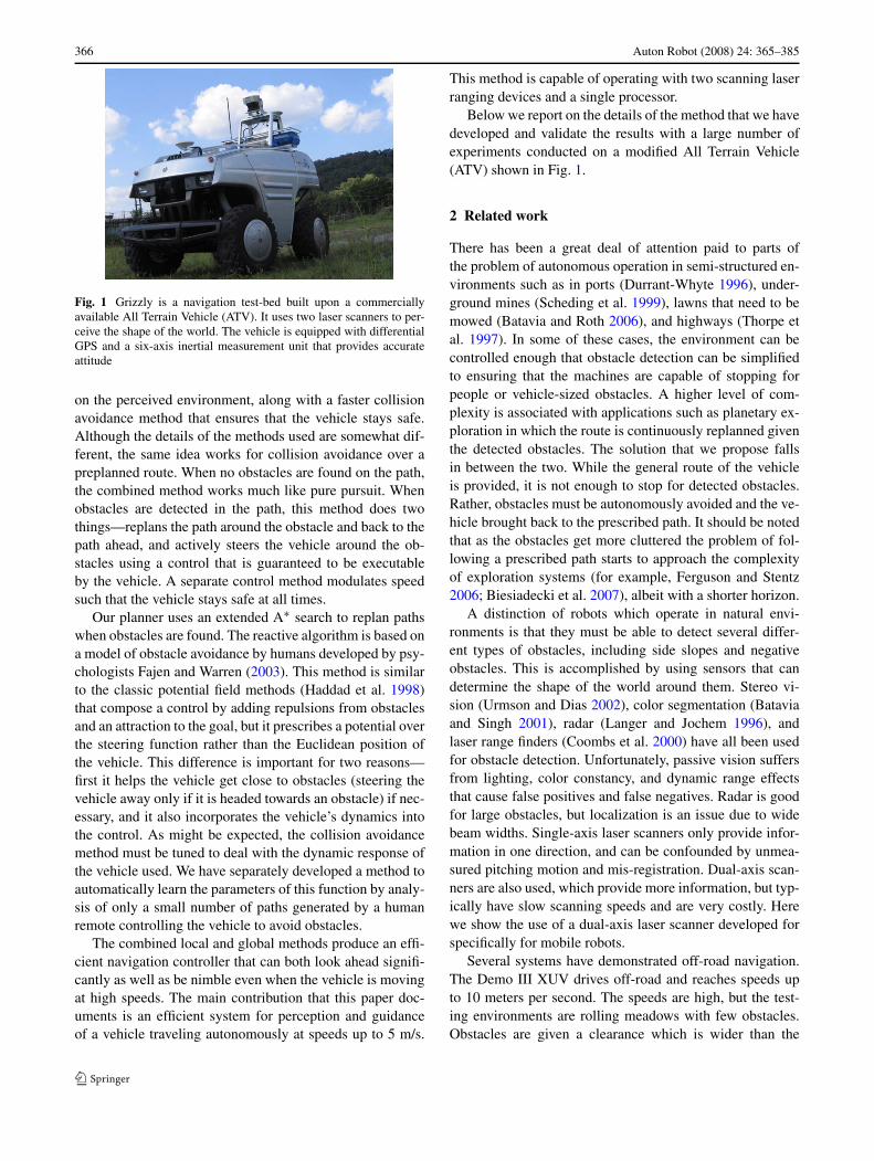
Fig. 1 Grizzly is a navigation test-bed built upon a commerciallyavailable All Terrain Vehicle (ATV). It uses two laser scanners to per-ceive the shape of the world. The vehicle is equipped with differentialGPS and a six-axis inertial measurement unit that provides accurateattitude

on the perceived environment, along with a faster collisionavoidance method that ensures that the vehicle stays safe.Although the details of the methods used are somewhat dif-ferent, the same idea works for collision avoidance over apreplanned route. When no obstacles are found on the path,the combined method works much like pure pursuit. Whenobstacles are detected in the path, this method does twothings—replans the path around the obstacle and back to thepath ahead, and actively steers the vehicle around the ob-stacles using a control that is guaranteed to be executableby the vehicle. A separate control method modulates speedsuch that the vehicle stays safe at all times.

Our planner uses an extended A∗ search to replan pathswhen obstacles are found. The reactive algorithm is based ona model of obstacle avoidance by humans developed by psy-chologists Fajen and Warren (2003). This method is similarto the classic potential field methods (Haddad et al. 1998)that compose a control by adding repulsions from obstaclesand an attraction to the goal, but it prescribes a potential overthe steering function rather than the Euclidean position ofthe vehicle. This difference is important for two reasons—first it helps the vehicle get close to obstacles (steering thevehicle away only if it is headed towards an obstacle) if nec-essary, and it also incorporates the vehicle’s dynamics intothe control. As might be expected, the collision avoidancemethod must be tuned to deal with the dynamic response ofthe vehicle used. We have separately developed a method toautomatically learn the parameters of this function by analy-sis of only a small number of paths generated by a humanremote controlling the vehicle to avoid obstacles.

The combined local and global methods produce an effi-cient navigation controller that can both look ahead signifi-cantly as well as be nimble even when the vehicle is movingat high speeds. The main contribution that this paper doc-uments is an efficient system for perception and guidanceof a vehicle traveling autonomously at speeds up to 5 m/s.

This method is capable of operating with two scanning laserranging devices and a single processor.

Below we report on the details of the method that we havedeveloped and validate the results with a large number ofexperiments conducted on a modified All Terrain Vehicle(ATV) shown in Fig. 1.

2 Related work

There has been a great deal of attention paid to parts ofthe problem of autonomous operation in semi-structured en-vironments such as in ports (Durrant-Whyte 1996), under-ground mines (Scheding et al. 1999), lawns that need to bemowed (Batavia and Roth 2006), and highways (Thorpe etal. 1997). In some of these cases, the environment can becontrolled enough that obstacle detection can be simplifiedto ensuring that the machines are capable of stopping forpeople or vehicle-sized obstacles. A higher level of com-plexity is associated with applications such as planetary ex-ploration in which the route is continuously replanned giventhe detected obstacles. The solution that we propose fallsin between the two. While the general route of the vehicleis provided, it is not enough to stop for detected obstacles.Rather, obstacles must be autonomously avoided and the ve-hicle brought back to the prescribed path. It should be notedthat as the obstacles get more cluttered the problem of fol-lowing a prescribed path starts to approach the complexityof exploration systems (for example, Ferguson and Stentz2006; Biesiadecki et al. 2007), albeit with a shorter horizon.

A distinction of robots which operate in natural envi-ronments is that they must be able to detect several differ-ent types of obstacles, including side slopes and negativeobstacles. This is accomplished by using sensors that candetermine the shape of the world around them. Stereo vi-sion (Urmson and Dias 2002), color segmentation (Bataviaand Singh 2001), radar (Langer and Jochem 1996), andlaser range finders (Coombs et al. 2000) have all been usedfor obstacle detection. Unfortunately, passive vision suffersfrom lighting, color constancy, and dynamic range effectsthat cause false positives and false negatives. Radar is goodfor large obstacles, but localization is an issue due to widebeam widths. Single-axis laser scanners only provide infor-mation in one direction, and can be confounded by unmea-sured pitching motion and mis-registration. Dual-axis scan-ners are also used, which provide more information, but typ-ically have slow scanning speeds and are very costly. Herewe show the use of a dual-axis laser scanner developed forspecifically for mobile robots.

Several systems have demonstrated off-road navigation.The Demo III XUV drives off-road and reaches speeds upto 10 meters per second. The speeds are high, but the test-ing environments are rolling meadows with few obstacles.Obstacles are given a clearance which is wider than the

Auton Robot (2008) 24: 365–385 367

clearance afforded by extreme routes. When clearance isnot available, the algorithm plans slower speeds (Coombset al. 2000). Other similar systems have been demonstratedby Kelly (1995) and Spenko et al. (2006).

In 2005, DARPA sponsored a Grand Challenge racefor autonomously driven vehicles to follow a route spec-ified by closely spaced GPS via points. This challengewas targeted exactly at the type of problem that our ap-proach intends to address. Although the race did not haveany obstacles enroute, only five out of twenty vehicles fin-ished the race (Thrun et al. 2006; Urmson et al. 2006;Trepagnier et al. 2006; Braid et al. 2006) providing a testa-ment to the difficulty of following a well-specified outdoorroute. Notably, the vehicles that did succeed were equippedwith many sensors (in some cases 8–10 laser scanners) toperceive the environment, and in most cases a large amountof computing. In contrast, our vehicle employs two laserscanners and a single processor (2 GHz Mobile Pentium).We have managed to achieve top speeds of 8 m/s (approxi-mately 28 km/h) with this system as it navigates a course atour test site.

Our work is closely related to several other research ef-forts. One connection is to a method of sensing the envi-ronment using a sweeping laser scanner (a single axis laserscanner is swiveled about an orthogonal axis) while the ve-hicle moves (Batavia and Singh 2002). This configurationallows the detection of obstacles even when the vehicle ispitching, rolling and translating.

Another connection is to the research in autonomous mo-bile robots for exploration in planetary environments (Singhet al. 2000; Urmson and Dias 2002) that uses traversabilityanalysis to find obstacles that a vehicle could encounter. Weuse a similar traversability analysis, but rather than use ele-vation maps generated from stereo vision, we use a slidingwindow of point cloud data (from multiple lasers) registeredover time to perform traversability analysis. This work hasalso typically used arc voting as a means to select betweenpaths. Subsequently, we have found that arc voting can re-sult in suboptimal paths because most or all of the arcs thatthe vehicle might consider following in the future can be in-valid, while smooth paths (e.g. S-shaped paths) through theenvironment exist.

A final connection is to a model of collision avoidanceused by humans as they navigate between discrete obstacles(Fajen and Warren 2003). Initially intended to provide anempirical model of how humans get to a point goal in thepresence of point obstacles, this method has been used byFajen et al., as a control scheme for mobile robots operatingunder some restrictions—only point obstacles are used tointerrupt a nominally straight line path to the goal while thevehicle travels at sub-meter/sec speeds (Fajen et al. 2003).Recently Huang et al., have used a modified version of themodel proposed by Fajen and Warren geared towards ob-stacle avoidance using a monocular camera (Huang et al.

2006). Since range to obstacles can not be measured directly,the width of obstacles (segmented in the image) is used in-stead of the distance. The authors report results with an in-door robot moving at 0.7 m/s. In contrast we would like ourrobot to drive outdoors at high speeds where it might en-counter various configurations of obstacles of various sizes.Furthermore, since we would like the robot to track a spe-cific path, the goal will move continuously. Below we reporton the extensions we have made to the basic model of colli-sion avoidance proposed by Fajen and Warren to allow im-plementation on an outdoor vehicle. While the researcherswho have used this methodology have found the parametersof the controller by inspection, we have developed a methodto automatically find such parameters from observation ofhuman operators. We also have developed a complementarymethod to help guide the vehicle when the environment iscluttered enough that the local avoidance scheme is insuffi-cient.

3 Obstacle detection

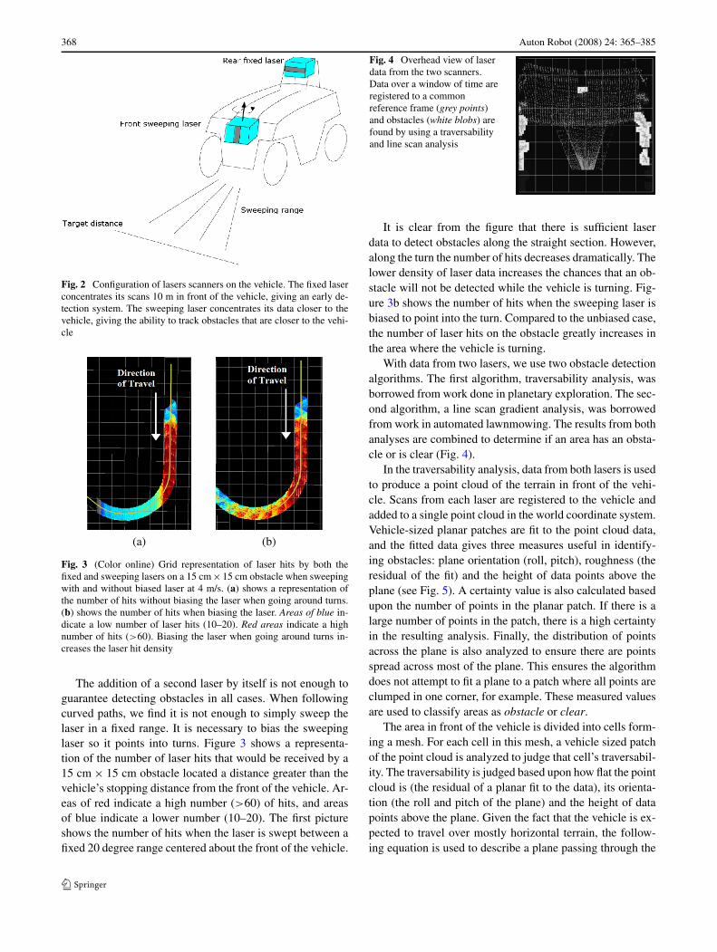
For high speed navigation, the sensors required depend onthe vehicle’s speed, stopping distance and minimum ob-stacle size. At higher speeds, where stopping distances aregreater, the obstacles must be detected at a greater distance.In order to detect smaller obstacles, the measurement den-sity of the sensor must be correspondingly greater. Our goalis to enable the vehicle to travel at speeds of up to 5 m/swhile detecting obstacles as small as 20 cm×20 cm. In otherwork with lower-speed vehicles moving at 2 m/s (Bataviaand Singh 2002), we find that a single sweeping laser is suf-ficient for detecting obstacles. The sweeping laser systemconsists of a single Sick laser turned so it is scanning a ver-tical plane. A motor mechanically sweeps the vertical planeback and forth, thus building a 3-D map of the terrain in frontof the vehicle. However, for the higher speed obstacle detec-tion in this application, we find that the sweeping laser alonecannot provide a sufficient density of laser measurements todetect small obstacles at higher speeds. Accordingly, a sec-ond fixed laser is deemed necessary (Fig. 2).

The addition of a second, fixed laser provides several ad-vantages over the single sweeping laser. Primarily, the fixedlaser is pointed 10 m in front of the vehicle and increases thedensity of laser data at points far from the front of the vehi-cle. Now smaller obstacles are detected at a distance suf-ficient for safe avoidance. The sweeping laser system con-centrates its data closer to the vehicle, so obstacles nearer thevehicle are tracked. A second advantage of the two laser sys-tem is that they collect orthogonal sets of data. The sweepinglaser is best suited for detecting pitch type obstacles, whilethe fixed laser is best suited for detecting roll type obstacles.The two laser systems complement each other by perform-ing best for these two different types of obstacles.

368 Auton Robot (2008) 24: 365–385

Fig. 2 Configuration of lasers scanners on the vehicle. The fixed laserconcentrates its scans 10 m in front of the vehicle, giving an early de-tection system. The sweeping laser concentrates its data closer to thevehicle, giving the ability to track obstacles that are closer to the vehi-cle

(a) (b)

Fig. 3 (Color online) Grid representation of laser hits by both thefixed and sweeping lasers on a 15 cm × 15 cm obstacle when sweepingwith and without biased laser at 4 m/s. (a) shows a representation ofthe number of hits without biasing the laser when going around turns.(b) shows the number of hits when biasing the laser. Areas of blue in-dicate a low number of laser hits (10–20). Red areas indicate a highnumber of hits (>60). Biasing the laser when going around turns in-creases the laser hit density

The addition of a second laser by itself is not enough toguarantee detecting obstacles in all cases. When followingcurved paths, we find it is not enough to simply sweep thelaser in a fixed range. It is necessary to bias the sweepinglaser so it points into turns. Figure 3 shows a representa-tion of the number of laser hits that would be received by a15 cm × 15 cm obstacle located a distance greater than thevehicle’s stopping distance from the front of the vehicle. Ar-eas of red indicate a high number (>60) of hits, and areasof blue indicate a lower number (10–20). The first pictureshows the number of hits when the laser is swept between afixed 20 degree range centered about the front of the vehicle.

Fig. 4 Overhead view of laserdata from the two scanners.Data over a window of time areregistered to a commonreference frame (grey points)and obstacles (white blobs) arefound by using a traversabilityand line scan analysis

It is clear from the figure that there is sufficient laserdata to detect obstacles along the straight section. However,along the turn the number of hits decreases dramatically. Thelower density of laser data increases the chances that an ob-stacle will not be detected while the vehicle is turning. Fig-ure 3b shows the number of hits when the sweeping laser isbiased to point into the turn. Compared to the unbiased case,the number of laser hits on the obstacle greatly increases inthe area where the vehicle is turning.

With data from two lasers, we use two obstacle detectionalgorithms. The first algorithm, traversability analysis, wasborrowed from work done in planetary exploration. The sec-ond algorithm, a line scan gradient analysis, was borrowedfrom work in automated lawnmowing. The results from bothanalyses are combined to determine if an area has an obsta-cle or is clear (Fig. 4).

In the traversability analysis, data from both lasers is usedto produce a point cloud of the terrain in front of the vehi-cle. Scans from each laser are registered to the vehicle andadded to a single point cloud in the world coordinate system.Vehicle-sized planar patches are fit to the point cloud data,and the fitted data gives three measures useful in identify-ing obstacles: plane orientation (roll, pitch), roughness (theresidual of the fit) and the height of data points above theplane (see Fig. 5). A certainty value is also calculated basedupon the number of points in the planar patch. If there is alarge number of points in the patch, there is a high certaintyin the resulting analysis. Finally, the distribution of pointsacross the plane is also analyzed to ensure there are pointsspread across most of the plane. This ensures the algorithmdoes not attempt to fit a plane to a patch where all points areclumped in one corner, for example. These measured valuesare used to classify areas as obstacle or clear.

The area in front of the vehicle is divided into cells form-ing a mesh. For each cell in this mesh, a vehicle sized patchof the point cloud is analyzed to judge that cell’s traversabil-ity. The traversability is judged based upon how flat the pointcloud is (the residual of a planar fit to the data), its orienta-tion (the roll and pitch of the plane) and the height of datapoints above the plane. Given the fact that the vehicle is ex-pected to travel over mostly horizontal terrain, the follow-ing equation is used to describe a plane passing through the

Auton Robot (2008) 24: 365–385 369

Fig. 5 The traversabilityanalysis fits planes to the pointcloud data to determine how flatthe area in front of the vehicleis. The roll, pitch, residual andheight of the plane are used indetecting obstacles

point cloud data:

z = Ax + By + C

In this equation x, y are the horizontal location and z is thevertical location. To find the parameters A, B , and C, linearregression (Press et al. 1992) is used to fit all N points byminimizing the residual.

r =N∑

i=1

(zi − Axi + Byi + C)2/N

The residual of the plane fit gives a measure of how roughis the terrain. However, terrain roughness is not the only ob-stacle type of interest. Terrain that is significantly sloped canbe a roll-over hazard. For this reason, we also measure theorientation of the plane. Given the A, B , C parameterizationof the plane we can determine the vehicle’s roll and pitch ifit was resting on the plane at a given yaw angle

pitch = arcsin

(B cos(yaw) − A sin(yaw)√

A2 + B2 + 1

)

roll = atan(−A cos(yaw) − B sin(yaw))

In this application, the point cloud is generated in a vehicle-centered frame, and to simplify the plane orientation analy-sis we assume the vehicle will maintain its current head-ing (yaw = 0). This decreases the execution time of the tra-versability analysis.

The above analysis is performed on the entire vehicle-sized patch of the point cloud data. However, it can misssmall obstacles which may be lying in the vehicle’s path.These types of obstacle may have a relatively small effecton the residual of the plane fit and so would not be found ifonly the residual is used to detect obstacles. For this reason,each vehicle size planar patch is itself broken into smallercells that are individually analyzed to find the patch residualand step height (see Fig. 5). For these analyses, the points inthe vehicle-sized patch outside of the cell are fit to a plane,and the residual is calculated of the points inside the cellwith respect to this plane. The patch residual is the maxi-mum value of this residual for all cells in the vehicle sized

patch. For each cell, the variance in the point heights is alsoanalyzed. The step height for the vehicle-sized patch is cal-culated as the maximum variance in the cells’ point heights.

These five values, residual, roll, pitch, patch residual, andstep height, are used to measure the traversability. Each ofthese values is given a hazard score between 0 and 1. A valueof 0 indicates an obstacle, and a value of 1 indicates a cleararea

hazardScore(value,goodValue,badValue)

=

⎧⎪⎨

⎪⎩

1 if value < goodValue

0 if value > badValuemax−valmax−min otherwise

The overall traversability of a cell is given the minimumof the 5 hazard scores. The good and bad ranges of eachof these obstacle detection parameters needs to be tuned insuch a way that true obstacles are detected while a minimumof false obstacles are detected. The obstacles also need tobe detected at a range at which they can be avoided easily.The number of parameters and the difficulty of the detec-tion problem made hand-tuning of these parameters difficult.A more reasoned approach was necessary.

To choose the good and bad values used in the hazardscores, we needed to measure and compare the residual, roll,pitch, etc. parameters in areas of obstacles and clear areas.To do this, the vehicle was driven at high speed throughan open field with a set of surveyed obstacles sized 50 cm,30 cm and 20 cm (see Fig. 6). Because the obstacles are sur-veyed, the areas where obstacles and clear areas should bedetected are known, and the obstacle detection parameterscan be measured and compared in the two areas. Figure 7shows histograms of the residual as measured in clear andobstacle areas. As is expected, in areas without obstacles,the residual measured is relatively low. In areas of obstacle,the residual is much higher. Also of note is that the two dis-tributions are well separated. Figure 7 also shows a plot ofthe confidence that a given residual value corresponds to ei-ther an obstacle or clear area. This confidence measure istaken from the same data shown in the histograms, and isthe percentage of values measured that are less than a given

370 Auton Robot (2008) 24: 365–385

residual value. The good and bad values for the residual arechosen to minimize the likelihood of false obstacle detectionwhile simultaneously attempting to maximize the likelihoodof true obstacle detection. In this case, a good (clear) resid-ual value was chosen to be 0.003 m2. 99.5% of the measured

Fig. 6 This figure shows the path driven and obstacle locations usedto determine the hazard parameters. To measure the hazard parametersused in detecting obstacles, the vehicle was manually driven at approx-imately 4 m/s through an open field with surveyed obstacles. Becausethe obstacle locations are known, the hazard parameters can be mea-sured and compared in areas known to be clear or occupied by an ob-stacle. The path used for measuring the hazard parameters is shown inblack. The surveyed obstacles are shown as the three stars

residuals in the clear areas are less than this value and lessthan 15.2% of the measured residuals in the obstacle areasare less than this value. That is, at this residual value thereis a very high probability that it represents a clear area anda small probability of being an obstacle. The bad (obstacle)residual value was chosen to be 0.005 m2. 0.3% of the clearresidual values are greater than this value and 70% of theobstacle residual values are greater than this value. That is,at this value there is an extremely low probability the area isclear, but a very high probability that it is an obstacle. Theremaining hazard values were chosen in a similar way.

While the traversability analysis is a simple way of de-tecting obstacles, it can produce false positives due to inac-curate calibration of the two lasers and/or incorrect synchro-nization with positioning. To supplement the traversabilityanalysis, the slope of segments of individual line scans fromthe sweeping laser is also calculated as in Batavia and Singh(2002). If the slope of a scan segment is above a giventhreshold, it is tagged as a gradient obstacle (Fig. 8). Be-cause the gradient analysis uses piecewise segments of anindividual line scan, it is not susceptible to mis-registrationas the traversability analysis can be.

To classify an object as a true obstacle, both the gradientand traversability analyses must agree. The combination ofthe two obstacle detection algorithms compensates for theweaknesses of the two individual algorithms and dramati-cally reduces the false obstacle detection rate. Because thegradient analysis looks at only an individual line scan fromthe sweeping laser, it cannot take advantage of integratingmultiple scans over time like the traversability analysis can.However, by only using single line scans, the gradient analy-sis is relatively immune to mis-registration problems thatplague the traversability analysis.

Fig. 7 The left plots show histograms of the residual measured in clear and obstacle areas. The right plot shows the confidence that a givenresidual value is either obstacle (.) or clear (+) area

Auton Robot (2008) 24: 365–385 371

Fig. 8 The line scan analysis uses an individual line scan from thesweeping laser. The slope local to a scan point is used to determine ifthat point represents an obstacle or clear area

3.1 Precisely locating the laser scanners

Because the traversability analysis integrates multiple laserscans over a period of time to detect obstacles, the lasersmust be calibrated (that is, located precisely in the vehi-cle reference frame) to avoid false positives and negativesin obstacle detection. The laser scanners can be calibratedby finding a 6 DOF transformation that locates each in thereference frame of the robot. For any point in the sweepinglaser coordinate frame Lp̂ , a transformation matrix from thelaser coordinate frame to the robot coordinate frame R

LM isgiven by

RLM = R

LT RLR (1)

Translation and rotation matrices are denoted by

RLT =

⎡

⎢⎢⎣

1 0 0 xs

0 1 0 ys

0 0 1 zs

0 0 0 1

⎤

⎥⎥⎦ (2)

RLR =

⎡

⎢⎢⎣

1 0 0 00 cos θs − sin θs 00 sin θs cos θs 00 0 0 1

⎤

⎥⎥⎦

×

⎡

⎢⎢⎣

cosφs 0 sinφs 00 1 0 0

− sinφs 0 cosφs 00 0 0 1

⎤

⎥⎥⎦

×

⎡

⎢⎢⎣

cosψs − sinψs 0 0sinψs cosψs 0 0

0 0 1 00 0 0 1

⎤

⎥⎥⎦ (3)

where xs , ys , and zs are translations and θs , φs , and ψs arethe angles for roll, pitch, and yaw. Similarly, a transforma-tion matrix from the fixed laser coordinate frame to the robotcoordinate is given by

RL′M = R

L′T RL′R (4)

We calibrate the system by collecting laser data from thevehicle sitting stationary and pointing at two targets, a verti-cal plane and a horizontal plane. These targets are registeredwith a portable differential positioning system (DGPS) for

establishing ground truth. Then the calibration parametersare found by minimizing the distance of the measured pointsfrom their corresponding ground truth data.

We compute the transformation matrix from the worldcoordinate to the robot coordinate using the position and ori-entation of the vehicle. We obtain that data from the DGPSof the vehicle. Then we transform the ground truth datafrom the world coordinate frame to the vehicle’s coordinateframe. We use singular value decomposition (SVD) to ob-tain the plane parameters, a, b, c and d . The vertical planeis given by

aviRxvi + bvi

Ryvi + cviRzvi + dvi = 0 (5)

The horizontal plane is given by

ahiRxhi + bhi

Ryhi + chiRzhi + dhi = 0 (6)

where i = 1,2,3, . . . , n (n is the number of vehicle posi-tions where we survey the targets using two laser sensors).(Rx,R y,R z) is a point on the vertical or the horizontal planein the vehicle’s coordinate frame.

After that, we optimize xs , ys , zs , θs , φs and ψs whichminimize Eh and Ev . Eh and Ev are the distance from themeasured points to the corresponding plane. This optimiza-tion is a non-linear least squares problem. Necessary equa-tions for this optimization are as follows,

RLM = R

LT RL R (7)

[Rx,Ry,Rz]T = RLMLp̂ (8)

where Lp̂ = [Lx,Ly,Lz]T

Eh = ahiRxhi + bhi

Ryhi + chiRzhi + dhi√

a2hi + b2

hi + c2hi

(9)

Ev = aviRxvi + bvi

Ryvi + cviRzvi + dvi√

a2vi + b2

vi + c2vi

(10)

min1

2‖E(p)‖2 = 1

2

∑(Evi

2 + Ehi2) (11)

where i = 1,2,3, . . . , n.Next,we want to obtain the fixed laser parameters xf ,

yf , zf , θf , φf and ψf . At this time, we use the result ofthe sweep laser calibration instead of using the ground truthplane. First, we transform the sweep laser sensor data fromthe sweep laser coordinate to the robot coordinate.

Rp̂vi = RLMi

Lp̂vi (12)

After that we use SVD

Rp̂vi[avi, bvi, cvi, dvi]T = 0 (13)

SVD(Rp̂vi) = UviSviVTvi (14)

372 Auton Robot (2008) 24: 365–385

The eigenvector corresponding to the smallest eigenvaluecontains the vertical plane parameters avi , bvi , cvi and dvi .Similarly, using

SVD(Rp̂hi) = UhiShiVThi (15)

we get the horizontal plane parameters, ahi , bhi , chi and dhi .We optimize the fixed laser parameters using these new pa-rameters. The method for this optimization is the same asthat of the sweep laser calibration. Now, we have the cali-bration parameters of the sweep and fixed laser sensors. Formore details about the data collection and the fitting proce-dure, please see Takahashi et al. (2007).

4 Dodger: local collision avoidance

The goal of our collision avoidance system is to follow apath and avoid obstacles along the way. When an obstacleis detected in front of the vehicle, the vehicle should swerveto avoid it and return to the path in a reasonable fashion.If there are multiple obstacles on the path, the vehicle mustnavigate between them. Sometimes an obstacle may blockthe entire path. In this case, the vehicle must stop before col-liding with it. An ideal collision avoidance algorithm wouldaccept a map of hazards and determine steering and speedto navigate in between these. Since this algorithm must runmany times a second, ideally it would have low computa-tional complexity.

4.1 Formulation

Fajen and Warren’s model uses a single goal point whichattracts the vehicle’s heading. This attraction increases asthe distance to the goal decreases and as the angle to thegoal increases, yielding the goal attraction function

attractFW(g) = kg(φ − ψg)(e−c1dg + c2)

We represent the vehicle’s heading with φ. (φ − ψg) is theangle to the goal. dg is the distance to the goal. kg , c1, andc2 are parameters which must be tuned.

Similarly, each obstacle repulses the agent’s heading. Therepulsion increases with decreasing angle and decreasingdistance. Then for each obstacle, there is a repulsion func-tion:

repulseFW(o) = ko(φ − ψo)(e−c3do)(e−c4|φ−ψo|)

(φ −ψo) is the angle to the obstacle. do is the distance to theobstacle. ko, c3, and c4 are parameters which must be tuned.

The goal attractions and obstacles repulsions are summedtogether, applying superposition, and damped with the cur-rent heading rate and a damping factor b to get a headingacceleration command. The result is a single control law:

φ̈∗FW = −bφ̇ − attractFW(g) +

∑

o∈O

repulseFW(o)

Note that superposition will not always yield good re-sults. There are many situations in which attractions and re-pulsions can oppose each other in such a way as to cause thevehicle to avoid obstacles improperly. This is a limitation ofthe system. It is up to the user to find good parameter valuesto prevent these situations from occurring as much as pos-sible. Also, in the next section, we will present our methodfor dealing with these cases when they are unavoidable.

Fajen and Warren’s proposed algorithm is ideal in that itscommands are guaranteed to be achievable by the vehicle,producing smooth paths. It is also computationally efficient,with a run time linear in the number of obstacles. However,this algorithm does make certain assumptions regarding thegoal being a fixed point and the size and placement of obsta-cles. Next we present a series of modifications which allowus to apply this algorithm to a vehicle tracking a path withlarge obstacles which may be densely packed. We call the re-sulting path-tracking obstacle avoidance system DODGER.

In our situation, a desired path is given. We set the goalpoint to be a large distance along the path from the vehicle’scurrent location. Since the goal is always nearly the samedistance from the vehicle, we do not need a distance term inour control law (called MFW for modified Fajen/Warren):

attractMFW(g) = kg(φ − ψg)

Also, we found that FW works well for individual point ob-stacles, but in dense obstacle configurations more informa-tion is needed. In preliminary tests, we frequently observedthe vehicle oversteering on curves due to repulsion from ob-stacles which were directly in front of the vehicle but farfrom its intended path. In these situations, the attraction ofthe goal is enough to assure the vehicle will avoid the obsta-cles. Using FW, though, the extra repulsion could even causethe vehicle to steer towards a small obstacle on its intendedpath. The obstacle on the path should have more weight thanthose off the path. Rather than decrease the weight of anyobstacles, we add a term to the repulsion equation to putadditional weight on obstacles between the vehicle and thegoal:

repulseMFW(o) = ko(φ − ψo)(e−c3do)(e−c4|φ−ψo|)

× (1 + c5(dmax − min(dmax, dgv)2))

For the last term, we draw a vector from the vehicle to thegoal point. An obstacle’s repulsion is increased in proportionto its distance, dgv , to that vector. If the distance is greaterthan dmax, then no extra weight is applied. This maximumdistance is based on the maximum distance the vehicle isallowed to be off the path. We use the goal vector term as anapproximation of the obstacle’s distance to the desired path,as it is simpler and quicker to calculate than the distanceto the path. The approximation loses effectiveness when the

Auton Robot (2008) 24: 365–385 373

Fig. 9 Distance and angleterms used in the MFW controllaw. We consider the vehicle’sposition to be the center of therear axle, so all distances aremeasured from that point

path curves very sharply. However, in practical situations,we have found these cases to be rare.

With these modifications we are left with the controlequations which make up the Dodger algorithm:

φ̈∗MFW = −bφ̇ − kg(φ − ψg)

+∑

o∈O

ko(φ − ψo)(e−c3do)(e−c4|φ−ψo|)

× (1 + c5(dmax − min(dmax, dgv)2))

φ̇∗MFW = φ̇ + (�t)φ̈∗

MFW)

The attraction of the goal and obstacle repulsion are summedtogether and damped with the heading rate φ̇ with the damp-ing factor b to get a commanded heading acceleration φ̈∗.The low-level controller for our vehicle accepts heading ratecommands, so the heading acceleration is then integrated us-ing the iteration time �t and then added to the current head-ing rate. See Fig. 9 for an illustration of the terms used inthe MFW control law.

4.2 Implementation on a vehicle

The success of the Dodger algorithm is contingent on valuesof the parameters which control the attraction of the goal andrepulsion of the obstacles. We have developed an automatedlearning system to determine the best values for these para-meters. The system begins with the collection of data froma human operator steering the vehicle to follow a path andavoid obstacles. The operator sits on the vehicle and driveswhile looking at a display of the desired path and the obsta-cles supplied from our obstacle detection system. In this waythe operator receives feedback of how far away he is fromthe desired path and at what time the obstacles are detected(so he knows at what time to start turning).

We manually segmented the driving data into short seg-ments in which the operator avoided one or more obstaclesand returned to the path. Including data without obstaclescould have negatively affected the learning results, since thisdata would not constrain the obstacle repulsion parameters,only the goal attraction parameters.

With only a few training data segments, covering approx-imately 30 meters of driving, we ran a number of machinelearning algorithms. These included gradient descent, sim-ulated annealing, a genetic algorithm, and simple randomguesses. The error values for potential parameter sets werecalculated by producing a simulated path of how the au-tonomous control system would drive using the parameterset in the same scenario as the training segment. Error wasdefined as the point-wise distance from the simulated pathto the training path, plus a penalty for steering oscillation.We found that in general the randomized techniques (ge-netic algorithms and random guessing) produced parametersets with lower error. The lowest error parameter set wasproduced from the random guess method. We tested this pa-rameter set against a hand-tuned parameter set which we hadbeen using previously to the learning work. In an extendedseries of tests running the system with each parameter setthrough identical obstacle scenarios, the learned parameterset significantly outperformed the hand-tuned set. We usedthe learned parameter set for later obstacle avoidance exper-iments and vehicle endurance tests. For more information,please see Hamner et al. (2006).

In Fajen and Warren’s model each obstacle was a sin-gle point. However, as discussed in the previous section, ourobstacles can be of arbitrary size and shape. Obstacles arecommunicated from the obstacle detection system as an un-ordered series of points. We needed to store the obstacle datain a way that allows the system to efficiently iterate throughevery known obstacle while also allowing for easy additionand deletion and a lookup procedure to determine if there isan obstacle in a given location. A map representation is bestfor addition and deletion of obstacles, but it must be largeenough to cover the complete area of driving. Also, therewill be many empty cells, which will slow down the com-putation of the obstacle repulsion because the system mustsearch through every cell for detected obstacles. A linkedlist or an array would lend to easy computation of the re-pulsion, but addition and deletion would be slow. We imple-mented a hash table to store the obstacles, with the x- andy-coordinates as the key to the hash function. Deletion isrelatively quick, because the system does not have to searchthrough every obstacle to find the desired one. The compu-tation of the repulsion is also quick, because there are rela-tively few empty bins, and the hash table does not explicitlyrepresent all possible obstacle locations.

After receiving a list of points from the obstacle detec-tion system, the collision avoidance system then discretizesthe points onto a ten centimeter grid (see Fig. 10) and storesthem in the hash table buffer. If all obstacle points were fedto Dodger, then large obstacles would have an unjustifiablyhigher weight than small obstacles. To remove this bias, forevery obstacle point, the system determines whether it is onthe leading edge of an obstacle relative to the vehicle by

374 Auton Robot (2008) 24: 365–385

Fig. 10 Illustration of how our system discretizes obstacles and usesthem in Dodger. The obstacle detection system finds the obstacles andsends the points to the collision avoidance system, which discretizesthem in small cells (grey points). Then when calculating the obstaclerepulsion in Dodger, only the leading edge points (black) are used.(Vehicle not drawn to scale with the grid)

searching the next two cells in the direction of the vehicle.If there is no obstacle point in those cells, the reference pointis on the leading edge of an obstacle. Obstacle repulsion isonly calculated for those points on the leading edges of ob-stacles.

Fajen and Warren found that most subjects walked at aconstant pace, so they did not explore speed control. Weconstructed a speed control function based on the obstacle’sdistance and angle:

v = mino∈O

[do

2 cos(|φ − ψo|)]

This slows down the vehicle as obstacles get closer, whichallows sharper turning and more time for the system to de-tect additional nearby obstacles. In addition, the system pre-dicts the vehicle’s course using the MFW control law for thenext few seconds. If the vehicle is forced to stop for an ob-stacle in the next few seconds, the system slows it down im-mediately. For quick computation, this is only a kinematicsimulation. It assumes all steering commands are instantlyachieved with the vehicle traveling in perfect arcs for half-second intervals.

Finally, there are some cases in which Dodger would ex-hibit undesirable behavior while not actually colliding withan obstacle. For example, Fig. 11 shows a case where an ob-stacle can push the vehicle off its desired path, even thoughthe path is clear. To prevent the vehicle from unnecessarilydiverging from the desired path, we use a “ribbon” method.We construct a ribbon of fixed distances down the path andto either side. If there are no obstacles on this ribbon and thevehicle is currently within the ribbon, then we zero any ob-stacle repulsion. The result is a steering angle entirely basedon the goal attraction, and the vehicle successfully tracks thepath.

Fig. 11 Illustration of the need for the ribbon surrounding the path.The vehicle attempts to go towards the goal on the right, but the obsta-cle off the path unnecessarily repels the vehicle leftward

4.3 Analysis of damping

When operating a vehicle at high speeds, the issue of re-sponsiveness versus smoothness in the control becomes animportant one. The vehicle needs to be able to turn quicklyenough to avoid obstacles, but oscillations in the steeringcommand could shake or, in the worst case, flip the vehicle.Achieving a balance between these two is required whenmaking a good controller. To explore the role of dampingin the system we conducted a number of experiments, eachhighlighting a different aspect of the problem.

Recall the Dodger control law equations with the damp-ing term:

φ̈∗ = −bφ̇ − attractMFW(g) +∑

o∈O

repulseMFW(o)

φ̇∗ = φ̇ + �tφ̈∗

Our first question was whether to damp on the measuredheading rate or the heading rate command from the previouscontrol iteration. We would expect damping on the measuredheading rate to be more stable, in that then the system wouldbe responding to what is actually happening to the vehicle.However, we discovered that the heading rate measurementfrom our INS/GPS system (see Fig. 12) is particularly noisy,varying by plus or minus three or more degrees per secondbetween every iteration. Damping on this measurement in-troduced that noise into the control system and caused thecontrol to become less stable (Fig. 13).

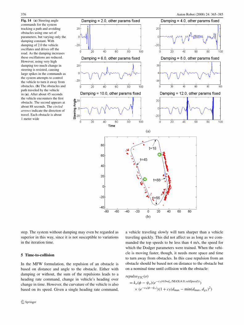
With the damping model based on the commanded head-ing rate, we then wanted to explore how the level of dampingwould affect the system control. First we used our learningprocess for the model and derived a parameter set with adamping factor of 6.0. Then we ran a series of experiments,running the vehicle over the same stretch of road with obsta-cles, and each time varying only the damping factor. We ranthe vehicle six times, with the damping factor varying be-tween 2.0 and 12.0. The results are in Fig. 14. As expected,the vehicle oscillates too much with damping factors of 2.0and 4.0. The response is good with damping of 6.0 and 8.0.

Auton Robot (2008) 24: 365–385 375

Fig. 12 Measurements from the localization system. The vehicle, ata stop, is commanded to go 4 m/s with zero curvature. As the vehi-cle moves, the heading rate reading varies by a few degrees betweenevery reading, despite the vehicle moving mostly straight. If we dampthe Dodger system using the measured heading rate, this noise is intro-duced into the command

With 10.0 and 12.0 we start to see too much resistance toturning the vehicle. To start turning the vehicle, the controlsystem has to overcome whatever damping is applied. Thedamping acts as a delay. As the vehicle passes an obstacle,there is a “sweet spot” for its heading, at which the goal at-traction and obstacle repulsion balance each other and createstability. With large damping, there is a large delay, and thevehicle oscillates about the heading that the control systemis trying to achieve. Figure 15 shows a breakdown of thecommands into goal, obstacle, and damping contributions.Note the positive feedback in the damping term when thedamping factor is 12.

Finally, we questioned whether damping is really neces-sary in the control system. There is a natural damping in thevehicle itself due to the dynamics of the steering actuator,which has its own delay and dead-band. We characterizedthe dynamics of the actuator by sending a series of steeringangle commands to the vehicle and recording measurementsfrom an encoder attached to the steering column. We wereable to derive a second order relationship from this data:

θ̈ = −bθ̇ − k(θ − θd)

b = 6.836

k = 25.929

tdelay = 0.25 s

To remove the damping we constructed a new control equa-tion in which the attraction from the goal and repulsion fromobstacles are treated as direct influences on the heading rateof the vehicle, rather than heading accelerations:

φ̇∗ = −attractMFW(g) +∑

o∈O

repulseMFW(o)

(a)

(b)

Fig. 13 (a) Path driven by the vehicle when damping on the mea-sured heading rate (solid line) and the commanded heading rate (dot-ted line). The circled arrow indicates the vehicle’s direction of travel.(b) The commanded heading rates for each system over the period oftime shown in (a). The measured-damping model has higher oscilla-tions due to noise in the heading rate measurement

We ran the learning process using this model to get a newsystem with its own parameters. Then we tested this controlsystem and the system with damping 6.0 in a number of sce-narios. They each had the same record regarding obstacles;neither got stuck in the scenarios we tested on. This is asexpected, since the learning process trained both systems todrive in the same way around obstacles. However, as shownin Fig. 16, we found little difference in the amount of oscil-lation in the heading rate commands. This was a surprisingresult. Note the learning process also penalizes oscillation.It may be possible that in order to get the correct responseto obstacles that some minor oscillation is necessary, or thatthe penalty for oscillation works well enough that it alreadyproduces the smoothness normally associated with damping.

The results of the experiments indicate that the perfor-mance of the two systems is close enough to be consideredequal in quality. There is not much difference in the calcula-tion cost; the system with damping requires one integration

376 Auton Robot (2008) 24: 365–385

Fig. 14 (a) Steering anglecommands for the systemtracking a path and avoidingobstacles using one set ofparameters, but varying only thedamping constant. Withdamping of 2.0 the vehicleoscillates and drives off theroad. As the damping increasesthese oscillations are reduced.However, using very highdamping too much change insteering is resisted, causinglarge spikes in the commands asthe system attempts to controlthe vehicle to turn it away fromobstacles. (b) The obstacles andpath traveled by the vehiclein (a). After about 45 secondsthe vehicle encounters the firstobstacle. The second appears atabout 88 seconds. The circledarrows indicate the direction oftravel. Each obstacle is about1 meter wide

(a)

(b)

step. The system without damping may even be regarded assuperior in this way, since it is not susceptible to variationsin the iteration time.

5 Time-to-collision

In the MFW formulation, the repulsion of an obstacle isbased on distance and angle to the obstacle. Either withdamping or without, the sum of the repulsions leads to aheading rate command, change in vehicle’s heading overchange in time. However, the curvature of the vehicle is alsobased on its speed. Given a single heading rate command,

a vehicle traveling slowly will turn sharper than a vehicletraveling quickly. This did not affect us as long as we com-manded the top speeds to be less than 4 m/s, the speed forwhich the Dodger parameters were trained. When the vehi-cle is moving faster, though, it needs more space and timeto turn away from obstacles. In this case repulsion from anobstacle should be based not on distance to the obstacle buton a nominal time until collision with the obstacle:

repulseTTC(o)

= ko(φ − ψo)(e−c3(4.0∗do/MAX(4.0,vehSpeed)))

× (e−c4|φ−ψo|)(1 + c5(dmax − min(dmax, dgv)2)

Auton Robot (2008) 24: 365–385 377

(a) (b)

(c) (d)

Fig. 15 Breakdown of the command for three different damping mod-els over time as the system drives the vehicle down a path with obsta-cles. In (a) the undamped heading rate model introduced at the end ofSect. 4.3, (b) the heading rate model with a damping value of 6, and(c) the heading rate model with a damping value of 12. In each, thetop profile is the goal attraction contribution, second is the obstacle re-pulsion contribution, third is the contribution of damping, and fourth isthe heading rate command resulting from the sum of those three. The

no damping model and the damping 6 model perform similarly. Withdamping 12, the motion is resisted too much, causing the system tosend increasingly sharper commands, a positive feedback in the damp-ing contribution, and the vehicle to oscillate. (d) The test path labeledwith the approximate times at which an obstacle is reached. The circledarrows indicate the direction of travel. Obstacle widths range from 1 to2 meters

378 Auton Robot (2008) 24: 365–385

Fig. 16 (Color online) (a) Pathdriven by the vehicle whenusing the damping formulationand the non-dampedformulation. The marked pointsare indices of the nominal pathfor reference in (b) and (c). Thecircled arrows indicate thedirection of travel. Eachobstacle is about 1 meter wide.(b) With the system usingdamping, the steering anglerelative to the path index of thevehicle; that is, the index of theclosest point on the nominalpath to the vehicle. In blue, thesteering angle command fromDodger. In red, the effectivesteering angle measured fromthe INS/GPS system.(c) Steering angle with thesystem using the non-dampedformulation. The two systemshave a similar steering responseover most of the path, especiallyduring goal-tracking situations.Small differences were observedin obstacle avoidance situations,as the non-damped system had aslightly quicker response andalso required less sharp steering

(a)

(b)

(c)

To get the nominal time to collision we divide the dis-tance to the obstacle by the current vehicle speed, cappedby a minimum of 4.0 m/s. Then we normalize by multi-plying it by 4.0, the speed for which the parameters weretrained. This ensures that operation continues normally atslow speeds.

We ran the system with the original formulation (nodamping) and with the time-to-collision formulation fivetimes each, with maximum speeds varying from 4 to 8 m/s.The test path was a straightaway, allowing the vehicle to

get up to top speed, with a single obstacle. The results areshown in Fig. 17. With the original formulation, the vehi-cle starts turning at the same point on the path regardlessof speed. At the higher speeds the vehicle got closer tothe obstacle. The system did not command it to turn sharpenough initially, it continued to drive towards the obsta-cle, and then a very high turn command was required tokeep the vehicle from colliding or getting stuck. With thetime-to-collision mode, the vehicle started turning meterssooner.

Auton Robot (2008) 24: 365–385 379

(a) (b)

(c)

Fig. 17 Comparison of the normal Dodger model, where obstacleweight is based on distance and angle, with the time-to-collisionmodel. For the comparison we set up a path with an obstacle at 172meters down the path. With each model, the system was run down thepath five times, with maximum speeds 4, 5, 6, 7, and 8 m/s. Each plotshows the heading rate command to the vehicle as a function of dis-tance traveled down the path. In (a), with the normal model, the systemstarts commanding the vehicle to turn at approximately 169 meters re-gardless of the commanded speed. In (b), with the time-to-collision

model, the system starts commanding the vehicle to turn sooner athigher speeds. At 8 m/s (bottom plot), the turn starts at 166 metersdown the path. (c) The path taken by the vehicle with the system usingthe normal Dodger model (solid line) and the time-to-collision model(dotted line), both with a maximum speed of 7 m/s. The circled arrowindicates the direction of travel. The vehicle starts turning over twometers sooner using the time-to-collision model. The obstacle is over1 meter wide

6 Dodger with planning

There are situations in which Dodger does not find a patharound the obstacle, and the vehicle is forced to stop. Whenthe obstacle is wide, there are points on both sides of thevehicle which counteract each other, so the vehicle nevergets all the way around the obstacle (Fig. 18a). Also, whenthere is an obstacle around a corner, Dodger prefers to gooutside the turn around the obstacle, rather than inside. Thisis because the obstacle points on the inside of the turn arecloser to the goal vector, and therefore have more repulsion.This causes a problem when the obstacle covers the outsideof the corner (Fig. 18b).

Using the predicted path, the system can detect situationsin which Dodger fails to direct the vehicle around the obsta-

cle. When the predicted path stops in front of an obstacle,the system invokes a planning algorithm, like A∗, to get anew goal point which will help Dodger around the obsta-cles. First, the planning algorithm constructs a small map ofthe area in the vicinity of the vehicle (Fig. 19a). The goallocation passed to A∗ is Dodger’s goal point. Next, the plan-ning algorithm finds the optimal path around the obstaclesto that goal location. The system then starts at the goal pointand walks backwards along the optimal path, stopping whenthere are no obstacles on a straight line to the vehicle. Thisunblocked position is selected as a new goal for Dodger,and the Dodger algorithm is run again. The new goal pointis closer than the old one, and is off to one side of the prob-lem obstacles, so it has more influence than the original goal

380 Auton Robot (2008) 24: 365–385

(a) (b)

Fig. 18 In (a), due to the curved shape and width of the obstacle,some of the rightward repulsion is cancelled out by a leftward repul-sion. Then Dodger does not find a way all the way around the obstacle,and stops before a collision. In (b), there is enough room to avoid this

obstacle to the left. However, the obstacle points closer to the goal vec-tor exhibit a larger rightward repulsion. The obstacle is too wide forthe vehicle to avoid around the outside, so Dodger stops the vehiclebefore collision

(a) (b) (c)

Fig. 19 In (a), the system predicts a stuck situation and invokes A∗.The map covers only a small area between the vehicle and the originalgoal point. Obstacles are added to the map, and points within the ve-hicle’s minimum turning radius are also marked as untraversable. Theoptimal path from A∗ goes around the obstacle, and the furthest visiblepoint along the A∗ path is set as the new goal point. Dodger is run again

using this goal. In (b), the new A∗ goal point has pulled the vehicle alittle to the left, but not far enough yet, since the system still predictscollision. A∗ continues to be invoked. In (c), the vehicle is far enoughto the left that the system no longer predicts a collision if the regulargoal point is used with Dodger, so A∗ is no longer necessary

(a) (b) (c)

Fig. 20 The A∗ augmentation to Dodger can also lead the vehiclethrough complex configurations of obstacles. In (a), Dodger finds noway around the wall of obstacles, so A∗ is invoked. In (b), the goal

obtained from the D∗ path pulls the vehicle to the left. In (c), Dodgeralone can navigate the vehicle past the remaining obstacles

Auton Robot (2008) 24: 365–385 381

Fig. 21 Diagram of the entire system. Data from the laser scannersand the laser encoders goes to a controller board over serial. Data fromthe laser controller board and the INS/GPS system go to the main com-

puter over ethernet. Information is shared between the processes on themain board via shared memory. Steering and velocity commands aresent to the vehicle controller board via ethernet

382 Auton Robot (2008) 24: 365–385

Fig. 22 In a series of extendedtests we ran the system with amaximum speed of 5 m/s on alooping path on our test vehicleuntil the vehicle’s batteries werecompletely discharged. Obstaclewidths ranged from 1 meter to3 meters. (a) Here is a plot ofthe vehicle’s path over one suchtest. The vehicle ran over 22 kmand did not get stuck, a total of72 loop iterations. The blackline shows the nominal pathgiven to the system.(b) A close-up the mostcomplex obstacle scenario in theloop from (a), to emphasize therepeatability of the system. Thearrows indicate the vehicle’sdirection of travel

(a)

(b)

point. When Dodger is run again, the new goal point pullsthe vehicle to one side of the obstacles. In essence, the plan-ning algorithm chooses a side for Dodger to avoid on. Thesystem continues this hybrid method until Dodger, using itsnormal goal point, gives a predicted path that safely avoidsthe obstacles (Fig. 19c). The A∗ augmentation to Dodgeris especially useful in complex obstacle configurations, asshown in Fig. 20. Running Dodger with the planning algo-rithm takes more computation time, so to be safe, we alsoslow the vehicle down when the planning algorithm is run-ning.

7 Results

The system presented here (Fig. 21) is able to perform highspeed off road navigation at speeds up to 5m/s. The tightlycoupled GPS + IMU localization system provides reliableposition estimates in areas with limited GPS availability.The combination of two laser systems, one fixed and theother sweeping, enables us to detect obstacles as small as30 cm high and 30 cm wide. The obstacle avoidance algo-rithm allows us to avoid these obstacles even while travelingat 5m/s.

Auton Robot (2008) 24: 365–385 383

(a)

(b)

(c)

Fig. 23 Example of recovery from stuck states with one 3-meter-wideobstacle and a 5-meter-wide obstacle. The circled arrow indicates thedirection of travel. In this situation, the vehicle approached the obsta-cles from below, failed to turn soon enough, and came to a stop in frontof the leading obstacle (a). The user manually backed up the vehicle afew meters (dotted line) and restarted the system (b). The system wasthen able to steer the vehicle around the obstacles (c)

To show the robustness of the system we performed a se-ries of tests on a looping road. We placed a series of obstaclescenarios along the path, one or more obstacles in a scenario,with obstacle widths ranging from 1 to 5 meters. In each testwe set the system to autonomously repeat the loop and let itrun until the vehicle’s batteries had been nearly discharged,which was typically after about 20 km of driving. One suchtest is shown in Fig. 22. Over six test runs the vehicle com-pleted 107 km of autonomous driving with 10 stuck situa-tions.

(a)

(b)

Fig. 24 (a) The vehicle’s speed profile for an obstacle avoidance sce-nario. The line with dots is the commanded speed from the autonomoussystem. The other line is the speed measured by the INS/GPS system.(b) The vehicle’s path over this scenario. The position of the vehicle atselected times are indicated. The circled arrow shows the direction oftravel

To assess each stuck situation we manually reversed thevehicle about 2 meters and started it again from a stop in au-tonomous mode (Fig. 23). In each situation the system wasthen able to steer the vehicle around the obstacles and con-tinue on the path. This suggests that the cause of the stucksituation was either the vehicle approaching the obstaclestoo quickly, that is not slowing down enough when an ob-stacle is detected, or the small chance that the obstacle de-tection system did not see the obstacle in time.

Figure 24 shows the vehicle’s speed profile from an ob-stacle avoidance scenario. When the system commands thevehicle to slow down, we see a significant response lag andan overshoot of the commanded speed. The response lag canlead to the vehicle getting stuck, since the system is expect-ing the vehicle to slow down earlier. Going slower earlierwould give the control system more time to react and a largersteering range to work with. To compensate, our speed con-trol function is tuned to be conservative with respect to ob-stacles.

384 Auton Robot (2008) 24: 365–385

8 Conclusions

We have developed a method of obstacle detection and colli-sion avoidance that is composed of low cost components andhas low complexity but is capable of state of the art perfor-mance. The advantage of being able to actuate the laser scan-ning is that it provides for an even distribution of laser rangedata as the path turns. We proved that one scanner was notsufficient to detect all obstacles at the vehicle’s high speeds,but that combining data from two scanners provides com-plete coverage. Mounting the two lasers in different config-urations also enables the system to get data about both rolland pitch obstacles.

We developed a reactive obstacle avoidance algorithmwhich controls the vehicle’s heading rate, which producessmooth paths. The reactive method is subject to local min-ima, but we have shown how the system can be combinedwith local-area planner as needed. This system uses the bestof both approaches. The reactive method produces smoothpaths but does not guarantee success, while the grid-basedplanner is guaranteed to produce a path if one exists, but thepath may not be feasible.

We have tested our combined obstacle detection and col-lision avoidance system extensively, logging over 100 km onthe vehicle. The system has proved able to avoid obstaclesranging from 1 meter to 5 meters wide, with obstacles bothsparsely and densely covering the path. We have tested thesystem in open areas, with vegetation surrounding the de-sired path, and next to buildings. The system behaved simi-larly well in all of these environments.

So far we have used shape to separate obstacles fromclear regions. That being the case, particularly high patchesof grass are treated as obstacles by the system, even thoughthey pose no actual threat to the vehicle’s safety. The nextstep is to allow for recognition of materials so that vegeta-tion can be appropriately recognized.

References

Batavia, P. H., & Singh, S. (2001). Obstacle detection using adaptivecolor segmentation and color homography. In Proceedings of theinternational conference on robotics and automation, IEEE.

Batavia, P. H., & Singh, S. (2002). Obstacle detection in smooth, high-curvature terrain. In Proceedings of the international conferenceon robotics and automation, Washington, DC.

Batavia, P. H., Roth, S. A., & Singh, S. (2006). Autonomous coverageoperations in semi-structured outdoor operations.

Biesiadecki, J., Leger, P., & Maimone, M. (2007). Tradeoffs betweendirected and autonomous driving on the Mars exploration rovers.The International Journal of Robotics Research, 26(1), 91.

Braid, D., Broggi, A., & Schmiedel, G. (2006). The TerraMax au-tonomous vehicle: Field reports. Journal of Robotic Systems,23(9), 693–708.

Coombs, D., Lacaze, A., Legowik, D., & Murphy, S. A. (2000).Driving autonomously offroad up to 35 km/h. In Proceedings ofthe IEEE intelligent vehicles symposium.

Durrant-Whyte, H. (1996). An autonomous guided vehicle for cargohandling applications. International Journal of Robotics Re-search, 15(5), 407–440.

Fajen, B., & Warren, W. (2003). The behavioral dynamics of steer-ing, obstacle avoidance, and route selection. Journal of Experi-mental Psychology: Human Perception and Performance, 29(2),343–362.

Fajen, B., Warren, W., Temizer, S., & Kaelbling, L. (2003). A dy-namical model of visually-guided steering, obstacle avoidance,and route selection. International Journal of Computer Vision,54(1–3).

Ferguson, D., & Stentz, A. (2006). Using interpolation to improve pathplanning: the field D* algorithm. Journal of Field Robotics, 23(2),79–101.

Haddad, H., Khatib, M., Lacroix, S., & Chatila, R. (1998). Reactivenavigation in outdoor environments using potential fields. In IEEEinternational conference on robotics and automation.

Hamner, B., Singh, S., & Scherer, S. (2006). Learning obstacle avoid-ance parameters from operator behavior. Journal of Field Robot-ics, 23(11–12), 1037–1058.

Huang, W., Fajen, B., Fink, J., & Warren, W. (2006). Visual naviga-tion and obstacle avoidance using a steering potential function.Robotics and Autonomous Systems, 54(4), 288–299.

Kelly, A. (1995). An intelligent, predictive control approach to thehigh-speed cross-country autonomous navigation problem. PhDthesis, Carnegie Mellon University.

Langer, D., & Jochem, T. (1996). Fusing radar and vision for detecting,classifying, and avoiding roadway obstacles. In Proceedings ofthe IEEE symposium on intelligent vehicles.

Press, W. H., Teukolsky, S. A., Vetterling, W. T., & Flannery, B. P.(1992). Numerical recipes in Fortran (2nd ed.) Cambridge: Cam-bridge University Press.

Scheding, S., Dissanayake, G., Nebot, E. M., & Durrant-Whyte, H.(1999). An experiment in autonomous navigation of an under-ground mining vehicle. IEEE Transactions on Robotics and Au-tomation, 15(1), 85–95.

Singh, S., Simmons, R., Smith, T., Stentz, A., Verma, V., Yahja, A.,& Schwehr, K. (2000). Recent progress in local and global tra-versability for planetary rovers. In Proceedings of the IEEE inter-national conference on robotics and automation.

Spenko, M., Kuroda, Y., Dubowsky, S., & Iagnemma, K. (2006). Haz-ard avoidance for high-speed mobile robots in rough terrain. Jour-nal of Field Robotics, 23(5), 311–331.

Takahashi, T., Chamberlain, L., & Singh, S. (2007). Calibration for amobile robot mounted laser scanner (Technical Report CMU-RI-TR-07-19). Robotics Institute, Carnegie Mellon University.

Thorpe, C., Jochem, T., & Pomerleau, D. (1997). The 1997 automatedhighway free agent demonstration. In IEEE conference on intelli-gent transportation systems.

Thrun, S., Montemerlo, M., Dahlkamp, H., Stavens, D., Aron, A.,Diebel, J., Fong, P., Gale, J., Halpenny, M., Hoffmann, G., Lau,K., Oakley, C., Palatucci, M., Pratt, V., & Stang, P. (2006). Stan-ley: The robot that won the DARPA grand challenge. Journal ofField Robotics, 23(9), 661–692.

Trepagnier, P., Nagel, J., Kinney, P., Koutsougeras, C., & Dooner, M.(2006). KAT-5: Robust systems for autonomous vehicle naviga-tion in challenging and unknown terrain. Journal of Field Robot-ics, 23(8), 509–526.

Urmson, C., & Dias, M. (2002). Vision based navigation for sun-synchronous exploration. In Proceedings of the international con-ference on robotics and automation.

Urmson, C., Anhalt, J., Bartz, D., Clark, M., Galatali, T., Gutierrez, A.,Harbaugh, S., Johnston, J., Kato, H., & Koon, P. et al. (2006). Arobust approach to high-speed navigation for unrehearsed desertterrain. Journal of Field Robotics, 23(8), 467–508.

Auton Robot (2008) 24: 365–385 385

Bradley Hamner received a B.S. in mathemat-ics from Carnegie Mellon University in 2002and an M.S. in robotics from Carnegie MellonUniversity in 2006. He currently works in theRobotics Institute on autonomous ground andair vehicles.

Sanjiv Singh received a Ph.D. in robotics fromCarnegie Mellon University in 1995, an M.S.in robotics from Carnegie Mellon in 1992, andan M.S. in electrical engineering from LehighUniversity in 1985. He is currently an AssociateResearch Professor at the Robotics Institute atCarnegie Mellon and an editor of the Journal ofField Robotics.

Stephan Roth received an M.S. in robotics fromCarnegie Mellon University in 2006. He is nowthe principle engineer for Sensible Machines inPittsburgh, PA.

Takeshi Takahashi received a B.Eng. degreein computer science from the National DefenseAcademy of Japan in 2002 and an M.S. degreein robotics from Carnegie Mellon University in2007. He is now resuming a position in Japan’sGround Self Defense Force.