An efficient semi-implicit time integration method for...
82
An efficient semi-implicit time integration method for extra large eddy simulations B. Steerneman X Y Z Grind around cylinder SIRK-3A semi-implicit SIRK-3A explicit Institute for Mathematics and Computing Science
Transcript of An efficient semi-implicit time integration method for...

An efficient semi-implicittime integration methodfor extra large eddysimulationsB. Steerneman
X
Y
Z
Grind around cylinder
SIRK-3A semi-implicit
SIRK-3A explicit
Institute for Mathematics
and Computing Science


Master thesis
An efficient semi-implicittime integration methodfor extra large eddysimulationsB. Steerneman
Supervisor:
A.E.P. Veldman
University of Groningen
Institute for Mathematics and Computing Science
P.O. Box 800
9700 AV Groningen
The Netherlands October 2007


Contents
1 Introduction 5
2 Semi implicit time integration schemes 9
2.1 Semi implicit Runge Kutta methods . . . . . . . . . . . . . . . . . . . . . . . 9
2.1.1 Accuracy conditions . . . . . . . . . . . . . . . . . . . . . . . . . . . . 10
2.1.2 Stability conditions . . . . . . . . . . . . . . . . . . . . . . . . . . . . . 11
2.1.3 Low storage semi implicit method . . . . . . . . . . . . . . . . . . . . 11
2.1.4 Parameters for various (LS)SIRK methods . . . . . . . . . . . . . . . . 12
2.1.5 Stability regions . . . . . . . . . . . . . . . . . . . . . . . . . . . . . . 13
2.1.6 Dissipation and dispersion . . . . . . . . . . . . . . . . . . . . . . . . . 14
2.1.7 Dissipation and dispersion figures . . . . . . . . . . . . . . . . . . . . 17
2.2 The implicit term . . . . . . . . . . . . . . . . . . . . . . . . . . . . . . . . . . 20
2.2.1 Exact solution . . . . . . . . . . . . . . . . . . . . . . . . . . . . . . . 20
2.2.2 Linearised . . . . . . . . . . . . . . . . . . . . . . . . . . . . . . . . . . 20
2.2.3 The Newton method for solving a system of non-linear equations . . . 20
2.3 Computational efforts . . . . . . . . . . . . . . . . . . . . . . . . . . . . . . . 22
2.3.1 Current line-implicit method with coupling . . . . . . . . . . . . . . . 22
2.3.2 (LS)SIRK methods . . . . . . . . . . . . . . . . . . . . . . . . . . . . . 22
2.3.3 Comparison . . . . . . . . . . . . . . . . . . . . . . . . . . . . . . . . . 22
2.4 Discussion . . . . . . . . . . . . . . . . . . . . . . . . . . . . . . . . . . . . . . 23
3 Testing (LS)SIRK methods on model problems 25
3.1 Model problem: Convection-diffusion equation . . . . . . . . . . . . . . . . . 25
3.1.1 Analytical solution . . . . . . . . . . . . . . . . . . . . . . . . . . . . . 26
3.1.2 Spatial discretisation . . . . . . . . . . . . . . . . . . . . . . . . . . . . 28
3.1.3 Test results of the Convection-diffusion equation . . . . . . . . . . . . 30
3.2 A short non-linear model problem: Burgers’ Equation . . . . . . . . . . . . . 32
1

2 CONTENTS
3.2.1 Spatial Discretisation . . . . . . . . . . . . . . . . . . . . . . . . . . . 33
3.2.2 Time Discretisation . . . . . . . . . . . . . . . . . . . . . . . . . . . . 34
3.2.3 Results . . . . . . . . . . . . . . . . . . . . . . . . . . . . . . . . . . . 34
3.3 A system of non-linear equations model problem: the Euler equations . . . . 36
3.3.1 Spatial discretisation . . . . . . . . . . . . . . . . . . . . . . . . . . . . 37
3.3.2 Boundary conditions . . . . . . . . . . . . . . . . . . . . . . . . . . . . 40
3.3.3 Jacobian . . . . . . . . . . . . . . . . . . . . . . . . . . . . . . . . . . 40
3.3.4 Test results of the Euler equations . . . . . . . . . . . . . . . . . . . . 43
3.4 Discussion . . . . . . . . . . . . . . . . . . . . . . . . . . . . . . . . . . . . . . 48
3.4.1 (LS)SIRK-3C . . . . . . . . . . . . . . . . . . . . . . . . . . . . . . . . 48
3.4.2 SIRK-3A without the Newton method . . . . . . . . . . . . . . . . . . 48
3.4.3 SIRK-3A with the Newton method . . . . . . . . . . . . . . . . . . . . 48
3.4.4 Final choice . . . . . . . . . . . . . . . . . . . . . . . . . . . . . . . . . 49
4 Implementation 51
5 ENSOLV test results 53
5.1 Small tests during the implementation . . . . . . . . . . . . . . . . . . . . . . 53
5.2 1D Euler tube revisited . . . . . . . . . . . . . . . . . . . . . . . . . . . . . . 54
5.3 Final test case: Laminar cylinder at Re=500 and M∞ = 0.3 . . . . . . . . . . 57
5.3.1 Problem definition . . . . . . . . . . . . . . . . . . . . . . . . . . . . . 57
5.3.2 Test 1: Obtaining a Von Karman street with SIRK-3A . . . . . . . . . 57
5.3.3 Test 2: Convergence results after restart . . . . . . . . . . . . . . . . . 60
5.3.4 Test 3: Comparing to B3 method with the pseudo time stepping . . . 61
6 Concluding remarks 65
A Software Design 71
A.1 New variables and input parameters . . . . . . . . . . . . . . . . . . . . . . . 71
A.1.1 New input parameters . . . . . . . . . . . . . . . . . . . . . . . . . . . 71
A.1.2 New variables . . . . . . . . . . . . . . . . . . . . . . . . . . . . . . . . 72
A.2 The implicit and explicit part of the residue . . . . . . . . . . . . . . . . . . . 73
A.3 Changed functions . . . . . . . . . . . . . . . . . . . . . . . . . . . . . . . . . 73
A.4 New functions . . . . . . . . . . . . . . . . . . . . . . . . . . . . . . . . . . . . 78

List of Figures
2.1 Stability regions of SIRK-3A, SIRK-3C and LSSIRK-3C . . . . . . . . . . . 13
2.2 Dispersion and dissipation of various methods: time discretisation only . . . 16
2.3 Dispersion and dissipation of various methods: time and space discretisationcompared by varying k . . . . . . . . . . . . . . . . . . . . . . . . . . . . . . 16
2.4 Dispersion and dissipation of various methods: time and space discretisationcompared by varying the number of grid cells per wave length Nx . . . . . . 16
2.5 Dispersion and dissipation of an implicit and explicit direction of B3: time andspace discretisation compared by varying k . . . . . . . . . . . . . . . . . . . 17
2.6 Dispersion and dissipation of an implicit and explicit direction of B3: time andspace discretisation compared by the number of gridcells per wave length . . 18
2.7 Dispersion and dissipation of an implicit and explicit direction of SIRK-3A:time and space discretisation compared by varying k . . . . . . . . . . . . . . 18
2.8 Dispersion and dissipation of an implicit and explicit direction of SIRK-3A:time and space discretisation compared by the number of gridcells per wavelength . . . . . . . . . . . . . . . . . . . . . . . . . . . . . . . . . . . . . . . . 19
3.1 Convection-diffusion equation: time steady solution S(y) . . . . . . . . . . . . 27
3.2 Convection-diffusion equation: grid . . . . . . . . . . . . . . . . . . . . . . . 29
3.3 Convection-diffusion equation: exact solution of the problem . . . . . . . . . 31
3.4 Convection-diffusion equation: convergences for the various (LS)SIRK methods 32
3.5 Burgers’ Equation: solution with ν = 1 . . . . . . . . . . . . . . . . . . . . . 34
3.6 Burgers’ Equation: convergence of the solution with second order spacial dis-cretisation and its exact Jacobian using various (LS)SIRK methods . . . . . 35
3.7 Burgers’ Equation: convergence of the solution using fourth order spacial dis-cretisation and second order Jacobian solved using various (LS)SIRK methods 36
3.8 Euler 1D: problem specification . . . . . . . . . . . . . . . . . . . . . . . . . 38
3.9 Euler 1D: close-up of grid cell Ωi . . . . . . . . . . . . . . . . . . . . . . . . . 38
3.10 Euler 1D tube: the test tube . . . . . . . . . . . . . . . . . . . . . . . . . . . 44
3.11 Euler 1D tube: time dependent solution . . . . . . . . . . . . . . . . . . . . . 44
3
4 LIST OF FIGURES
3.12 Euler 1D tube: steady solution . . . . . . . . . . . . . . . . . . . . . . . . . . 45
3.13 Euler 1D tube: test results with low CFL-number . . . . . . . . . . . . . . . 45
3.14 Euler 1D tube: test results with low CFL and residual tolerance . . . . . . . 45
3.15 Euler 1D tube: test results with high CFL-number . . . . . . . . . . . . . . . 46
3.16 Euler 1D tube: test results with high CFL and residual tolerance . . . . . . 47
5.1 New Euler 1D Tube: results with ENSOLV with CFL = 2 . . . . . . . . . . 54
5.2 New Euler 1D Tube: results with MATLAB with CFL = 2 . . . . . . . . . . 55
5.3 New Euler 1D Tube: results with ENSOLV with CFL = 20 . . . . . . . . . . 55
5.4 New Euler 1D Tube: convergence results with MATLAB and ENSOLV . . . 56
5.5 New Euler 1D tube: convergence results ENSOLV using the original ENSOLVRiemann boundary conditions . . . . . . . . . . . . . . . . . . . . . . . . . . 56
5.6 Laminar cylinder: grid . . . . . . . . . . . . . . . . . . . . . . . . . . . . . . 58
5.7 Laminar cylinder: the lift and drag coefficient up to the restart point . . . . 59
5.8 Laminar cylinder: the vortex street at the restart point . . . . . . . . . . . . 59
5.9 Laminar cylinder: convergence results ENSOLV . . . . . . . . . . . . . . . . 60
5.10 Laminar cylinder: the final point with B3 and 30 pseudo time steps . . . . . 62
5.11 Laminar cylinder: the final point after the restart with SIRK-3A and 5 Newtonsteps . . . . . . . . . . . . . . . . . . . . . . . . . . . . . . . . . . . . . . . . 62
5.12 Laminar cylinder: the final point after the restart with SIRK-3A and 8 Newtonsteps . . . . . . . . . . . . . . . . . . . . . . . . . . . . . . . . . . . . . . . . 63

Chapter 1
Introduction
CFD
The use of Computational Fluid Dynamics (CFD) is a common factor in the technical designindustry these days. For example, the design of rockets, airplanes and Formula 1 cars wouldnot be the same without CFD. When only the averaged drag coefficient or the averaged forcesare needed, time independent simulations are sufficient. However, for a lot of applicationsknowing only the averaged values is not sufficient. One can think of the unsteady flow thatcomes from the central core of a space launcher which creates unsteady forces on its nozzleduring take-off. Knowing only the averaged values makes it impossible to create a costeffective space launcher which is strong enough to withstand those unsteady forces. For thoseproblems time dependent computations are necessary.
X-LES
For time dependent calculations of the dynamic flow, the extra-large eddy simulation (X-LES)model is often used. X-LES consists of a combination of the Reynolds-averaged Navier-Stokes(RANS) and large eddy simulation (LES) equations. RANS is used near the surface and LESis used in the other parts of the flow. X-LES simulations solve more details than RANS,without the cost of a full LES simulations.
Time dependent simulations always have restrictions in the time step size. For explicit calcu-lations those restrictions are needed for the method to be stable, for implicit methods thoserestrictions are for accuracy considerations. Stability restrictions depend on the size of gridcells: the smaller the grid cell, the smaller the required time step size is needed.
On the surface the velocity is zero. Just above the surface (for example the wing of an aircraft)the velocity is high, which creates a very steep gradient in the velocity normal to the surface.The area where this phenomenon is found is called the boundary layer. To get a properrepresentation of the boundary layer many grid cells are needed in the normal direction tothe surface. This results in very fine grid cells in the normal direction, resulting in a verysevere time step restricton. However, in the boundary layer the tangential direction does nothave the steep gradient in velocity that the normal direction has. Therefore less grid cellsare needed in the tangential direction, which makes the stability condition for the tangentialdirection less restrictive than the stability condition for the normal direction. For an explicit
5
6 CHAPTER 1. INTRODUCTION
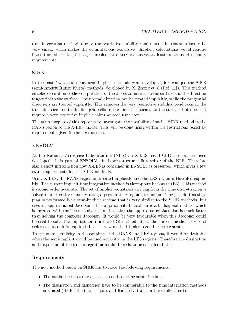
time integration method, due to the restrictive stability conditions , the timestep has to bevery small, which makes the computations expensive. Implicit calculations would requirefewer time steps, but for large problems are very expensive, at least in terms of memoryrequirements.
SIRK
In the past few years, many semi-implicit methods were developed, for example the SIRK(semi-implicit Runge Kutta) methods, developed by X. Zhong et al (Ref [11]). This methodenables separation of the computation of the direction normal to the surface and the directiontangential to the surface. The normal direction can be treated implicitly, while the tangentialdirections are treated explicitly. This removes the very restrictive stability conditions in thetime step size due to the fine grid cells in the direction normal to the surface, but does notrequire a very expensive implicit solver at each time step.
The main purpose of this report is to investigate the useability of such a SIRK method in theRANS region of the X-LES model. This will be done using within the restrictions posed byrequirements given in the next section.
ENSOLV
At the National Aerospace Laboratorium (NLR) an X-LES based CFD method has beendeveloped. It is part of ENSOLV, the block-structured flow solver of the NLR. Thereforealso a short introduction how X-LES is contained in ENSOLV is presented, which gives a fewextra requirements for the SIRK methods.
Using X-LES, the RANS region is threated implicitly and the LES region is threaded explic-itly. The current implicit time integration method is three-point backward (B3). This methodis second order accurate. The set of implicit equations arriving from the time discretisation issolved in an iterative manner using a pseudo timestepping technique. The pseudo timestep-ping is performed by a semi-implicit scheme that is very similar to the SIRK methods, butuses an approximated Jacobian. The approximated Jacobian is a tridiagonal matrix, whichis inverted with the Thomas algorithm. Inverting the approximated Jacobian is much fasterthan solving the complete Jacobian. It would be very favourable when this Jacobian couldbe used to solve the implicit term in the SIRK method. Since the current method is secondorder accurate, it is required that the new method is also second order accurate.
To get more simplicity in the coupling of the RANS and LES regions, it would be desirablewhen the semi-implicit could be used explicitly in the LES regions. Therefore the dissipationand dispersion of the time integration method needs to be considered also.
Requirements
The new method based on SIRK has to meet the following requirements:
• The method needs to be at least second order accurate in time,
• The dissipation and dispersion have to be comparable to the time integration methodsnow used (B3 for the implicit part and Runge-Kutta 4 for the explicit part),

7
• The approximated Jacobian used in the current line-implicit scheme should also workas Jacobian for the SIRK methods,
• The implicit solver has to be an order faster than the method with pseudo timesteps,now used for X-LES.
The requirements will be investigated extensively in this report.
Overview
After this introductory chapter there is a chapter about the theoretical aspect of the semi-implicit methods. Chapter 3 contains a few model problems solved with a semi-implicitmethod and in the end of that chapter a choice has been made for a certain method to beimplemented. Chapter 4 is about the implementation of that method in ENSOLV. Chapter5 contains some standard test cases with the newly implemented method in ENSOLV.

8 CHAPTER 1. INTRODUCTION

Chapter 2
Semi implicit time integrationschemes
2.1 Semi implicit Runge Kutta methods
A theory about semi-implicit Runge-Kutta methods (SIRK) and its low-storage variants(LSSIRK) is introduced by Zhong respectively in reference [11] and reference [10]. In thissection his argumentation is partly followed. As stated in the introduction many problems inCFD have a separable stiff and non-stiff part in their differential equations, which are treatedseparately. The equation du
dt = f(u) is considered an already spatially discretised set of au-tonomous differential equations. The right hand side f will be split in f(u) = f(u) + g(u),where f(u) contains the non-stiff terms and g(u) contains the stiff terms. First some analysison the SIRK schemes is done. The LSSIRK schemes are a special class of SIRK schemes withsome extra restrictions on the coefficients. The most general way to write a r-stage SIRKscheme is,
un+1 = un +r∑
j=1
ωjkj (2.1)
ki = δt
f(un +i−1∑
j=1
bijkj) + g(un +i−1∑
j=1
cijkj + diki)
i ∈ 1, . . . , r.
This scheme is called a method-A scheme. Method-A does not prescribe anything for thetreatment of the implicit term. In method-C1 the implicit term is linearised,
un+1 = un +
r∑
j=1
ωjkj (2.2)
I − δtdiJ(un +
i−1∑
j=1
cijkj)
ki = δt
f(un +
i−1∑
j=1
bijkj) + g(un +
i−1∑
j=1
cijkj)
i ∈ 1, . . . , r.
In these equations, J represents the Jacobian of g.
1it is called method-C and not method-B to be consistent with the notation in most of the literature (eg.reference [11]), method-B is left out because it is not useful in this case
9

10 CHAPTER 2. SEMI IMPLICIT TIME INTEGRATION SCHEMES
2.1.1 Accuracy conditions
First the accuracy conditions for the parameters of both methods are considered. This isdone by comparing the Taylor series of f(u) and g(u) and the Taylor series of the methods.Since third order accuracy is necessary, 3-stage SIRK schemes are considered and the Taylorseries need to be determined up to the third order. This leads to the following conditions:
for first order accuracy for both method-A and method-C:
ω1 + ω2 + ω3 = 1,
for second order accuracy for both method-A and method-C:
ω2b21 + ω3(b31 + b32) =1
2
ω1d1 + ω2(d1 + c21) + ω3(d3 + c32 + c31) =1
2,
for third order accuracy for both method-A and method-C:
ω2(b221) + ω3(b32 + b31) =
1
3
ω3b21b32 =1
6
ω2(b21d2 + b21d1) + ω3(d1b31 + d2b32 + c21b32 + b21c32 + d3b31 + d3b32) =1
3
ω1d21 + ω2(d
22 + d2c21 + d1c21) + ω3(d1c32 + d2c32 + c21c32 + d3c32 + d3c31 + d2
3) =1
6,
an extra condition for method-A third order accuracy:
ω1d21 + ω2(c21 + d2
2) + ω3(c31 + c32 + d3)2 =
1
3,
and an extra condition for method-C third order accuracy
ω2(c221 + 2d2c21) + ω3(c31 + c32)
2 + ω3(2d3(c31 + c32)) =1
3.
When analysing these conditions, a few remarks must be made. At first, when only a secondorder accuracy is required, the same conditions can be used. Set ω3 = 0 and only theconditions for first and second order are considered, and a 2-stage, second order accuracySIRK method is created. As those conditions are the same for method-A and method-C, thesame parameters can be used.
When the first and second order conditions are investigated more thoroughly, it can be seenthat the parameters that represent the explicit part (bij) and those that represent the implicitpart (cij and di) are in different equations. Thus, if only second order accuracy is required,an arbitrary second-order accurate explicit and an arbitrary second-order diagonally-implicitRunge-Kutta scheme can be used to created a SIRK-2A or SIRK-2C method as long as theyhave the same values for ω1 and ω2. When higher order Runge-Kutta schemes are used for
2.1. SEMI IMPLICIT RUNGE KUTTA METHODS 11
this, the result will still be second order, because then the coupling of the implicit and explicitpart comes into play. Before the (LS)SIRK methods were introduced by Zhong, the couplingalways was a problem, and often only second order accurate methods were used. A well-known example of such a method is the Adams-Bashforth/Crank-Nicolson (ABCN) method,which uses Adams-Bashforth for the explicit part and Crank-Nicolson for the implicit part.
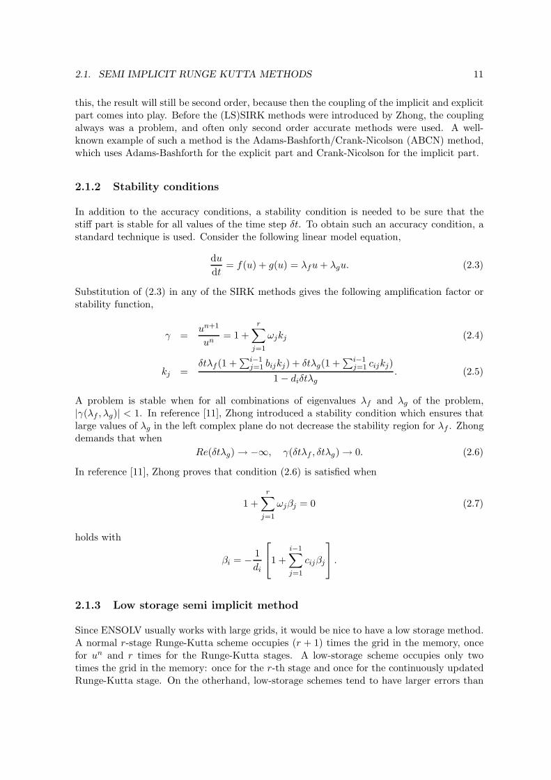
2.1.2 Stability conditions
In addition to the accuracy conditions, a stability condition is needed to be sure that thestiff part is stable for all values of the time step δt. To obtain such an accuracy condition, astandard technique is used. Consider the following linear model equation,
du
dt= f(u) + g(u) = λfu + λgu. (2.3)
Substitution of (2.3) in any of the SIRK methods gives the following amplification factor orstability function,
γ =un+1
un= 1 +
r∑
j=1
ωjkj (2.4)
kj =δtλf (1 +
∑i−1j=1 bijkj) + δtλg(1 +
∑i−1j=1 cijkj)
1 − diδtλg. (2.5)
A problem is stable when for all combinations of eigenvalues λf and λg of the problem,|γ(λf , λg)| < 1. In reference [11], Zhong introduced a stability condition which ensures thatlarge values of λg in the left complex plane do not decrease the stability region for λf . Zhongdemands that when
Re(δtλg) → −∞, γ(δtλf , δtλg) → 0. (2.6)
In reference [11], Zhong proves that condition (2.6) is satisfied when
1 +r∑
j=1
ωjβj = 0 (2.7)
holds with
βi = − 1
di
1 +i−1∑
j=1
cijβj
.
2.1.3 Low storage semi implicit method
Since ENSOLV usually works with large grids, it would be nice to have a low storage method.A normal r-stage Runge-Kutta scheme occupies (r + 1) times the grid in the memory, oncefor un and r times for the Runge-Kutta stages. A low-storage scheme occupies only twotimes the grid in the memory: once for the r-th stage and once for the continuously updatedRunge-Kutta stage. On the otherhand, low-storage schemes tend to have larger errors than

12 CHAPTER 2. SEMI IMPLICIT TIME INTEGRATION SCHEMES
non-low-storage schemes. This will be evaluated during the model problems. The method-Avariant (LSSIRK-rA) looks like:
kj = aj kj−1 + δt[f(uj−1) + g(uj−1 + cj kj−1 + cjkj)
]
uj = uj−1 + bj kj
and the method-C variant (LSSIRK-rC) has the following form:
[I − δtcjJ(uj−1 + cj)] kj = δt[f(uj−1) + g(uj−1 + cj kj−1)
]+ aj [I − δtcjJ(uj−1 + cj)] kj−1
uj = uj−1 + bj kj .
The variable u0 represents un in the normal variant and ur represents un+1. Of course Jrepresents the Jacobian of g again. The product of J and kj−1 is strictly not necessary,but gives better stability regions later on. When the LSSIRK methods are written as SIRKmethods, their conversion parameters can be determined easily. Knowing them, the samestability and accuracy conditions can be used. For a three stage scheme the parametersshould be defined as follows:
for both methods
ω1 = b1 + b2a2 + b3a3a2 b21 = b1 d1 = c1
ω2 = b2 + b3a3 b31 = b1 + b2a2 d2 = c2
ω3 = b3 b32 = b2 d3 = c3
for method-A
c21 = b1 + c2 + c2a2
c31 = b1 + b2a2 + c3a2 + a2c3a2
c32 = b2 + c3 + c3a3
and for method-C
c21 = b1 + c2
c31 = b1 + b2a2 + c3a2
c32 = b2 + c3.
For a two-stage scheme, the parameters which have a subscript three can just be omitted.As can be seen, because of the choice of an extra J in each Runge-Kutta stage, also theparameters for the second step already are different for method-A and method-C.
2.1.4 Parameters for various (LS)SIRK methods
In this section an overview is presented of the sets of parameters found by Zhong et al. forthe method A and method C versions of the third order (LS)SIRK schemes.

2.1. SEMI IMPLICIT RUNGE KUTTA METHODS 13
SIRK−3A
0.4
0.6
0.6
0.6
0.8
0.8
0.80.81
1
1
1
Re(λf h)
Im(λ
f h)
−3 −2 −1 00
0.5
1
1.5
2SIRK−3C
0.4
0.6
0.6
0.6
0.8
0.80.8
11
1
1Re(λ
f h)
Im(λ
f h)
−3 −2 −1 00
0.5
1
1.5
2LSSIRK−3C
0.4
0.6
0.6
0.60.8
0.8
0.8
1
1
1
Re(λf h)
Im(λ
f h)
−3 −2 −1 00
0.5
1
1.5
2
Figure 2.1: Stability regions of SIRK-3A, SIRK-3C and LSSIRK-3C
SIRK-3A
w1 = 18 b21 = 8
7 d1 = 34 c21 = 5589
6524w2 = 1
8 b31 = 71252 d2 = 75
233 c31 = 769126096
w3 = 34 b32 = 7
36 d3 = 65168 c32 = −26335
78288
SIRK-3C
ω1 = 18 b21 = 8
7 d1 = 0.7970967740096232 c21 = 1.058925354610082ω2 = 1
8 b31 = 71252 d2 = 0.5913813968007854 c31 = 1
2ω3 = 3
4 b32 = 736 d3 = 0.1347052663841181 c32 = −0.3759391872875334
LSSIRK-3C
b1 = 14 a2 = −1
4 c2 = −1.143097033946135 c1 = 2.267596813284564b2 = 2
9 a3 = −2927 c3 = −2.031219208388789 c2 = 2.685297589634163
b3 = 3 c3 = 2.309749357551431
The LSSIRK-3A method is not included, although it was tested during the stability tests.The parameters Zhong gave, did not statisfy the stability condition (2.7). The larger theabsolute value of λg became, the larger the absolute value of γ grew.
2.1.5 Stability regions
The stability regions of the considered methods are presented in this section. The stabilityregion plots are based on the theory in section 2.1.2. For plotting these stability regions, themaximum absolute value of γ is computed for each λf over λg in the left complex plane. Theresults are shown in figure 2.1.
All three methods have an acceptable stability region. They all contain a part of the imaginaryaxis, which is important because the eigenvalues of high Reynolds number flows as appearin ENSOLV lie close to the imaginary axis. LSSIRK-3C seems to be the best, because itincludes the largest part of the imaginary axis and even permits small positive values of λf
near the imaginary axis.

14 CHAPTER 2. SEMI IMPLICIT TIME INTEGRATION SCHEMES
2.1.6 Dissipation and dispersion
It is not only important that a method is stable, as discussed in section 2.1.2, a method shouldalso have an acceptable dissipation (non physical damping) and dispersion (the phase error).Dissipation and dispersion is usually defined as described below. When γ is the amplificationfactor of the method and γex the exact amplification factor of the one dimensional version of(2.3), the quotient of both is considered in the following manner:
γ
γex= |r|eiφ,
where r is the dissipation and φ the dispersion. The exact solution for a problem has dissi-pation r one and the dispersion φ zero. The dissipation should always be less or equal thanone, otherwise the problem is not stable. It is possible to create dissipation and dispersionfigures with this definition, not considering the dissipation and the dispersion created by aspatial discretisation. For central convection discretisations, for example, it is usual to lookat the dispersion and dissipation on the upper imaginary axis, so λf , λg ∈ [0,∞]i.
Spatial discretisation
If the spatial discretisation is considered , some extra work needs to be done. Consider theconvection differential equation
∂u
∂t+
∂cu
∂x= 0, c > 0 (constant), x ∈ [0, L], t > 0 (2.8)
u(x, 0) = Ueikx, k =2π
l,
u(0, t) = u(L, t)
with L the wave length and k the wave number of the initial solution, which has the solution
u(x, t) = Ueik(x−ct) = Uei(kx−ωt) = u(t)eikx,
with u(t) = Ue−iωt and ω = ck. The time of one period will be written as T = 2πω = l
c .
The spatial discretisation is defined arbitrary as long as it fits in the following semi-discretisedform of the differential equation,
xj = jδx, j = 0 . . . N, δx =L
Nduj
dt=
c
δx
∑
m
αmuj+l (2.9)
Fourier analysis
The discrete solution for uj = u(jδx, t) can be written as (analogous to the exact solution),
uj = ueikxj = ueiθj

2.1. SEMI IMPLICIT RUNGE KUTTA METHODS 15
with θ = kδx = 2πδxl = ωδx
c . θ is the wave number in the computational domain. Substitutingthe latter into equation (2.9) and dividing by eiθj gives:
du
dt=
c
δx
∑
m
αmeiθmu =c
δxz(θ)u = ω
z(θ)
θu
with z(θ) =∑
m αmeiθm. The latter equation can be solved with a time integration methodand divided by the exact solution for (2.8) to determine the dispersion and the dissipation ofthe spatial and time integration combined.
When the dissipation and dispersion rate of both the implicit and explicit part of a (LS)SIRKneeds to be determined, one spatial dimension in (2.8) is not sufficient. It is fairly easy toadd an extra spatial dimension y in (2.8),
∂u
∂t+
∂cxu
∂x+
∂cyu
∂y= 0, cx, cy > 0 (constant), x, y ∈ [0, Lx] × [0, Ly ], t > 0
u(x, y, 0) = Uei(kxx+kyy), kx =2π
lx, ky =
2π
ly
u(0, 0, t) = u(Lx, Ly, t)
which has the solution
u(x, t) = Uei(kx(x−cxt)+ky(y−cyt)) = Uei(kxx−ωxt+kyy−ωyt) = u(t)ei(kxx+kyy),
with u(t) = e−i(ωx+ωy)t, ωx = cxkx and ωy = cyky. After doing the same steps as done withthe one dimensional version the following equation for u is found
du
dt=
cx
δxz(θx) +
cy
δyz(θy)
u =
ωx
z(θx)
θx+ ωy
z(θy)
θy
u.
Comparing the spatial discretised version with the exact solution
When the discretised versions are compared, the CFL number cδtδx is kept constant and θ is
varied. This can be done in two ways. The first way is to fix the mesh (δx is constant) andvary the wave number k. Then e.g. after one time step δt the quotient of the amplificationfactors of the discretised version and the exact solution can be considered as a function of thewave number k.
The second way is to vary the mesh and fix the wave number. In this way the number of gridcells to accurately capture a wave length can be easily determined. Some more work is neededfor this one. Since the CFL number is fixed and δx is varying, also δt has to vary. Let Nx
be the varying number of grid cells per wave length, Nx = lδx . Now the computational wave
number can be written as θ = 2πNx
. Nt = Tδt represents the number of time steps needed for
one period T. Knowing that c = lT , the CFL number can be written as CFL = δt/T
δx/l = Nx
Nt.
Consider the amplification factors after a fixed time span T , which has in the discretisedversion a varying number of time steps Nt = Nx
CFL = 2πCFLθ depending on the wave number in
the computational domain θ.

16 CHAPTER 2. SEMI IMPLICIT TIME INTEGRATION SCHEMES
0 0.2 0.40.99
0.992
0.994
0.996
0.998
1
iλf*δ t
Dis
sapt
ion
rate
|r|
0 0.2 0.4
0
0.01
0.02
0.03
0.04
iλfδ t
Pha
se e
rror
φ
RealRunge−Kutta 4B3(LS)SIRK−3A/C
RealRunge−Kutta 4B3(LS)SIRK−3A/C
Figure 2.2: Dispersion and dissipation of various methods: time discretisation only
0 0.5 1 1.50.8
0.85
0.9
0.95
1
θ
Dis
sapt
ion
rate
|r|
0 0.5 1 1.50
0.1
0.2
0.3
0.4
0.5
0.6
θ
Pha
se e
rror
φ
RealRunge−Kutta 4B3(LS)SIRK−3A/C
RealRunge−Kutta 4B3(LS)SIRK−3A/C
Figure 2.3: Dispersion and dissipation of various methods: time and space discretisationcompared by varying k
0 20 400.5
0.6
0.7
0.8
0.9
1
N
Dis
sapt
ion
rate
|r|
0 20 400
2
4
6
8
10
N
Pha
se e
rror
φ
RealRunge−Kutta 4B3(LS)SIRK−3A/C
RealRunge−Kutta 4B3(LS)SIRK−3A/C
Figure 2.4: Dispersion and dissipation of various methods: time and space discretisationcompared by varying the number of grid cells per wave length Nx

2.1. SEMI IMPLICIT RUNGE KUTTA METHODS 17
b3: dissipation rate |r| (cflx,cfl
y) = (100,0.3)
0.9996
0.9997
0.9998
0.9999
0.9999
θx
θ y
0 0.2 0.4 0.6 0.8 1
x 10−3
0
0.05
0.1
0.15
0.2
0.25
0.3
0.35
0.9994
0.9995
0.9996
0.9997
0.9998
0.9999
1b3: phase error φ (cfl
x,cfl
y) = (0.3,100)
0.0005
0.0005
0.001
0.001
0.0015
0.0015
0.0020.0025
0.003
θx
θ y
0 0.2 0.4 0.6 0.8 1
x 10−3
0
0.05
0.1
0.15
0.2
0.25
0.3
0.35
0
0.5
1
1.5
2
2.5
3
3.5
4x 10
−3
Figure 2.5: Dispersion and dissipation of an implicit and explicit direction of B3: time andspace discretisation compared by varying k
2.1.7 Dissipation and dispersion figures
Explicit direction only
When a (LS)SIRK method is used in an X-LES model, it is likely that the explicit LESareas are also solved with a LS(SIRK) method. This is convenient because of the couplingof the explicit LES and semi-implicit RANS areas. Therefore it is necessary to compare thedissipation and dispersion of the explicit part of the (LS)SIRK methods with the methodsnow used in ENSOLV’s X-LES model: second order backward (B3) and Runge-Kutta 4.
Figures 2.2 to 2.4 show the comparisons described in the previous section using CFL = 1.Figure 2.2 represents the dispersion and dissipation of the one dimensional version of (2.3).Figures 2.2 and 2.3 respresent the convection equation (2.8) with a fourth order central spatialdiscretisation: the middle one with a varying wave number, the lower one with a varyingnumber of grid cells per wave length.
The first remark that has to be made is that the results for LSSIRK-3C, SIRK-3C and SIRK-3A are the same. This is because the explicit parts of those methods use exactly the samecoefficients. It was expected that the results of the third order (LS)SIRK methods should besomewhere between the second order B3 results and the fourth order Runge-Kutta 4 results.The (LS)SIRK results are much closer to the Runge-Kutta four results than to the B3 results,which is what was hoped for. In figure 2.4 can be seen, that per wave length twice the numberof time steps are needed for the (LS)SIRK methods to get the same dispersion and dissipationon the same grid. Since CFL = 1, N in the figures also represents the number of time stepsper wave length. With these figures it is expected that, from a dispersion and dissipationpoint of view, the (LS)SIRK methods are appropriate for the explicit LES part of a X-LESmodel.

18 CHAPTER 2. SEMI IMPLICIT TIME INTEGRATION SCHEMES
b3: dissipation rate |r| (cflx,cfl
y) = (100,0.3)
0.450.5
0.50.55
0.550.6
0.60.65
0.650.7
0.70.75
0.750.8
0.80.85
0.85
0.9
0.90.9
0.95
0.950.95
0.95 0.95
Number of grid cells per wave length in implicit direction
Num
ber
of g
rid c
ells
per
wav
e le
ngth
in e
xplic
it di
rect
ion
0.5 1 1.5 2 2.5 3
x 104
10
20
30
40
50
60
70
80
90
100
0.45
0.5
0.55
0.6
0.65
0.7
0.75
0.8
0.85
0.9
0.95b3: phase error φ (cfl
x,cfl
y) = (0.3,100)
11
1 1
22
2 23 34 45 56
Number of grid cells per wave length in implicit direction
Num
ber
of g
rid c
ells
per
wav
e le
ngth
in e
xplic
it di
rect
ion
0.5 1 1.5 2 2.5 3
x 104
10
20
30
40
50
60
70
80
90
100
0.5
1
1.5
2
2.5
3
3.5
4
4.5
5
5.5
6
Figure 2.6: Dispersion and dissipation of an implicit and explicit direction of B3: time andspace discretisation compared by the number of gridcells per wave length
sirk3a: dissipation rate |r| (cflx,cfl
y) = (100,0.3)
1
1
1
1
1
1
1
1
1 1
θx
θ y
0 0.2 0.4 0.6 0.8 1
x 10−3
0
0.05
0.1
0.15
0.2
0.25
0.3
0.35
1
1
1
1
1
1
1sirk3a: phase error φ (cfl
x,cfl
y) = (0.3,100)
1e−05
2e−05
3e−054e−055e−056e−05
7e−058e−059e−05
θx
θ y
0 0.2 0.4 0.6 0.8 1
x 10−3
0
0.05
0.1
0.15
0.2
0.25
0.3
0.35
0
1
2
3
4
5
6
7
8
9x 10
−5
Figure 2.7: Dispersion and dissipation of an implicit and explicit direction of SIRK-3A: timeand space discretisation compared by varying k

2.1. SEMI IMPLICIT RUNGE KUTTA METHODS 19
sirk3a: dissipation rate |r| (cflx,cfl
y) = (100,0.3)
0.75
0.75
0.8
0.8
0.85
0.85
0.9
0.9
0.95
0.95
1
1
1
1
Number of grid cells per wave length in implicit direction
Num
ber
of g
rid c
ells
per
wav
e le
ngth
in e
xplic
it di
rect
ion
0.5 1 1.5 2 2.5 3
x 104
10
20
30
40
50
60
70
80
90
100
0.7
0.75
0.8
0.85
0.9
0.95
1sirk3a: phase error φ (cfl
x,cfl
y) = (0.3,100)
1 12 23 34 45 56
Number of grid cells per wave length in implicit direction
Num
ber
of g
rid c
ells
per
wav
e le
ngth
in e
xplic
it di
rect
ion
0.5 1 1.5 2 2.5 3
x 104
10
20
30
40
50
60
70
80
90
100
0.5
1
1.5
2
2.5
3
3.5
4
4.5
5
5.5
6
Figure 2.8: Dispersion and dissipation of an implicit and explicit direction of SIRK-3A: timeand space discretisation compared by the number of gridcells per wave length
Implicit and explicit direction
Ofcourse, also the dispersive and dissipative behaviour of the (LS)SIRK methods have tobe considered in the RANS, semi-implicit, areas of the problem. Therefore, also some twodimensional plots are made considering both the implicit and explicit direction of the method.To simulate the high aspect ratios of the grid cells typically found in the RANS area, theCFL number in the implicit direction is more than three hunderd times larger than the CFLnumber in the explicit direction. Just as in the previous figures the methods are comparedwith the methods already present in ENSOLV. Because of the high CFL number, it is notpossible to compare the results with explicit Runge-Kutta methods, so only the second orderbackward (B3) is considered. To avoid too much figures in the report, only time and spacediscretisation together are considered. First with varying wave number k and secondly with avarying number of grid cells per wave length. Since the results of all (LS)SIRK methods arealmost the same, only the results of SIRK-3A will be shown. In the figures a CFL number of0.3 in the explicit direction is used, this is because the central spatial discretisation has pureimaginary eigenvalues and is not stable for pure imaginary eigenvalues greater than about0.35 . In practice the eigenvalues have small negative parts due to the artificial dissipationand the diffusive term, so CFL numbers up to 1.5 can be used. More about this can be foundin section 2.1.2.
Figures 2.5 to 2.8 show the results. Both B3 and SIRK-3A are almost symmetric in the line θx
= θy in the dissipation figures. Knowing this, the same conclusions can be made as with theone dimensional dissipation figures. The dissipation of the SIRK-3A method is significantlysmaller than the dissipation of the B3 method. Also the dispersion of the SIRK-3A schemeis smaller than the dispersion of the B3 scheme. From a dissipation and dispersion point ofview, (LS)SIRK methods are very suitable for the RANS areas.

20 CHAPTER 2. SEMI IMPLICIT TIME INTEGRATION SCHEMES
2.2 The implicit term
To be able to use an A variant (as described in equation (2.1)) of a (LS)SIRK method, amethod to solve the implicit term needs to be determined. There are a number of possibilities.Three are considered here.
2.2.1 Exact solution
The first one is to determine an exact solution of the implicit equation. This can be veryexpensive, because in ENSOLV and a few of the test cases this is a set of non-linear equations.This method can be used for example to determine a reference solution to which the othermethods can be compared. In practice for model problems in MATLAB, a builtin non-linearequation solver can be used.
2.2.2 Linearised
The second one, a quite simple one, is to use the method used in the C variants as describedin equation (2.2). A difference between the A and C variant is that the coefficients in the Avariants are choosen in such a way that an exact solution of the implicit term is expected,while in the C variants the coefficients are choosen such that only this linearisation is consid-ered. With non-linear problems it is expected that this treatment of the implicit term is notsufficient for the A variants.
2.2.3 The Newton method for solving a system of non-linear equations
The Newton method is described more extensively. The Newton method for system of non-linear equations is a generalisation of the Newton method for the one-dimensional case forsolving h(x) = 0. The one-dimensional case can be described by the following fixed-pointmethod:
x(l) = x(l−1) − φ(x(l−1))h(x(l−1)),
where φ(x) = 1/h′(x). In for example reference [1] this method is derived and there is alsoproven that this method has quadractic convergence to h(x) = 0 when the initial estimationx(0) is close enough to the real root.
The multi-dimensional case for solving H(x) = 0, where x and H is a vector now, can beconstructed by replacing h′(x) with the Jacobian of H(x) denoted as K(x). Which results in:
x(l) = x(l−1) − K−1(x(l−1))H(x(l−1)).
Again a proof of quadratic convergence when the initial estimation x(0) is close enough to thereal root is given in reference [1].

2.2. THE IMPLICIT TERM 21
The Newton methods for (LS)SIRK-rA
Now H(x) and K(x) will be determined for a Runge-Kutta stage in a (LS)SIRK-rA method.First the equation to be solved for each Runge-Kutta stage, equation (2.1), is recalled:
ki = δt
f(un +i−1∑
j=1
bijkj) + g(un +i−1∑
j=1
cijkj + diki)
.
So each Runge-Kutta stage x := ki is the variable to be solved, which leads to
H(x) = x − δt
f(un +i−1∑
j=1
bijkj) + g(un +i−1∑
j=1
cijkj + dix)
,
where all the other variables and functions are known. The Jacobian matrix of H(x) can bedetermined now:
K(x) = I − δtdiJ(un +
i−1∑
j=1
cijkj + dix),
where I is the N -dimensional identity matrix, J the Jacobian matrix of g, N the dimensionof the vector x and n the indicator of the previous time step.
Two things additionally need to be considered. First what initial estimate x(0) is used. Sinceki represents a part of the difference between two succesive time steps and the time steps aresmall, it will be assumed that the difference is not so big and x(0) = 0 is close enough to thereal difference between two succesive time steps.
Furthermore a stopping criterion is needed. Two kinds of stopping criteria are used in themodel problems. The first one is to stop the Newton method after a fixed number of steps.The second one is to stop the Newton method at step l when ‖H(x(l))‖ or ‖x(l) − x(l−1)‖ issmaller than a certain tolerance ε. The drawback of using the easier ‖x(l) −x(l−1)‖ ≤ ε is thatwhen two succesive Newton steps are close to each other but not to the root of H(x) it alsostops. That is why ‖H(x(l))‖ ≤ ε or a combination of both is used.
In order to be able to compare different time step sizes with the same base tolerance ε∗, ε isscaled with the time step size (δt)s, where s is the order of convergence of the time integrationmethod. So the residue of the Newton method stays scales with the error introduced by thetime integration method. When ‖x‖ is not of order one, ε can also be scaled with ‖x‖.Resulting in
ε = ε∗(δt)s‖xk−1‖. (2.10)
A major drawback of the Newton method is that, unlike for example the bisection method,it does not always converge to the nearest root. On the other hand, in the derivation of theNewton method it can be seen that the Jacobian can be approximated in stead of determinedexactly as presumably needed in the C variant methods. In the test cases in the next chapterit will be determined whether the Newton method with x(0) = 0 works as non-linear solverfor the implicit part of (LS)SIRK-rA methods.

22 CHAPTER 2. SEMI IMPLICIT TIME INTEGRATION SCHEMES
2.3 Computational efforts
In this section the theorical computational effort for ENSOLV for the current method andfor the different (LS)SIRK methods are determined. In the next chapter, when for examplethe number of Newton steps in the Newton method are known, a comparison in speed canbe made. The comparison is based on the number of residual computations that are madein the implicit block and explicit block and the number of approximated Jacobian inversionsthat are made in the implicit block. The computation effort in time of an implicit block, anexplicit block and a Jacobian inversion are represented by respectively Ri,Re and Ii.
2.3.1 Current line-implicit method with coupling
In the current scheme each physical time step Np pseudo time steps with N is Runge-Kutta
stages are done in the implicit block, in each of the Runge-Kutta stages one residual iscomputed and one approximated Jacobian inversion is done. In the explicit part N e
s Runge-Kutta stages are done, each of those steps one residual is computed. This leads to a totalof
Ccurrent = NpNis(Ri + Ii) + N e
s Re
computations per physical time step.
2.3.2 (LS)SIRK methods
The (LS)SIRK methods are divided in two groups. First SIRK-3A with the implicit termlinearised, SIRK-3C and (LS)SIRK-3C, they all require one approximated Jacobian inversionand one residual computation for the implicit block. The same method is used for the explicitblock, but then only the residual computation is needed. Each physical timestep N s
s Runge-Kutta stages are taken, which gives a total of
Csirk = N ss (Ri + Re + Ii)
computations per physical time step. Secondly, when the Newton method is used for theimplicit term each Runge-Kutta stage Nn Newton steps are needed to compute the implicitterm. Which gives a total of
Csirknewton = N ss (Nn(Ri + Ii) + Re)
computations per physical time step.
2.3.3 Comparison
It is hard to compare the current line-implicit method and the (LS)SIRK methods. The timestep sizes needed for a reasonable answer can be different as was shown in the dispersion anddissipation figures. For different problems the computational ratio between the implicit andexplicit block are not the same and the number of Newton steps needed for a Newton basedSIRK method is not known. A few example cases are compared.

2.4. DISCUSSION 23
Totally implicit with the same grid size
Now Re = 0, which leads to Csirknewton = NnCsirk. So using a non-Newton (LS)SIRKmethod is Nn times cheaper than using a SIRK-3A with Newton. Also Ri and Ii are thesame for the current method and the (LS)SIRK methods. Which gives the following ratio,
γimp =Ccurrent
Csirknewton=
NpNis
NnN ss
. (2.11)
Usually N is = 5, Np = 100 and since in this report only 3 stage (LS)SIRK methods are
considered N ss = 3. If the approximated Jacobian inversion are accurate enough for the non
Newton methods (Nn = 1), γimp ≈ 167, so those methods would be 167 times faster thanthe current line-implicit method. Since Nn is not known yet, approximations for SIRK-3Awith Newton will be made in the next chapter.
Coupling test case
In reference [7] Scheijbeler, did a test run with the current line implicit method. The per-formance results of that test case can be found on page 87 of reference [7]. Those resultsare used now to compare the theorical speed of the (LS)SIRK methods and the current lineimplicit method with coupling. From Scheijbelers results can be derived that for the currentmethod and that test case Ri + Ii ≈ Re. Scheijbeler used Np = 50 pseudo time steps andN i
s = 5 and N es = 4 Runge-Kutta stages. Again it is assumed that N s
s = 3. Using the samegrid size for the (LS)SIRK methods, now the following ratio is obtained,
γcoup =Ccurrent
Csirknewton=
NpNis + N e
s
(Nn + 1)N ss
≈ 85
Nn + 1. (2.12)
When the non-Newton methods work, so Nn = 1, γcoup ≈ 43. The estimates made forSIRK-3A with the Newton method are made in the next chapter.
2.4 Discussion
Three methods discussed in this chapter are worth trying in the test cases: LSSIRK-3C,SIRK-3A and SIRK-3C. Low storage methods are preferred above non low storage methods,because they use less memory. The C variant methods are most likely quicker than the Avariant methods because per Runge-Kutta only one time the Jacobian has to be inverted,while in the A methods a non-linear system of equations has to be solved. In section 2.2 afew methods for treating this implicit term are introduced, where solving it exact is an optionfor the simple test problems, but not for the more complicated problems typically solved byENSOLV, because the expense in terms of computer time. Only linearising the term andsolving that, will most likely not give third order results for non-linear problems. So theNewton method is in practice the only option left from the three.
In terms of memory use and computer time LSSIRK-3C is the most interesting method,providing it performs well with an approximated Jacobian. Followed by SIRK-3C with thesame requirement with respect to the Jacobian. Most likely SIRK-3A in combination with

24 CHAPTER 2. SEMI IMPLICIT TIME INTEGRATION SCHEMES
the Newton method will work for approximated Jacobians, at the cost of an iterative processeach Runge-Kutta stage.
In the next chapter it will be evaluated,
• whether the methods converge third order,
• how sensitive the Newton method and the C variants are for approximating Jacobians(as used in ENSOLV)
• and which parameters and how many steps are needed for the Newton method to con-verge.

Chapter 3
Testing (LS)SIRK methods onmodel problems
3.1 Model problem: Convection-diffusion equation
For analysing semi-implicit time integration methods a model is needed that,
• has an exact solution, that can be determined,
• can be split in a stiff part in one direction and a non stiff part in another direction,
• has some sort of ‘difficulty’ at one of the boundaries,
• is a time dependent problem,
and since it is a model problem, it has to be as simple as possible.
A suitable problem is the convection-diffusion equation
∂u
∂t+ R = 0
with
R = div(a u − µ grad u)
and a a vector which contains the convective velocities. When the incompressibility condition(div a = 0) is assumed, the equation can be written with R in its more common form
R = a grad u − div(µ grad u).
The two dimensional version of this equation for u(x, y, t) on the region x, y ∈ [0, 1] × [0, 1]and t ∈ [0,∞] can be writen as
∂u(x, y, t)
∂t= µ
∂2u(x, y, t)
∂y2− a
∂u(x, y, t)
∂x− b
∂u(x, y, t)
∂y(3.1)
25

26 CHAPTER 3. TESTING (LS)SIRK METHODS ON MODEL PROBLEMS
with the following initial and boundary conditions
u(x, 0, t) = 0 (3.2)
u(x, 1, t) = 1 (3.3)
u(0, y, t) = u(1, y, t) (3.4)
u(x, y, 0) = f(x, y) (3.5)
The y-direction is considered to be the stiff one. The x-direction is the non-stiff one. To makethe x-direction even less stiff and to avoid any numerical restrictions, the diffusion constantin that direction is zero.
3.1.1 Analytical solution
The problem is not homogeneous, which makes it more difficult to solve. On physical groundsit is assumed that the solution will converge in time to a time steady solution,
S(y) = limt→∞
u(x, y, t),
which is also constant in the x-direction. The solution can be written as u(x, y, t) = S(y) +v(x, y, t). Under those assumptions the boundary conditions for u(x, y, t) can be rewritten forv(x, y, t) and will become
v(x, 0, t) = v(x, 1, t) = 0 (3.6)
v(0, y, t) = v(1, y, t) (3.7)
v(x, y, 0) = f(x, y) − S(y) (3.8)
The time steady solution
First the solution for S(y) will be determined. Since S(y) only depends on y and is timeindependent, the equations simplify to
b∂S
∂y− µ
∂2S
∂y2= 0
with S(0) = 0 and S(1) = 1. The solution of this problem is given for example in reference[8] and is
S(y) =1 − e−
bµ
y
1 − e−
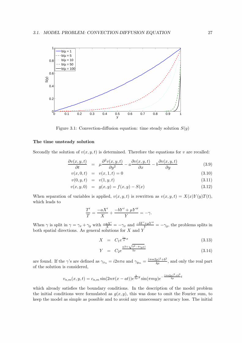
bµ
.
Figure 3.1 shows that for bµ 1 the solution has a small boundary layer at y = 1, which is
desirable for the model problem.
3.1. MODEL PROBLEM: CONVECTION-DIFFUSION EQUATION 27
0 0.1 0.2 0.3 0.4 0.5 0.6 0.7 0.8 0.9 10
0.2
0.4
0.6
0.8
1
y
S(y
)
b/µ = 1b/µ = 5b/µ = 10b/µ = 50b/µ = 100
Figure 3.1: Convection-diffusion equation: time steady solution S(y)
The time unsteady solution
Secondly the solution of v(x, y, t) is determined. Therefore the equations for v are recalled:
∂v(x, y, t)
∂t= µ
∂2v(x, y, t)
∂y2− a
∂v(x, y, t)
∂x− b
∂v(x, y, t)
∂y(3.9)
v(x, 0, t) = v(x, 1, t) = 0 (3.10)
v(0, y, t) = v(1, y, t) (3.11)
v(x, y, 0) = g(x, y) = f(x, y) − S(x) (3.12)
When separation of variables is applied, v(x, y, t) is rewritten as v(x, y, t) = X(x)Y (y)T (t),which leads to
T ′
T=
−aX ′
X+
−bY ′ + µY ′′
Y= −γ.
When γ is split in γ = γx + γy with −aX′
X = −γx and −bY ′+µY ′′
Y = −γy, the problems splits inboth spatial directions. As general solutions for X and Y
X = C1eγxa
x (3.13)
Y = C2ey(b+
√b2−4γyµ)
2µ (3.14)
are found. If the γ’s are defined as γxn = i2nπa and γym = (πm2µ)2+b2
4µ , and only the real partof the solution is considered,
vn,m(x, y, t) = cn,m sin(2nπ(x − at))eb2µ
ysin(πmy)e
−(πn2µ)2+b2
4µt
which already satisfies the boundary conditions. In the description of the model problemthe initial conditions were formulated as g(x, y), this was done to omit the Fourier sum, tokeep the model as simple as possible and to avoid any unnecessary accuracy loss. The initial

28 CHAPTER 3. TESTING (LS)SIRK METHODS ON MODEL PROBLEMS
condition g(x) can be defined in such a way that for only one value of n and m, v(x, y, t)satisfies the initial conditions. When g(x, y) is of the form
g(x, y) = S(y) + C sin(2nπx)eb
2µysin(2mπy),
in v only the n-th node for the x-direction has to be computed and only the m-th for they-direction.
Solution for u(x, y, t)
Combining this information gives the full solution for u(x, y, t) and a useable form for theinitial condition f(x)
u(x, y, t) = cn,m sin(2nπ(x − at))eb2µ
ysin(2πmy)e
−(πn2µ)2+b2
4µt+
1 − ebµ
x
1 − ebµ
(3.15)
f(x, y) =1 − e
bµ
y
1 − ebµ
+ C sin(2nπ(xk − at))eb2µ
ysin(2mπy) (3.16)
This exact solution is used to check the accuracy of the time integration method.
3.1.2 Spatial discretisation
For simplicity reasons a uniform grid is used. Because ENSOLV works cell-centered, thereforethis discretisation will also be cell-centered. The number of grid cells in the x direction iscalled nx, the number of grid cells in the y-direction is called ny.
The values in the grid cells center are defined as ui,j(t) = u((12 +i)k, (1
2 +j)l, t) for i ∈ 1, . . . , nx
and j ∈ 1, . . . , ny, with k = 1/nx and l = 1/ny. Figure 3.2 shows a graphical representationof the grid.
For linear problems on a uniform grid FDM (finite difference methods) and FVM (finitevolume methods) give the same spatial discretisation schemes, here a FDM method is usedto determine the spatial discretisation. Since the time integration method has to be at leastsecond order, also third order time integration methods will be analysed. When a second orderspatial discretisation is used, the error in time, for small timesteps, will be much smaller thanthe error in space, which is not useful when the approximated solution is compared with theexact solution. A fourth order central method in both directions will be used instead. Thisgives rise to the following 9-point stencil,
r
r
r
r
r
r r r r rf
ui,j−2
ui,j−1
ui,j
ui,j+1
ui,j+2
ui−2,j ui−1,j ui+1,j ui+2,j

3.1. MODEL PROBLEM: CONVECTION-DIFFUSION EQUATION 29
tu1,1
tunx,1
tu1,ny
tunx,ny
- x
6
y
Figure 3.2: Convection-diffusion equation: grid
This leads to the standard central fourth order discretisation (the t’s will be omitted)
(1 + 30µ12l2
)ui,j = bl−µ12l2
ui,j+2 + −8bl+16µ12l2
ui,j+1
+ 8bl+16µ12l2 ui,j−1 + −bl−µ
12l2 ui,j−2
+ a12k ui+2,j + −8a
12k ui+1,j
+ 8a12k ui−1,j + −a
12k ui−2,j
for i = 1, . . . , nx and j = 3, . . . , ny − 2. Due to the periodic boundary conditions in thex-direction, the solutions near those boundaries can be defined as u−1,j ≡ uny−2,j and u0,j ≡uny−1,j .
At the Dirichlet boundaries some more work is needed. The discretisation stencil for two andone cells from the upper boundary is defined as shown below,
t
t
t
t
t t t t tf
t
ui,j−2
ui,j−1
ui,j
ui,j+1
ui,j+1 12
ui−2,j ui−1,j ui+1,j ui+2,jt
t
tt t t t tft
ui,j−2
ui,j−1
ui,j
ui,j+ 12
ui−2,j ui−1,j ui+1,j ui+2,j
.
The stencils for the lower boundaries can be defined in the same way. In section 2.4 fromreference [9] it is shown how to derive the parameters for a discretisation scheme, using thatinformation the following difference equations at the Dirichlet boundaries are determined:
30 CHAPTER 3. TESTING (LS)SIRK METHODS ON MODEL PROBLEMS
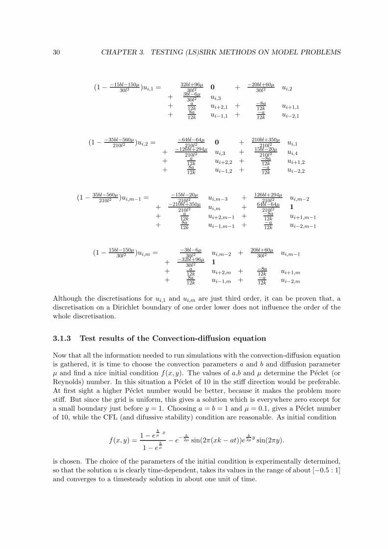
(1 − −15bl−150µ30l2
)ui,1 = 32bl+96µ30l2
0 + −20bl+60µ30l2
ui,2
+ 3bl−6µ30l2
ui,3
+ a12k ui+2,1 + −8a
12k ui+1,1
+ 8a12k ui−1,1 + −a
12k ui−2,1
(1 − −35bl−560µ210l2
)ui,2 = −64bl−64µ210l2
0 + 210bl+350µ210l2
ui,1
+ −126bl+294µ210l2
ui,3 + 15bl−20µ210l2
ui,4
+ a12k ui+2,2 + −8a
12k ui+1,2
+ 8a12k ui−1,2 + −a
12k ui−2,2
(1 − 35bl−560µ210l2
)ui,m−1 = −15bl−20µ210l2
ui,m−3 + 126bl+294µ210l2
ui,m−2
+ −210bl+350µ210l2
ui,m + 64bl−64µ210l2
1+ a
12k ui+2,m−1 + −8a12k ui+1,m−1
+ 8a12k ui−1,m−1 + −a
12k ui−2,m−1
(1 − 15bl−150µ30l2
)ui,m = −3bl−6µ30l2
ui,m−2 + 20bl+60µ30l2
ui,m−1
+ −32bl+96µ30l2
1+ a
12k ui+2,m + −8a12k ui+1,m
+ 8a12k ui−1,m + −a
12k ui−2,m
Although the discretisations for ui,1 and ui,m are just third order, it can be proven that, adiscretisation on a Dirichlet boundary of one order lower does not influence the order of thewhole discretisation.
3.1.3 Test results of the Convection-diffusion equation
Now that all the information needed to run simulations with the convection-diffusion equationis gathered, it is time to choose the convection parameters a and b and diffusion parameterµ and find a nice initial condition f(x, y). The values of a,b and µ determine the Peclet (orReynolds) number. In this situation a Peclet of 10 in the stiff direction would be preferable.At first sight a higher Peclet number would be better, because it makes the problem morestiff. But since the grid is uniform, this gives a solution which is everywhere zero except fora small boundary just before y = 1. Choosing a = b = 1 and µ = 0.1, gives a Peclet numberof 10, while the CFL (and difussive stability) condition are reasonable. As initial condition
f(x, y) =1 − e
bµ
x
1 − ebµ
− e−b
2µ sin(2π(xk − at))eb
2µy sin(2πy).
is chosen. The choice of the parameters of the initial condition is experimentally determined,so that the solution u is clearly time-dependent, takes its values in the range of about [−0.5 : 1]and converges to a timesteady solution in about one unit of time.

3.1. MODEL PROBLEM: CONVECTION-DIFFUSION EQUATION 31
00.5
1
0
0.5
1−0.5
0
0.5
1
x
t=0s
y
Uex
act
00.5
1
0
0.5
1−0.5
0
0.5
1
x
t=0.125s
yU
exac
t
00.5
1
0
0.5
1−0.5
0
0.5
1
x
t=0.25s
y
Uex
act
00.5
1
0
0.5
1−0.5
0
0.5
1
x
t=0.375s
y
Uex
act
00.5
1
0
0.5
1−0.5
0
0.5
1
x
t=0.5s
y
Uex
act
00.5
1
0
0.5
1−0.5
0
0.5
1
x
t=1s
y
Uex
act
Figure 3.3: Convection-diffusion equation: exact solution of the problem
32 CHAPTER 3. TESTING (LS)SIRK METHODS ON MODEL PROBLEMS
10 20 40 60 80 100 120 140 16010
−6
10−5
10−4
10−3
10−2
10−1
timesteps per second
Max
. abs
. err
or
LSSIRK−3CSIRK−3CSIRK−3AO(h)O(h2)O(h3)
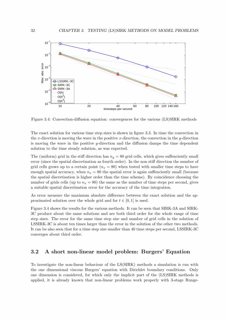
Figure 3.4: Convection-diffusion equation: convergences for the various (LS)SIRK methods
The exact solution for various time step sizes is shown in figure 3.3. In time the convection inthe x-direction is moving the wave in the positive x-direction, the convection in the y-directionis moving the wave in the positive y-direction and the diffusion damps the time dependentsolution to the time steady solution, as was expected.
The (uniform) grid in the stiff direction has ny = 80 grid cells, which gives suffenciently smallerror (since the spatial discretisation as fourth order). In the non stiff direction the number ofgrid cells grows up to a certain point (nx = 80) when tested with smaller time steps to haveenough spatial accuracy, when nx = 80 the spatial error is again suffenciently small (becausethe spatial discretisation is higher order than the time scheme). By coincidence choosing thenumber of grids cells (up to nx = 80) the same as the number of time steps per second, givesa suitable spatial discretisation error for the accuracy of the time integration.
As error measure the maximum absolute difference between the exact solution and the ap-proximated solution over the whole grid and for t ∈ [0, 1] is used.
Figure 3.4 shows the results for the various methods. It can be seen that SIRK-3A and SIRK-3C produce about the same solutions and are both third order for the whole range of timestep sizes. The error for the same time step size and number of grid cells in the solution ofLSSIRK-3C is about ten times larger than the error in the solution of the other two methods.It can be also seen that for a time step size smaller than 40 time steps per second, LSSIRK-3Cconverges about third order.
3.2 A short non-linear model problem: Burgers’ Equation
To investigate the non-linear behaviour of the LS(SIRK) methods a simulation is run withthe one dimensional viscous Burgers’ equation with Dirichlet boundary conditions. Onlyone dimension is considered, for which only the implicit part of the (LS)SIRK methods isapplied, it is already known that non-linear problems work properly with 3-stage Runge-

3.2. A SHORT NON-LINEAR MODEL PROBLEM: BURGERS’ EQUATION 33
Kutta schemes. The equations for u(x, t) on x ∈ [0, 1] and t ≥ 0 are defined as
∂
∂tu(x, t) +
∂
∂xC(u(x, t)) + D(u(x, t)) = 0
u(0, t) = d1
u(1, t) = d2
u(x, 0) = f(x)
with C(u(x, t)) = 12u(x, t)2, the convective flux, and D(u(x, t)) = −ν ∂u(x,t)
∂x , the diffu-sive/viscous flux and ν the viscosity coefficient. To prevent shocks the inviscid Burgers’equation is not used and ν is chosen sufficiently large. The initial condition f(x) is definedas a straight line between d1 and d2, so f(x) = d1 + (d2 − d1)x.
In contrast to the convection-diffusion equation, an analytical solution for this equation isnot derived, because the Burgers’ equation has only a useful analytical solution under veryrestrictive conditions. Instead the same grid is used for different time step sizes during thesimulation and those time step sized are analysed for convergence of the spatially discretisedversion of the Burgers’ equation. First a simulation with a very small time step size is doneand that solution is used as reference to the exact solution. The latter is used to estimate theerror of simulations with larger time step sizes. To do this it is assumed that the methodsused give better approximations of the discretised version of the Burgers’ equation, when thetime step size decreases, which can be justified be the results found in the previous section.
3.2.1 Spatial Discretisation
The discretisation in space is based on the cell-centered central finite volume method ona uniform grid and will be second order, which is sufficient because only an approximateddiscretized solution is used and not the analytical solution. The diffusion term D is linear, sothe discretisation is the same as the discretisation of the diffusive term when a FDM methodis used,
∂D(u)
∂x= −ν
∂2u
∂x2= −ν
ui−1 − 2ui + ui+1
h2+ O(h2).
The convective term is not linear with respect to u, the derivation of the finite-volume dis-cretisation can for example be found in chapter 1.9 of reference [8]. The discretisation of theflux leads to,
∂C(u)
∂x=
C(u)|i+ 12− C(u)|i− 1
2
h+ O(h2)
To determine C(u)i+ 12
= C(ui+ 12) the neighboring values of u are averaged,
ui+ 12
=1
2ui + ui+1 .
This leads to,
∂C(u)
∂x= . . . =
12u2
i+ 12
− 12u2
i− 12
h+ O(h2) =
12u2
i+1 + uiui+1 − uiui−1 − 12u2
i−1
4h+ O(h2).

34 CHAPTER 3. TESTING (LS)SIRK METHODS ON MODEL PROBLEMS
0 0.2 0.4 0.6 0.8 1 0
0.5
1−1
−0.5
0
0.5
1
u(x,
t)
xt
Figure 3.5: Burgers’ Equation: solution with ν = 1
3.2.2 Time Discretisation
For the time discretisation (of course) semi-implicit methods, described in the previous sec-tions, are used again. Since only one dimension is treated, the explicit part is neglected(f(u) = 0) and the whole equation is in the implicit part (g = C(u(t)) + D(u(t)). In thesimulation of the convection-diffusion equation, the implicit term was just linearised, as usedby definition in method-C, for both methods. That was sufficient because the convection-diffusion is linear. For method-C the treatment of the implicit term is already prescribed, thetreatment of the implicit terms in method-A is described in the next section.
The implicit term in the A-variant methods
In section 2.2 three methods to treat the implicit term g for method-A are described . Thefirst method, finding the exact solution of the implicit term using MATLAB’s internal non-linear solver, does not require the Jacobian of g, but it is terribly slow. More details of thismethod can be found in MATLABs documentation and will be refered as the exact method.The second one is using just the linearised version of the implicit term, as used in method-C.The third one is the Newton method for systems of equations, which is fast, but it requiresthe Jacobian of g. The Jacobian of g can be determined very easily. For the Newton methoda initial estimation of the solution has to be made, which equals zero. The Newton methodalso need a stopping criterion, in this case a fixed number of Newton iterations is used. Moredetails on this method can be found in 2.2.3.
3.2.3 Results
To get a solution, which is clearly time dependent and has no shocks, the parameters arechosen as follows d1 = 1, d2 = −1 and ν = 0.05. As spatial grid n = 20 uniform meshesare used. In figure 3.5 is the discretized solution is shown. At first the spatial discretisationdescribed before is used with it’s exact Jacobian is used. Futher on a fourth order centralspatial discretisation is considered with the Jacobian of the second order spatial discretisation,since ENSOLV also has an approximated Jacobian, the behaviour of the methods without anexact Jacobian is also interesting.

3.2. A SHORT NON-LINEAR MODEL PROBLEM: BURGERS’ EQUATION 35
101
102
103
10−15
10−10
10−5
100
Timesteps per second
Max
. Abs
. Err
or
SIRK−3A (Matlab)SIRK−3A (Newton 2 steps)SIRK−3A (Linearised)SIRK−3CLSSIRK−3CO(dt2)O(dt3)
Figure 3.6: Burgers’ Equation: convergence of the solution with second order spacial discreti-sation and its exact Jacobian using various (LS)SIRK methods
Figure 3.6 shows the convergence profiles of various (LS)SIRK methods. First the SIRK-3Amethods are considered. The first line in the legend represents the SIRK-3A method with theimplicit term treated with the exact solver. This method determines the implicit term almostexact, so it gets the most out of the SIRK-3A method. That is why it is used as a referencefor the performance of the other SIRK-3A methods. For this problem, the exact method isat least hundred times slower than the other methods.
The second line in the legend represent the SIRK-3A method with the implicit term treatedwith the Newton method. For this problem using 2 Newton iterations per Runge Kutta stageis sufficient, since it already produce the same results as the exact method. It’s expected thatwhen the Jacobian is less accurate, more Newton iterations are needed for exact convergence.
The next three lines in the legend are the same methods tested in the Convection-Diffusionequation. The results of the, linear, Convection-Diffusion equation were about third order.Both C variants in this non-linear Burgers’ Equation equation are also about third order, sothe methods of Zhong work in this case with an exact Jacobian, it is expected that when a lessaccurate Jacobian is used, the convergence is not third order anymore. Although LSSIRK-3Cbegins showing third order convergence for smaller timesteps than the other methods, it isthird order. Again as with the convection-diffusion problem, the error is about a thousandtimes larger than the other methods. Although when using the linearised variant for theimplicit term with the SIRK-3A the error decreases at the same rate as the exact solutionfor bigger time steps, for smaller time steps the convergence is second order. First orderconvergence was expected since the implicit term is only linearised, while the A variantsexpect a completely solved implicit term.
Now the fourth order spatial discretisation is considered, as said before the second orderJacobian is used. The results can be found in figure 3.7. Again as a reference SIRK-3Awith the implicit term solved exact is used again, this method shows third order convergence,which shows that a non accurate Jacobian can be used with SIRK-3A.
Next the Newton treatment of the implicit term is considered. It can be seen that usingtwo or three Newton iterations is clearly not sufficient, by coincidence, with larger time step

36 CHAPTER 3. TESTING (LS)SIRK METHODS ON MODEL PROBLEMS
101
102
103
104
10−8
10−6
10−4
10−2
100
time steps per time unit
max
. abs
. err
or
SIRK−3A (MATLAB)SIRK−3A (Newton: 3 steps)SIRK−3A (Newton: 5 steps)SIRK−3A (Linearised)SIRK−3CLSSIRK−3CO(h)O(h2)
O(h3)
Figure 3.7: Burgers’ Equation: convergence of the solution using fourth order spacial discreti-sation and second order Jacobian solved using various (LS)SIRK methods
sizes three Newton iterations give worse answers than using two iterations (not shown). Anexplanation of this phenomenon can be found in for example reference [1]. When 5 Newtoniterations are used the error converges to the exact method for smaller time step sizes, wheneven more Newton iterations are used the error follows the line of the exact method exactly,while it is still a lot faster than the exact method. The number of Newton iterations neededfor an accurate answer is very problem and exactness of Jacobian dependent. Now a fixednumber of iterations is used, in the next test case also a tolerance based stopping criterion isconsidered.
Now the last three lines in the legend are considered, again it are the same methods astested in Convection-Diffusion equation. These results are all first order for smaller timestep sizes as expected, this rules out the possibility to use an inaccurate Jacobian with aC-variant method. The convergence lines are very steep for larger time steps, which leads tounpredictable behaviour when enlarging the time step sizes, although it does not diverge yet,it is not a useful method with that time step sizes. SIRK-3C does diverge for the smallesttime step size, so that result is left out. SIRK-3A linearised gives a better error than two andthree Newton iterations variants for somewhat larger time step sizes, so using that methodas a predictor/corrector for the Newton method could give nice results.
3.3 A system of non-linear equations model problem: the Eu-ler equations
Before choosing the most appropiate method, one last model problem is considered. The mainidea behind this model problem is to implement the Euler equations the same as in ENSOLV,but only in one dimension (or actually two dimensions, but the solution is averaged over theother direction so there is only one grid cell in that direction as can be seen further on in 3.8).As model setup a tube with varying diameter is considered. On the in- and outflow Riemannconditions are used.
Chapter two and three of reference [2] describe the implementation of Euler in ENSOLV

3.3. A SYSTEM OF NON-LINEAR EQUATIONS MODEL PROBLEM: THE EULER EQUATIONS37
extensively. In this report only things of interest are summarised. The Euler equations for acompressible, inviscid flow may be written in conservative form as following:
∂U
∂t+ ∇F
c = 0 (3.17)
with state vector U =
ρ
ρu
ρE
and the convective flux matrix,
Fc =
ρu
T
ρuuT + pI
ρEuT pu
T
.
In these equations ρ represents the density, u the velocity vector, E the total energy and pthe static pressure. In this case u = u is only one dimensional, but since there is influencefrom the pressure term from the other direction, it is written in vector form for now. In orderto close those equations, equations of state are needed, expressing for example the pressure pin terms of the basic dependent variables. Assuming a calorically perfect fluid, the internalenergy e and the pressure p are given by
e = cvT
p = RρT
with T the temperature, cv the specific heat at constant volume and R the gas constant.Furthermore the total energy E is the sum of the internal energy and the kinetic energy,E = e + 1
2‖u‖2. The pressure can be derived instantly from the basic dependent variables by
p = (γ − 1)ρe = (γ − 1)
(ρE − 1
2ρ‖u‖2
)
where γ =cp
cvis the ratio of specific heats at constant pressure (cp) and constant heats (cv),
furthermore the relation R = cp − cv is used.
Boundary conditions
As said before, Riemann in- and outflow conditions are used, which means the characteristicvariables or Riemann invariants are prescribed. More details on this can be found in reference[2]. In this one dimensional model setup it means Rin = u+2c/(γ−1) and the entropy Sin = p
ργ
are prescribed at the inflow and Rout = u − 2c/(γ − 1) is prescribed at the outflow. In the
Riemann invariants c =√
γpρ represents the speed of sound.
3.3.1 Spatial discretisation
The tube in figure 3.8 shows an example of the grid for a problem, figure 3.9 zooms in to onegrid cell Ωi. Here Ai− 1
2and Ai+ 1
2are the lengths respectively the right and left faces of Ωi,
Vi represents its volume. Now equation (3.17) is considered in Ωi, which leads to
dUi
dt+ Ri = 0, Ri =
Di
Vi,

38 CHAPTER 3. TESTING (LS)SIRK METHODS ON MODEL PROBLEMS
Outflow:Rout
Inflow:RinSin
1D Euler with Riemann boundary conditions
Figure 3.8: Euler 1D: problem specification
UU
AA
V
Ui−1
i+1
i−1/2i+1/2
i
i
Ωi
Figure 3.9: Euler 1D: close-up of grid cell Ωi

3.3. A SYSTEM OF NON-LINEAR EQUATIONS MODEL PROBLEM: THE EULER EQUATIONS39
with the discrete flow state Ui defined by the average of the continuous flow state over Ωi
with the residual Ri depending on the flux balance Di which is given by
Di =
∫
δΩi
Fc(U)mdA.
Here m is the unit vector pointing into positive direction, in case of figure 3.9. The fluxbalance Di is defined by summing up the influence of the different flux contributions for thefour cell faces, for example
F ci− 1
2=
∫F
c(U) · mdA ≈ Fc(Ui− 1
2) · Ai− 1
2.
Before treating the precise discretisation of the convective fluxes first the artificial diffusionis introduced. As is well known, using central difference methods for convective fluxes leadsto odd-even decoupling, artifical diffusion can prevent this. To keep the scheme conservativethe artificial diffusion is included in the flux balance, Ri = Di
Vi=
Dci−Da
i
Vi.
Convective flux
By definition of the model problem the solution is constant in the upper and lower direction,the upper and lower cell face only have a contribution to the pressure term of the convectiveflux balance Dc
i . After leaving out the zero terms and defining F pi as the influence of the
upper and lower grid cell face of Ωi , this leads to
Dci = F c
i+ 12− F c
i− 12
+ F pi
Writing out F ci and F p
i leads to,
F ci− 1
2=
ρq
(ρu)q + pAi− 12
(ρE + p)q
i− 12
and
F pi =
0
p(Ai− 12− Ai+ 1
2)
0
i
,
where qi = uiAi. The values of U and p at the cell values are found by averaging
Ui− 12
=1
2(Ui−1 + Ui),
pi− 12
=1
2(pi−1 + pi),
The volume flux qi is given by
qi− 12
=(ρu)i− 1
2Ai− 1
2
ρi− 12
.

40 CHAPTER 3. TESTING (LS)SIRK METHODS ON MODEL PROBLEMS
Artificial diffusion flux
The scalar artificial diffusion flux model is used as defined in section 3.4.3 of reference [2],details can be found there. On the cell face the artificial diffusion flux is given by
F ai− 1
2= λi− 1
2(f
(2)
i− 12
− f(4)
i− 12
)
here f (2) and f (4) are the first- and third-order differences, and λ which ensures the artificialdiffussion has the same magnitude as the convective fluxes. In this model f (2) and f (4) arecomputed as follows
f(2)
i− 12
= ε(2)
i− 12
(U∗
i−1 − U∗
i )
andf
(4)
i− 12
= ε(4)
i− 12
(U∗
i+1 − 3U∗
i + 3U∗
i−1 − U∗
i−2)
with U∗ = (ρ, ρu, ρH)T . The enthalpy is used instead of the energy, because constant enthalpyis an exact solution of the discrete Euler equations. ε(2) and ε(4) are varying constants, takingcare of the shock sensor. The shock sensor should use the third order differences in general,except in the neighbourhood of shocks. The third order differences start to oscillate there,hence the first order differences should take over. The precise definitions of and theory aboutthe ε’s, the shock sensor ν and λ (which is the largest Riemann invariant) can be found insection 3.4.3 of reference [2]. Here follows a short overview how it is computed in this modelproblem:
ε(2)
i− 12
= min
(1
2, k(2) maxνi, νi+1
),
ε(4)
i− 12
= k(4) max
(0,
1
64− k(s)ε
(2)
i− 12
),
νi =|pi+1 − 2pi + pi−1|pi+1 + 2pi + pi−1
,
λi = uiAi + ciAi
with constants k(2) = 1, k(4) = 2 and k(s) = 12 , the speed of sound c =
√γpρ and Ai averaged
Ai = 12(Ai+ 1
2+ Ai− 1
2).
3.3.2 Boundary conditions
Next to the outer left en outer right cells dummy cells Ω0 and ΩN+1 are created. In theinflow dummy cell Ω0, Rin and Sin are known, Rout is extrapolated from Ω1 and Ω2. In theoutflow dummy cell ΩN+1, Rout is known, Rin and Sout are extrapolated from ΩN−1 and ΩN .Knowing these three variables in each of the dummy cells makes it possible to compute theflow state vector U in these cells.
3.3.3 Jacobian
In order to solve the implicit term in the (LS)SIRK methods with the Newton method orwith a linearised version (like in the C-variants) it is needed to solve a set of linear equations

3.3. A SYSTEM OF NON-LINEAR EQUATIONS MODEL PROBLEM: THE EULER EQUATIONS41
of the following form:
∆Ui + αδtdRi
dU∆U = ∆U i (3.18)
where ∆Ui = U qi −U q−1
i the difference between two Newton steps or two Runge-Kutta stages,U the vector with all Ui’s, α some Runga-Kutta constant and δt the time step size. Theright hand side ∆U i represents all the terms in the older, known, stages or steps. In contrastto the convection-diffusion equations and Burgers’ equations, determining the Jacobian heregives rise to a block tri-diagonal matrix instead of a nice tri- or penta-diagonal matrix likebefore. A block tri-diagonal matrix is much more expensive to solve than a tri-diagonalmatrix. In ENSOLV this problem is solved by determining a approximating Jacobian, whichis tridiagonal. The derivation needed for ENSOLV’s current line-implicit scheme is describedin reference [6], here the one dimensional Euler version is presented.
To determine the Jacobian of the implicit residual dRi
dU, the following dependencies of the
fluxes are considered:
F ci+ 1
2= F c(Ui+ 1
2)
F ai+ 1
2= k(i)|λ|i+ 1
2(δU)i+ 1
2
with Ui+ 12
= 12(Ui + Ui+1) and (δU)i+ 1
2= (Ui+1 − Ui). As can be seen only second-order
artificial diffusion is considered, including fourth-order artificial diffusion would create a blockpentadiagonal system instead of a block tridiagonal system. Furthermore k(i) represents anumerical parameter (k(i) = 0.5 by default) and λ represents the scaling scalar of artificialdiffusion.
Let A = dF c
dU denote the Jacobian of the convective term (which is given in reference [3]).Using (3.18) for each grid cell, the following set of equations can be derived
∆Ui +αδt
Vi
(1
2Ai+ 1
2(∆Ui+1 + ∆Ui)
−1
2Ai− 1
2(∆Ui + ∆Ui−1)
−1
2k(i)λi+ 1
2(∆Ui+1 − ∆Ui)
+1
2k(i)λi− 1
2(∆Ui − ∆Ui−1)
)= ∆U i (3.19)
This leads to a block tri-diagonal system of equations for each grid cell.
As said before, the inversion of a block tri-diagonal matrix is quite expensive. The methodcan be transformed into a tri-diagonal matrix if the blocks are diagonalised. Let A = QΛQ−1
with Λ the diagonal eigenvalue matrix and Q the corresponding eigenvector matrix. Define∆Ci = Q−1∆Ui and ∆Ci = Q−1∆U i. In practice to obtain ∆C for ∆U , first ∆U is rewrittenin its ‘primitive’ flow variables, W = (ρ, u, p)T , by
∆W i =
(dW
dU i
)∆U i
=
∆ρ
1ρ(∆(ρu) − u∆ρ)
(γ − 1)(
12u2∆ρ − u∆(ρu) + ∆(ρE)
)
i
,

42 CHAPTER 3. TESTING (LS)SIRK METHODS ON MODEL PROBLEMS
this result is multiplied with the left-hand eigenvector matrix of the ’primitive’ convectiveflux Jacobian (L = Q−1 dU
dW ):
∆Ci = Li∆W i
=
(c∆ρ − 1
c∆p) − ρ∆u12(1
c ∆p + ρ∆u)12(1
c ∆p − ρ∆u)
,
where c =√
γpρ .
Let vl be the l-th component of C. For translating the correction ∆C back to ∆U , ∆Cis translated back to the ’primitive’ flow variables by multiplication with the right-handeigenvector matrix of the ’primitive’ convective flux Jacobian (R = dW
dU Q),
∆Wi = Ri∆Ci
=
1c (∆v1 + ∆v2 + ∆v3)
1ρ(∆v1 + (∆v2 − ∆v3))
c(∆v2 + ∆v3)
i
,
first, after that the correction for the conservative variables can be computed by
∆Ui =
(dU
dW
)
i
∆Wi
=
∆ρ
u∆ρ + ρ∆u12u2∆ρ + ρu∆u + 1
γ−1∆p
i
.
The derivation of dUdW , dW
dU , R and L can be found in reference [3].
Aside from that the following approximations in the system are made,
Q−1i Ai+ 1
2Qi+ 1
2≈ Λi+ 1
2
Q−1i λi+ 1
2Qi+ 1
2≈ |Λa|i+ 1
2. (3.20)
combining (3.19) multiplied by the left with Q−1i and using (3.20) gives rise to the following
set of equations:
∆Ci +αδt
Vi
((1
2Λ − k(i)|Λa|)i+ 1
2∆Ci+1
+(1
2Λ + k(i)|Λa|)i+ 1
2∆Ci
−(1
2Λ − k(i)|Λa|)i− 1
2∆Ci
−(1
2Λ + k(i)|Λa|)i− 1
2∆Ci−1
)= ∆Ci (3.21)
Since the blocks in this system of equations are tridiagonal, the three components of ∆C areindependent of each other. Therefore they can be written as three independent systems:
−bli∆vl
i + (1
α+ al
i)∆vli − cl
i∆vli =
1
α∆vl
i l ∈ 1, 2, 3 (3.22)

3.3. A SYSTEM OF NON-LINEAR EQUATIONS MODEL PROBLEM: THE EULER EQUATIONS43
with coefficients:
ali =
δt
Vi
((1
2λc
l + k(i)λl)i+ 12
+ (−1
2λc
l + k(i)λl)i− 12
),
bli =
δt
Vi
((1
2λc
l + k(i)λl)i− 12
),
cli =
δt
Vi
((−1
2λc
l + k(i)λl)i+ 12
)l ∈ 1, 2, 3.
where λcl and λl are, respectively, the eigenvalues of the flux matrix Jacobian and the scaling
scalar factor of the artificial diffusion. The eigenvalues of the convective flux are:
λc1 = Au
λc2 = A(u + c)
λc3 = A(u − c)
Again λl is the maximum of the eigenvalues of λcl . More details on this can be found in
reference [3].
These three independent tridiagonal systems can be solved with the Thomas algorithm. Toclose, the system boundary conditions are needed. Dirichlet boundaries are assumed, withthe corrections at the boundaries equal to zero. It is easy to implement these conditions in(3.22) by replacing al
1 with al1 + bl
1 and alN with al
N + clN .
3.3.4 Test results of the Euler equations
Precise test setup
In this section two sets of two tests are compared for the various (LS)SIRK methods. Thefirst test set has a low CFL-number (in the range of 0.002 − 2) and the second test set hasa high CFL-number (in the range of 0.1 − 100). The first test of each set consists of solvingthe Euler equations using a second order spatial discretisation as described in section 3.3.1and the approximated Jacobian from section 3.3.3. The second test a fourth order spatialdiscretisation and the approximated (second order) Jacobian from section 3.3.3 again. Thisfourth order discretisation is determined using Richardson extrapolation, as described inappendix B.4 of reference [4], on the second order spatial discretisation described in section3.3.1.
The equations can be made dimensionless when γ, R and the diameter of the tube at the inflow Ain are prescribed. These parameters are chosen as follows γ = 1.4, R = 1 and Ain = 1.
Figure 3.10 shows the tube used for the test sets. The tube has a length of L = 25, xrepresents the location in that direction and y the other direction. The lower wall of the tubeis the line y1 = 0.1 sin(4πx), the upper wall is the line y2 = Ain +0.2 sin(2πx) and so the tubehas a varying diameter of
A(x) = 1 + 0.2 sin(2πx) − 0.1 sin(4πx).
For the low CFL-number test set δx = 0.5 hence the tube is divided in 50 grid cells, for thehigh CFL-number test set δx = 0.1 so the tube is divided in 250 grid cells.
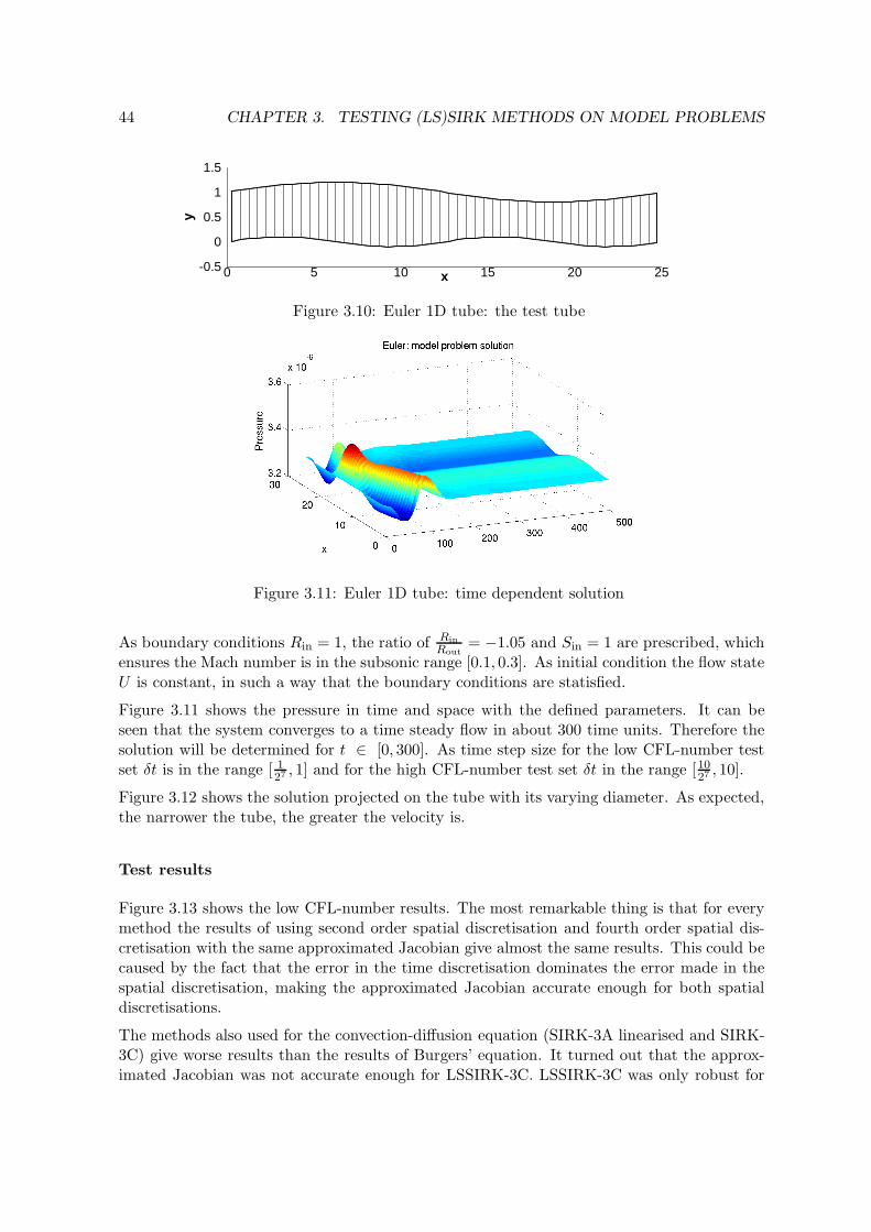
44 CHAPTER 3. TESTING (LS)SIRK METHODS ON MODEL PROBLEMS
x
y
0 5 10 15 20 25-0.5
0
0.5
1
1.5
Figure 3.10: Euler 1D tube: the test tube
Figure 3.11: Euler 1D tube: time dependent solution
As boundary conditions Rin = 1, the ratio of RinRout
= −1.05 and Sin = 1 are prescribed, whichensures the Mach number is in the subsonic range [0.1, 0.3]. As initial condition the flow stateU is constant, in such a way that the boundary conditions are statisfied.
Figure 3.11 shows the pressure in time and space with the defined parameters. It can beseen that the system converges to a time steady flow in about 300 time units. Therefore thesolution will be determined for t ∈ [0, 300]. As time step size for the low CFL-number testset δt is in the range [ 1
27 , 1] and for the high CFL-number test set δt in the range [1027 , 10].
Figure 3.12 shows the solution projected on the tube with its varying diameter. As expected,the narrower the tube, the greater the velocity is.
Test results
Figure 3.13 shows the low CFL-number results. The most remarkable thing is that for everymethod the results of using second order spatial discretisation and fourth order spatial dis-cretisation with the same approximated Jacobian give almost the same results. This could becaused by the fact that the error in the time discretisation dominates the error made in thespatial discretisation, making the approximated Jacobian accurate enough for both spatialdiscretisations.
The methods also used for the convection-diffusion equation (SIRK-3A linearised and SIRK-3C) give worse results than the results of Burgers’ equation. It turned out that the approx-imated Jacobian was not accurate enough for LSSIRK-3C. LSSIRK-3C was only robust for

3.3. A SYSTEM OF NON-LINEAR EQUATIONS MODEL PROBLEM: THE EULER EQUATIONS45
x
y
0 5 10 15 20 25-0.5
0
0.5
1
1.5
velocity0.0320.0310.030.0290.0280.0270.0260.0250.0240.0230.0220.0210.02
Steady velocity in the tube
Figure 3.12: Euler 1D tube: steady solution
101
102
10−16
10−14
10−12
10−10
10−8
10−6
10−4
Time steps per time unit
Max
. abs
. err
or
Euler equations: low CFL−number
SIRK−3A (Newton: 2 steps) 2nd order spatialSIRK−3A (Newton: 3 steps) 2nd order spatialSIRK−3A (Newton: 4 steps) 2nd order spatialSIRK−3A (Newton: 5 steps) 2nd order spatialSIRK−3A (Linearised) 2nd order spatialSIRK−3C 2nd order spatialSIRK−3A (Newtop: 2 steps) 4th order spatialSIRK−3A (Newtop: 3 steps) 4th order spatialSIRK−3A (Newtop: 4 steps) 4th order spatialSIRK−3A (Newtop: 5 steps) 4th order spatialSIRK−3A (Linearised) 4th order spatialSIRK−3C 4th order spatialO(h)O(h2)O(h3)
Figure 3.13: Euler 1D tube: test results with low CFL-number
101
102
103
10−16
10−14
10−12
10−10
10−8
10−6
timesteps per time unit
max
. abs
. err
.
Euler 2nd order spatial low CFL with Newton and a tolerance ε = ε*(δt)3
epsilon* = 10−1
epsilon* = 10−2
epsilon* = 10−3
epsilon* = 10−4
O(h)O(h2)
O(h3)
Figure 3.14: Euler 1D tube: test results with low CFL and residual tolerance

46 CHAPTER 3. TESTING (LS)SIRK METHODS ON MODEL PROBLEMS
Number of steps per time unitTolerance ε∗ 1 2 4 8 16 32 64 128
10−01 1.106 1.717 2.104 2.375 2.593 2.816 2.931 2.97110−02 2.266 2.692 2.979 3.107 3.154 3.173 3.190 3.19210−03 3.668 3.773 3.787 3.759 3.732 3.708 3.712 3.71410−04 5.176 4.887 4.634 4.361 4.276 4.220 4.120 4.031
Table 3.1: Euler: avaraged number of Newton steps for low CFL numbers
0.1 110
−12
10−10
10−8
10−6
10−4
Time steps per time unit
Max
. abs
. err
or
Euler equations: high CFL−number
SIRK−3A (Newton: 2 steps) 2nd order spatialSIRK−3A (Newton: 2 steps) 4th order spatialSIRK−3A (Newton: 3 steps) 4th order spatialSIRK−3A (Newton: 4 steps) 4th order spatialSIRK−3A (Newton: 5 steps) 4th order spatialSIRK−3A (Newton: 6 steps) 4th order spatialSIRK−3A (Newton: 7 steps) 4th order spatialSIRK−3A (Newton: 8 steps) 4th order spatialSIRK−3A (Newton: 9 steps) 4th order spatialSIRK−3A (Newton: 10 steps) 4th order spatialO(h)O(h2)O(h3)
Figure 3.15: Euler 1D tube: test results with high CFL-number
very small time steps sizes, that is why it is missing in the plots. As expected SIRK-3A lin-earised and SIRK-3C only show first order convergence. SIRK-3A linearised gave nice resultsfor Burgers’ equations for larger time step sizes, which made it a potential preconditioner forusing as initial Newton step. Due to the results here, this is no longer considered as an option.Both methods also had problems with the largest time step size, so they are not tested forthe high CFL-numbers tests.
The Newton methods behave about the same for the Euler equations as for Burgers’ equationswith the approximated Jacobian. Two and three Newton steps give about first and secondorder convergence. More steps give third order convergence.
Also a test has been run with a variable number of Newton steps based on a tolerancestopping criterion ε∗ as described in equation (2.10), table 3.1 shows the number of Newtonsteps needed for the required tolerance. Figure 3.14 shows the results. As can be seen thefour different tolerances give all rise to a third order convergence, although using a smallertolerance gives smaller errors. Making the relative tolerance ε∗ ≤ 10−4 gives convergenceproblems, since ε = ε∗(δt)3 becomes very small, near machine precision, in that case. Whenε∗ = 10−4 is used the results are the same as SIRK-3A with five fixed Newton steps in 3.14,while here only (depending on the time step size) somewhere between four and five steps areneeded. In this testcase using a tolerance-based stopping-criterion prevents using too manyNewton steps in the “easier” time regions of the problem. Some remarks about the relationof number of Newton steps needed for the different time step sizes and tolerances are madeat the end of the results of the high CFL test case.
Figure 3.15 shows the results of the high CFL-number tests. Only the Newton methodconverged here. Except for two Newton steps, the results for second and fourth order spatial

3.3. A SYSTEM OF NON-LINEAR EQUATIONS MODEL PROBLEM: THE EULER EQUATIONS47
0.1 1 1010
−14
10−12
10−10
10−8
10−6
timesteps per time unit
max
. abs
. err
.Euler 2nd order spatial high CFL with Newton and a tolerance ε = ε*(δt)3
ε* = 10−2
ε* = 10−3
ε* = 10−4
ε* = 10−5
ε* = 10−6
O(h)O(h2)
O(h3)
Figure 3.16: Euler 1D tube: test results with high CFL and residual tolerance
Number of steps per time unitTolerance ε∗ 0.1 0.2 0.4 0.8 1.6 3.2 6.4 12.8
10−02 1.022 1.144 2.133 3.650 4.519 4.749 4.648 4.49210−03 2.122 3.544 5.969 7.181 7.178 6.588 5.985 5.45310−04 7.500 10.022 12.008 11.766 10.256 8.581 7.334 6.47210−05 16.366 20.361 20.175 17.073 13.504 10.687 8.732 7.49010−06 34.355 34.988 29.575 22.690 16.879 12.805 10.198 8.535
Table 3.2: Euler: avaraged number of Newton steps for high CFL numbers
discretisation were the same. To keep the figure tidy only the results of the fourth orderspatial discretisation are shown. To let the error behave like δt3 for the high CFL tests aboutnine Newton steps are needed, but the most important thing is that the method is robust forthe higher CFL numbers. Time accuracy for such high CFL-numbers is not expected. Thelines representing less Newton steps all seem to tend to the line representing nine Newtonsteps line when the CFL-number decreases, which is expected, since in figure 3.13 four Newtonsteps are already sufficient for third order convergence for CFL numbers in the same region.
Here also a test has been run with a variable number of Newton steps based on a tolerancestopping criterion as described in equation (2.10), table 3.2 shows the number of Newton stepsneeded for the required tolerance. Figure 3.16 shows the results. Using ε∗ ≤ 10−4 gives thesame error, indication that that is the maximum precision of the SIRK-3A method. Thoseresults are third order. Using a greater tolerance ε∗ shows that SIRK-3A is still robust forhigh CFL numbers. Also here for the most accurate results on avarage less Newton steps areneeded then when a fixed number of Newton steps is used.
The number of Newton steps Nn needed to obtain the required tolerance ε∗ seems to increasefirst when the number of time steps per time unit Nt is growing. But after a certain Nt, Nn
decreases again. The point where Nn starts to decrease seems to become smaller as ε∗ does.The reason why the number of Newton steps Nn first increases when Nt is growing, is thatthe relative tolerance ε∗ decreases with δt3. Because at a certain point δt is decreasing, thedifference between two time steps becomes so small, that again the number of Newton stepsNn needed to obtain the required tolerance is decreasing.

48 CHAPTER 3. TESTING (LS)SIRK METHODS ON MODEL PROBLEMS
3.4 Discussion
3.4.1 (LS)SIRK-3C
SIRK-3C and its low storage variant LSSIRK-3C are derived in such a way that when theexact Jacobian is used, only linearising the residual while treating the implicit term is neededto obtain (theoretically) third order results. LSSIRK-3C is theoretically the preferred method,because it is low storage and only one Jacobian inversion is needed each Runge-Kutta stage.
As expected the error of LSSIRK-3C was greater than the error of SIRK-3C, since LSSIRK-3C is low storage. When the exact Jacobian was used, the error was third error, only theerror constant was a lot larger than with for example SIRK-3C. When the Jacobian wasapproximated, the results were only first order and not robust at all. Since using the exactJacobian in ENSOLV is presumably too expensive and the error is a lot worse than the othermethods, LSSIRK-3C is not useful for ENSOLV.
SIRK-3C performed well for linear problems and when the exact Jacobian was used. SinceSIRK-3C only needs one Jacobian inversion for solving the implicit term, it is a lot cheaperthan SIRK-3A with the Newton method. But when the Jacobian was approximated theresults became worse, which makes SIRK-3A unusable for ENSOLV in the current situation.
3.4.2 SIRK-3A without the Newton method
Using SIRK-3A with the implicit term solved with MATLAB’s algorithm is undoubtfully themost robust method to use, but it is terribly slow comparing to the other methods due to thealgorithm MATLAB uses to find the solution. Using this method is useless for solving verylarge systems, but it was useful for comparing the various SIRK-3A based methods.
SIRK-3A with the implicit term linearised only performed well with linear problems, whichmakes sense. With Burgers’ equation it outperformed SIRK-3C for large timesteps, whichmade it a potential candidate as a preconditioner for Newton, but the results of the Eulermethod for larger time steps were not robust. Overall SIRK-3C performed better than SIRK-3A with the implicit term linearised and SIRK-3C was already not good enough, so SIRK-3Awith the implicit term linearised is also not good enough.
3.4.3 SIRK-3A with the Newton method
Although SIRK-3A with the implicit term solved by the Newton method is a bit slower thanmost other methods, it is robust for Burgers and Euler (even with high CFL numbers) andshows third order convergence. When an approximated Jacobian instead of the exact Jacobianis used in the Newton process, more Newton steps are needed to get third order convergence.
In practice using a fixed number of Newton iterations may be inefficient, since it is very prob-lem dependent how many iterations are needed. Using a tolerance-based stopping-criterionhas many advantages, first when there is a difficult part in the solution more iterations areused and when there is a more steady part it can use less Newton iterations.

3.4. DISCUSSION 49
3.4.4 Final choice
Since robustness is as important as the performance SIRK-3A with the Newton method basedon an approximated Jacobian will be used, which has a decent robustness and is fast. UsingSIRK-3A with the implicit term solved exactly or solving the Jacobian exactly with SIRK-3Cis much too expensive. As stopping criterion a relative tolerance limited by a fixed number ofNewton steps will be used. Presumably about five Newton steps are needed per Runge Kuttastage. Combining this with the formulaes and testcases from 2.3 leads this to an expectedperformance increase of γimp ≈ 26 for the full implicit case with the same grid size. Whenthe performance of the coupling test case is considered an increase of γcoup ≈ 14 is expected.

50 CHAPTER 3. TESTING (LS)SIRK METHODS ON MODEL PROBLEMS

Chapter 4
Implementation
In ENSOLV the flow domain is divided in separate non-overlapping blocks. Each blockhas the topology of a square and is bounded by six faces, with a whole range of possibleboundary conditions for each face. In each block different types of flow equations can besolved, for example the RANS equations with different types of turbulence modelling and theEuler equations. For the unsteady time discretisation different options are available, whichcan differ from block to block, as long as they have a method implemented to exchangeinformation at the connecting boundary faces. In practice, blocks with a coarse grid anda low aspect ratio (far away from surfaces) will be treated explicitly and the blocks with afiner grid and a high aspect ratio (near a surface) will be treated with some form of implicitmethod. More information about the different flow solver options for ENSOLV can be foundin reference [5].
As can be found in the discussion sections of the previous sections, SIRK-3A was the bestoption for ENSOLV. The implicit term will be treated with the Newton method, which usesthe Jacobian already implemented in ENSOLV. In the blocks near a surface the full semi-implicit SIRK-3A can be used, while in the explicit areas only the explicit part of the SIRK-3Ascheme can be used. This avoids many coupling problems, since at each Runge-Kutta stagethe information of the connected blocks is available and can be exchanged. The last grid cellface on the boundary of a semi-implicit block connecting to an explicit block will be treatedexplicitly. The last property is implemented in ENSOLV, while it is not considered in theprevious testcases. Since it is likely that the grid cells connecting to an explicit block do nothave a high aspect ratio, no restrictions in terms of the CFL number will be introduced bythis. The final tests can tell whether this is a problem for the convergence order of the timeintegration method or not.
The low storage Runge-Kutta scheme already implemented in ENSOLV resembles the SIRK-3A scheme that is implemented now. It has already the means implemented to exchange theflow information at the boundary of two connecting blocks each Runge-Kutta stage. Thismethod will be used as a basis for the implementation of the SIRK-3A scheme.
To omit bugs in the implementation, the implementation itself is done in two phases. Sincethere is no non low-storage Runge-Kutta scheme available in ENSOLV, this is implementedand tested first. During this implementation the classical Runge-Kutta 4 scheme is used fortime integration method.
51

52 CHAPTER 4. IMPLEMENTATION
Secondly, the semi-implicit part is implemented. This yields the implementation of the New-ton method and adjusting the residual and boundary condition functions in such a way thatthe spatial directions can be treated separatly. Almost all residual and boundary conditionfunctions are already implemented in such a way that this is fairly easy to do. A problem oc-curs with the turbulence models: the production and dissipation terms which are introducedby those models have to be split. Unfortunaly there was no time left during this project forresearching the details of splitting the turbulence terms and its implementation.
More details about the implementation, the new input parameters, the memory managementand the modified and newly introduced functions are explained in appendix A.

Chapter 5
ENSOLV test results
In this section two test cases will be considered extensively: the already known test case withthe one dimensional Euler tube, from section 3.3.4, and the flow around a laminar cylinderwith a Reynolds number of 500. During the implementation also a few very simple test caseswere used. These are considered briefly in the first section of this chapter.
5.1 Small tests during the implementation
The tests that were run during the first and second phase of the implementation all used thesame two grids. The first one was a uniform cubic grid with sixteen grid cells in each directionused for normal CFL numbers. The second grid is a rectangular one which has a high aspectratio, for use with high CFL numbers. It has sixteen grid cells in each direction, only oneside of the rectangle is a hunderd times smaller than the other two sides. For the tests, allboundary conditions were set to ’general free-stream’ to obtain a uniform flow. At default,ENSOLV uses the correct uniform flow as initial condition and the first grid was used.
The goal of the first test was to see whether this uniform flow was maintained after the firstphase of the implementation. This test was performed first with the Euler equations and assoon as the correct solution was obtained, it was also tested with RANS and TLNS.
When the first tests succeeded, the same tests were run with a disturbance in the initialcondition. The goal of these is to see whether the uniform flow is obtained after a disturbance.The disturbance was created by starting the test using a different angle of attack of the flowand then restarting using an angle of attack of zero.
To finish the validation of the first phase of the implementation a convergence test was run.A standard test case from ENSOLV was used: the flow around an oscillating NACA0012profile. The results using the coefficients of the classical Runge-Kutta 4 method were fourthorder in time and the results using the explicit coefficients of SIRK-3A were third order intime, as expected.
During the second phase of the implementation the tests to maintain and obtain a uniformflow were used again. Now the test cases were run on both the first and second grid. On thefirst grid all test were run three times, using each direction as implicit direction once. On thesecond grid the implicit direction was of course the direction with the finest grid cells. Whenthe expected solutions were obtained, the tests described in the next sections were considered.
53

54 CHAPTER 5. ENSOLV TEST RESULTS
x0
510
1520
25
Time0 10 20 30 40 50 60
No
rm. p
ressure
0.96
0.98
1
1.02
1.04
1.06
Y
Z
X
ENSOLV Solution
Figure 5.1: New Euler 1D Tube: results with ENSOLV with CFL = 2
5.2 1D Euler tube revisited
This test case is considered to compare the results from section 3.3.4, further refered toas the MATLAB results, with results produced by ENSOLV. There are two big differencesfrom the implementation in MATLAB and the implementation default in ENSOLV. The firstone is the parameter used for making the equations dimensionless and the second one isthe implementation of the Riemann in- and outflow boundary conditions. To solve the firstproblem, the implementation in MATLAB is made dimensionless with the same parametersas ENSOLV, that is the tempature T∞, the pressure p∞ and the density ρ∞.
The difference between ENSOLV and the implementation in MATLAB in the Riemann in-and outstream boundary conditions can be found in the way the enthalpy is treated. InENSOLV the enthalpy is treated separately, in order to make the constant enthalpy an exactsolution of the discrete equations in case of inviscid flow. To make the behaviour of MATLABand ENSOLV the same, the enthalpy is not treated separately for this test in ENSOLV.
Exactly the same input parameters are used for the test, that is a Mach number M∞ = 0.2and γ = 1.4. The solutions of MATLAB and ENSOLV are almost the same for different timestep sizes (with high and low CFL numbers). The relative error between both solutions isabout 10−8 with the absolute value of the solution in the order of one. This error is probablycaused by the fact that the grid points were treated with single precision instead of doubleprecision somewhere in the process of converting the grid from MATLAB to ENSOLV.
Figure 5.1 and 5.2 show an example of the solutions from ENSOLV and MATLAB withδt = 0.1, resulting in a CFL number of 2. Figure 5.3 shows an example with a greater CFLnumber and δt = 1.0. It can be seen that the time step is too coarse to obtain a time accuratesolution in the first part of the solution, but it convergences to the same steady solution aswith a lower CFL number.
Figure 5.4 shows the results of the convergence test run with both the MATLAB and the

5.2. 1D EULER TUBE REVISITED 55
x0
510
1520
25
Time0 10 20 30 40 50 60
No
rm. p
ressure
0.96
0.98
1
1.02
1.04
1.06
Y
Z
X
MATLAB Solution
Figure 5.2: New Euler 1D Tube: results with MATLAB with CFL = 2x
0
5
10
15
20
25
Time0 5 10 15 20
Norm
. pressure
0.97
0.98
0.99
1
1.01
1.02
XY
Z
ENSOLV high CFL number
Figure 5.3: New Euler 1D Tube: results with ENSOLV with CFL = 20
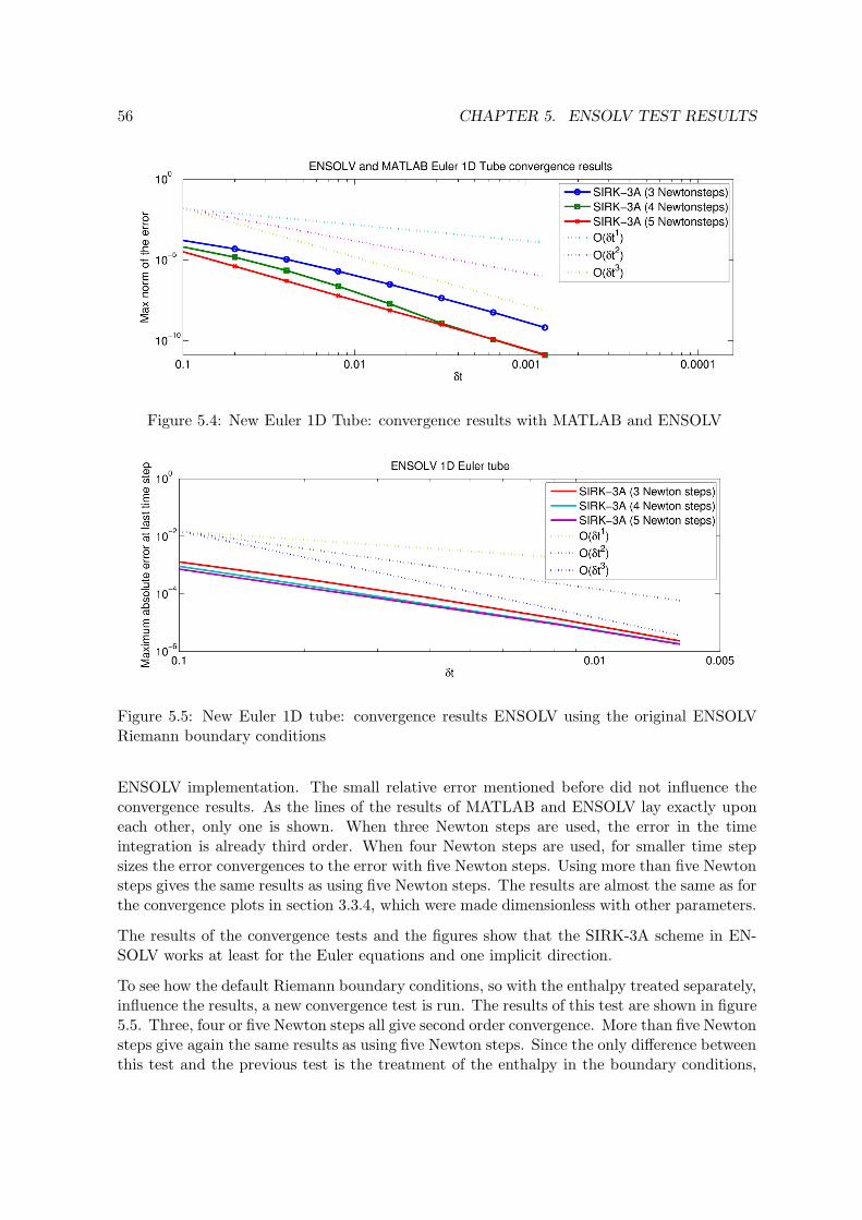
56 CHAPTER 5. ENSOLV TEST RESULTS
Figure 5.4: New Euler 1D Tube: convergence results with MATLAB and ENSOLV
Figure 5.5: New Euler 1D tube: convergence results ENSOLV using the original ENSOLVRiemann boundary conditions
ENSOLV implementation. The small relative error mentioned before did not influence theconvergence results. As the lines of the results of MATLAB and ENSOLV lay exactly uponeach other, only one is shown. When three Newton steps are used, the error in the timeintegration is already third order. When four Newton steps are used, for smaller time stepsizes the error convergences to the error with five Newton steps. Using more than five Newtonsteps gives the same results as using five Newton steps. The results are almost the same as forthe convergence plots in section 3.3.4, which were made dimensionless with other parameters.
The results of the convergence tests and the figures show that the SIRK-3A scheme in EN-SOLV works at least for the Euler equations and one implicit direction.
To see how the default Riemann boundary conditions, so with the enthalpy treated separately,influence the results, a new convergence test is run. The results of this test are shown in figure5.5. Three, four or five Newton steps all give second order convergence. More than five Newtonsteps give again the same results as using five Newton steps. Since the only difference betweenthis test and the previous test is the treatment of the enthalpy in the boundary conditions,

5.3. FINAL TEST CASE: LAMINAR CYLINDER AT RE=500 AND M∞ = 0.3 57
so an explanation of the fact that these results are only second order should be found inthe boundary conditions. The loss of an order in the convergence rate also occurs when anon-autonomous differential equation is used with a three stage SIRK scheme. In reference[10] it is stated that when a non-autonomous differential equation is considered, a four stageSIRK scheme is needed to get third order results. However, threating the enthalpy seperatelyin the boundary conditions does not make the differential equations non-autonomous.
5.3 Final test case: Laminar cylinder at Re=500 and M∞ = 0.3
5.3.1 Problem definition
As final test case a laminar flow around a cylinder is computed. The main purpose of thistest is to see how SIRK-3A performs with a test case, which is comparable with a realapplication. To avoid turbulence a Reynolds number of 500 is chosen, to avoid shocks a theMach number M∞ of 0.3 is chosen. At the in- and outflow boundaries Riemann invariantboundary conditions are used.
A finer grid than necessary is used for this problem; the grid used was intented to performa full X-LES simulation. Using this grid, a better comparison in performance of SIRK-3Aand the B3 method with pseudo time steps, now usually used in ENSOLV, can be made.Figure 5.6 shows the grid. The three blocks around the cylinder are computed semi-implicitlyand the three outer blocks are computed explicitly. The semi-implicit blocks have a total of7680 grid cells and the explicit blocks have a total of 20480 grid cells. The grid cell with thebiggest aspect ratio lies in the block left of the cylinder. The measurements of that grid cell
are δxnormal = 0.00023 and δxtangential = 0.018, which gives an aspect ratio ofδxtangential
δxnormal≈ 80.
The builtin CFL condition checker of ENSOLV is used to determine the minimal time step size.As can be found in section 2.1.2, SIRK-3A is stable for CFLexplicit ≤ 1.5. The correspondingtime step size is δt = 0.00375. Knowing this and the aspect ratio, it follows that CFLimplicit ≈80×1.5 = 120. The number of grid cells in the boundary layer will be sufficient since the gridis much finer than needed for this problem. The actual number of grid cells in the boundarylayer will be determined in the tests.
Three tests will be considered. The first is to obtain a Von Karman street behind the cylinder.The last point of this simulation will be used as the initial condition for the other tests. Thesecond test will be a convergence test. The third test will be a comparison in computationtime when a fixed period is solved with B3 with pseudo timestepping or SIRK-3A.
5.3.2 Test 1: Obtaining a Von Karman street with SIRK-3A
Since the grid is symmetric, a little disturbance in the initial condition was needed to geta vortex shedding street. Using the normal initial condition, which is also symmetric, willconverge to a time steady solution which is symmetric. The disturbance was created bystarting the test with a small angle of attack and then restarting with an angle of attackequal to zero.
Figure 5.7 shows the lift and drag coefficient from the restart with the angle of attack equalto zero up to the restart point for the further tests. It converges to a period solution as was

58 CHAPTER 5. ENSOLV TEST RESULTS
X
Y
Z
Grid around cylinder
SIRK-3A semi-implicit
SIRK-3A explicitSIRK-3A explicitSIRK-3A explicit
X
Y
Z
Full grid
X
Y
Z
Grid near surface
Figure 5.6: Laminar cylinder: grid

5.3. FINAL TEST CASE: LAMINAR CYLINDER AT RE=500 AND M∞ = 0.3 59
number of physical time stepstota
ldra
gco
effic
ient
,tot
alsi
de-f
orce
coef
ficie
nt
5000 10000 15000 20000-2
-1.5
-1
-0.5
0
0.5
1
1.5
2
2.5
total drag coefficienttotal lift coefficient
Figure 5.7: Laminar cylinder: the lift and drag coefficient up to the restart point
Figure 5.8: Laminar cylinder: the vortex street at the restart point

60 CHAPTER 5. ENSOLV TEST RESULTS
Figure 5.9: Laminar cylinder: convergence results ENSOLV
Number of Newton steps
δt 2 6 8 10 20
0.003 0.19167 0.67657 0.74344 0.82697 0.831830.0015 0.39593 0.91338 0.89593 0.87027 0.910690.00075 0.64061 0.95711 1.0410 1.1039 1.08110.000375 0.79751 1.0902 1.0563 1.0262 1.07050.0001875 0.94401 1.1263 1.1929 1.2551 1.31590.00009375 1.0271 1.3951 1.5160 1.6405 1.76810.000046875 1.1008 1.8849 2.0378 2.1185 2.1989
Table 5.1: Laminar cylinder: convergence results ENSOLV using a different approach
expected. The length of a period is 4.2, which is the same length as was obtained with a B3with pseudo time stepping run. Figure 5.8 shows the Von Karman street which was formedbehind the cylinder. Using this solution the number of grid cells normal to the surface in theboundary layer is determined. There were 36 grid cells in the boundary layer. The final timestep of this will be called the restart point for the next two tests.
5.3.3 Test 2: Convergence results after restart
The convergence tests started at the restart point. Since the grid was very large and thetimesteps already very small, it was not possible to create a very accurate reference solutionfor figure 5.9. Where in the previous figures a solution with a time step eight to sixteentimes smaller than the smallest considered error was used, now the reference solution had atime step size of just two times smaller that the smallest considered error. Since this mightinfluence the convergence rate also another method was used. The solution U can be writtenas: Uδt = Uexact + Cδtp, with p the order of convergence and C a constant. When
2 log
∥∥∥Uδt − U 12δt
∥∥∥∞∥∥∥U 1
2δt − U 1
4δt
∥∥∥∞
=2 log
( ∥∥C(((δt)p −
(12δt)p)∥∥
∞∥∥C((
12δt)p −
(14δt)p)∥∥
∞
)
= p

5.3. FINAL TEST CASE: LAMINAR CYLINDER AT RE=500 AND M∞ = 0.3 61
is considered, the order of convergence is easily found. The results can be found in table 5.1.
As said before, figure 5.9 and table 5.1 show the results. From 8 Newton steps on the resultstend to be second order convergence in time. Using more then 20 Newton steps gives thesame results as using 20 Newton steps. Perhaps the, already very small, smallest time stepsize is not yet in the convergence area of the method. When the results are in table 5.1extrapolated to even smaller timesteps, the convergence seems to get better than secondorder. Two possible explanations for this result are given. The first one are the Riemanninvariant boundary conditions, which also where a problem with the Euler tube test case.The second one could be the coupling between the semi-implicit and explicit blocks. Moreresearch is needed to see how treating the last face in the implicit direction in a semi-implicitblock influences the convergence order of the SIRK-3A scheme.
Comparing this to results of high CFL tests found in 3.3.4, the results from this test showthe same behaviour. For high CFL numbers more Newton steps are needed to get the properconvergence order.
5.3.4 Test 3: Comparing to B3 method with the pseudo time stepping
From the restart point, 3.75 physical time units extra are computed, which is a little lessthan one period. This is done because after exact a period, the solution is the same as therestart solution. First a test is run with the full implicit B3 method, the second and thirdwith SIRK-3A with respectively 5 and 8 Newton steps.
In order to get a good comparison of the computation time between SIRK-3A and B3, it isnecessary to use the time step sizes that would be used when a X-LES simulation was run.The time step restriction of SIRK-3A is based on the CFL number based on the maximumwave speed,
CFLSIRK-3A =(|u| + c)δtSIRK-3A
δx,
where c is the speed of sound. An estimation for the maximum wave speed is made, |u|+ c ≈U∞+a∞ = U∞
(1 + 1
M∞
), where U∞ is the free stream velocity. Since B3 is fully implicit, no
real numerical CFL restriction exists. For accuracy considerations the time step restrictionused for the B3 scheme is based on the flow velocity,
CFLB3 =U∞δtB3
δx.
If the same maximum value for the CFL number is used, a realistic time step for the B3method will be
δtB3 = (1 +1
M∞
)δtSIRK-3A.
Recalling from 5.3.1 that M∞ = 0.3 and δtSIRK-3A = 0.00375 gives δtB3 = 0.01625. Toobtain an integer value of time steps, δtB3 = 0.015 is used.
Figures 5.10 to 5.12 show the solutions after 3.75 physical time from the restart point. SinceB3 and SIRK-3A are totally different time-integration methods it cannot be assumed that thesolutions are exactly the same here. This could only be assumed for very small time step sizes.As can be seen in these figures the differences between the solutions are small. To compareboth solutions the maximum difference over all grid cells, normalized by the maximum value

62 CHAPTER 5. ENSOLV TEST RESULTS
X
Y
ZTotal pressure loss
0.180.160.140.120.10.080.060.040.020
-0.02-0.04-0.06-0.08
ENSOLV Laminar cylinder, measure point with pseudo timeste pping
Figure 5.10: Laminar cylinder: the final point with B3 and 30 pseudo time steps
X
Y
ZTotal pressure loss
0.180.160.140.120.10.080.060.040.020
-0.02-0.04-0.06-0.08
ENSOLV Laminar cylinder, measure point with SIRK-3A (5 Newt on steps)
Figure 5.11: Laminar cylinder: the final point after the restart with SIRK-3A and 5 Newtonsteps

5.3. FINAL TEST CASE: LAMINAR CYLINDER AT RE=500 AND M∞ = 0.3 63
X
Y
ZTotal pressure loss
0.180.160.140.120.10.080.060.040.020
-0.02-0.04-0.06-0.08
ENSOLV Laminar cylinder, measure point with SIRK-3A (8 Newt on steps)
Figure 5.12: Laminar cylinder: the final point after the restart with SIRK-3A and 8 Newtonsteps
Method CPU Time (in minutes)
B3 with thirty pseudo timesteps (δt = 0.015) 210SIRK-3A with five Newton steps (δt = 0.00375) 24SIRK-3A with eight Newton steps (δt = 0.00375) 30
Table 5.2: Laminar cylinder: Computation time results. The tests were performed on a IntelCore2-Duo based workstation.
in the flow domain, is considered. For the total pressure loss between SIRK-3A with 5 Newtonsteps and B3 the difference is about 2 procent and the difference between SIRK-3A with 8Newton steps and B3 is about 1.5 procent.
The most interesting part of this test are the CPU times that were necessary to get the results.In this test case SIRK-3A with five Newton steps is about nine times faster than B3, witheight Newton steps it is about seven times faster. As said before, the grid is representativefor X-LES, but there are other things which influence the performance increase of SIRK-3Aon B3. The ratio in time step size between both methods depends on the Mach number:1 + 1
M∞
. This ratio for M∞ = 0.3 is 4.33, but for example forM∞ = 0.8 it is 2.25 and forM∞ = 0.1 it is 0.1. Also using a higher aspect ratio in the grid creates extra performanceincreases for SIRK-3A. Knowing this it can be safely said that SIRK-3A is in practice at leastseven times faster than B3 using M∞ ≥ 0.3. When M∞ = 0.8 is used, SIRK-3A is about 14times faster. This the same result as the estimation γcoup = 14, which was made in section3.4. Also the dispersion and dissipation is better than B3 and the smaller time step sizeneeded for SIRK-3A gives a smaller error. So SIRK-3A gives a more accurate answer for lesscomputation time than B3.

64 CHAPTER 5. ENSOLV TEST RESULTS

Chapter 6
Concluding remarks
The extra-large eddy simulations model, a combination of the Reynolds-averaged Navier-Stokes (RANS) equations and large eddy simulations (LES), has been used to simulate time-dependent flow around aerospace vehicles. X-LES increases details of the flow physics overRANS, without the cost of a full LES or DNS (Direct Navier Stokes) simulation. Calculatingdynamic flows cost a lot of computational time, therefore an efficient time integration hasbeen developed. A semi implicit Runge-Kutta (SIRK) scheme can be used to calculate theflow very efficiently, using an explicit time integration in the LES area and a semi-implicittime integration in the RANS area. Semi-implicit time integration consists of an implicittime integration for the stiff spatial direction (normal to a surface) and an explicit timeintegration for the other spatial directions. Different flavours of SIRK schemes have beentested in this report. SIRK-3A with a Newton method to calculate the implicit term was themost applicable for use with the X-LES method in ENSOLV. As stated in the introduction,SIRK-3A had to meet the following requirements:
1. The dissipation and dispersion have to be comparable to the time integration methodsnow used (B3 for the implicit part and Runge-Kutta 4 for the explicit part),
2. The method needs to be at least second order accurate in time,
3. The approximated Jacobian used in the current line-implicit scheme should also workas Jacobian for the SIRK methods,
4. The implicit solver has to be an order faster than the method with pseudo timesteps,now used for X-LES.
All those requirements were treated extensively in this report. The results of the first re-quirement can be found in section 2.1.7. In the RANS areas the dissipation and dispersionof SIRK-3A was much better than the dissipation and dispersion from B3. In the LES areasthe dissipation and dispersion of SIRK-3A were close to the dissipation and dispersion ofRunge-Kutta 4. So the first requirement is met.
The second requirement is about the accuracy in time. For autonomous problems SIRK-3Ais third order, see section 2.1.1. For the model problems the results were also third orderwhen sufficient Newton steps were used. In the ENSOLV test cases (see chapter 5) it turned
65

66 CHAPTER 6. CONCLUDING REMARKS
out that using Riemann invariant boundary conditions resulted in second order convergenceinstead of third order convergence. Second order convergence still meets the requirements.
The third requirement is tested in the model problems by the 1D Euler tube test case (seesection 3.3) and of course with the ENSOLV testcases. Using the approximated Jacobian asJacobian with SIRK-3A using the Newton method for the Jacobian did not give any problemsin terms of convergence or robustness. The other SIRK flavours gave worse results when theapproximated Jacobian was used. This had been the main reason why SIRK-3A is the mostapplicable. So SIRK-3A also meets this requirement.
The last requirement has been tested in the last test case from chapter 5. A lot of parametersinfluence the difference in computation time for the B3 method and SIRK-3A. This test caseused a representative grid but the other conditions where in favour to B3. Nevertheless SIRK-3A was seven times faster than B3. When a higher Mach number or a grid with a higheraspect ratio had been used, the performance increase would be about fourteen times. This isthe same result that was predicted during the model problems. So the last requirement hasbeen also fulfilled.
Since all requirements are met, SIRK-3A with a Newton method for the implicit term hasbeen succesfully implemented and tested in ENSOLV. Unfortunately only RANS, TLNS andEuler equations were adjusted for use with SIRK-3A. The handling of the turbulence models,needed by X-LES, for use with SIRK-3A were not implemented yet due to a lack of time.
For future work, the following may be considered:
• The turbulence models have to be adjusted for use with SIRK-3A
• The coupling between the explicit LES blocks and the semi-implicit RANS blocks. Nowthe last face on the boundary between two connecting blocks in the normal directionis treated explicitly in stead of implicitly. Further research is needed to see how thisinfluences the order of convergence of the SIRK method and the conservativity of thespatial discretisation.
• In this report it was assumed that X-LES was autonomous, therefore only three stageSIRK schemes were considered. Those schemes were third order of convergence, as-suming that the problems were autonomous. In reference [11] and reference [10] alsofour stage SIRK schemes are proposed, which have a third order of convergence fornon-autonomous problems. These schemes could also be considered for X-LES, espe-cially with Riemann invariant boundary conditions which showed only second orderconvergence.
Aknowledgements
This work would not be the same without the support of a number of people.
I would would like to thank the National Aerospace Laboratory (NLR) to facilitate me withthe internship which resulted in this report, especially the manager of the division FlightPhysics and Loads: ir. Koen de Cock.
Furthermore, I would like to thank my direct supervisors dr. Johan Kok and dr. Harmen vande Ven for their enormous input during my research and while writing this report. I would

67
also like to thank prof. dr. Arthur Veldman for introducing me in the domain of CFD and forhis valuable comments while I was writing this report. I also would like to thank my fellowinternship colleague, Pim Hooghiemstra, for the pleasant time we had during our internships.

68 CHAPTER 6. CONCLUDING REMARKS

Bibliography
[1] R. L. Burden and J. D. Faires. Numerical Analysis. Brooks/Cole, seventh edition, 2001.
[2] J. C. Kok. An Industrially Applicable Solver for Compressible Turbulent Flows. PhDthesis, TU Delft, 1998.
[3] J. C. Kok. Numerical design of ensolv version 3.20 a flow solver for 3d euler/navier-stokesequations in arbitrary multi-block domains. Technical report, NLR-CR-2000-620, 2000.
[4] J. C. Kok. A computational aeroacoustic method for aircraft noise propagation. Technicalreport, NLR-CR-2003-629, 2003.
[5] J. C. Kok and B. B. Prananta. User guide of ENSOLV version 6.32.
[6] J. C. Kok and B. I. Soemarwoto. Time-accurate computational fluid dynamics algorithmfor unsteady aerodynamic load applications. Technical report, NLR-CR-2003-635, 2003.
[7] M. Scheijbeler. An efficient time integration method for extra-large eddy simulations.Master’s thesis, RuG, 2005.
[8] A. E. P. Veldman. Computational fluid dynamics. RuG lecture notes, 2004.
[9] F. Wubs. Computational methods of science. RuG lecture notes, 2004.
[10] K. Yoh and X. Zhong. Low-storage semi-implicit Runge-Kutta methods for reactive flowcomputations. AIAA, Aerospace Sciences Meeting & Exhibit, 36 th, Reno, NV, 1998.
[11] X. Zhong. Additive Semi-Implicit Runge-Kutta Methods for Computing High-SpeedNonequilibrium Reactive Flows. Journal of Computational Physics, 128(1):19–31, 1996.
69

70 BIBLIOGRAPHY

Appendix A
Software Design
This part of the report contains the changes that have to be made for implementing a nonlow storage semi-implicit Runge-Kutta scheme with the implicit term solved by the Newtonmethod into ENSOLV.
A.1 New variables and input parameters
A.1.1 New input parameters
The following new parameters are added to the input file IN:
RKLS: Indicator whether to use low storage Runge-Kutta (0=normal RK, 1=low-storage RK)
SIRK: Indicator to use a SIRK-rA with a Newton implicit term solver (ImpliesRKLS = 1)
NWTNTO: Stop the implicit Newton solver when a certain relative tolerance is obtained
NWTNST: Maximum number of Newton steps per stage.
COEFAnn: Coefficients for the explicit intermediate flow states for Runge-Kutta
COEFBnn: Coefficients for the implicit intermediate flow states for Runge-Kutta
COEFn: (changed) The Runge-Kutta coefficients for the final flow state.
When normal Runge-Kutta is selected, by default NSTAGE, COEFn and COEFAnn will be setas Runge-Kutta 4. In mathematical using the parameters NSTAGE,COEFn and COEFAnn theRunge-Kutta scheme looks like:
u1 = u0 −NSTAGE∑
i
COEFj ki
ki = δt
f(u0 +
i−1∑
j
COEFAij kj) + g(u0 +
i∑
j
COEFBij kj)
,
71

72 APPENDIX A. SOFTWARE DESIGN
where f and g respectively are the nonstiff (explicit) and stiff (implicit) part of u′ + f(u) +g(u) = 0 .
A.1.2 New variables
ENSOLV uses one long workspace array to store all grid-dependent data. Each separatevariable is located in the workspace array by a pointer and by its length. New variables areadded to the workspace by the following pointer and length parameters:
pdvrk(b,s) Pointer to flow state differences at sth Runge Kutta stage of the bth block.
ldvrk(b,s) Length of flow state differences at sth Runge Kutta stage of the bth block.
pdvimp Pointer to temporary flow state differences during implicit calculations
ldvimp Length to temporary flow state differences during implicit calculations
The parameters will be initialised the same way as the parameters for the initial flow state.
As in the previous section the Newton method is shown below, to make clear what variableis used for what part of the computation. In section 2.2.3 a short derivation of the methodcan be found, here the results are recalled. To compute a Runge-Kutta stage ki the followingcomputations are required:
k(l)i = k
(l−1)i − K−1(k
(l−1)i )H(k
(l−1)i ),
where
H(ki) = ki − δt(f(un +
i−1∑
j=1
bijkj) + g(un +
i−1∑
j=1
cijkj + diki)) and
K = I − δtdiJ(un +i−1∑
j=1
cijkj + dix).
This process is repeated until a certain tolerance based on k(l)i −k
(l−1)i = K−1(k
(l−1)i )H(k
(l−1)i )
is obtained. As can be seen, the explicit residual f stays unchanged each Newton step. It onlyhas to be calculated once and then it is stored in the existing variable DV. Each Newton stepthe implicit residue g has to be calculated. For this computation different flow state variablesare needed. These will be computed and stored in VRB. The implicit residue will be stored inthe new variable DVIMP. Now the explicit and implicit residues have to be combined to obtain
H(ki) and the results will overwrite DVIMP. To obtain K−1H from H(k(l−1)i ), almost the same
functions as the original line-implicit algorithm can be used. To compute the Jacobians, thesefunctions require the same implicit flow state variables as used for the computation of g, whichare still stored in VRB. Again the results will be stored in DVIMP. All the results needed the
compute k(l)i are gathered now and k
(l)i will be stored in the new variable DVRK(m). Since
K−1H is still in DVIMP, DVIMP can be used now to check whether the tolerance is obtainedyet.

A.2. THE IMPLICIT AND EXPLICIT PART OF THE RESIDUE 73
A.2 The implicit and explicit part of the residue
For the SIRK method it is necessary to be able to compute the residue in only one directionfor the implicit part (denoted by g in this report) and to compute the residue in the otherdirections for the other part (denoted by f). Currently in RESID, the function that computesthe residue, all directions are already treated separately in the underlying functions. For thecomputation of the boundary conditions a similar construction is used. To be able to computethe residue (and the corresponding boundary conditions) in only some of the directions thebooleans DOI, DOJ and DOK are introduced in the subroutine RKSTGB, which performs oneRunge-Kutta stage. The booleans indicate whether the residue should be determined in thei,j and/or k direction.
The changes that have to be made to the underlying functions of RESID are relatively small,but there are a lot of functions. To keep this report tidy, only the changes made to theEuler functions (EULER) are presented. The same changes are made for the artificial diffusionfunctions (FILTER), the RANS functions (RANS) and TLNS functions (TLNS). EULER is calledfrom RESID to compute the convective terms of the residue. A simplified version of thatfunction with changes is presented in the next section.
A.3 Changed functions

74 APPENDIX A. SOFTWARE DESIGN
Algorithm A.1 RELAX (Relaxation at level l)
One relaxation, on a certain grid level l of the FAS scheme consists of applying a relaxationstep for each block succesively. A relaxation for one block consists of taking one pseudo-timestep by a Runge–Kutta (RK) scheme.
in: l, XYZ, BCDinout: VAR, VARJK, SRFtemp: WS, IWS
for B = 1 to NB (parallellized loop over blocks) doif RANS equations ∨ (B is turbulent ∧ l = lFMG) thenBCINT = 1 (apply internal boundary conditions)call BCONDT (update dummy-cell values at faces of block B)
end ifend for Bif RANS equations then call XTEDGE (set dummy-cell values at edges)if turbulent ∧ l = lFMG then call TURALL (calculate eddy viscosity for all blocks)if block loop outside RK-stage loop then
for B = 1 to NB (parallellized loop over blocks) docall RELAXB (relax block B)
end for Bif Jacobi then
for B = 1 to NB (parallellized loop over blocks) docall COPVAR (copy intermediate flow states to permanent flow states)
end forend ifcall EXCVAR (exchange flow variables between domains at level l)
end ifif block loop inside RK-stage loop then
call RKL (Go into the RK-stage loop)end ifif l = lFMG ∧ selected iteration then
call BCALL (compute surface forces and force coefficients; update dummy-cells of allblocks)if selected iteration then call WRCONV (write convergence data to CONV )if selected iteration then call XTEDGE (set dummy-cell values at edges and vertices)if selected iteration then
if turbulent then call TURALL (calculate eddy viscosity for all blocks)call SELECT (write visualization data to VISDAT )
end ifend if

A.3. CHANGED FUNCTIONS 75
Algorithm A.2 RKL (Runge-Kutta Loop)
NSTAGE Runge-Kutta steps
in: l, XYZ, BCDinout: VAR, VARJK, SRFtemp: WS, IWS
for B = 1 to NB (parallellized loop over blocks) docall COPVAR (copy permanent flow states to initial flow states)call COPVAR (copy permanent flow states to intermediate flow states)
end for Bfor m = 1 to Nstag (loop on Runge-Kutta stages) do
for B = 1 to NB (parallellized loop over blocks) docall RKSTGB (take one RK stage for block B; update intermediate flow state explicitpart next RK stage)
end for Bfor B = 1 to NB (parallellized loop over blocks) do
call COPVAR (copy intermediate flow states to ’permanent’ explicit flow states for theexplicit part of the next RK stage)
end forcall EXCVAR (exchange flow variables between domains at level) l)
end for m

76 APPENDIX A. SOFTWARE DESIGN
Algorithm A.3 RKSTGB (One Runge-Kutta stage for one block)
One stage of the RK scheme, consists of computing the complete residual, applying severalacceleration methods, and updating the flow variables for the next stage
in: B, l, XYZ(B, l), U0(B, l), VAR, BCD,DV, DVRKinout: U(B, l), GWS(B)temp: WS, IWS, DVRK
declare data in global workspace (saved for all RK stages)reserve local workspace for temporary data (saved for one RK stage)if SIRK=1 ∧ IMPBLK(b) then
determine which direction is implicit and set DOxend ifcall RESID (compute the required explicit parts of the residual)if l < lFMG ∨ unsteady then call ADDFTM (add forcing terms to residual)if l = lFMG ∧ m = Nstag ∧ selected iteration then call CHECK (accumulate convergencedata)if RKLS=0 then
call CORREC (compute flow correction for next RK step)else if RKLS=1 then
call COPVAR (copy residual to DVR for computation of final time step)end ifif required then call PRECND (apply low-Mach preconditioning to residual)if required then call RESAV (apply residual averaging)if line-implicit then
if SIRK=1 thencall NEWTON (initiate a Newton process for the implicit term)
else if SIRK=0 thencall IMPSCM (line-implicit scheme; including unsteady source terms)
end ifelse if unsteady then
call IMPSRC (treat unsteady source terms implicitly)end ifif RKLS=1 then
if m < NSTAG thencall CORRECNLS (compute the flow correction for the explicit part of the residual of thenext RK step)
else if m = NSTAG thencall CORRECNLS (compute the flow correction for next timestep)
end ifend ifcall UPDATE (update flow variables)call TURKEN,PRESSU (compute turbulent kinetic energy and pressure)if required then call CHKVAR (check positivity of flow variables)if m = Nstag then
if required then call ENTDAM,CHKVAR (apply enthalpy damping)if l = lFMG ∧ selected iteration then call SELNUM (write numerical visualisation data)
end if

A.3. CHANGED FUNCTIONS 77
Algorithm A.4 EULER (Compute convective divergence and residual)
Calculate in one block the convective (Euler) divergence and compute the residual.
in: B, l, U(B, l), VAR, BCD,DOxin: pressure, turbulent kinetic energy, metric data, diffusive divergenceout: R(B, l)temp: WS, IWS
initialize residual (to zero)call BCFALL (compute fluxes at block faces)if DOI then call EULI (compute fluxes in i direction)if DOJ then call EULJ (compute fluxes in j direction)if DOK then call EULK (compute fluxes in k direction) compute residual (add diffusivedivergence to convective divergence)

78 APPENDIX A. SOFTWARE DESIGN
A.4 New functions
Algorithm A.5 NEWTON
Compute implicit term with a Newton process
in: l, m, XYZ, VAR,VAR0, DVinout: IMPDV, VRB, DVRK, GWS(B)temp: WS, IWS
initiate and declare variables and workspaceswhile NWTNTO and NWTST not satisfied do
call CORRECNLS (determine implicit flow state correction and save in DVIMP)call UPDATE (determine implicit flow state and save in VRB)call RESID (determine implicit part of the residual and save in DVIMP)call IMPNWT (compute K−1(ki)H(ki) and save in DVIMP)determine new Newton step and save in DVRK($m$)
call CHECK (Update convergence information)call WRCONV (Output convergence information on the screen)if required then call CHKTOL (Check whether the tolerance is obtained)
end while
Algorithm A.6 IMPNWT
Compute implicit term with a Newton process
in: l, m, XYZ, VAR,VAR0,DV, DVRKinout: IMPDV, U(B,l), GWS(B)temp: WS, IWS
Reserve workspace for upper diagonal and scaling factorsCompute H(ki)call IMPCOx (Compute tri-diagonal implicit matrix; where x is the implicit direction)call IMPPRE (Pre-scaling)call IMPSMx (Apply diagonalized implicit scheme)call IMPPOS (Post-scaling)