Revised on Feb 18, 2007, Coastal Engineering

An Efficient Mode-Splitting Method for a Curvilinear

Nearshore Circulation Model

Fengyan Shi1, James T. Kirby1 and Daniel M. Hanes2

1Center for Applied Coastal Research, University of Delaware,

Newark, DE 19716, USA

2Pacific Science Center, Coastal and Marine Geology Program,

USGS, 400 Natural Bridges Drive, Santa Cruz, CA 95060, USA

Abstract

A mode-splitting method is applied to the quasi-3D nearshore circulation

equations in generalized curvilinear coordinates. The gravity wave mode and

the vorticity wave mode of the equations are derived using the two-step projec-

tion method. Using an implicit algorithm for the gravity mode and an explicit

algorithm for the vorticity mode, we combine the two modes to derive a mixed

difference-differential equation with respect to surface elevation. McKee et al.’s

(1996) ADI scheme is then used to solve the parabolic-type equation in dealing

with the mixed derivative and convective terms from the curvilinear coordinate

transformation. Good convergence rates are found in two typical cases which

represent respectively the motions dominated by the gravity mode and the vor-

ticity mode. Time step limitations imposed by the vorticity convective Courant

number in vorticity-mode-dominant cases are discussed. Model efficiency and

accuracy are verified in model application to tidal current simulations in San

Francisco Bight.

Keywords: Nearshore circulation model; Mode splitting; Numerical scheme; Curvi-

linear coordinates

1

1 Introduction

There is a growing need for an efficient nearshore circulation model which can be

used as a hydrodynamic module in modeling of long time scale nearshore processes

such as coastal sediment transport, morphology change, nearshore pollutant trans-

port, and the environmental coastal processes related to vegetation growth. The

typical time scale for nearshore sediment transport simulations, for example, can be

from months to years, even decadal time scales for geomorphic long-term processes.

The period related to a coastal vegetation growth simulations typically involves at

least a seasonal cycle. For simulations of these long time scale nearshore processes,

model efficiency and numerical stability become important issues.

Most of the existing nearshore circulation models reported in the literature (e.g.,

Svendsen et al. 2002, Yu and Slinn, 2003, Shi et al., 2003, and others) were developed

under the CFL stability restriction relating the time step to the spatial discritization

and to the free-surface wave speed. The CFL stability restriction may inhibit these

models from being applied to long time scale nearshore circulation with a sufficiently

fine grid to resolve complex coastal geometry and nearshore flows. Therefore, seeking

unconditionally stable and efficient numerical schemes for a nearshore circulation

model becomes very necessary.

Nearshore circulation models are often developed based on depth-integrated and

short-wave-averaged shallow water equations. The surface wave radiation stress

concept is usually used as the short wave force for generation of wave-induced phe-

nomena such as wave set-up, set-down (Longuet-Higgins and Stewart, 1964, Bowen

et al., 1968), longshore currents (Bowen, 1969, Longuet-Higgins, 1970), rip currents

(Haas et al, 2003), shear waves (Sancho and Svendsen, 1998, Noyes et al., 2005)

and infra-gravity waves (van Dongeren and Svendsen, 2000). A quasi-3D nearshore

circulation model SHORECIRC developed recently by Svendsen et al. (2002), is

2

an efficient approach to modeling of wave-induced nearshore circulation with 3-

D velocity profiles. SHORECIRC first calculates 2D wave-induced currents based

on depth-integrated and time-averaged hydrodynamic equations and then uses an

analytical approach to evaluate the vertical variation in current velocities. The

three-dimensional dispersion of momentum in wave-induced nearshore currents was

discussed by Svendsen and Putrevu (1994). They found that the vertical structure

of the currents leads to a mixing-like term in the depth-integrated alongshore mo-

mentum equation, which is analogous to the shear dispersion mechanism found by

Taylor (1953, 1954). The lateral mixing caused by the shear-dispersion mechanism

is an order of magnitude larger than the turbulent lateral mixing and is thus con-

sidered to be major contributor to the total lateral mixing in the nearshore region.

Smith (1997) also gave a more general derivation of the shear dispersion mechanism

using a multi-mode analysis of shallow water equations. Later studies on shear waves

(Sancho and Svendsen, 1998, Zhao, et al., 2003), using the same set of equations,

showed that the 3-D dispersion terms play an important role in vorticity generation

and 3-D vorticity structure. The 3-D dispersion terms, however, create a significant

burden on computations as shown in Putrevu and Svendsen (1999). The curvilinear

version of the SHORECIRC model developed recently by Shi et al. (2003) gives

rise to extra computational time because of the coordinate transformation. With

the explicit schemes implemented in both the Cartesian and curvilinear versions,

the SHORECIRC model is computationally expensive in large domains and long

time-scale simulations.

Recently, mode-splitting techniques have been widely adopted in three-dimensional

ocean models in order to improve computational efficiency (Bleck and Smith, 1990,

Dukowicz and Smith, 1994, Higdon and de Szoeke, 1997, Shchepetkin and McWilliams,

2005). The basic idea of the technique is to separate the external gravity (barotropic)

mode and internal gravity (baroclinic) mode equations and then solve each of them

3

separately at appropriate time steps dictated by the respective wave speeds. The

external mode equations are obtained by integrating the continuity and momen-

tum equations vertically over the water column, and thus the mixing-like terms

(also called dispersion terms) appear in the 2-D momentum equations. The exter-

nal mode equations are less expensive to solve, though smaller time steps may be

needed due to the fast speed of the external gravity waves. Alternatively, the exter-

nal mode can be solved using an implicit method (Oberhuber, 1993) with larger time

steps. The baroclinic equations governing the internal mode are more expensive to

solve but can be solved at much larger time steps dictated by the slow speed of

internal gravity waves. The principal advantage of this method is significant savings

in computing time. However, some concerns were expressed about model stability

problems that may be caused by an inexactness in the mode-splitting (Higdon and

de Szoeke, 1997). If the splitting is inexact, fast motions may be present in the baro-

clinic equations and induce instability when large time steps are used. Higdon and

de Szoeke (1997) proposed a more precise splitting of the momentum equations to

solve the instability problem. Shchepetkin and McWilliams (2005) found a combina-

tion of optimal numerical algorithms for mode-splitting and designed a split-explicit

hydrodynamic kernel to prevent aliasing of unresolved barotropic signals into the

slow baroclinic motions so as to enhance internal mode stability.

Following the mode-splitting idea, the SHORECIRC equations can also be split

into two modes, i.e., a fast mode and a slow mode. The governing equations in

SHORECIRC are essentially 2-D depth-integrated shallow water equations in which

the 3-D dispersion terms represent hydrodynamic mechanisms similar to those in

external mode equation 3-D ocean circulation models. Although there are no baro-

clinic motions in the SHORECIRC model, the 3-D dispersion effect caused by the

vertical nonuniformity of the currents plays a major role in dispersive mixing. The

vortical motion associated with lateral mixing and radiation stresses is basically a

4

slow motion which should be an order of magnitude slower than gravity wave mo-

tion in shallow water. Therefore, the gravity mode and the vorticity mode can be

split out from the SHORECIRC equations as the fast mode and the slow mode, re-

spectively. In contrast to the slow mode in 3-D ocean models, the dispersion terms

in the vorticity mode are based on analytical formulations rather than a partial

differential equation in the vertical direction. It may be solved at the same step

as the gravity mode, using an implicit-explicit combined scheme. Previous studies

on such a combined numerical scheme (Casulli and Zanolli, 2002) showed that the

gravity mode can be easily solved using a semi-implicit or fully implicit scheme and

that only a mild limitation on the time step is imposed by the explicit form of the

vorticity mode. The overall numerical schemes are nearly unconditionally stable,

and thus large time steps are allowed in a computation.

The efficient ADI (Alternative Directional Implicit) scheme has been widely used

in solving horizontal 2-D parabolic/elliptic/hyperbolic equations. It is easy to em-

ploy in rectangular Cartesian coordinates or orthogonal curvilinear coordinates, as

the directionally-split 1-D equations lead to a diagonal dominant matrix. In non-

orthogonal curvilinear coordinates, the transformed equations usually include extra

terms associated with the non-orthogonality of the coordinates, which may cause

some difficulties in using such a implicit scheme developed for the diagonal dominant

matrix. A typical example is that, after a generalized coordinate transformation for

shallow water equations, the pressure gradient terms in momentum equations may

include cross-directional derivatives in the new coordinates (e.g., Shi et al., 2001, Shi

et al., 2003). The off-diagonal terms may become comparable in size to the diagonal

terms if the coordinates cannot be aligned along and across the flow (Fischer 1978).

In dealing with the off-diagonal terms, some extended unconditionally stable ADI

schemes (or fractional step schemes similar to ADI) have been derived by several

authors such as McKee and Mitchell (1970) for parabolic equations or Warming

5

and Beam (1979) for mixed hyperbolic-parabolic equations. McKee et al. (1996)

recently derived an effective unconditionally stable ADI scheme for parabolic equa-

tions with mixed derivative and convective terms. Their study was motivated by

the investigation of heat and mass transfer in a fluid in an elliptical shaped domain.

Generalized curvilinear coordinates were used to allow the problem to be solved in

a considerably simpler rectangular geometry. After the coordinate transformation,

the convection/diffusion equation gets two types of extra terms caused by the non-

orthogonality of the coordinates, including second-order cross derivatives and first

order advection-like terms. The transformed equation was solved using the proposed

extended ADI scheme with the inclusion of the advection-like terms into the real

advection terms.

In the present study, we start with the Quasi-3D nearshore circulation equa-

tions in generalized curvilinear coordinates (Shi et al., 2003). The mode-splitting

technique is applied to the curvilinear equations using a conventional two-step pro-

jection method that is different from the mode-splitting method used in typical

three dimensional ocean models. The resulting time difference equation for the

vorticity mode basically includes lateral mixing, 3-D dispersion, advection, bottom

friction and wave forcing. It can be solved efficiently using an explicit scheme due

to its slow time-varying property. The gravity mode equations, which contains the

pressure gradient terms and the correction terms from the explicit form of the vor-

ticity mode, are further organized by substituting momentum equations into the

continuity equation. The final equation becomes a single parabolic type, mixed

difference-differential equation with respect to surface elevation. The parabolic

equation in curvilinear coordinates includes second order mixed derivative terms

and advection-like terms. McKee et al.’s (1996) scheme is modified and used in

solving the equation.

To examine model convergence after the mode-splitting, we test convergence

6

rates with grid refinement and time step refinement in two typical cases. The first

case is the evolution of waves in a rectangular basin, which may represent gravity-

mode-dominant motions. The convergence rates are tested in different ranges of

Courant numbers. The second case is shear waves on a plane beach (Allen et al.,

1996; Ozkan-Haller and Kirby, 1999), which represents motions dominated by the

vorticity mode. A limitation for use of large time steps in shear wave simulations

is investigated. Finally, the model efficiency and accuracy are tested in a practical

application to tidal current simulations in San Francisco Bight. We use different

Courant numbers in the simulations and compare the model results with field mea-

surements.

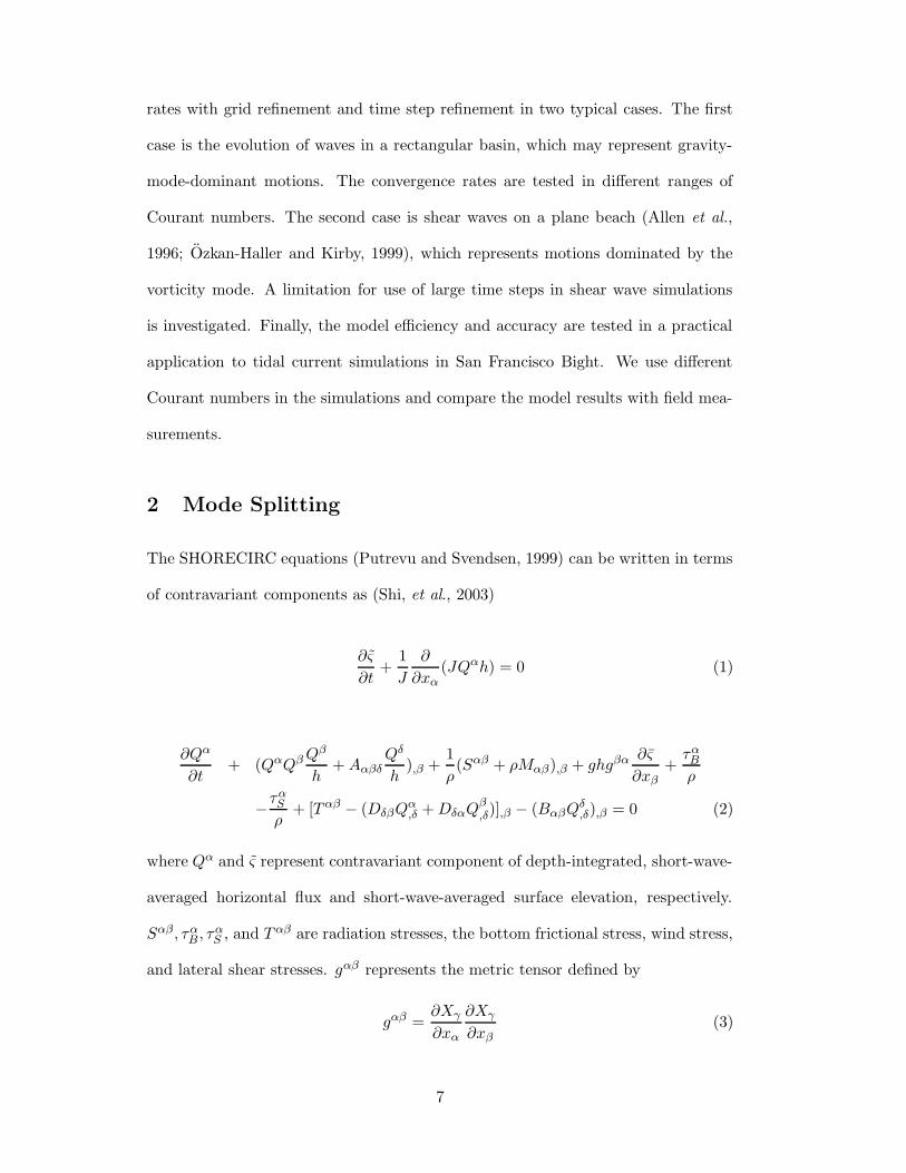
2 Mode Splitting

The SHORECIRC equations (Putrevu and Svendsen, 1999) can be written in terms

of contravariant components as (Shi, et al., 2003)

∂ς

∂t+

1

J

∂

∂xα(JQαh) = 0 (1)

∂Qα

∂t+ (QαQβ Qβ

h+ Aαβδ

Qδ

h),β +

1

ρ(Sαβ + ρMαβ),β + ghgβα ∂ς

∂xβ

+ταB

ρ

−ταS

ρ+ [T αβ − (DδβQα

,δ + DδαQβ,δ)],β − (BαβQδ

,δ),β = 0 (2)

where Qα and ς represent contravariant component of depth-integrated, short-wave-

averaged horizontal flux and short-wave-averaged surface elevation, respectively.

Sαβ, ταB , τα

S , and T αβ are radiation stresses, the bottom frictional stress, wind stress,

and lateral shear stresses. gαβ represents the metric tensor defined by

gαβ =∂Xγ

∂xα

∂Xγ

∂xβ

(3)

7

where Xγ represents horizontal spatial variables in rectangular Cartesian coordi-

nates. The 3-D dispersion effect caused by the vertical variation of horizontal ve-

locity is represented in the terms containing the coefficients A,B,D and M (refer

to Shi et al., 2003 for details).

Equation (2) can be split using the two-step projection method and can be

approximated as follows:

Qα(∗) = Qα(n) + ∆tF α(n)v (4)

Qα(n+1) = −gh∆tgβα

(

∂ς

∂xβ

)(n+1)

+ Qα(∗) (5)

where Qα(∗) is the intermediate flux value computed from incremental changes re-

sulting from the vorticity mode and F αv represents terms dominating the vorticity

mode and is given by

Fαv = −(

QαQβ

h+

AαβδQδ

h),β − 1

ρ(Sαβ + ρMαβ),β − τα

B

ρ+

ταS

ρ

−[T αβ − (DδβQα,δ + DδαQβ

,δ)],β − (BαβQδ,δ),β (6)

Here, we assume the wave force and the variables associated with wave-current

interaction are slowly varying. The 3-D dispersion terms containing the coefficients

A,B,D and M are evaluated using the analytical formulations given in Shi et al.

(2003) with the known values at the previous time step. The turbulence-induced

lateral mixing T αβ and the bottom stress term ταB are also evaluated using the

known values at the previous time level. It should be mentioned that the bottom

friction term could be moved to the gravity mode and solved implicitly in order

to improve the numerical stability (Leendertse and Gritton, 1971). In the present

study, we still keep the friction term in the vorticity mode in order to incorporate

8

short wave effects into the bottom friction (Svendsen et al., 2002). We do not find

any numerical stability problems in our model tests.

Equation (5) presents the gravity mode of the equations with the correction from

the vorticity mode. We now call (5) the gravity mode since Qα(∗) is a known value

obtained from the previous time step. Substituting (5) into the continuity equation

(1) yields a mixed difference-differential equation,

∂ς

∂t=

1

J

∂

∂xα

(

gh∆tJgβα ∂ς(n+1)

∂xβ

)

− 1

J

∂JQα(∗)

∂xα(7)

or

∂ς

∂t=

1

J

∂

∂xα

(

gh∆tJgβα ∂ς(n+1)

∂xβ

)

− 1

J

∂J(Qα(n) + ∆tFα(n)v )

∂xα(8)

Equation (8) is a single parabolic equation with respect to the surface elevation at

the (n + 1) time level. When it is solved the volume flux at time level (n + 1) can

be calculated using (5) or

Qα(n+1) = −gh∆tgβα

(

∂ς

∂xβ

)(n+1)

+ Qα(n) + F α(n)v ∆t (9)

It should be noted that Equation (8) contains both the gravity mode and vor-

ticity mode. The gravity mode appears in implicit form while the vorticity mode

appears explicitly.

3 Numerical Schemes

In order to use McKee et al.’s (1996) ADI scheme for parabolic equations with mixed

derivative and convective terms, we rewrite Equation (8) in a general form as

9

∂ς

∂t= aαβ

∂2 ς

∂xαxβ+ bα

∂ς

∂xα+ c (10)

where

aαβ = gh∆tgαβ (11)

bα =g∆t

J

(

∂Jgαβh

∂xβ

)

(12)

c = − 1

J

∂J(Qα(n) + ∆tFα(n)v )

∂xα(13)

aαβ is a symmetric array, and thus the mixed derivative terms in (10) can be written

as

2a12∂2ς

∂x1∂x2

or

2a21∂2ς

∂x1∂x2

Compared to the general partial differential equation given in McKee et al. (1996),

Equation (10) has an extra term c which can be treated as a source term in the

advection-diffusion equation. In addition, there is no real advection term in the

equation aside from the advection-like term induced by the coordinate distortion.

We follow McKee et al.’s (1996) method to derive the ADI scheme and get a similar

scheme for Equation (10). To get the order of accuracy O(∆t,∆x2α), we discritize the

equation on a uniform spatial mesh in the image plane with ∆x1 = ∆x2 and use a

10

central difference scheme for the advection-like terms. A staggered Arakawa ‘C’ grid

(Arakawa and Lamb, 1977) as shown in Figure 1 is used for surface elevation and

current flux. The difference equations of (10) in the alternating direction implicit

schemes can be written as

[

1 − ra11

2δ2x1

− pb1

2∇x1

]

ς(n+1)∗i,j =

[

1 + ra22δ2x2

+ pb2∇x2+

ra11

2δ2x1

+pb1

2∇x1

+ra22

4δx1x2

]

ςni,j +

∆t

2c (14)

[

1 − ra22

2δ2x2

− pb2

2∇x2

]

ςn+1i,j =

ς(n+1)∗i,j −

[

ra22

2δ2x2

+pb2

2∇x2

]

ςni,j (15)

where r and p are ratios defined by

r = ∆t/(∆x1)2 = ∆t/(∆x2)

2, p = ∆t/(2∆x1) = ∆t/(2∆x2)

and we define the discritization operations

∇x1ςni,j = ςn

i+1,j − ςni−1,j

∇x2ςni,j = ςn

i,j+1 − ςni,j−1

δ2x1

ςni,j = ςn

i+1,j − 2ςni,j + ςn

i−1,j

δ2x2

ςni,j = ςn

i,j+1 − 2ςni,j + ςn

i,j−1

11

δx1x2ςni,j = ςn

i+1,j+1 − ςni+1,j−1 − ςn

i−1,j+1 + ςni−1,j−1

The scheme is the same as that in McKee et al. (1996) except the first order

derivatives are treated by a central difference. McKee et al. (1996) mentioned that

the order of accuracy decays to O(∆t,∆xα) when the first order up-winding scheme

is used for advection terms. Introducing the second order up-winding scheme can

increase to O(∆t,∆x2α). We do not use the suggested scheme because of the fact

that the first order derivatives in our equation are not the real advection terms.

The grid distortion caused advection-like terms are expected to have minor effect

on overall model accuracy under the condition of a smooth curvilinear grid.

To facilitate the description of the boundary condition implementation shown

in next subsection, we give an extended form of the difference equations. Equation

(13) can be written in a tri-diagonal form as

d1 ς(n+1)∗i−1,j + d2 ς

(n+1)∗i,j + d3 ς

(n+1)∗i+1,j = d4 (16)

where

d1 = −ra11

2+

pb1

2(17)

d2 = 1 + ra11 (18)

d3 = −ra11

2− pb1

2(19)

12

d4 = (ra22 − pb2)ςni,j−1 + (ra22 + pb2)ς

ni,j+1 + (1 − 2ra22 − ra11)ς

ni,j

+(ra11

2− pb1

2)ςn

i−1,j + (ra11

2+

pb1

2)ςn

i+1,j

+ra11

4ςni+1,j+1 −

ra11

4ςni+1,j−1 −

ra11

4ςni−1,j+1 +

ra11

4ςni−1,j−1

−p(

Q1(n)i+1,j − Q

1(n)i,j + Q

2(n)i,j+1 − Q

2(n)i,j + ∆t(F 1

v )ni+1,j

−∆t(F 1v )ni,j + ∆t(F 2

v )ni,j+1 − ∆t(F 2v )ni,j

)

−p

(

Q1(n)i+1,j + Q

1(n)i,j

4Ji,j(Ji+1,j − Ji−1,j) +

Q2(n)i,j+1 + Q

2(n)i,j

4Ji,j(Ji,j+1 − Ji,j−1)

)

(20)

Equation (15) can be written as

e1 ς(n+1)i,j−1 + e2 ς

(n+1)i,j + e3ς

(n+1)i,j+1 = e4 (21)

with a corresponding definition for e1, e2, e3 and e4. Equations (16) and (21) consti-

tute linear tri-diagonal systems of equations for ς (n+1)∗ and ς(n+1)i,j , respectively and

can be solved efficiently using elimination method with proper boundary conditions.

Once ς(n+1)i,j is achieved at every elevation point, the current flux Qα(n+1) can be

obtained immediately using Equation (9) at current flux points.

4 Boundary Conditions

There are several types of boundary conditions implemented in the SHORECIRC

model. The use of the mode-splitting and the implicit numerical scheme requires

some changes in boundary condition implementations. Here we concentrate on three

frequently used boundary conditions: flux, elevation, and periodic lateral bound-

aries.

13

4.1 Specified Flux Boundary Condition

A specified flux boundary condition in generalized curvilinear coordinates can be

easily expressed by using the contravariant component of current flux:

Q1 = Q10 at west or east boundaries (22)

Q2 = Q20 at south or north boundaries (23)

where Qα0 (α = 1, 2) represents given depth-integrated flux values at boundaries.

The case of an impermeable wall boundary is represented by the special case Qα0 = 0.

On a staggered grid, only flux points are arranged at the boundaries where the

specified flux boundary conditions (22) or (23) are satisfied, e.g., Q1-points at east

or west boundaries and Q2-points at south or north boundaries. Substituting the

boundary conditions (22) or (23) in Equations (9) and (10) results in some changes

in the coefficients (d1, d2, d3, d4) or (e1, e2, e3, e4) at the boundary points. At the

west boundary points,

d1 = 0 (24)

d2 = 1 +1

2ra11 (25)

d3 = −ra11

2− pb1

2(26)

14

d4 = (ra22 − pb2)ςni,j−1 + (ra22 + pb2)ς

ni,j+1 + (1 − 2ra22 − ra11)ς

ni,j

+ra11

2ςni+1,j +

ra11

4ςni+1,j+1 −

ra11

4ςni+1,j−1

−p(

Q1(n)i+1,j − Q1

0 + Q2(n)i,j+1 − Q

2(n)i,j

+∆t(F 1v )ni+1,j + ∆t(F 2

v )ni,j+1 − ∆t(F 2v )ni,j

)

−p

(

Q1(n)i+1,j + Q1

0

4Ji,j(Ji+1,j − Ji,j) +

Q2(n)i,j+1 + Q

2(n)i,j

4Ji,j(Ji,j+1 − Ji,j−1)

)

(27)

Corresponding changes in (d1, d2, d3, d4) can be made for the east boundaries and

changes in (e1, e2, e3, e4) for the south and north boundaries.

4.2 Specified Surface Elevation Boundary Condition

On a staggered gird, only surface elevation points are distributed at the specified

elevation boundaries. Substituting the elevation boundary condition

ς = ς0 (28)

into (16) for east or west boundaries or (21) for south or north boundaries directly

yields the new tri-diagonal coefficients: at the west boundaries, for example, we get

d′

1 = 0, d′

2 = d2, d′

3 = d3, and d′

4 = d4 − d1 ς0 where ()′

represents new coefficients.

4.3 Periodic Boundary Condition

For spatially periodic boundary conditions, only surface elevation points are de-

fined at the boundaries. Linear periodic tridiagonal systems can be constructed

using (16) for the east-west periodic boundary and (21) for the south-north periodic

boundary. For applications using the periodic boundary conditions, wave forcing,

15

bathymetry, computational grid and other spatial distributed variables should also

have the periodic properties related to the periodic boundary conditions.

5 Model Applications

5.1 Tests on Convergence Rates in a Gravity-mode-dominant Case

McKee et al. (1996) used the traditional von Neumann method to prove that the

scheme is unconditionally stable when the coefficients in the parabolic equation are

constant. Most recently, in’t Hout and Welfert (2007) derived new linear stability

results for ADI schemes applied to general parabolic convection-diffusion equations

with mixed derivative terms. They also showed that the ADI schemes with cross-

derivative discritizations are unconditionally stable. Convergence rates with time

refinement were also investigated in their study. As a specific application of this

kind of ADI schemes, the discritized equations in our study need to be tested on

convergence rates with both time and grid refinement. The convergence rates with

grid refinement is especially important for our model since variable grid spacing is

used in a grid system.

Following Shi et al. (2001), we perform simple tests of the evolution of waves in a

rectangular basin. The conditions used in the numerical experiments are the same as

in Shi et al. (2001), including a basin dimension of 20×20m , 0.5m water depth and

a motionless Gaussian bump as the initial condition. To test the convergence with

time discritization, we use a sequence of time steps, i.e., ∆t/i, where ∆t = 0.5 and

i = 1, 2, ...20. We choose two different grid spacings, i.e., ∆x =0.1 m and 0.8 m, for

all the time steps. The convergence rates with time refinement are demonstrated by

the RMS differences of simulated surface elevations at t = 20s. The RMS difference

16

of surface elevation is defined by

RMSp =

√

∑

(ζp(i, j) − ζp+1(i, j))2

(m × n)2(29)

where ζp represents the calculated surface elevations in the case p and (m,n) are

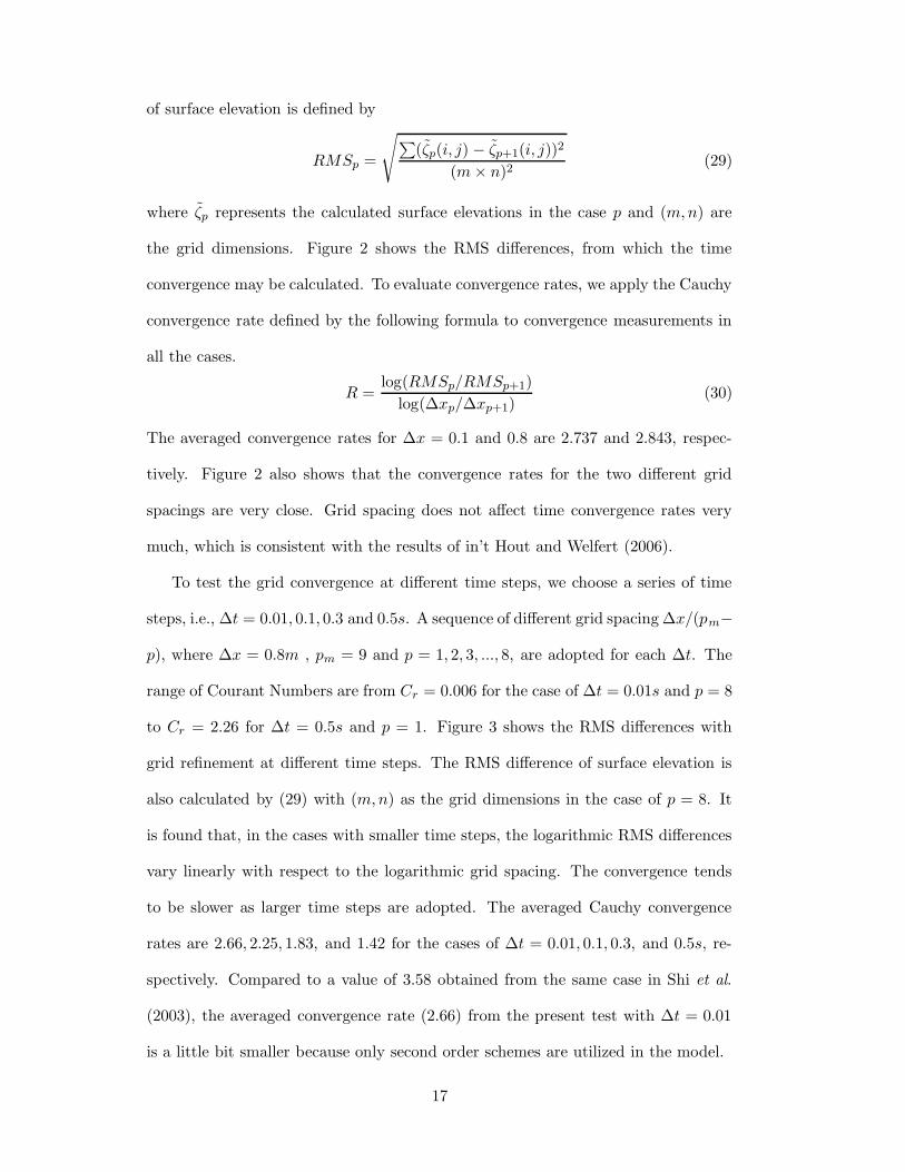
the grid dimensions. Figure 2 shows the RMS differences, from which the time

convergence may be calculated. To evaluate convergence rates, we apply the Cauchy

convergence rate defined by the following formula to convergence measurements in

all the cases.

R =log(RMSp/RMSp+1)

log(∆xp/∆xp+1)(30)

The averaged convergence rates for ∆x = 0.1 and 0.8 are 2.737 and 2.843, respec-

tively. Figure 2 also shows that the convergence rates for the two different grid

spacings are very close. Grid spacing does not affect time convergence rates very

much, which is consistent with the results of in’t Hout and Welfert (2006).

To test the grid convergence at different time steps, we choose a series of time

steps, i.e., ∆t = 0.01, 0.1, 0.3 and 0.5s. A sequence of different grid spacing ∆x/(pm−

p), where ∆x = 0.8m , pm = 9 and p = 1, 2, 3, ..., 8, are adopted for each ∆t. The

range of Courant Numbers are from Cr = 0.006 for the case of ∆t = 0.01s and p = 8

to Cr = 2.26 for ∆t = 0.5s and p = 1. Figure 3 shows the RMS differences with

grid refinement at different time steps. The RMS difference of surface elevation is

also calculated by (29) with (m,n) as the grid dimensions in the case of p = 8. It

is found that, in the cases with smaller time steps, the logarithmic RMS differences

vary linearly with respect to the logarithmic grid spacing. The convergence tends

to be slower as larger time steps are adopted. The averaged Cauchy convergence

rates are 2.66, 2.25, 1.83, and 1.42 for the cases of ∆t = 0.01, 0.1, 0.3, and 0.5s, re-

spectively. Compared to a value of 3.58 obtained from the same case in Shi et al.

(2003), the averaged convergence rate (2.66) from the present test with ∆t = 0.01

is a little bit smaller because only second order schemes are utilized in the model.

17

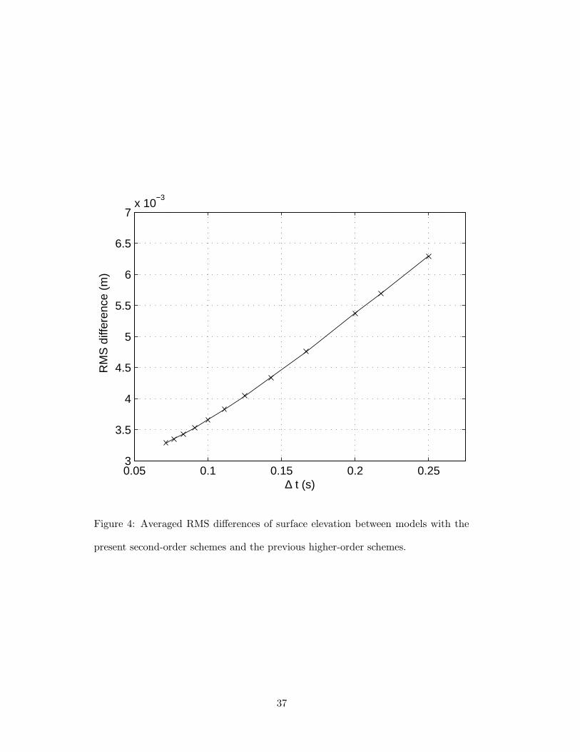
In the development of the fully nonlinear Boussinesq models (Wei and Kirby,

1995, Shi et al., 2001), higher-order numerical schemes in both space and time were

used because the truncation errors of a second-order approximation may contami-

nate the real dispersive terms in the Boussinesq equations. This should not be a

problem in the present model because the SHORECIRC equations do not include

terms involving higher-order derivatives. However, It should be noted that the

present numerical schemes, with first-order accuracy in time and second order accu-

racy in space, may cause numerical diffusion that may affect calculations of physical

diffusion caused by turbulent mixing. To examine the accuracy of the second-order

ADI schemes, we make a numerical test against the previous explicit scheme which

is second-order in time and fourth-order in space (Shi et al., 2003). The previous

model with the higher order scheme is run in the same application with ∆x = 0.4m

and ∆t = 0.04s. The result for surface elevation is compared to the present model

results with a sequence of time steps. Figure 4 shows the averaged (over all grid

points) RMS errors of surface elevation between the previous model result and re-

sults from the present model at different time steps. It shows that the accuracy

of the present model with second-order schemes is lower than the previous model.

But it is acceptable for regular hydrodynamic simulations. For simulations with

complex geometries, the Courant numbers are suggested not to exceed 10 because

of the “ADI effect” (Casulli and Cheng, 1992).

5.2 Vorticity-mode-dominant Case: Modeling of Nearshore Shear

Waves

Studies on surfzone dynamics have revealed the existence of a variety of low-frequency

motions including edge waves, surf beat and shear waves at the shoreline (Noyes et

al., 2005). Amongst these low-frequency waves are shear waves, which are manifes-

tation of shear instability of the mean longshore current. Shear waves are dominated

18

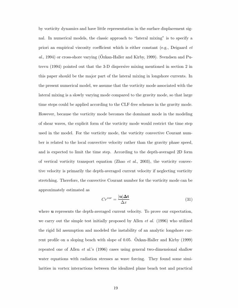
by vorticity dynamics and have little representation in the surface displacement sig-

nal. In numerical models, the classic approach to “lateral mixing” is to specify a

priori an empirical viscosity coefficient which is either constant (e.g., Deigaard et

al., 1994) or cross-shore varying (Ozkan-Haller and Kirby, 1999). Svendsen and Pu-

trevu (1994) pointed out that the 3-D dispersive mixing mentioned in section 2 in

this paper should be the major part of the lateral mixing in longshore currents. In

the present numerical model, we assume that the vorticity mode associated with the

lateral mixing is a slowly varying mode compared to the gravity mode, so that large

time steps could be applied according to the CLF-free schemes in the gravity mode.

However, because the vorticity mode becomes the dominant mode in the modeling

of shear waves, the explicit form of the vorticity mode would restrict the time step

used in the model. For the vorticity mode, the vorticity convective Courant num-

ber is related to the local convective velocity rather than the gravity phase speed,

and is expected to limit the time step. According to the depth-averaged 2D form

of vertical vorticity transport equation (Zhao et al., 2003), the vorticity convec-

tive velocity is primarily the depth-averaged current velocity if neglecting vorticity

stretching. Therefore, the convective Courant number for the vorticity mode can be

approximately estimated as

Crvor =|u|∆t

∆x(31)

where u represents the depth-averaged current velocity. To prove our expectation,

we carry out the simple test initially proposed by Allen et al. (1996) who utilized

the rigid lid assumption and modeled the instability of an analytic longshore cur-

rent profile on a sloping beach with slope of 0.05. Ozkan-Haller and Kirby (1999)

repeated one of Allen et al.’s (1996) cases using general two-dimensional shallow

water equations with radiation stresses as wave forcing. They found some simi-

larities in vortex interactions between the idealized plane beach test and practical

19

shear wave simulations associated with the SUPERDUCK field experiment. Allen

et al. (1996) pointed out that, in their numerical solutions, shear wave behavior

may vary over the full range from periodic to chaotic with different bottom fiction

coefficients and domain size. For comparison, we conducted a shear wave simulation

on a plane beach which was used by Ozkan-Haller and Kirby (1999). The computa-

tional domain is set to be 350m and 3600m in cross-shore and alongshore directions,

respectively. The grid sizes are chosen as 5m in both directions. Wave forcing, i.e.,

radiation stresses, is calculated from the REF/DIF-1 wave model (Kirby, et al.,

2002). Periodic boundary conditions are used in the alongshore direction. We use

the quadratic-type bottom stress formulation (Svendsen et al., 2002) with a constant

bottom friction coefficient fcw = 0.003 with which we get a vorticity pattern similar

to that in Ozkan-Haller and Kirby (1999). For lateral mixing, there is no specifica-

tion of a lateral mixing parameter needed since the lateral mixing mainly depends

on the 3D dispersion evaluated by the local vertical profiles of the calculated current

velocities. To trigger shear waves on the longshore uniform plane beach, we used

the same strategy as that used in Ozkan-Haller and Kirby (1999), and introduce

small perturbations in the initial longshore velocity v given by

v(x, y, t = 0) =ε

max(f)f, (32)

where ε is a small parameter and the function f is given by

f =

ND∑

j=1

cos(2πjy

Ly+ 2πφj) (33)

in which, ND is the number of times the most unstable wavelength fits into the

modeling domain and φj is a random phase function between −1 and 1. Ly rep-

resents the domain length in the longshore direction. Following Ozkan-Haller and

Kirby (1999), we adopted ND = 16 that ensures the generations of the most unsta-

ble wavelength as well as all longer wavelengths in the modeling domain. We use

20

ε = 1 × 10−3, which is orders of magnitude larger than that used in Ozkan-Haller

and Kirby (1999), in order to accelerate the process of shear wave generation.

Figure 5 shows the wave height distribution predicted by the REF/DIF-1 wave

model and the longshore current profile (longshore-averaged) along with the water

depth h for a monochromatic wave with a frequency of 0.10 Hz and wave direction

of 20◦ at 17.5m water depth. It is found that the longshore-averaged current profile

does not vary much when different time steps are applied. In Figure 6, we show

a snapshot of the computed wave-induced nearshore currents (arrows) and vertical

vorticity (color) distribution at 180 minutes. Compared with the vorticity fields in

Ozkan-Haller and Kirby’s (1999) case, the length of the shear waves and vorticity

patterns look comparable to their results at the time before more vortices merge

together.

We now concentrate on testing of numerical convergence in shear wave simu-

lations using different temporal resolutions. A sequence of different time steps is

selected, i.e., ∆t × 2p, where ∆t = 0.125s and p = 0, 1, ... , 6. The corresponding

gravity wave Courant numbers (the maximum values in the computational domain)

for the sequence of time steps are from 0.16 to 10.48 according to

Crgra|max =

√ghmax∆t

∆x(34)

The maximum Courant numbers for vorticity convection can be also evaluated based

on (31):

Crvor|max =|u

max|∆t

∆x(35)

where umax represents the maximum current velocity vector in the whole computa-

tional domain. To characterize the strength of shear waves in the numerical results,

we use the enstrophy integrated over the computational domain:

Φ =

∫ Lx

0

∫ Ly

0

ωzωz

2dxdy (36)

21

where ωz is the depth-averaged vertical vorticity for shear waves. Model convergence

with time discritization in the shear wave simulations can be evaluated by ∆Φ =

Φp+1 −Φp with respect to ∆t, Crvor or Crgra. The convergence rate with time step

refinement is shown in Figure 7 in which the gravity wave Courant numbers are

labeled on the top axis while the corresponding vorticity wave Courant numbers are

labelled on the bottom axis. The model is convergent with the time step refinement.

The shear waves can be modeled using larger gravity wave Courant numbers, but

time steps are still restrained by the vorticity wave Courant numbers. It is found

that vorticity wave Courant numbers should be less than 1 in shear wave simulations

using the present model, otherwise, numerical instability would occur.

5.3 Application to San Francisco Bight

In ocean-exposed coastal regions, waves, nearshore circulation and sediment trans-

port are usually affected by large-scale motions such as tides, ocean circulation

and storm surges. In modeling of nearshore processes at open coasts, open bound-

ary conditions associated with the large-scale motions are needed by the nearshore

models and are usually unknown if without measurements. It is a challenge how

to incorporate far field data into nearshore models. Besides model coupling tech-

niques performed between the nearshore models and large-scale models to apply

the far field data, one efficient method is to extend the nearshore models for rela-

tively larger scale applications. For the nearshore circulation model, for instance,

the model extension can be made by approximately adding some large-scale forc-

ing components such as tidal boundary conditions, wind stresses and the Coriolis

force. The extended nearshore circulation model will become more computationally

expensive because all the existing nearshore model features are included. The im-

provement of computational efficiency for an extended nearshore circulation model

is therefore important. In the following model application to San Francisco Bight,

22

we demonstrate the capability of the present model to simulate tidal currents and

nearshore simulations in large-scale computational domains with high efficiency.

San Francisco Bight is characterized by broad shoals and narrow channels in a

complicated estuary system. Because of large variations of depth distribution at the

ebb tidal delta and the deep Golden Gate channel, the hydrodynamic conditions

involving wave-current interaction are extremely complicated. Strong tidal currents

at the entrance of the Golden Gate significantly affect wave transformation and lead

to a complex, longshore-inhomogeneous wave climate which, in turn, leads to vari-

able sediment transport processes at the inlet and nearshore regions. Recent studies

on the beach evolution (Barnard et al., 2004) indicated that the shape and location

of the ebb tidal shoal directly links to an erosional ‘hot spot’ on the southern end

of Ocean Beach. Previous systematic numerical studies on hydrodynamics in San

Francisco Bay have been carried out with a focus on tidal currents and residual flows

inside the bay (Cheng and Casulli, 1982, Cheng et al., 1993, and others). However,

nearshore hydrodynamic processes were rarely linked to the large-scale simulations.

As the first step to develop a model system predicting waves, nearshore circulations

and sediment transport in the San Francisco coastal region, we concentrate on mod-

eling tidal currents and wave-induced nearshore circulations with an aim to examine

the model efficiency in such a large-scale computational domain.

Figure 8 shows the computational grid generated using the CoastGrid software

(Shi, 2007). The maximum grid size is 1, 320m at the offshore boundaries. Finner

grid cells are applied at the coastline and the inlet (see blow-up figure 9) with a min-

imum grid size of 19m. The computational domain covers the whole San Francisco

Bay and the adjacent Pacific shelf. Specifically, the western offshore boundary is

located at the shelf edge and southern and northern boundaries are near Monterey

Bay and Pt. Reyes, respectively. The tidal boundary conditions are applied at

the western, southern and northern open boundaries. Eight harmonic constituents,

23

including M2,K1, O1, S2, P1, N2, Q1 and K2, are obtained from harmonic analysis

of tidal data observed at the Pt. Reyes Buoy and the Monterey Buoy. The con-

stituents are used to estimate the tidal elevations at the western, northern and

southern boundaries. Based on historical records, a river discharge of 400m3/sec

is specified for each of the Sacramento River and San Joaquin River located at the

north-west end of the domain. Wind is taken into account using the wind data from

the NOAA San Francisco station 46026 uniformly over the whole domain.

The bottom stress formulation (Svendsen et al., 2002) with a constant bottom

friction coefficient fw = 0.0020 is adopted in the tidal current simulation. The

turbulent mixing coefficients in the eddy viscosity formulation are chosen as the

same values as in Svendsen et al. (2002).

We carried out a six-month simulation of tides in which the ADCP data are

available at a location in the Golden Gate channel as shown in Figure 10 (marked

‘SITE’). The simulation time period is from January 1 to June 30, 1998. Different

Courant numbers are used in the tests. Surface wave forcing is not taken into account

in the case. It is found that the model/data comparisons of surface elevation at the

Golden Gate station are satisfactory in the six-month time period except for a

two-day spin-up period. Figure 11 shows the model/data comparisons of surface

elevation with Courant numbers of 10 and 100, respectively. It can be seen that the

two numerical results are basically identical and both of them agree well with the

data. An evaluation of the correlation between model results and data shows that

the regression coefficients R2 for surface elevation are 0.945 for Cr = 10 and 0.942 for

Cr = 100. Figure 12 shows comparisons of depth-averaged tidal currents modeled

from Cr = 10 (solid line) and Cr = 100 (dashed line) against the depth-averaged

ADCP data. It is shown that the tidal currents modeled from different Courant

numbers are basically close, with the two line types indistinguished in the figure.

The regression coefficient R2, which is calculated using a discontinuous ADCP data

24

of depth-averaged velocity amplitude, is 0.550 for Cr = 100 and 0.553 for Cr = 10 in

the six-month time period. Figure 13 and Figure 14 demonstrate snapshots of tidal

current fields at flood tide and ebb tide, respectively. Strong tidal currents, with the

maximum depth-averaged velocity of over 2m/s, can be found at the Golden Gate

channel. Several vortex cells are identified at upper Ocean Beach, Baker Beach and

Marin Headlands.

Wave-induced nearshore circulation can be modeled by coupling a circulation

model and a wave model. In the San Francisco Bight application, we coupled the

present circulation model and the spectral wave model SWAN (Booij et al., 1999).

The non-stationary mode of SWAN was adopted in a two-way coupling system. As a

model test, wave-induced nearshore circulation at Ocean Beach is simulated under

common storm wave conditions with 3m significant wave height, and 15 seconds

peak period in deep water. A constant wind field with 10m/s from 300◦ (Nautical)

is used in the simulation. Figure 15 shows wave-induced longshore currents along

the Ocean Beach. The current magnitude is about 1m/s which is comparable to

the magnitude of tidal currents in this region.

It should be mentioned that, most recently, the U.S. Geological Survey (USGS)

began a seasonal surveying campaign at Ocean Beach. Nearshore bathymetry data

has been collected bi-annually, with additional surveys to coincide with instrument

deployments in the offshore and surfzone regions. The SHORECIRC model with

the fast numerical schemes developed in this study has been coupled with the wave

model SWAN and a sediment model to investigate waves, currents and sediment

transport in San Francisco Bight. The model results validated using the field data

will be reported in the near future, in conjunction with a more detailed investigation

of waves, nearshore circulations and sediment transport in San Francisco Bight and

its adjacent open beaches.

25

6 Conclusions and Remarks

A mode-splitting method is used in the Quasi-3D nearshore circulation model SHORE-

CIRC with an aim to improve the model efficiency. Using the two-step projection

method, we separate the gravity mode and the vorticity mode which represent re-

spectively the fast motions and the slow motions in the nearshore hydrodynamic

system. The vorticity mode of the equations is used to compute the intermediate

flux value from incremental changes resulting from wave forcing, 3-D dispersion ef-

fect caused by the vertical nonuniformity of current velocity, the turbulence-induced

lateral mixing and the bottom friction. We use an explicit scheme for the vortic-

ity mode, especially, the 3-D dispersion terms are evaluated based on analytical

formulations and using the known values of current velocity at previous time level.

The gravity mode includes the pressure gradient terms, which represents incremental

changes resulting from the pressure gradient. The final equation for the combination

of the gravity mode and vorticity mode is derived by substituting the momentum

equations into the continuity equation and it becomes a single parabolic equation

with respect to surface elevation. The parabolic type equation can be solved im-

plicitly using the traditional ADI scheme, specifically in the present model, McKee

et al.’s (1996) ADI scheme for parabolic equations is used to deal with the mixed

derivative and convective terms caused by the coordinate transformation.

To test the model convergence rates with the refinement of grid spacing and time

step, we carried out two typical cases, i.e., the evolution of waves in a rectangular

basin which is a gravity-mode-dominant case, and the simulation of shear waves on

a plane beach which is a case dominated by the vorticity mode. The case of wave

evolution shows that the averaged Cauchy convergence rates with grid refinement

are a little lower than the previous SHORECIRC model (Shi et al., 2003) but are

still satisfactory considering the second order schemes utilized in the model. In the

26

case of the shear wave simulation, we found that relatively larger time steps (gravity

convective Courant number > 1) can be used but the time steps are restricted by the

explicit form of the vorticity mode. The vorticity convective Courant number that

is a function of the local convective velocity rather than the gravity phase speed,

limits the time steps. The test shows the model is convergent with the time step

refinement and the vorticity wave Courant numbers should not exceed 1 in shear

wave simulations.

Model application to San Francisco Bight indicates that the model has the ca-

pability of large scale modeling with good efficiency. For the present application

grid with dimensions of 291 × 180, the time step is 10.8 seconds for Cr = 10 or 108

seconds for Cr = 100. On a 64-bit linux system with a single processor of 2.0 GHz

and a memory of 2 GB, the model with Cr = 10 takes about 60.8 hours, or about 6

hours with Cr = 100, for a 365-day simulation of tidal currents, without coupling of

the wave and sediment models. With the SWAN model coupled in the system, the

efficiency of the coupled model system mainly depends on the SWAN model setup

and may become computational expensive, especially when a smaller Courant num-

ber is chosen. However, it is obvious that the model efficiency is greatly improved

using the present numerical schemes compared to the previous SHORECIRC model

with a limitation of Cr < 1.

The model is valided using the ADCP data measured near the Golden Gate

channel in 1998. Model results of tidal surface elevations and tidal currents are in

good agreements with the data. A test using different Courant numbers in the sim-

ulations shows that the Courant number can be increased to 100 without significant

loss in accuracy. Finally, wave-induced longshore currents along the open beaches

are calculated by coupling the present model and the wave model SWAN.

The basic hypothesis for the mode-splitting is that the nearshore motions can

be separated into fast motions dominated by the gravity mode and slow motions

27

dominated by the vorticity mode. However, nearshore processes with wave-current

interactions are complex and may involve a large range of time scales. In some cases

(e.g., rip current simulation using SHORECIRC, Haas, et al., 2003), the time scale

for the current field variation to respond to wave-current interaction may be small,

which would limit the use of larger time steps in the nearshore circulation model.

More tests for the time step limitation should be carried out in a wide range of

nearshore applications in the future.

In the extension of the present model to large-scale applications, we neglect

the baroclinic motions that may be important in estuarine or some coastal regions.

Therefore, the usage of the model extension at this stage should be confined to

applications in which the barotropic tides are dominent far field boundary conditions

in the nearshore circulation modeling.

The CFL-free ADI scheme does not mean that large Courant numbers could

be used for gravity wave motions. Because of the “ADI effect” caused by complex

geometries (Casulli and Cheng, 1992), the Courant numbers were suggested not to

exceed 10 to get accurate results. Although we use Cr = 100 in the case of San

Francisco Bight with a good accuracy, more numerical experiments may be needed

for different geometries.

Acknowledgments. This study was supported by Office of Naval Research, Coastal

Geosciences Program (N00014-05-1-0423) and U.S. Geological Survey, Coastal Evo-

lution: Process-based Multi-scale Modeling Project.

References

Arakawa, A. and Lamb, V. R., 1977, Computational design of the basic dynamical

processes of the UCLA general circulation model. Methods in Computational

28

Physics, Vol. 17, Academic Press, 174-265.

Allen, J. S., Newberger, P. A. and Holman, R. A., 1996, Nonlinear shear instabili-

ties of alongshore currents on plane beaches, J. Fluid Mech., 181-213.

Barnard, P. L., Hanes, D. M., and Ruggiero, P., 2004, The relative effects of wave

climatology and tidal currents on beach processes adjacent to a major tidal

inlet, Ocean Beach, San Francisco, California, AGU, Fall Meeting 2004, San

Francisco, abstract published in EOS Transaction AGU, 85 (47), Abstract

OS24A-08.

Bleck, R. and Smith, L. T., 1990, A wind-driven isopycnic coordinate model of the

north and equatorial Atlantic Ocean 1. Model development and supporting

experiments, J. Geophys. Res., 95, 3273-3285.

Booij, N., Ris, R. C., and Holthuijsen, L. H., 1999, A third-generation wave model

for coastal regions. Part 1: Model description and validation, J. Geophys.

Res., 104 (C4), 7649-7666.

Bowen A. J., Inman D. L., Simmons V. P., 1968, Wave set-down and set-up, J.

Geophys. Res., 73, 2569-2577.

Bowen, A. J., 1969, The generation of longshore currents on a plane beach, J. Mar.

Res., 27, 206-215.

Cheng, R. T. and Casulli, V., 1982, On Lagrangian residual currents with applica-

tions in South San Francisco Bay, California, Water Resources Research, 18,

1652-1662.

Cheng, R. T., Casulli, V., and Cartner, J. W., 1993, Tidal, Residual, Intertidal

Mudflat (TRIM) model and its applications to San Francisco Bay, California,

Estuarine, Coastal and Shelf Science, 36, 235-280.

29

Casulli, V. and Cheng, R. T., 1992, Semi-implicit finite difference methods for

three-dimensional shallow water flow, International Journal for Numerical

Methods in Fluids, 15, 629-648.

Casulli, V. and Zanolli, P., 2002, Semi-implicit numerical modeling of nonhydro-

static free-surface flows for environmental problems, Mathematical and Com-

puter Modeling, 36, 1131-1149.

Deigaard, R., Christensen, E. D., Damgaard, J. S. and Fredsoe, J., 1994, Numer-

ical simulation of finite amplitude shear waves and sediment transport, 24th

International Conference on Coastal Engineering, ASCE, Reston, Va.

Dukowicz J. K. and Smith, R. D., 1994, Implicit free-surface method for the Bryan-

Cox-Semtner ocean model, J. Geophys. Res., 99, C4, 7991-8014.

Fischer, H. B., 1978, On the tensor form of the bulk dispersion coefficient in a

bounded skewed shear flow, J. Geophys. Res., 83, 2373-2375.

Haas, K., Svendsen, I. A., Haller, M. C. and Zhao, Q., 2003, Quasi-three-dimensional

modeling of rip current systems, 108, C7, 3217, doi: 10.1029/2002JC001355.

Higdon, R. L., de Szoeke, R. A., 1997, Barotropic-baroclinic time splitting for

ocean circulation modeling, J. Comp. Phys., 135, 31-53.

in’t Hout, K. J. and Welfert, B. D., 2007, Stability of ADI schemes applied to

convection-diffusion equations with mixed derivative terms, Applied Numerical

Mathematics, 57, 19-35.

Killworth, P. D., Stainforth, D., Webb, D. J., and Paterson, S. M., 1991, The devel-

opment of a free-surface Bryan-Cox-Semtner ocean model, J. Phys. Oceanogr.,

21, 1333-1348.

30

Kirby, J. T., Dalrymple, R. A. and Shi, F., 2002, Combined Refraction/Diffraction

Model REF/DIF 1, Version 2.6. Documentation and User’s Manual, Research

Report No.CACR-02-02, Center for Applied Coastal Research, Department of

Civil and Environmental Engineering, University of Delaware, Newark.

Leendertse, J. J. and Gritton, E. C., 1971, A water quality simulation model for

well-mixed estuaries and coastal sea, In: Computation Procedures, R-708-

NYC Vol II, The Rand Corporation, New York, pp. 29-33.

Longuet-Higgins, M. S. and Stewart, R. W., 1964, Radiation stress in water waves,

a physical discussion with application, Deep Sea Res., 11, 529-563.

Longuet-Higgins, M. S., 1970, Longshore currents generated by obliquely incident

sea waves, 1, J. Geophys. Res., 75, 6778-6789.

McKee, S. and Mitchell, A. R., 1970, Alternating direction methods for parabolic

equations in two space dimensions with a mixed derivative, Computer J., 133,

81-86.

McKee, S., Wall, D. P., and Wilson, S. K., 1996, An alternating direction implicit

scheme for parabolic equations with mixed derivative and convective terms, J.

Comput. Phys., 126, 64-76.

Noyes, J. T., Guza, R. T., and Feddersen, F., 2005, Model-data compatrsons of

shear waves in the nearshore, J. Geophys. Res., 110, C05019, doi: 10.1029/2004JC002541

Oberhuber, J. M., 1993, Simulation of the Atlantic circulation with a coupled sea ice

- mixed layer - isopycnal general circulation model, Part I. Model description,

J. Phys. Oceanogr. 23, 808.

Ozkan-Haller, H. T. and Kirby, J. T., 1999, Nonlinear evolution of shear instabilities

of the longshore current: A comparison of observations and computations, J.

31

Geophys. Res., 104, C11, 25,953-25,984.

Putrevu, U. and Svendsen, I. A., 1999, Three-dimensional dispersion of momentum

in wave-induced nearshore currents, Eur. J. Mech. B/Fluids, 18, 83-101.

Sancho, F. E. and Svendsen, I. A., 1998, Shear waves over longshore nonuniform

barred beaches, In Proc. 26th Int. Conf. on Coast. Engrg., Copenhagen,

230-243.

Shchepetkin, A. F. and McWilliams, J. C., 2005, The regional oceanic modeling

system (ROMS): a split-explicit, free-surface, topography-following-coordinate

oceanic model, Ocean Modeling, 9, 347-404.

Shi, F., Dalrymple R. A., Kirby, J. T., Chen, Q. and Kennedy, A., 2001, A fully

nonlinear Boussinesq model in generalized curvilinear coordinates, Coastal En-

gineering, 42, 237-258.

Shi, F., Svendsen, I. A., Kirby, J. T., and Smith, J. M., 2003, A curvilinear version

of a quasi-3D nearshore circulation model, Coastal Engineering, 49, 99 - 124.

Shi, F., 2007, CoastGrid, a software for curvilinear grid generation, Report No.

CACR-07-01, Cent. for Appl. Coastal Res., Univ. of Del., Newark, Del.

Smith, R., 1997, Multi-mode models of flow and of solute dispersion in shallow

water. Part 3. Horizontal dispersion tensor for the velocity, J. Fluid Mech.,

352, 331-340.

Svendsen, I. A. and Putrevu, U., 1994, Nearshore mixing and dispersion, Proc.

Roy. Soc. Lond. A, 445, 561-576.

Svendsen, I. A., Haas, K., and Zhao, Q., 2002, Quasi-3D nearshore circulation

model SHORECIRC, CACR Report No. CACR-02-01, Cent. for Appl. Coastal

Res., Univ. of Del., Newark, Del.

32

Taylor, G. I., 1953, Dispersion of soluble matter in solvent flowing slowly through

a tube, Proc. Roy. Soc. Lond. A, 219, 186-203.

Taylor, G. I., 1954, The dispersion of matter in a turbulent flow through a pipe,

Proc. Roy. Soc. Lond. A, 219, 446-468.

van Dongeren, A. R. and Svendsen, I. A., 2000, Nonlinear and 3D effects in leaky

infragravity waves, Coastal Engineering, 41, 467-496.

Warming, R. F. and Beam, R. M., 1979, An extension of A-stability to alternating

direction methods, BIT, 19, 395-417.

Wei, G., Kirby, J.T., 1995, A time-dependent numerical code for the extended

Boussinesq equations, J. Waterw., Port, Coastal Ocean Eng., 121 (5), 251-

261.

Yu, J., Slinn, D. N., 2001, Effects of wave-current interaction on rip currents, J. of

Geophys. Res., 108, C3, 3088, doi:10.1029/2001JC001105.

Zhao, Q., Svendsen, I. A. and Haas, K. A., 2003, Three-dimensional effects in shear

waves, J. of Geophys. Res., 108, C8, 3270, doi: 10.1029/2002JC001306.

33

Figure 1: Staggered Arakawa ‘C’ grid in x1 − x2 plane (cross - ζ point, circle - Q1

point, box - Q2 point)

34

0.1 0.2 0.3 0.4 0.5 0.6

10−4

10−3

∆ t (s)

RM

S d

iffer

ence

(m

)

dx = 0.8 mdx = 0.1 m

Figure 2: RMS differences with time refinement using two different grid spacings.

35

0.1 0.15 0.2 0.25 0.3 0.35 0.4

10−5

10−4

10−3

10−2

∆ x (m)

RM

S d

iffer

ence

(m

)

dt = 0.01 sdt = 0.1 sdt = 0.3 sdt = 0.5 s

Figure 3: RMS differences with grid refinement using different time steps.

36

0.05 0.1 0.15 0.2 0.253

3.5

4

4.5

5

5.5

6

6.5

7x 10

−3

∆ t (s)

RM

S d

iffer

ence

(m

)

Figure 4: Averaged RMS differences of surface elevation between models with the

present second-order schemes and the previous higher-order schemes.

37

0 50 100 150 200 250 300 350−20

−15

−10

−5

0

−h

(m)

0 50 100 150 200 250 300 3500

2

4

6

wav

e he

ight

(m

)

0 50 100 150 200 250 300 350−0.5

0

0.5

1

1.5

aver

aged

v (

m/s

)

x (m)

Figure 5: Simulation of longshore currents on a plane beach. (top) bathymetry with

a slope of 0.05, (middle) wave height from the REF/DIF-1 wave model, (bottom)

longshore current profile

38

Figure 6: Snapshot of current field (arrow) and vorticity (color, s−1) for a plane

beach

39

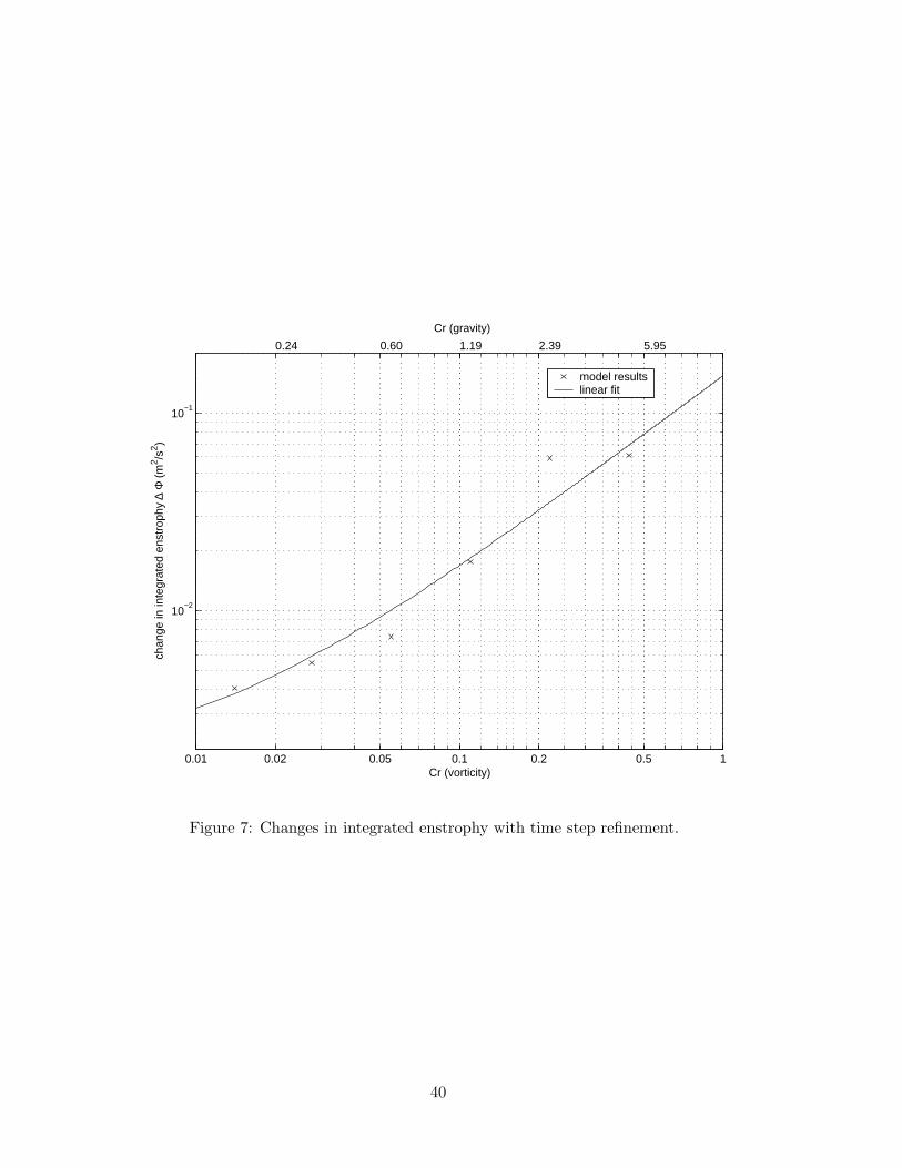
0.01 0.02 0.05 0.1 0.2 0.5 1

10−2

10−1

Cr (vorticity)

chan

ge in

inte

grat

ed e

nstr

ophy

∆ Φ

(m

2 /s2 )

0.24 0.60 1.19 2.39 5.95

Cr (gravity)

model resultslinear fit

Figure 7: Changes in integrated enstrophy with time step refinement.

40

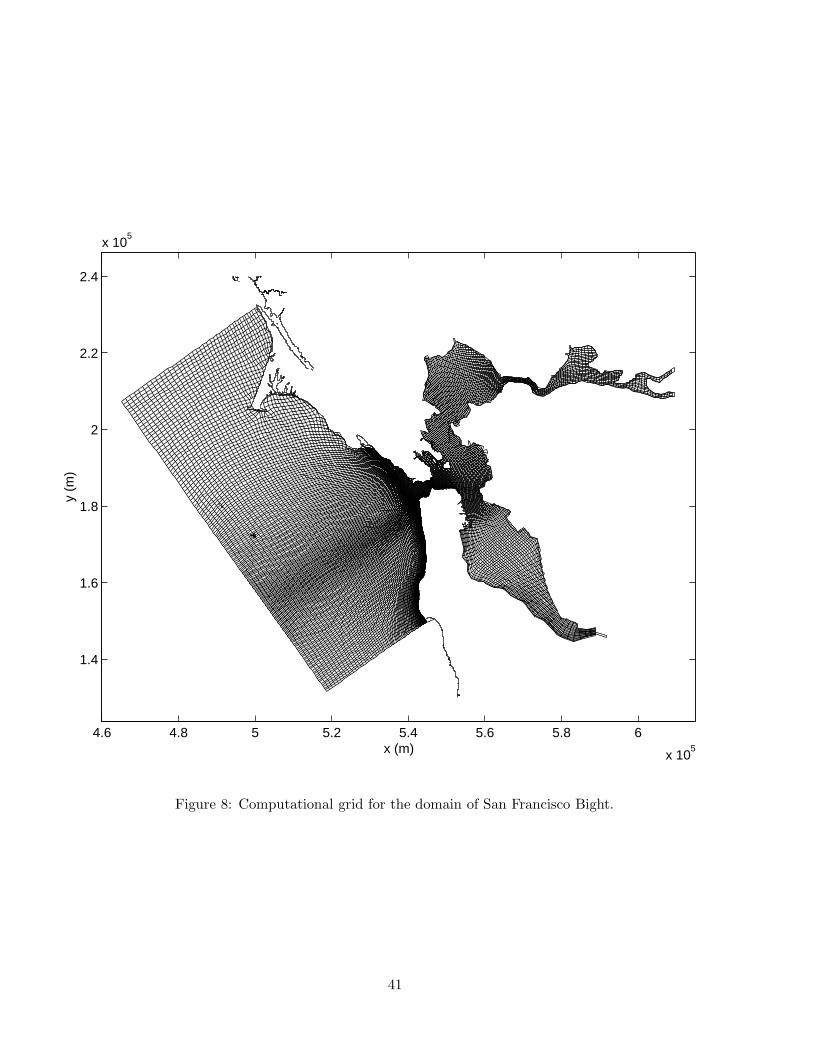
4.6 4.8 5 5.2 5.4 5.6 5.8 6

x 105

1.4

1.6

1.8

2

2.2

2.4

x 105

x (m)

y (m

)

Figure 8: Computational grid for the domain of San Francisco Bight.

41

5.32 5.34 5.36 5.38 5.4 5.42 5.44 5.46 5.48 5.5

x 105

1.76

1.78

1.8

1.82

1.84

1.86

1.88

x 105

x (m)

y (m

)

Figure 9: Blow-up of the computational grid at the inlet and Ocean Beach.

5.34 5.36 5.38 5.4 5.42 5.44 5.46 5.48

x 105

1.74

1.76

1.78

1.8

1.82

1.84

1.86

1.88x 10

5

15

12 8

1215

15

20

25

12

12

15

2025

30

40

50 40

50

5070

110

15

12

15

8

42

8

O

SITE

x(m)

y(m

)

OceanBeach

Baker Beach

Marin Headlands

Figure 10: Nearshore bathymetry and the measurement location (SITE)

42

73 74 75 76 77 78 79 80 810

0.5

1

1.5

2

time (yearday of 1998)

surf

ace

elev

atio

n (m

)

dataCr=10Cr = 100

Figure 11: Model/data comparison of surface elevations at a location (SITE) near

the Golden Gate channel.

43

73 74 75 76 77 78 79 80 81−0.2

0

0.2

0.4

0.6

0.8

1

1.2

1.4

1.6

1.8

time (yearday of 1998)

ampl

itude

of d

epth

−av

erag

ed v

eloc

ity (

m/s

)

dataCr=10Cr=100

Figure 12: Model/data comparison of depth-averaged tidal current magnitude at a

location (SITE) near the Golden Gate channel.

44

5.4 5.41 5.42 5.43 5.44 5.45 5.46

x 105

1.72

1.74

1.76

1.78

1.8

1.82

1.84

1.86

x 105

x (m)

y (m

)

2.0 m/s

Figure 13: Snapshot of tidal current field during flood tide

45

5.4 5.41 5.42 5.43 5.44 5.45 5.46

x 105

1.72

1.74

1.76

1.78

1.8

1.82

1.84

1.86

x 105

x (m)

y (m

)

2.0 m/s

Figure 14: Snapshot of tidal current field during ebb tide

46

5.4 5.41 5.42 5.43 5.44

x 105

1.72

1.74

1.76

1.78

1.8

1.82

1.84x 10

5

x (m)

y (m

)

1.0 m/s

Figure 15: Wave-induced longshore currents under incident wave conditions of 3m

significant wave height, and 15 seconds peak period in deep water, and 10m/s wind

from 300◦ over the whole domain.

47