AN AUTONOMOUS GPS-DENIED UNMANNED VEHICLE …
7
AN AUTONOMOUS GPS-DENIED UNMANNED VEHICLE PLATFORM BASED ON BINOCULAR VISION FOR PLANETARY EXPLORATION Man Qin 1,2,* , Xue Wan 1,2 , Yu-Yang Shao 1,2 , Sheng-Yang Li 1,2 1 Technology and Engineering Center for Space Utilization, Chinese Academy of Sciences, Beijing, China - (shyli, wanxue, shaoyy, qinman)@ csu.ac.cn 2 Key Laboratory of Space Utilization, Chinese Academy of Sciences, Beijing, China - (shyli, wanxue, shaoyy, qinman)@ csu.ac.cn KEY WORDS: Planetary Exploration, Unmanned Vehicle Platform, Vision-based Navigation, Feature Matching, 3D Reconstruction ABSTRACT: Vision-based navigation has become an attractive solution for autonomous navigation for planetary exploration. This paper presents our work of designing and building an autonomous vision-based GPS-denied unmanned vehicle and developing an ARFM (Adaptive Robust Feature Matching) based VO (Visual Odometry) software for its autonomous navigation. The hardware system is mainly composed of binocular stereo camera, a pan-and tilt, a master machine, a tracked chassis. And the ARFM-based VO software system contains four modules: camera calibration, ARFM-based 3D reconstruction, position and attitude calculation, BA (Bundle Adjustment) modules. Two VO experiments were carried out using both outdoor images from open dataset and indoor images captured by our vehicle, the results demonstrate that our vision-based unmanned vehicle is able to achieve autonomous localization and has the potential for future planetary exploration. 1. INTRODUCTION Accurate and autonomous localization of spacecraft and rover is essential for planetary exploration. Traditional navigation method based on ground remote control system cannot achieve autonomous navigation in terms of communication latency and bandwidth limitation. While autonomous navigation can be achieved by GPS on Earth, there is no such positioning system on other planets. The optical camera has the characteristics of low cost, wide application range, low power consumption and large field of view compared with the other detection devices, thus vision-based navigation has become an attractive solution for autonomous navigation. The combination of unmanned vehicle platform and robust computer vision algorithms is a challenge task. In this paper, a binocular camera based unmanned vehicle platform has been built and an ARFM (Adaptive Robust Feature Matching) based VO (Visual Odometry) software system has been developed to achieve GPS-denied autonomous navigation for planetary exploration. 2. RELATED WORK In 2004, NASA has launched Spirit and Opportunity (Cheng Y et al., 2006), after that, the Mars Science Laboratory (MSL) team has launched the Curiosity rover (Sumner D, 2013) in August 2012. In 2013, China has launched Yutu (Zhou J et al., 2014), which has accomplished the exploration mission until 2016. ESA will launch Exo Mars (Griffiths A D et al., 2006) in the near future. Vision-based navigation had been used for planetary exploration in these unmanned vehicles, which proved successfully. However, vision-based navigation for planetary rover has the following challenges: 1) The images taken may contain scale and rotation distortions; 2) The real-time and accuracy requirement must be met; 3) There are some featureless areas which may decrease the feature matching accuracy. Thus, the matching result of traditional feature extraction algorithms, such as Harris (Stephens M, 1988), Shi-Tomasi, Susan corner detection algorithm and SIFT (Scale Invariant Feature Transform) (David G. Lowe, 2004), are unsatisfied. Thus, real-time, accuracy and reliability must be taken into consideration, not only in hardware but also in software. 3. THE BINOCULAR VISION BASED AUTONOMOUS UNMANNED VEHICLE In this paper, an unmanned vehicle platform based on binocular vision has been designed and built. We also developed an ARFM-based VO software for its autonomous navigation. This section will present our work in terms of both hardware system and the software system. The unmanned vehicle platform can navigate by the ARFM- based VO software automatically in the process of walking, but manually stop or start is needed. 3.1 The hardware system The unmanned vehicle we designed is a ground mobile robot with three independent hierarchical layers, as is shown in Fig. 1. The upper layer is made up of a binocular camera and a pan-and-tilt, which is used to receive the image sequence and precisely control the attitude of the camera. The middle layer is a master machine for processing the image streams transferred from the upper and issuing instructions, for example, moving forward or backward. The lower layer is a tracked chassis which can drive this unmanned vehicle according to the instructions received form the middle. The maximum speed is set to 0.1m/s because of the rough surface of planetary. Fig. 1 The unmanned vehicle with three independent hierarchical layers The International Archives of the Photogrammetry, Remote Sensing and Spatial Information Sciences, Volume XLII-3, 2018 ISPRS TC III Mid-term Symposium “Developments, Technologies and Applications in Remote Sensing”, 7–10 May, Beijing, China This contribution has been peer-reviewed. https://doi.org/10.5194/isprs-archives-XLII-3-1439-2018 | © Authors 2018. CC BY 4.0 License. 1439
Transcript of AN AUTONOMOUS GPS-DENIED UNMANNED VEHICLE …

AN AUTONOMOUS GPS-DENIED UNMANNED VEHICLE PLATFORM BASED ON
BINOCULAR VISION FOR PLANETARY EXPLORATION
Man Qin 1,2,* , Xue Wan 1,2, Yu-Yang Shao1,2, Sheng-Yang Li 1,2
1 Technology and Engineering Center for Space Utilization, Chinese Academy of Sciences, Beijing, China - (shyli, wanxue, shaoyy,
qinman)@ csu.ac.cn 2 Key Laboratory of Space Utilization, Chinese Academy of Sciences, Beijing, China - (shyli, wanxue, shaoyy, qinman)@ csu.ac.cn
KEY WORDS: Planetary Exploration, Unmanned Vehicle Platform, Vision-based Navigation, Feature Matching, 3D Reconstruction
ABSTRACT:
Vision-based navigation has become an attractive solution for autonomous navigation for planetary exploration. This paper presents
our work of designing and building an autonomous vision-based GPS-denied unmanned vehicle and developing an ARFM (Adaptive
Robust Feature Matching) based VO (Visual Odometry) software for its autonomous navigation. The hardware system is mainly
composed of binocular stereo camera, a pan-and tilt, a master machine, a tracked chassis. And the ARFM-based VO software system
contains four modules: camera calibration, ARFM-based 3D reconstruction, position and attitude calculation, BA (Bundle Adjustment)
modules. Two VO experiments were carried out using both outdoor images from open dataset and indoor images captured by our
vehicle, the results demonstrate that our vision-based unmanned vehicle is able to achieve autonomous localization and has the potential
for future planetary exploration.
1. INTRODUCTION
Accurate and autonomous localization of spacecraft and rover is
essential for planetary exploration. Traditional navigation
method based on ground remote control system cannot achieve
autonomous navigation in terms of communication latency and
bandwidth limitation. While autonomous navigation can be
achieved by GPS on Earth, there is no such positioning system
on other planets. The optical camera has the characteristics of low
cost, wide application range, low power consumption and large
field of view compared with the other detection devices, thus
vision-based navigation has become an attractive solution for
autonomous navigation. The combination of unmanned vehicle
platform and robust computer vision algorithms is a challenge
task. In this paper, a binocular camera based unmanned vehicle
platform has been built and an ARFM (Adaptive Robust Feature
Matching) based VO (Visual Odometry) software system has
been developed to achieve GPS-denied autonomous navigation
for planetary exploration.
2. RELATED WORK
In 2004, NASA has launched Spirit and Opportunity (Cheng Y
et al., 2006), after that, the Mars Science Laboratory (MSL) team
has launched the Curiosity rover (Sumner D, 2013) in August
2012. In 2013, China has launched Yutu (Zhou J et al., 2014),
which has accomplished the exploration mission until 2016. ESA
will launch Exo Mars (Griffiths A D et al., 2006) in the near
future. Vision-based navigation had been used for planetary
exploration in these unmanned vehicles, which proved
successfully. However, vision-based navigation for planetary
rover has the following challenges: 1) The images taken may
contain scale and rotation distortions; 2) The real-time and
accuracy requirement must be met; 3) There are some featureless
areas which may decrease the feature matching accuracy. Thus,
the matching result of traditional feature extraction algorithms,
such as Harris (Stephens M, 1988), Shi-Tomasi, Susan corner
detection algorithm and SIFT (Scale Invariant Feature Transform)
(David G. Lowe, 2004), are unsatisfied. Thus, real-time, accuracy
and reliability must be taken into consideration, not only in
hardware but also in software.
3. THE BINOCULAR VISION BASED AUTONOMOUS
UNMANNED VEHICLE
In this paper, an unmanned vehicle platform based on binocular
vision has been designed and built. We also developed an
ARFM-based VO software for its autonomous navigation. This
section will present our work in terms of both hardware system
and the software system.
The unmanned vehicle platform can navigate by the ARFM-
based VO software automatically in the process of walking, but
manually stop or start is needed.
3.1 The hardware system
The unmanned vehicle we designed is a ground mobile robot with
three independent hierarchical layers, as is shown in Fig. 1. The
upper layer is made up of a binocular camera and a pan-and-tilt,
which is used to receive the image sequence and precisely control
the attitude of the camera. The middle layer is a master machine
for processing the image streams transferred from the upper and
issuing instructions, for example, moving forward or backward.
The lower layer is a tracked chassis which can drive this
unmanned vehicle according to the instructions received form the
middle. The maximum speed is set to 0.1m/s because of the rough
surface of planetary.
Fig. 1 The unmanned vehicle with three independent
hierarchical layers
The International Archives of the Photogrammetry, Remote Sensing and Spatial Information Sciences, Volume XLII-3, 2018 ISPRS TC III Mid-term Symposium “Developments, Technologies and Applications in Remote Sensing”, 7–10 May, Beijing, China
This contribution has been peer-reviewed. https://doi.org/10.5194/isprs-archives-XLII-3-1439-2018 | © Authors 2018. CC BY 4.0 License.
1439

3.2 The ARFM-based VO software system
The software system contains four modules: camera calibration,
ARFM-based 3D reconstruction, position and attitude calculation,
BA (Bundle Adjustment) modules. Fig. 2 shows the workflow of
the VO software system.
Camera Calibration
Module
Parameters
ARFM-based 3D Reconstruction
Module
POsition and Attitude
Calculation Module
BA module
SURF+FLANN AT
PNP
Image Sequence
Fig. 2 The workflow of the ARFM-based VO software system.
3.2.1 Camera Calibration Module: Camera calibration is a
necessary step in 3D reconstruction in order to extract metric
information from 2D images. This paper performs the calibration
of binocular stereo measuring system reliably by Zhang’s
algorithm (Zhang Z, 2002), and gets the extrinsic and intrinsic
parameters. In Zhang’s algorithm, a 2D point is denoted by [𝑥 𝑦]𝑇, and a 3D point is denoted by [𝑋 𝑌 𝑍]𝑇. A camera is
modeled by the usual pinhole: the relationship between a 3D
point and its image projection is given by
𝑠 [𝑥𝑦1] = 𝐴[𝑅 𝑡] [
𝑋𝑌𝑍1
],with A = [
𝛼 𝑐 𝑢00 𝛽 𝑣00 0 1
] (1)
where 𝑠 is an arbitrary scale factor; [𝑅 𝑡], called the extrinsic
parameters, is the rotation and translation which relates the world
coordinate system to the camera coordinate system; A is called
the camera intrinsic matrix, and (𝑢0 𝑣0) are the coordinates of
the principal point, α and β the scale factors in image 𝑢 and 𝑣
axes, and 𝑐 the parameter describing the skewness of the two
image axes.
3.2.2 ARFM-based 3D Reconstruction Module: In this
paper, we propose an ARFM algorithm to guarantee the accuracy
and reliability, and adapt to the changed of environment as well.
In this algorithm. We use SURF (Speed-up Robust Features)
(Bay et al., 2008) to find point correspondences between two
images. In order to reduce the computational cost, SURF takes
the integral image, which represents the sum of all pixels in the
input image I within a rectangular region formed by the origin
and x. The integral image 𝐼Σ(x) at [𝑥 𝑦]𝑇 is
𝐼Σ(x) = ∑ ∑ 𝐼(𝑖, 𝑗)𝑗≤𝑦𝑗=0
𝑖≤𝑥𝑖=0 (2)
The Hessian-based detectors are scale-invariant, moreover, are
more stable and repeatable than their Harris-based counterparts,
so Hessian is used to detect feature points.
Given a point x = (x, y) in an image I , the Hessian matrix
Η(x, σ) in x at scale σ is defined as follows
Η(x, σ) = [𝐿𝑥𝑥(x, σ) 𝐿𝑥𝑦(x, σ)
𝐿𝑥𝑦(x, σ) 𝐿𝑦𝑦(x, σ)] (3)
where 𝐿𝑥𝑥(x, σ) is the convolution of the Gaussian second order
derivative 𝜕2
𝜕𝑥2𝑔(𝜎) with the image I in point x, and similarly for
𝐿𝑥𝑦(x, σ) and 𝐿𝑦𝑦(x, σ).
SURF used box filter to guarantee scale-invariance and integral
image to avoid iterative calculation, so it can extract feature
points quickly. According to the neighbourhood of these points,
descriptors which are robust to noise, detection displacements
and geometric and photometric deformations, are generated. The
descriptor is similar to the gradient information extracted by
SIFT, but use only 64 dimensions, which reduces the time for
feature computation. After that, the descriptor vectors between
different images is matched based on Euclidean distance.
But SURF is high error matching, so optimized bothway FLANN
(Fast Library for Approximate Nearest Neighbors) (M Muja et
al., 2009) is used to match SURF descriptor. Given a set points
P = {𝑝1, … , 𝑝𝑛} which is extracted from left image and Q ={𝑞1, … , 𝑞𝑛} which is extracted from right image, and dist(𝑝𝑖 , 𝑞𝑗)
which is the Euclidean distance from 𝑝𝑖 to 𝑞𝑗. Then the nearest
neighbour dist(𝑝𝑖 , 𝑞𝑗) and the second-nearest neighbour
dist(𝑝𝑖 , 𝑞𝑘) can be calculated. dist(𝑝𝑖 , 𝑞𝑗) is the optimal value if
dist(𝑝𝑖 , 𝑞𝑗) is far less than dist(𝑝𝑖 , 𝑞𝑘) so that (𝑝𝑖 , 𝑞𝑗) is a pair
of matching points. However, if dist(𝑝𝑖 , 𝑞𝑗) is similar to
dist(𝑝𝑖 , 𝑞𝑘) , 𝑞𝑗 and 𝑞𝑘 is too similar to decide who is the
matching point to 𝑝𝑖, so both points must be abandoned. Only in
the condition of (𝑝𝑖 , 𝑞𝑗) and (𝑞𝑗 , 𝑝𝑖) is the same can be matched.
In order to guarantee precision, RANSAC is used to eliminate the
mismatched feature points. In this way, the accuracy and
reliability requirement can be met. Meanwhile, scale and rotation
distortions can be overcame.
Traditional matching method uses a FT (fixed Threshold)
algorithm. To adapt the environment variation, we proposed an
AT (Adaptive Threshold) algorithm that can automatically adjust
the threshold according to the variances of image.
Gray =∑ ∑ 𝐺(𝑖, 𝑗)𝑁
𝑗=1𝑀𝑖=1
𝑀 ×𝑁 (4)
𝜎2 =∑ ∑ [𝐺(𝑖, 𝑗) − Gray]2𝑁
𝑗=1𝑀𝑖=1
𝑀 ×𝑁 (5)
where G(𝑖, 𝑗) are the gray values of current image and Gray is the
average gray value of current image, 𝑀 and 𝑁 are the height and
width of current image. 𝜎2 is the variances of current image,
which can be used to adjust the threshold automatically. And then
the 3D point cloud is generated using the calibration and the
feature matching results. The focus length of camera is denoted
by 𝑓, and the baseline is denoted by 𝑇. The value of parallax is
denoted by disp. So the depth of 3D point is calculated by
𝑍 = 𝑇𝑓
disp (6)
The International Archives of the Photogrammetry, Remote Sensing and Spatial Information Sciences, Volume XLII-3, 2018 ISPRS TC III Mid-term Symposium “Developments, Technologies and Applications in Remote Sensing”, 7–10 May, Beijing, China
This contribution has been peer-reviewed. https://doi.org/10.5194/isprs-archives-XLII-3-1439-2018 | © Authors 2018. CC BY 4.0 License.
1440
3.2.3 Position and Attitude Calculation Module: In this
module, the current pose of camera is computed according to the
3D point cloud generated from 3D reconstruction module and the
current 2D image projection point based on a PNP (Perspective-
N-Point) (Fischler et al., 1981) algorithm. To reduce the
accumulative error, this paper uses 3D points within the FOV
(Field of View) from all relevant images to build a local map. As
is seen in Fig. 3, the straight lines represent the 3D reconstruction,
thus the 3D coordinates can be calculated, and the dotted lines
represent the 2D image point projected on current position.
3D points within the FOV
Current Position
Local Map
Previous Position
Fig. 3 The principle of position and attitude calculation using
local map.
PNP is as follow:
First of all, original R and t are calculated from 4 points according
to perspective projection model, and the image coordinates
𝐶𝑗𝑐 , 𝑗 = 1,2,3,4 are calculated according to.
{
∑𝛼𝑖𝑗[𝑓𝑥𝑋𝑗
𝑐 + 𝑍𝑗𝑐(𝑐𝑥 − 𝑢𝑖)] = 0
4
𝑗=1
∑𝛼𝑖𝑗[𝑓𝑥𝑌𝑗𝑐 + 𝑍𝑗
𝑐(𝑐𝑦 − 𝑣𝑖)] = 0
4
𝑗=1
(7)
Then, minimize
Error(𝛽) = ∑ |‖𝐶𝑖𝑐 − 𝐶𝑗
𝑐‖2− ‖𝐶𝑖
𝑤 − 𝐶𝑗𝑤‖
2|4
𝑖,𝑗=1,𝑖<𝑗 (8)
with the other points according to Gauss-Newton algorithm, thus
take 𝐶𝑗𝑐 , j = 1,2,3,4 and 𝑃𝑖
𝑐 . Finally, R and t can be obtained
from 𝑃𝑖𝑐.
3.2.4 BA Module: BA imposes geometrical constraints over
multiple frames, thus providing a global optimal estimate by
minimizing the re-projection errors. In this study, global BA
(Eudes et al., 2010), which takes the 3D point clouds and all
camera poses together at once, is used. The positions of
unmanned vehicle and 3D point clouds, including rotation vector
and translation vector. And the relationship between positions are
noted as edges to build graph. The re-projection errors can be
minimized by LM (Levenberg-Marquardt) (Marquardt, 1963)
and Gauss-Newton algorithm. The principle of BA is shown in
Figure 4.
CP1 CP2 CP3
PC1PC2 PC3
CP4
PC4
Fig. 4 The principle of BA.
4. EXPERIMENT
In this study, the performance of the matching algorithm and the
ARFM-based VO software system are tested. First, an algorithm
experiment is performed, which proved ARFM is useful to
improve the matching precision. Then, two experiments have
been conducted to test the VO software. Our platform is tested by
the indoors image sequence captured by binocular camera
equipped on our platform using internal and external parameters,
which are approached by calibration. In the other experiment, the
ARFM-based VO software system is tested using an open dataset:
KITTI, which are outdoors image sequence captured by
binocular camera equipped on moving cars.
4.1 Experiments
This experiment section is made up of two parts: the comparison
results of matching using our adaptive threshold method: AT and
the traditional fixed threshold method: FT, the comparison of
different matching strategies.
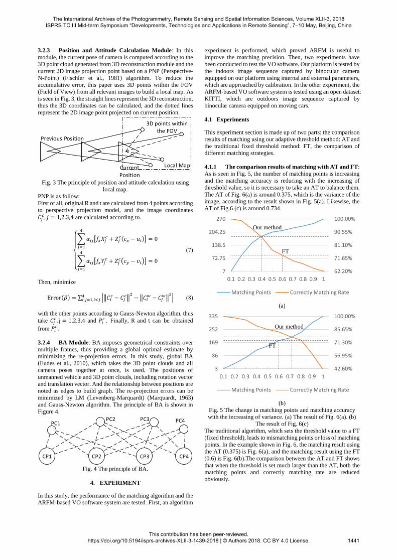
4.1.1 The comparison results of matching with AT and FT:
As is seen in Fig. 5, the number of matching points is increasing
and the matching accuracy is reducing with the increasing of
threshold value, so it is necessary to take an AT to balance them.
The AT of Fig. 6(a) is around 0.375, which is the variance of the
image, according to the result shown in Fig. 5(a). Likewise, the
AT of Fig.6 (c) is around 0.734.
(a)
(b)
Fig. 5 The change in matching points and matching accuracy
with the increasing of variance. (a) The result of Fig. 6(a). (b)
The result of Fig. 6(c)
The traditional algorithm, which sets the threshold value to a FT
(fixed threshold), leads to mismatching points or loss of matching
points. In the example shown in Fig. 6, the matching result using
the AT (0.375) is Fig. 6(a), and the matching result using the FT
(0.6) is Fig. 6(b).The comparison between the AT and FT shows
that when the threshold is set much larger than the AT, both the
matching points and correctly matching rate are reduced
obviously.
62.20%
71.65%
81.10%
90.55%
100.00%
7
72.75
138.5
204.25
270
0.1 0.2 0.3 0.4 0.5 0.6 0.7 0.8 0.9 1
Matching Points Correctly Matching Rate
42.60%
56.95%
71.30%
85.65%
100.00%
3
86
169
252
335
0.1 0.2 0.3 0.4 0.5 0.6 0.7 0.8 0.9 1
Matching Points Correctly Matching Rate
Our method
FT
FT
Our method
The International Archives of the Photogrammetry, Remote Sensing and Spatial Information Sciences, Volume XLII-3, 2018 ISPRS TC III Mid-term Symposium “Developments, Technologies and Applications in Remote Sensing”, 7–10 May, Beijing, China
This contribution has been peer-reviewed. https://doi.org/10.5194/isprs-archives-XLII-3-1439-2018 | © Authors 2018. CC BY 4.0 License.
1441

(a)Our method(AT)
(b)Traditional method(FT)
Fig. 6 The comparison between using the AT and the larger
FT. (a) Matching result with AT = 0.375, the number of
matching points is 175 and the correctly matching rate is
87.02%. (b) Matching result with FT =0.6, the number of
matching points is 83 and the correctly matching rate is
74.28%.
In the example shown in Fig. 7, the adaptive threshold is larger
compared with the value in Fig. 6. And the matching result
using the adaptive threshold (0.734) is Fig. 7(a), the matching
result using the fixed threshold (0.6) is Fig. 7(b).The
comparison between the adaptive threshold and fixed
threshold shows that when the threshold is set much smaller
than the adaptive, the number of correctly matching points is
less.
(a)Our method(AT)
(b)Traditional method(FT)
Fig. 7 The comparison between using the AT and the
smaller FT. (a) Matching result with AT = 0.734, the
number of matching points is 212 and the correctly matching
rate is 78.24%. (b) Matching result with FT =0.6, the number
of matching points is 172 and the correctly matching rate is
71.9%. So, we can draw the conclusion that taking the variance, which is
calculated according to the image, as threshold value, contributes
to guarantee the maximization of both the matching points and
matching accuracy, and set the threshold value as variance of
image dynamically is necessary.
4.1.2 The comparison of different matching strategies: As
discussed, ARFM is made up of SURF, FLANN, AT and
RANSAC. The matching result of four strategies is shown in Fig.
8, and the statistics is shown in Fig. 9. The number of matching
points and correctly matching points is reduced, but the matching
rate is increasing with four strategies: SURF, SURF+RANSAC,
SURF+FLANN, SURF+FLANN+RANSAC, so ARFM has the
highest matching accuracy in these methods.
(a) Matching result of SURF
(b) Matching result of SURF+RANSAC
(c) Matching result of SURF+FLANN
(d) Matching result of SURF+FLANN+RANSAC
Fig. 8 The matching result using four strategies.
Fig. 9 The statistics of matching result with four strategies.
59.40%71.90%
77.30% 78.40%
0.00%
16.67%
33.33%
50.00%
66.67%
83.33%
100.00%
0
100
200
300
400
500
600
SURF SURF+RANSAC
SURF+FLANN
SURF+FLANN
+RANSAC
Matching Points
Correctly Matching Points
Correctly Matching Rate
The International Archives of the Photogrammetry, Remote Sensing and Spatial Information Sciences, Volume XLII-3, 2018 ISPRS TC III Mid-term Symposium “Developments, Technologies and Applications in Remote Sensing”, 7–10 May, Beijing, China
This contribution has been peer-reviewed. https://doi.org/10.5194/isprs-archives-XLII-3-1439-2018 | © Authors 2018. CC BY 4.0 License.
1442

Fig. 10 shows the trajectories of four statistics and ground truth,
and Fig. 11 shows the translation error and run time of four
strategies. From the comparison, we observe that SURF is the
worst algorithm not only in translation error but also in run time.
SURF+FLANN is of higher precision relativity, while the speed
is the highest. The run time of SURF+RANSAC and
SURF+FLANN+RANSAC is similar, but the precision of
SURF+FLANN+RANSAC is higher. So, if the precision is the
most important, SURF+FLANN+RANSAC is the best choice,
and if the run time is the most important, SURT+FLANN is the
best choice.
Fig. 10 The trajectories of four methods and ground truth.
Fig. 11 The translation error and run time of four methods.
4.2 Indoor VO Experiment
In this experiment, a specifically designed calibration board is
made to calibrate. The board is full of black and white squares
whose size is 210×110cm. Each square is 10×10cm so that the
calibration board has 20×10 corners. By using the unmanned
vehicle we built, 63 pairs of stereo calibration images were
collected, which are shown in Fig.12, and the results of
calibration are showed in Fig.13. Fig. 13(a) is a corner detection
of the calibration board. Fig. 13(b) shows a rectified result.
Meanwhile, internal and external parameters of each camera is
obtained.
(a)
(b)
(c)
(d)
(e)
(f)
Fig. 12 Images of the calibration board
(a) Corner detection.
(b) A rectified result.
Fig. 13 The result of stereo calibration.
Then, we tested our platform indoors on 16 December. 2017. In
this experiment, an image sequence of 6 pairs with 1624×1234
resolution was captured. Some of the images are shown in Fig.
14. The experimental results are shown in Fig. 15.
(a)
(b)
(c)
(d)
-0.2 -0.1 0 0.1 0.2 0.3 0.4 0.5 0.6 0.7 0.80
1
2
3
4
5
6
7
8
9
10
11
x [m]
z [
m]
Ground Truth
VO(SURF)
VO(SURF+FLANN)
VO(SURF+RANSAC)
VO(SURF+FLANN+RANSAC)
Sequence Start
0
50
100
150
200
00.0005
0.0010.0015
0.0020.0025
0.0030.0035
0.004
SURF SURF+FLANN
SURF+RANSAC
SURF+FLANN
+RANSACTranslation error(m/10m)
Run Time(s/frame)
The International Archives of the Photogrammetry, Remote Sensing and Spatial Information Sciences, Volume XLII-3, 2018 ISPRS TC III Mid-term Symposium “Developments, Technologies and Applications in Remote Sensing”, 7–10 May, Beijing, China
This contribution has been peer-reviewed. https://doi.org/10.5194/isprs-archives-XLII-3-1439-2018 | © Authors 2018. CC BY 4.0 License.
1443
(e)
(f)
Fig. 14 Images the unmanned vehicle captured to perform the
first experiment.
Fig. 15 The result of ARMF-base VO system using the images
we captured. In this coordinates, the blue line represents the
path calculated by the ARMF-base VO system, and the black
point represents the start position.
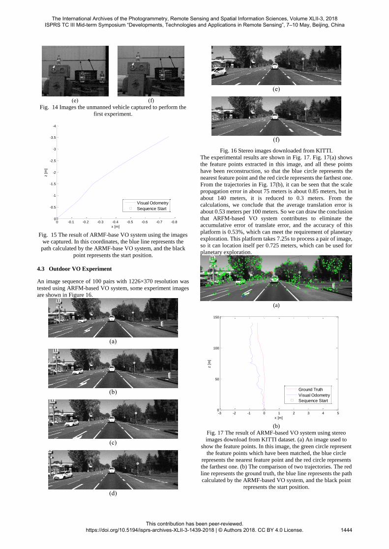
4.3 Outdoor VO Experiment
An image sequence of 100 pairs with 1226×370 resolution was
tested using ARFM-based VO system, some experiment images
are shown in Figure 16.
(a)
(b)
(c)
(d)
(e)
(f)
Fig. 16 Stereo images downloaded from KITTI. The experimental results are shown in Fig. 17. Fig. 17(a) shows
the feature points extracted in this image, and all these points
have been reconstruction, so that the blue circle represents the
nearest feature point and the red circle represents the farthest one.
From the trajectories in Fig. 17(b), it can be seen that the scale
propagation error in about 75 meters is about 0.85 meters, but in
about 140 meters, it is reduced to 0.3 meters. From the
calculations, we conclude that the average translation error is
about 0.53 meters per 100 meters. So we can draw the conclusion
that ARFM-based VO system contributes to eliminate the
accumulative error of translate error, and the accuracy of this
platform is 0.53%, which can meet the requirement of planetary
exploration. This platform takes 7.25s to process a pair of image,
so it can location itself per 0.725 meters, which can be used for
planetary exploration.
(a)
(b)
Fig. 17 The result of ARMF-based VO system using stereo
images download from KITTI dataset. (a) An image used to
show the feature points. In this image, the green circle represent
the feature points which have been matched, the blue circle
represents the nearest feature point and the red circle represents
the farthest one. (b) The comparison of two trajectories. The red
line represents the ground truth, the blue line represents the path
calculated by the ARMF-based VO system, and the black point
represents the start position.
-0.8-0.7-0.6-0.5-0.4-0.3-0.2-0.10
-4
-3.5
-3
-2.5
-2
-1.5
-1
-0.5
0
x [m]
z [
m]
Visual Odometry
Sequence Start
-3 -2 -1 0 1 2 3 4 50
50
100
150
x [m]
z [
m]
Ground Truth
Visual Odometry
Sequence Start
The International Archives of the Photogrammetry, Remote Sensing and Spatial Information Sciences, Volume XLII-3, 2018 ISPRS TC III Mid-term Symposium “Developments, Technologies and Applications in Remote Sensing”, 7–10 May, Beijing, China
This contribution has been peer-reviewed. https://doi.org/10.5194/isprs-archives-XLII-3-1439-2018 | © Authors 2018. CC BY 4.0 License.
1444

5. CONCLUSION
In this paper, an autonomous GPS-denied unmanned vehicle
platform based on binocular vision has been designed and built
for planetary exploration. An ARMF-base VO system containing
four modules, has been developed to achieve vision-based GPS-
denied autonomous navigation. The algorithm experiment proves
that our ARMF is the best choice applied to our unmanned
vehicle. Then, experiments using both outdoor images from open
dataset and indoor images captured by our vehicle demonstrate
that our unmanned vehicle, which combined both hardware and
software system, is able to achieve autonomous localization and
has the potential for future planetary exploration.
REFERENCES
Cheng Y, Maimone M, Matthies L. Visual odometry on the Mars
Exploration Rovers[C]// IEEE International Conference on
Systems, Man and Cybernetics. IEEE, 2006:903-910 Vol. 1.
Sumner D, Mars Science Laboratory Team. Curiosity on Mars:
The Latest Results from an Amazing Mission[C]// American
Astronomical Society Meeting. American Astronomical Society
Meeting Abstracts, 2013.
Zhou J, Xie Y, Zhang Q, et al. Research on mission planning in
teleoperation of lunar rovers[J]. Scientia Sinica, 2014, 44(4):441.
Griffiths A D, Coates A J, Jaumann R, et al. Context for the ESA
ExoMars rover: the Panoramic Camera (PanCam) instrument[J].
International Journal of Astrobiology, 2006, 5(3):269-275.
Stephens M. A Combined Comer and Edge Detector[J]. 1988.
Eudes A, Naudet-Collette S, Lhuillier M, et al. Weighted Local
Bundle Adjustment and Application to Odometry and Visual
SLAM Fusion[C]// British Machine Vision Conference, BMVC
2010, Aberystwyth, UK, August 31 - September 3, 2010.
Proceedings. DBLP, 2010:1-10.
Lowe D G. Object Recognition from Local Scale-Invariant
Features[C]// Proc. IEEE International Conference on Computer
Vision. 1999:1150.
Zhang Z. Flexible Camera Calibration by Viewing a Plane from
Unknown Orientations[C]// The Proceedings of the Seventh
IEEE International Conference on Computer Vision. IEEE,
2002:666-673 vol.1.
Bay H, Ess A, Tuytelaars T, et al. Speeded-Up Robust Features
(SURF)[J]. Computer Vision & Image Understanding, 2008,
110(3):346-359.
Muja M. FLANN -Fast Library for Approximate Nearest
Neighbors User Manual[J]. 2009.
Bolles R C, Fischler M A. RANSAC-BASED APPROACH TO
MODEL FITTING AND ITS APPLICATION TO FINDING
CYLINDERS IN RANGE DATA[C]// International Joint
Conference on Artificial Intelligence. 1981.
Fischler M A, Bolles R C. Random sample consensus: a
paradigm for model fitting with applications to image analysis
and automated cartography[M]. ACM, 1981.
The International Archives of the Photogrammetry, Remote Sensing and Spatial Information Sciences, Volume XLII-3, 2018 ISPRS TC III Mid-term Symposium “Developments, Technologies and Applications in Remote Sensing”, 7–10 May, Beijing, China
This contribution has been peer-reviewed. https://doi.org/10.5194/isprs-archives-XLII-3-1439-2018 | © Authors 2018. CC BY 4.0 License.
1445