An automatic approach to the detection and extraction of...

90 IEEE JOURNAL OF OCEANIC ENGINEERING, VOL. 28, NO. 1, JANUARY 2003

An Automatic Approach to the Detection andExtraction of Mine Features in Sidescan Sonar

Scott Reed, Yvan Petillot, and Judith Bell

Abstract—Mine detection and classification using high-reso-lution sidescan sonar is a critical technology for mine countermeasures (MCM). As opposed to the majority of techniques whichrequire large training data sets, this paper presents unsupervisedmodels for both the detection and the shadow extraction phases ofan automated classification system. The detection phase is carriedout using an unsupervised Markov random field (MRF) modelwhere the required model parameters are estimated from theoriginal image. Usinga priori spatial information on the physicalsize and geometric signature of mines in sidescan sonar, a detec-tion-orientated MRF model is developed which directly segmentsthe image into regions of shadow, seabottom-reverberation, andobject-highlight. After detection, features are extracted so thatthe object can be classified. A novel co-operating statistical snake(CSS) model is presented which extracts the highlight and shadowof the object. The CSS model again utilizes availablea prioriinformation on the spatial relationship between the highlight andshadow, allowing accurate segmentation of the object’s shadowto be achieved on a wide range of seabed types. Results are givenfor both models on real and synthetic images and are shown tocompare favorably with other models in this field.

Index Terms—A priori information, automated mine detection,image analysis, Markov random field (MRF) models, shadow ex-traction, statistical snakes.

I. INTRODUCTION

T HE ANALYSIS of sidescan sonar images in the field ofmine countermeasures (MCM) is traditionally carried out

by a skilled human operator. This analysis is difficult due to thelarge variability in the appearance of the sidescan images as wellas the high levels of noise usually present in the images. With theadvances in autonomous underwater vehicle (AUV) technology,automated techniques are now required to replace the operatorto carry out this analysis on-board.

Complete MCM systems are usually composed of a detectionand a classification process such as the systems by Dobecket al. [1], Ciany et al. [2], [3], and Aridgideset al. [4]. Allthree of these systems operate using the detection/classificationframework although they operate using very different models.Dobeck implements a matched filter in [1] to detect mine-likeobjects (MLOs) after which both a -nearest neighbor neuralnetwork classifier and a discriminatory filter classifier areused to classify the objects as mine or not-mine. The detectionprocess is relatively simple and is primarily for identifyingregions which definitely do not contain MLOs. The classifi-

Manuscript received April 22, 2002; revised August 23, 2002.The authors are with the Ocean Systems Laboratory, Department of

Computing and Electrical Engineering, Heriot-Watt University, Riccarton,Edinburgh EH14 4AS, U.K.

Digital Object Identifier 10.1109/JOE.2002.808199

cation process then uses up to 45 features for every possibleMLO to determine which are real MLOs and which are falsealarms. The system in [2] utilizes an adaptive thresholdingtechnique for the detection after which geometric featuresare extracted, allowing each MLO to be classified as mine ornot-mine. Adaptive Clutter Filter technology is used in [4] tosuppress the background clutter after which classification iscarried out on an optimum set of features. These systems aresimilar in that the detected MLO is classified simply as mineor not-mine by considering a set of features and that all threerequire training using a large amount of ground truth data.The success of these models is thereafter dependent on thesimilarity between the training data and the test data with poorresults being observed when the difference between the two ishigh [2]. It has also been shown in [5] that the success of trainedmodels can be dependent on the choice of data used to trainthe system. The reported successes of these models have beendramatically improved by fusing the results of the individualmodels [2], [6], [7] together. This is based on the premise thatas the individual models use different mathematical functionsto carry out their procedures, fusing the results together willboth confirm suspected MLOs and help remove false alarms.This idea has provided encouraging results and could be easilyextended to other automated MCM systems, both supervisedand unsupervised.

Instead of considering the computer aided detection/classi-fication (CAD/CAC) problem as being completely integrated,research is often carried out on a specific aspect of the problem.Detection of possible MLOs has been attempted using fractal-based analysis [8], spatial point processes [9], and dual hypoth-esis theory [10] where an object is characterized as a disruptionin the local texture field. However, the success of these modelsis heavily dependent on large training samples and simplifyingmodeling assumptions, raising questions to their widespread ap-plicability. Thresholding and clustering theory has been used in[11] and [12] to segment the sidescan sonar image into regionsof object-highlight, shadow, and background after which neigh-boring object-highlight and shadow regions were labeled as pos-sible MLOs. This idea has been developed further in [13] wheretwo Markov random field (MRF) models were used to segmentthe images using thea priori knowledge that object-highlightregions generally lie close to shadow regions. While the tech-nique is not a detection model as such (it identifies possible ob-ject-highlight pixels rather than regions), it does demonstratethat MRF models can provide a suitable vehicle for modelinga priori information. The use ofa priori information is con-vincingly demonstrated in [14] and [15] where an MRF tech-

0364-9059/03$17.00 © 2003 IEEE

REEDet al.: AN AUTOMATIC APPROACH TO THE DETECTION AND EXTRACTION OF MINE FEATURES IN SIDESCAN SONAR 91

nique was used to model some of the available information onthe sonar process.

After an MLO has been detected, a classification procedureis required to determine whether the detected object is a falsealarm or not. While many systems define classification assimply determining whether an object is mine or not-mine,geometric analysis can be used in the classification stage todetermine the shape of the object [16]. Mines can often bedescribed by simple objects such as cylinders, spheres, andtruncated cones, therefore ensuring that, if the MLO can beclassified as one of these objects, it can be identified as a minewith a high degree of confidence. A nonpositive classificationas one of these objects leads to the MLO being identified asnot-mine. Fawcett [17] has attempted this form of classificationusing simple features drawn from a mugshot of the object (thisprocess assumed prior detection of the object). The techniqueis interesting yet was tested using only synthetic data where thesuccess rate deteriorated when complex backgrounds whereadded to the object mugshots. The extracted highlight region ofthe object has also been considered in [18] and [11] for classifi-cation but is usually too variable and dependent on the specificsonar conditions to be used as a reliable classification feature.A popular feature to use is the object’s shadow region whichis generally more dependable and can be used to accuratelyclassify the object if it can be extracted accurately.

Extraction of the shadow using classical edge-driven de-formable models [19], [20] is generally not possible due tothe high levels of noise in sidescan imagery. Models havebeen developed to overcome this problem using fuzzy logic[21], histogram thresholding [22], and statistical models [23].Although these models offer good results on relatively flatseabeds, the presence of sand ripples often leads to inaccurateshadow extraction [24]. Quiduet al. [22] classify the objectby extracting features from the shadow and comparing theseto a training set. Due to the nonlinear nature of the sonarprocess (the same object at different ranges and orientationswill produce completely different shadow regions), the featuresfirst had to be range normalized. Deformable templates havealso been used in [25] and [26] to directly classify the object.Mignotte et al. [25] approximated the shadows produced by acylinder and a sphere as a parallelogram and spline templatesrespectively, using affine transformations on these templates tofind the best fit to the shadow. While good results are observed,these template models are disadvantaged for classificationpurposes in that they usually include the assumption that theMLO will match one of the tested templates. Also, altering theshape of the shadow template directly instead of consideringthe relationship between the objects parameters (size and ori-entation) and the resultant shadow region will affect the abilityto determine the object’s dimensions during the classificationstage.

The solution presented here, which aims at solving the auto-mated MCM problem, is a three-tier process as summarized inFig. 1. The first stage detects MLOs in the sidescan data. Havingidentified these possible targets, the second stage extracts theshadow cast by the object to be used later in the classificationstage. This classification stage will use the shadow informationto provide information on the shape and dimensions of the de-

Fig. 1. Overall proposed detection and classification system. The first twoparts are considered in detail in this paper.

tected object. This paper concentrates on the first two stages ofthe process.

A novel, automated detection model is presented to fulfillthe first stage of the process in Fig. 1. This utilizes an MRFmodel to carry out a detection-oriented segmentation on the rawsidescan image. While most detection models which considerthe underlying label field use a two-tier process (the image isfirst segmented after which the detection problem is consid-ered), this model will directly segment the image into regionsof object-highlight, seabottom reverberation, and shadow usingavailablea priori spatial information on the appearance of minesignatures in sidescan sonar. Results will then be presented onboth real and synthetic images.

The detection phase identifies (areas where the model hasidentified a mine-like signature) which need to be extractedfrom the image for further examination. A novel co-operatingstatistical snakes (CSS) model is then presented which pro-vides an accurate and robust method for extracting both theobjects highlight and shadow regions. The model segmentsthe object-highlight and the shadow region by considering theimage as being composed of three separate statistical regions.Using a priori information on the relationship between theobject-highlight and the shadow, accurate segmentation canbe achieved on seabed types where other models would fail.Results are given again on both real and synthetic images.

The paper will be laid out as follows. Section II details thesidescan process and discusses whata priori knowledge on ob-jects in sidescan sonar is used within this paper. Section III willdetail the unsupervised detection model. Section IV will out-line the CSS shadow extraction model and highlight the linkbetween the two separate processes while Section V will con-clude the paper.

II. OBJECTS INSIDESCAN SONAR

For the purposes of this paper, it is assumed that all objects arediscrete and protrude above the seabed, but are still connected toit [14]. If it is assumed that the sonar sound pulse moves withoutrefraction, the process can be approximated by tracing rays, sim-ilar to the ray-tracing method used for simulating optical scenes[27]. This produces the geometrical situation pictured in Fig. 2.As the object is denser or has a higher reflectivity than the back-ground, the return from the object surface (points A–B) is muchstronger than the background. The sonar shadow (points B–C) isproduced due to the object effectively blocking the sonar wavesfrom reaching this region of the seabed. While this model is notcorrect in all cases (extreme range, floating objects), MCM datais usually taken with a sonar fish at low altitude. This ensures


Fig. 2. The formation of object in sidescan sonar images using the ray-basedapproach to modeling.

that the objects produce shadows and therefore comply with themodel described in Fig. 2.

Fig. 2 illustrates the geometry for one line of a sidescanimage. As the full image is created by repeating this process foreach pulse as the AUV moves through the water, the shadowregion produced by the object can only be as wide as the objectin the sonar image (points D–E in Fig. 2).

The object signature observed in Fig. 2 allows common char-acteristics to be modeled and used in both the detection and theCSS model. As MLOs are small, the highlight observed is alsosmall, isolated, and compact. Due to the usual MCM procedureof using a low altitude sonar fish, this small highlight will beaccompanied by a shadow region.

III. U NSUPERVISEDOBJECTDETECTION

A. Introduction

The first stage in the automated MCM process is the detec-tion of possible MLOs within the raw Sidescan image. Whilemany mine detection models act directly on the noisy Sidescanimage, promising results have been obtained by first trying tosegment the image to recover the underlying label field (in thispaper, the allowed labels are shadow, seabottom-reverberationand object-highlight) [14], [24]. An MRF model provides a re-liable framework for obtaining this underlying field by incorpo-rating pixel dependencies into the segmentation model (i.e., apixel surrounded by shadow pixels is most likely to belong to theshadow class itself). This ability to simply and effectively modelthe inter-spatial dependencies between pixels has ensured thatsimple MRF models have been used for a wealth of applica-tions, obtaining accurate segmentation results in the presence ofstrong noise [28]–[30]. However, within the context of sidescanimagery, where there is a large variation in the appearance andcomplexity of the images, more complicated models containingparameter estimation phases are required to ensure a confidentsegmentation. The MRF model used in this section extends the

two-class anisotropic MRF model in [25] to develop a detec-tion-orientated segmentation model. This model usesa prioriknowledge on the size and appearance of mine signatures insidescan sonar to directly segment the images into regions ofobject-highlight, shadow and seabottom-reverberation.

B. MRF Theory

A general MRF model consists of two fields, the observedimage and the underlying “true” label field which we wishto recover. A pixel is assigned a label based on two cri-teria. The first is dependent on the labels of the neighboringpixels and is controlled by a local Markovian probability term.The second criteria considers the probability of labelpro-ducing observed gray level . This requires that each possiblelabel field has a corresponding noise distribution from which itsobserved graylevels can be drawn. Therefore, the MRF modelmust first have the capacity to determine the parameters of theMarkovian probability term as well as the parameters of thenoise distributions.

We consider a more complex set of three random fieldswhere we define as the field of ob-

servations (this is the raw sidescan image) where eachtakesit value from the possible gray-level values . Labelfield is the underlying label field which wewish to recover and so can take the value shadow ,

seabottom-reverberation , object -highlight .is defined as the object field where each

is drawn from object non-object . This fieldcan be determined directly by considering label fieldwhere

object if object -highlight andnon-object otherwise. Label Field therefore shows the

clustering of object pixels. Based on the observed data, the detection process can be cast as an analysis

of the conditional probability , the probability ofthe “unobserved” true data given the observational data. UsingBayes theorem, this probability can be expressed as

(1)

is the likelihood term where the data is as-sumed to be independently conditioned on labeling process

. It can therefore be defined as a product of the individualpixel probabilities where

is the probability of observed gray-levelbeing drawn from the noise distribution used to representlabel . is the Markovian prior distribution used tomodel the dependencies between pixels of the label field.

is a prior probability which usesa priori informa-tion on the size and geometry of mine signatures in sidescansonar to discourage clusterings of object whichhave the wrong size. Expressing the posterior distribution as

[31], the underlyinglabel field can be obtained by minimizing the followingposterior energy:

(2)


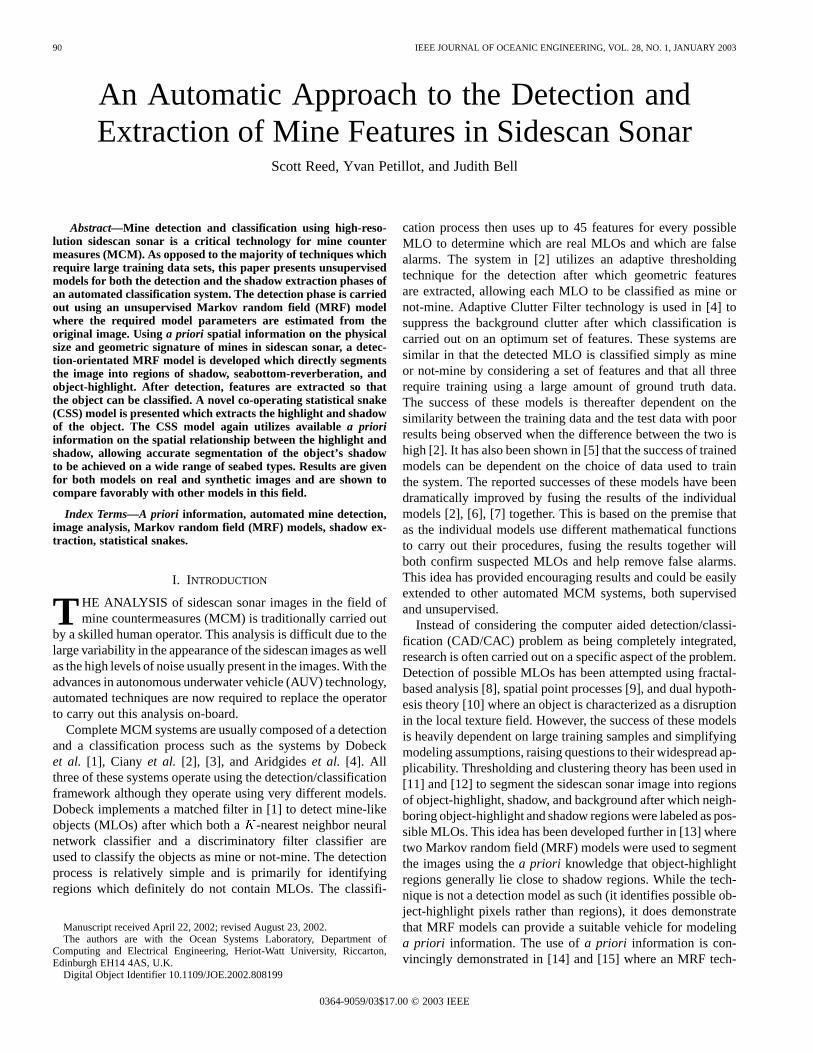
Fig. 3. Second-order neighborhood system with associated cliques and theirlabeling notations.

Fig. 4. Overview of the detection model.

The first term on the right-hand sideis the energy term relevant to the likelihood

function . The second term describes the depen-dency of label on the label values of the neighboring pixelsof where a second-order anisotropic model has been used.Fig. 3 shows the four allowed cliques for this neighborhood,thereby showing how or depending onthe relative position of the neighboring pixel to pixel.

The third term acts only on pixels with labelobject-highlight . This uses an adaptation of a potential

term derived in [13], utilizing thea priori information that amine highlight should have a shadow to the right of it (portconfiguration). The fourth term uses morea priori informationand favors the clustering of object pixels only ifthey are of the right size. This function models the belief thatmine-like signatures are in general compact and separated.

An overview of the entire detection-orientated segmentationprocess quantified in (2) can be seen in Fig. 4. The separatecomponents within this process will now be considered in detail.

C. Estimation of the Markovian Parameters and NoiseParameters

For the estimation of the Markovian parametersand the noise parameters, the

image is first considered to be composed of only two regions:shadow and nonshadow. The likelihood term for the shadowclass is assumed to be a Gaussian with meangray-level and variance and , respectively. The likeli-hood term for the seabottom-reverberation classis described by a shifted Rayleigh law with minimum gray-level

and variance , thereby requiring noise parametersto be estimated. Justification

for using a Rayleigh distribution for the seabottom-rever-beration class can be seen in [32]. This argues that isotropicseabed regions are described well by Rayleigh distributionswhile it is assumed that the luminance within shadow regionsis essentially due to electronic noise and so is described by aGaussian distribution.

As mine-like objects are knowna priori to be small and clus-tered [10], the estimation of these parameters without consid-eration to the third class object -highlight was ex-pected to yield accurate results. Determining estimates toand was done using the Iterative Conditional Estimation(ICE) model described in detail in [31], and [33] and summa-rized here. The ICE technique first requires initial estimatesand to the parameters and . The iterative techniquethen defines and to be the conditional expecta-tions of parameter estimators and , respectively, at itera-tion dependent on the data and the current param-eter fits and . Appealing to the law of large numbers,these terms are related by

(3)

(4)

Both and can therefore be calculated bydrawing realizations from the posterior distri-bution where , the number of realizations,is set to 1. The Gibbs Sampler was used to generate samplesfrom this posterior distribution which was represented by asimplified version of the posterior energy in (2). This gave theposterior energy term described by

(5)

The last two terms of (2) have been neglected as these dealwith the object -highlight class and are therefore notused in this parameter estimation step. For the ICE techniqueto work, initial estimates and to the model parametersare required, as is a method for determiningand at eachiteration.

1) Determining and : Determining the estimator ofthe Markov parameters, , is done by considering label field

and uses a least squares technique as developed by Derinetal. [34]. Defining as the second-order neighborhood of pixel

as shown in Fig. 3, the Markovian probability can be writtenas

(6)

where, using the labels in Fig. 3, we have

(7)

where and is the Kronecker delta function. Thisprobability describes the dependency of labelon the labelsof the pixels in neighborhood . For a given neighborhood ,the ratio of the probabilities of pixelbeing a shadow ( )


or a seabottom-reverberation ( ) pixel can be calculatedusing (6) and taking the logarithm to give

(8)

For each possible neighborhood configuration, the secondterm in (8) can be approximated using simple histogrammingwhere the number of times each configuration occurs in the labelfield is counted to give

(9)

This creates an over-determined set of equations for the fourunknowns which can be solved in a least-squares sense to pro-vide an estimate for the Markovian model parameters .

Determining the estimator of the noise parametersis achieved by considering the complete data and isobtained using a simple maximum-likelihood method wherethe individual components of can be determined by

(10)

(11)

(12)

(13)

where is the number of pixels with label.2) Obtaining Initial Estimates and : Once an

initial label field has been determined, the initialestimates and can be obtained using the techniquesdescribed in the previous section. is obtained byfirst splitting the image into nonoverlapping windows.Each window is assigned a vector, where .Each vector is composed of two components , the meangray level, and , the minimum gray level. These vectors arethen clustered into either a shadow or seabottom-reverberationgroup using a -means clustering algorithm [31]. From thisclustering algorithm, the maximum-likelihood estimates of

can be obtained. The label field can then beinitialized using simple maximum-likelihood considerations[essentially segmenting the image using only the first term onthe right-hand side of (5)]. From this, can be obtainedusing the least-squares method described in the previoussection. Starting from initial parameter estimates and ,the ICE model can thereafter produce more accurate estimates.

D. Obtaining and Updating Initial Object-Highlight NoiseParameters

The appearance of object-highlight regions in sidescan sonaris dependent on a large variety of factors such as the mate-rial and orientation of the object involved. It therefore cannotbe described by a well-defined noise law as with the shadowand seabottom-reverberation regions. However, due to the factthat the objects protrude above the seafloor and that they have

often have a higher degree of reflectivity than the seafloor, ob-ject-highlight regions are generally among the brightest partsof the sidescan image (which are typically quantized to 8 b).Teaching algorithms to model the object-highlight noise distri-bution based on training sets would prove problematic due tothe large number of variables that dictate the appearance of thehighlight regions. For instance, sonar images taken on the sameheading but different altitudes would produce very different re-sults. An AUV on a different heading altogether would likelyproduce an image unrecognizable as the same area of seabed.Due to these complexities, it is necessary to deduce the ob-ject-highlight noise distribution on a per-image basis, using adistribution that simply models the vaguea priori belief thatthe highlight regions are the brightest parts of the image. A nor-malized linear equation is used with the form

(14)

where is the Heaviside function, is the gradient of theline, is the intersect point, and are the minimumand maximum allowed gray levels and ensures the func-tion to be normalized within the allowed limits .Initially we have no information on the expected range of theobject-highlight pixels and so the conservative values of

, , , are allocated.is allocated the highest gray-level value in the image. This

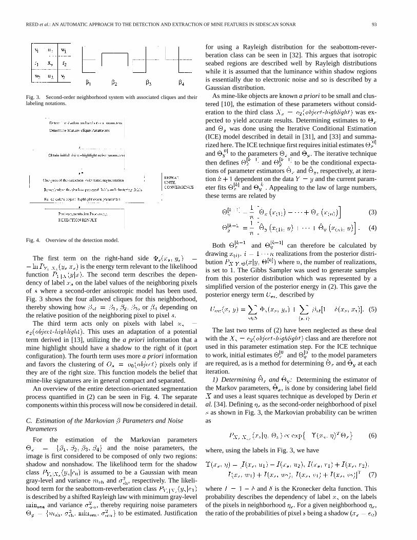
produces a normalized triangular function. Using these param-eter estimates for the object-highlight regions along with thefinal parameter estimates , the label field can be initial-ized for all three classes. This is demonstrated in Fig. 5 wherethree images containing mines are shown along with the initiallabeling for field prior to segmentation.

As Fig. 5 shows, the accurate parameter estimation ofusing the ICE technique has led to a good initialization for theshadow and seabottom-reverberation regions. The descriptionof the object-highlight regions is much poorer due to the lackof a priori information, highlighting the need for the two priorterms in (2) to provide an accurate segmentation.

As the detection-orientated segmentation continues, thepriors which affect the object-highlight pixels (thesetwo terms are explained in the next section) will begin toremove many of the false alarms allowing the noise distributionfor the object-highlight regions to be updated. This allowsthe numerical values used for initialization to be updated asthe segmentation proceeds. and are updated by aLeast-squares method similar to that used in the estimation of

where a general linear line is fitted to a histogram of thepixels labeled object -highlight .

Parameters and are estimated from the object-high-light histogram while , the normalizing constant, is calcu-lated by

(15)

E. Modeling the A Priori Information

Objects in sidescan sonar leave a recognizable signature char-acterized by a highlight region followed by a region of shadow.


Fig. 5. (a) Three images containing mines. (b) Initial three-class labeling of fieldX prior to the detection-orientated segmentation where black represents shadowregions, gray represents seabottom-reverberation regions and white represents object-highlight regions.

As discussed in Section II, the highlight regions of these ob-jects also generally appear in small dense clusters surroundedby regions of seabottom-reverberation or shadow. This knowna priori information can be modeled to increase the robustnessof the detection algorithm.

1) The Shadow Prior Energy Term:The termin (2) acts only upon pixels

with label object-highlight and discourages pixelsnot in the proximity of a shadow region from being labeled

object -highlight [13]. A priori information on thegeometry of the signature (all examples here are for portconfiguration) allow this criteria to become more specific inthat the shadow region must lie to the right of the highlightregion. We define a shadow pixel situated at row andcolumn of the image which generates a potential field

such that

(16)

where is the distance from pixel and controlsthe rate of drop-off of the potential field. This is set atthroughout to allow a smooth drop-off in the potential. Utilizingthe a priori information that the shadow is always to the rightof the highlight region in port configuration, we can express thetotal potential field at pixel as

(17)

where is the distance between pixels and , is theKronecker delta function, and is the Heaviside function.

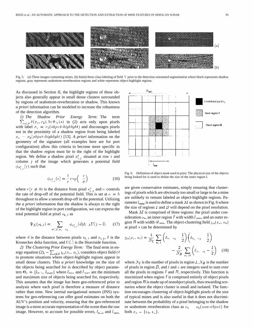
2) The Clustering Prior Energy Term:The final term in en-ergy equation (2), , considers object fieldto promote situations where object-highlight regions appear insmall dense clusters. Thisa priori knowledge on the size ofthe objects being searched for is described by object parame-ters where and are the minimumand maximum size of objects being searched for, respectively.This assumes that the image has been geo-referenced prior toanalysis where each pixel is therefore a measure of distancerather than time. New inertial navigational sensors (INS) sys-tems for geo-referencing can offer good estimates on both theAUV’s position and velocity, ensuring that the geo-referencedimage is a more accurate representation of the scene than the rawimage. However, to account for possible errors, and

Fig. 6. Definition of object mask used in prior. The physical size of the objectsbeing looked for is used to define the size of the inner region I.

are given conservative estimates, simply ensuring that cluster-ings of pixels which are obviously too small or large to be a mineare unlikely to remain labeled as object-highlight regions. Pa-rameter is used to define a mask as shown in Fig. 6 wherethe size of regions and will depend on the pixel resolution.

Mask is comprised of three regions: the pixel under con-sideration , an inner region with width , and an outer re-gion with width . The object-clustering fieldat pixel can be determined by

(18)

where is the number of pixels in region, is the numberof pixels in region , and and are integers used to sum overall the pixels in regions and , respectively. This function ismaximized when region is composed entirely of object pixelsand region is made up of nonobject pixels, thus rewarding sce-narios where the object cluster is small and isolated. The func-tion encourages clustering of object-highlight pixels of the sizeof typical mines and is also useful in that it does not discrimi-nate between the probability of a pixel belonging to the shadowor seabottom reverberation class as non-object forboth .


F. The Segmentation Process

Achieving the global minima of (2) is a computationallyhuge task. The iterated conditional modes (ICM) technique[28] dramatically lightens computational demands by swiftlyconverging onto a local minimum. Segmentation is carried outusing a raster scan where each pixel is considered in turn. Eachpixel is assigned a label so as to always minimize energy

in (2).After every sweep through the image, object fieldis up-

dated from label field . The shadow potential field isrecalculated for each pixeland the object-highlight noise pa-rameters are also recalculated. While these calculations shouldtheoretically occur after every pixel label change, real-time con-straints make this impractical and, in practice, good results areobtained with the updates being calculated after every sweep.

G. Postsegmentation Processing

The detection-orientated segmentation process producesa field which is segmented into regions of shadow,seabottom-reverberation, and object-highlight. While the lasttwo terms in (2) discourage regions of object-highlight whichdo not conform to the known mine signature in sidescan, falsealarms can occur. To remove these, a postsegmentation processis carried out. This process will first useto remove object-highlight regions which lie outside theacceptable size range. It will also remove object-highlightregions which do not lie in close proximity to a shadow regionby defining a maximum allowed distance . The set limitsfor these techniques need not be rigidly defined and could bemade case-specific. For example, if the model was lookingfor tethered mines, both the shadow potential and thepost-segmentation distance could be altered to detectthe expected signature left by such a mine. was set to 5pixels in this model.

1) The Size of the Object:Model parametersdescribe the minimum and maximum size of po-

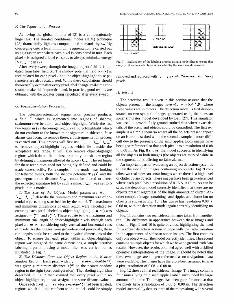
tential objects being searched for by the model. The maximumand minimum dimensions of each region were calculated byensuring each pixel labeled as object-highlight ( ) wasassigned— and . These equate to the maximum andminimum run length of object-highlight pixels through eachpixel , considering only vertical and horizontal runsof pixels. As the images were geo-referenced previously, theserun-lengths could be equated to the physical dimensions of theobject. To ensure that each pixel within an object-highlightregion was assigned the same dimensions, a simple iterativelabeling algorithm using a mode filter was carried out asillustrated in Fig. 7.

2) The Distance From the Object Region to the NearestShadow Region:Each pixel with object-highlightwas given a minimum distance to the nearest shadowregion to the right (port configuration). The labeling algorithmdescribed in Fig. 7 then ensured that every pixel within anobject-highlight region was assigned the same distance value.

Once each pixel object -highlight had been labeled,regions which did not conform to the model could be simply

Fig. 7. Explanation of the labeling process using a mode filter to ensure thatevery pixel within each object is described by the same size dimensions.

removed and replaced with seabottom-reverberationpixels.

H. Results

The detection results given in this section assume that theobjects present in the images have wherethese values are in meters. The detection model is first demon-strated on two synthetic images generated using the sidescansonar simulator model developed by Bell [27]. This simulatorwas used to provide fully ground truthed data where exact de-tails of the scene and objects could be controlled. The first ex-ample is a simple scenario where all the objects present appearon an isotropic seabed while the second example is more diffi-cult due to the presence of the sand ripples. Both images havebeen geo-referenced so that each pixel has a resolution of 0.08

0.08 m. As Fig. 8 shows, the model succeeds in identifyingall the objects in both images (the objects are marked white inthe segmentation), offering no false alarms.

An important part of evaluating an object detection system isto test the model on images containing no objects. Fig. 9 con-tains two real sidescan sonar images where there is a high levelof clutter but no objects. These images have been geo-referencedwhere each pixel has a resolution of 0.150.15 m. As can beseen, the detection model correctly identifies that there are noobjects present regardless of the high amounts of clutter. An-other complex image containing sand ripples and clutter but noobjects is shown in Fig. 10. This image has resolution 0.080.08 m, with the detection model again correctly identifying noobjects.

Fig. 11 contains two real sidescan images taken from anothertrial. The difference in appearance between these images andthose in Figs. 9 and 10 is quite obvious, highlighting the needfor a robust detection system to cope with the large variationin the appearance of sidescan sonar images. The first containsonly one object which the model correctly identifies. The secondcontains multiple objects for which we have no ground truth dataresults. However, the results obtained agree well with a skilledoperator’s interpretation of the image. It should be noted thatthese two images are not geo-referenced as no navigational datawere available. The images have therefore been assumed to havea pixel resolution of 0.08 0.08 m.

Fig. 12 shows a final real sidescan image. The image containsfour mines lying on a sand ripple seabed surrounded by largeamounts of clutter. The images has been georeferenced so thatthe pixels have a resolution of 0.08 0.08 m. The detectionmodel successfully detects three of the mines along with several


Fig. 8. (a) Synthetic image containing two mine-like objects and the detection-orientated segmentation result identifying all objects. (b) Synthetic image containingfour mine-like objects on a complex seabed and the detection-orientated segmentation result correctly identifying all objects.

Fig. 9. (a) Real sidescan image containing no mine-like objects and thedetection-orientated segmentation result which correctly detects no objects.(b) Another real sidescan image containing no mine-like objects and thedetection-orientated segmentation result correctly identifying no objects.

false alarms. The failure to detect the fourth mine arose from theregion behind the object having a relatively high gray level

Fig. 10. (a) Real Sidescan image containing no mines but high levels ofclutter and complex seabed types. (b) Detection-orientated segmentation modelcorrectly detecting no objects in the image.

therefore being labeled seabottom-reverberation. This causedthe post-segmentation phase to remove the fourth mine as it hadno accompanying shadow region. The false alarms detected allhave sizes and signatures comparable to a mine-like object andare a result of the image containing a lot of object-like clutter.With the final three-tier classification system, it is hoped thatthese detections will be removed after the classification phase(see Fig. 1). Using the classification stage to remove false alarmscould eventually allow the postsegmentation process of the de-tection model to be relaxed, thereby ensuring that the fourthmine in Fig. 12 is not removed.

I. Summary

This section has introduced an automated detection algo-rithm which conducts a detection-orientated segmentation ofthe image using an MRF model along witha priori spatialinformation on the expected signature of mines in sidescan.The model has been tested on real and synthetic images, both ofwhich contained clutter and a variety of seabed types. Results


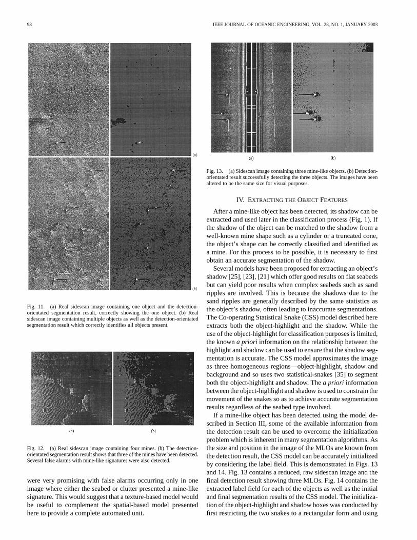
Fig. 11. (a) Real sidescan image containing one object and the detection-orientated segmentation result, correctly showing the one object. (b) Realsidescan image containing multiple objects as well as the detection-orientatedsegmentation result which correctly identifies all objects present.

Fig. 12. (a) Real sidescan image containing four mines. (b) The detection-orientated segmentation result shows that three of the mines have been detected.Several false alarms with mine-like signatures were also detected.

were very promising with false alarms occurring only in oneimage where either the seabed or clutter presented a mine-likesignature. This would suggest that a texture-based model wouldbe useful to complement the spatial-based model presentedhere to provide a complete automated unit.

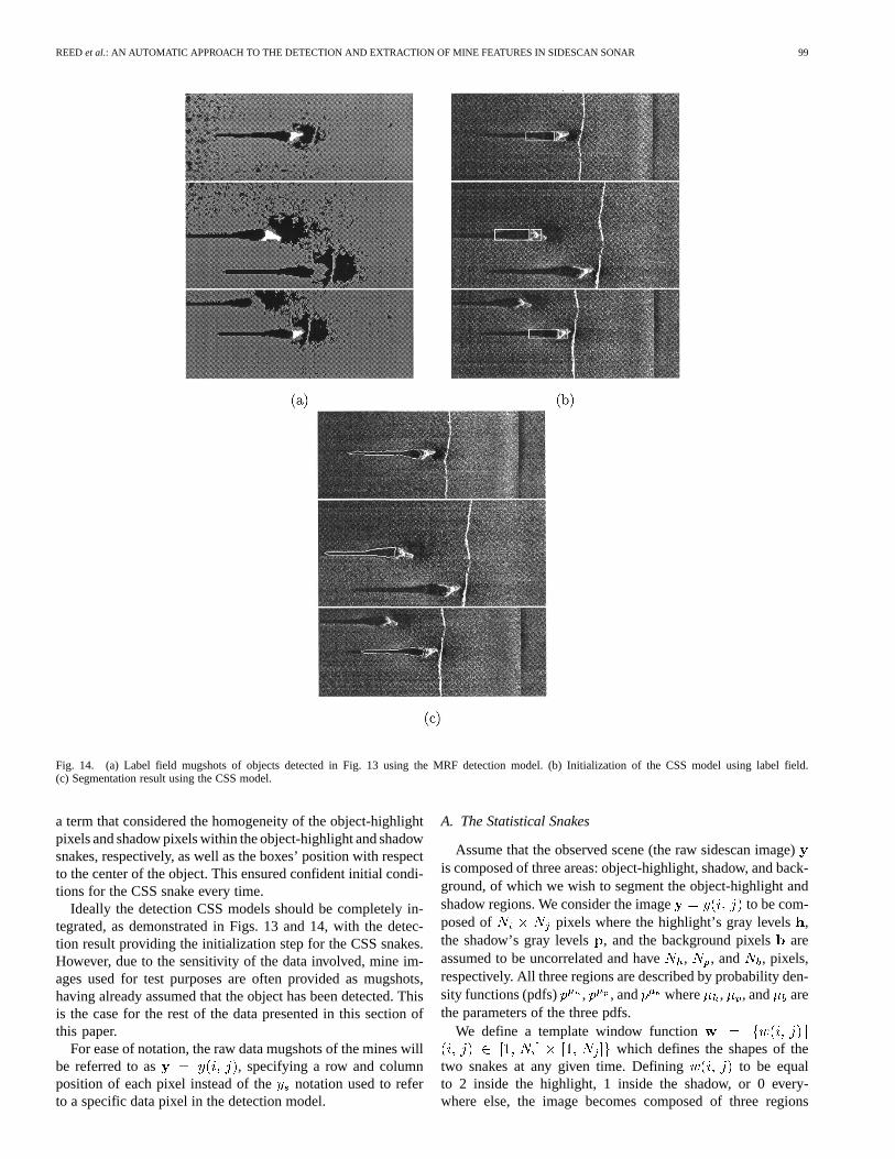
Fig. 13. (a) Sidescan image containing three mine-like objects. (b) Detection-orientated result successfully detecting the three objects. The images have beenaltered to be the same size for visual purposes.

IV. EXTRACTING THE OBJECTFEATURES

After a mine-like object has been detected, its shadow can beextracted and used later in the classification process (Fig. 1). Ifthe shadow of the object can be matched to the shadow from awell-known mine shape such as a cylinder or a truncated cone,the object’s shape can be correctly classified and identified asa mine. For this process to be possible, it is necessary to firstobtain an accurate segmentation of the shadow.

Several models have been proposed for extracting an object’sshadow [25], [23], [21] which offer good results on flat seabedsbut can yield poor results when complex seabeds such as sandripples are involved. This is because the shadows due to thesand ripples are generally described by the same statistics asthe object’s shadow, often leading to inaccurate segmentations.The Co-operating Statistical Snake (CSS) model described hereextracts both the object-highlight and the shadow. While theuse of the object-highlight for classification purposes is limited,the knowna priori information on the relationship between thehighlight and shadow can be used to ensure that the shadow seg-mentation is accurate. The CSS model approximates the imageas three homogeneous regions—object-highlight, shadow andbackground and so uses two statistical-snakes [35] to segmentboth the object-highlight and shadow. Thea priori informationbetween the object-highlight and shadow is used to constrain themovement of the snakes so as to achieve accurate segmentationresults regardless of the seabed type involved.

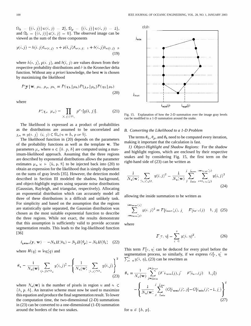
If a mine-like object has been detected using the model de-scribed in Section III, some of the available information fromthe detection result can be used to overcome the initializationproblem which is inherent in many segmentation algorithms. Asthe size and position in the image of the MLOs are known fromthe detection result, the CSS model can be accurately initializedby considering the label field. This is demonstrated in Figs. 13and 14. Fig. 13 contains a reduced, raw sidescan image and thefinal detection result showing three MLOs. Fig. 14 contains theextracted label field for each of the objects as well as the initialand final segmentation results of the CSS model. The initializa-tion of the object-highlight and shadow boxes was conducted byfirst restricting the two snakes to a rectangular form and using


Fig. 14. (a) Label field mugshots of objects detected in Fig. 13 using the MRF detection model. (b) Initialization of the CSS model using label field.(c) Segmentation result using the CSS model.

a term that considered the homogeneity of the object-highlightpixels and shadow pixels within the object-highlight and shadowsnakes, respectively, as well as the boxes’ position with respectto the center of the object. This ensured confident initial condi-tions for the CSS snake every time.

Ideally the detection CSS models should be completely in-tegrated, as demonstrated in Figs. 13 and 14, with the detec-tion result providing the initialization step for the CSS snakes.However, due to the sensitivity of the data involved, mine im-ages used for test purposes are often provided as mugshots,having already assumed that the object has been detected. Thisis the case for the rest of the data presented in this section ofthis paper.

For ease of notation, the raw data mugshots of the mines willbe referred to as , specifying a row and columnposition of each pixel instead of the notation used to referto a specific data pixel in the detection model.

A. The Statistical Snakes

Assume that the observed scene (the raw sidescan image)is composed of three areas: object-highlight, shadow, and back-ground, of which we wish to segment the object-highlight andshadow regions. We consider the image to be com-posed of pixels where the highlight’s gray levels,the shadow’s gray levels, and the background pixels areassumed to be uncorrelated and have, , and , pixels,respectively. All three regions are described by probability den-sity functions (pdfs) , , and where , , and arethe parameters of the three pdfs.

We define a template window functionwhich defines the shapes of the

two snakes at any given time. Defining to be equalto 2 inside the highlight, 1 inside the shadow, or 0 every-where else, the image becomes composed of three regions


, ,and . The observed image can beviewed as the sum of the three components

(19)

where , , and are values drawn from theirrespective probability distributions andis the Kronecker deltafunction. Without anya priori knowledge, the best is chosenby maximizing the likelihood

(20)

where

(21)

The likelihood is expressed as a product of probabilitiesas the distributions are assumed to be uncorrelated and

.The likelihood function in (20) depends on the parameters

of the probability functions as well as the template. Theparameters where are computed using a max-imum-likelihood approach. Assuming that the three regionsare described by exponential distributions allows the parameterestimates to be injected back into (20) toobtain an expression for the likelihood that is simply dependenton the sums of gray levels [35]. However, the detection modeldescribed in Section III modeled the shadow, background,and object-highlight regions using separate noise distributions(Gaussian, Rayleigh, and triangular, respectively). Allocatingan exponential distribution which can accurately model allthree of these distributions is a difficult and unlikely task.For simplicity and based on the assumption that the regionsare statistically quite separated, the Gaussian distribution waschosen as the most suitable exponential function to describethe three regions. While not exact, the results demonstratethat this assumption is sufficiently valid to provide accuratesegmentation results. This leads to the log-likelihood function[36]

(22)

where and

(23)

where is the number of pixels in region and. An iterative scheme must now be used to maximize

this equation and produce the final segmentation result. To lowerthe computation time, the two-dimensional (2-D) summationsin (23) can be converted to a one-dimensional (1-D) summationaround the borders of the two snakes.

Fig. 15. Explanation of how the 2-D summation over the image gray levelscan be modified to a 1-D summation around the snake.

B. Converting the Likelihood to a 1-D Problem

The terms , , and need to be computed every iteration,making it important that the calculation is fast.

1) Object-Highlight and Shadow Regions:For the shadowand highlight regions, which are enclosed by their respectivesnakes and by considering Fig. 15, the first term on theright-hand side of (23) can be written as

(24)

allowing the inside summation to be written as

(25)

where

(26)

This term can be deduced for every pixel before thesegmentation process, so similarly, if we express

, (23) can be rewritten as

(27)

for .


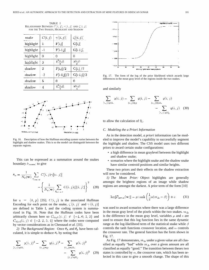
TABLE IRELATIONSHIP BETWEEN C(i; j), (i; j) AND �(i; j)

FOR THETWO SNAKES, HIGHLIGHT AND SHADOW

Fig. 16. Description of how the Huffman encoding system varies between thehighlight and shadow snakes. This is so the model can distinguish between theseparate regions.

This can be expressed as a summation around the snakesboundary to give

(28)

for [35]. is the associated HuffmanEncoding for each point on the snake, andare defined in Table I, and the coding system is summa-rized in Fig. 16. Note that the Huffman codes have beenarbitrarily chosen here so and

where the codes were computedby vector considerations as in Chesnaudet al. [35].

2) The Background Region:Once and have been cal-culated, it is simple to deduce by noting that

(29)

Fig. 17. The form of the log of the prior likelihood which awards largedifferences in the mean gray level of the regions inside the two snakes.

and similarly

(30)

to allow the calculation of .

C. Modeling the a Priori Information

As in the detection model,a priori information can be mod-eled to improve the model’s capability to successfully segmentthe highlight and shadow. The CSS model uses two differentpriors to award certain snake configurations:

• a high difference in mean graylevel between the highlightand shadow snake;

• scenarios where the highlight snake and the shadow snakehave similar centroid positions and similar heights.

These two priors and their effects on the shadow extractionwill now be considered.

1) The Mean Prior: Object highlights are generallyamongst the brightest regions of an image while shadowregions are amongst the darkest. A prior term of the form [10]

(31)

was used to award scenarios where there was a large differencein the mean gray level of the pixels within the two snakes.is the difference in the mean gray level, variablesand areused to ensure that this log function lies in the same dynamicrange as the log-likelihood term of the statistical snake whilecontrols the tanh functions crossover location, andcontrolsthe crossover rate. The general function has the form shown inFig. 17.

As Fig. 17 demonstrates, under a given value are all clas-sified as equally “bad” while over a given amount are allclassified as equally “good.” The transition between theses twostates is controlled by, the crossover rate, which has been se-lected in this case to give a smooth change. The shape of this


Fig. 18. A priori knowledge on the relationship between an objects highlightand its shadow can be used to constrain the two snakes.

prior term stops the two snakes from simply collapsing to en-sure a high .

2) The Position Prior: The presence of sand ripples canoften lead to an incorrect shadow extraction due to the rippleshadows corrupting the results. However, in the cases wherean object highlight is present, it is possible to become moreassertive as to which shadow regions are due to the object andwhich are not. We first define the variables, , , and

as described in Fig. 18 where is the coordinate of thecenter of snake and is the maximum height ofsnake such that

(32)

where is the boundary of snake, is the number of pixelson the boundary edge, and where

. We can now define the differences and where

(33)

(34)

The ideal scenario is when both and are equal tozero and so we define the allowed spread in these variables asa Gaussian distribution with mean 0. Assuming that the distri-butions of and the are independent of each other, thecombined log prior term can be written as a sum of the indi-vidual log terms to give

(35)

where and and are constants. These determine the penaltyfor moving away from the ideal case where both andequal zero. is a constant to ensure that the prior lies in thesame dynamic range as .

3) Determining the Prior Constants:Both the mean and theposition priors discussed previously contain constants whichneed to be determined before the segmentation can begin. Thisis carried out as a presegmentation calculation. The two snakesare initially restricted to only four points each and kept in rect-angular form. A quick iterative process is carried out wherethe rectangular snakes’ positions and dimensions (height, width,position, and distance apart) are altered randomly within an al-lowed range. At each position, the log-likelihood of the statis-tical snake is measured using (22). To simplify this process, bothboxes have the same and height while the lengths of thehighlight and shadow boxes are kept atand , respectively.This restricts the size of the parameter space to four parameters( , , , and ) where is the coordinate of the centerof the highlight box and is the distance between the two boxes.This simplistic box model for the two snakes allows a thorough

Fig. 19. (a) Two images containing mines with initial CSS snakes shown.(b) Segmentation result obtained using the SS model. (c) Segmentation resultobtained using the MRF/CS model. (d) Segmentation result obtained using theCSS model.

search through the parameter space for estimating the dynamicrange of the likelihood model as well as finding a favorable ini-tial starting point for the two snakes.

As with all deformable models, a good initial starting point ishighly desirable. If the mugshot image of the object came fromthe detection model detailed in Section III, an accurate initial-ization of the CSS model is possible using the label field, asshown in Figs. 13 and 14, where accurate size and positionaldata can be extracted. However, for the data shown in this sec-tion for which noa priori size or positional information is avail-able, the initialization of the two snakes is carried out while theprior constants are being estimated and is determined by usingthe snake positions which maximize the difference in the meangray levels of the two box-snakes .

Using the rectangular snakes, the log likelihoodfrom (22) was calculated iteratively. and wereallocated the lowest and highest log likelihood found, re-spectively. Defining the largest difference in log likelihood

allowed the prior constants to be definedas

(36)

(37)

These values ensured that prior terms had roughly the samedynamic range as the log likelihood . This is importantfor ensuring that the relative importance of the different termscan be controlled so that the log-likelihood term canremain the dominant segmentation term while the prior termssimply constrain the snakes’ movements in a sensible manner.

D. The Segmentation Process

The segmentation process has to maximize the posteriorfunction

(38)


Fig. 20. (a) Three images containing mines with initial CSS snakes shown. (b) Segmentation result obtained using the SS model. (c) Segmentation result obtainedusing the MRF/CS model. (d) Segmentation result obtained using the CSS model.

where is a smoothing prior [35] andare weights used to control the impor-

tance of each term.A multiscale maximum approach was used to segment the

highlight and shadow regions where both snakes were initializedwith only four points. The iterative approach randomly selects apoint after which its displacement from its old position is againdetermined randomly. The displacement uses two 1-D Gaussianproposal distributions such that, for the-displacement,

where is drawn from a Gaussian with mean andstandard deviation . After each displacement, a checkmust be carried out to ensure that none of the snake segmentscross (the model operates under the assumption that the snakesare simply connected) after which the decision on whether tokeep or reject the new configuration is made.

New points were added when convergence had been achievedwith the present set of snake points (this was defined to bereached when the best fit solution had not changed for 200 it-erations). new points were added between pointsandwhere was the integer solution to , simplybeing the distance between the two points. This allows the snakeprogressively more flexibility as the algorithm proceeded. Ac-curate segmentation results were seen to be obtained after twoadditions of points.

Although all three terms lie within the same dynamic range,it was important that the statistical snake term remainedthe dominant term. and were maintained at 0.2 throughoutwhile was initialized at 0.0 and incremented by 0.05 everytime new points were added. This ensured that the snakes main-tained a smooth form as they were given more flexibility ofmovement.

E. Results

Results are given on seven real and two synthetic sidescanimages to allow the model to be tested over a large range ofconditions. The performance of the CSS model is compared to

the performance of two alternative models. The first is a singlestatistical snake (SS) model as described in [23]. The secondis a classical-based snake technique as discussed in [24] wherethe image is first binarized using a two-class hierarchical MRFmodel (MRF-CS). The snake is driven by an energy term whichconsiders both the homogeneity of shadow pixels inside thesnake and the proximity of the snake to the edges of the bi-narized image described by an edge potential field [25]. As anaside, it should be noted that the MRF-CS model generally pro-vides a smoother contour than the SS model due to its edge po-tential term. Rather than insisting that the MRF-CS snake liedirectly on the shadow boundary, the edge potential term allowsthe snake to simply lie in the proximity of the edge and so gen-erally acts as a smoothing agent to the model.

The initial starting point for the CSS model’s snakes are alsoshown. As discussed before, when using raw sidescan data, theresults from the detection model outlined in Section III can beused to accurately initialize the CSS model. However, as mostof the data was obtained as mugshots, the CSS model was ini-tialized using the method described in Section IV-C3 while theprior constants were being estimated. While this gave a poorerinitialization point than using the detection result, the model isstill successful in obtaining the correct segmentation. The othertwo models only segment the shadow and so were initializedusing the CSS model’s shadow initialization position.

Fig. 19 contains two images of objects lying on a flat seabed.The first image contains an object with clear object-highlightand shadow regions ensuring both the SS and the CSS modelsprovided an accurate segmentation result. The MRF-CS solu-tion detects a smaller shadow region as the MRF two-class seg-mentation removed part of the shadow region. The second imagecontains a sharp drop in graylevel with range as well as an ob-ject with very little highlight. Both the SS and the CSS modelprovide good segmentations (even though there is no distinc-tive highlight region) while the MRF-CS model gives a poorsegmentation. This was due to the extreme range variation ingraylevel leading to a poor MRF two-class segmentation.


Fig. 21. (a) Four images containing mines on a sand ripple seabed with initial CSS snakes shown. (b) Segmentation result obtained using the SS model.(c) Segmentation result obtained using the MRF/CS model. (d) Segmentation result obtained using the CSS model.

Fig. 20 contains three noisy images of objects (one cylinderand two spheres) lying on a flat seabed. All three objects haveeither an indistinctive or no highlight region. However, theshadow regions are relatively clear and all three models provideaccurate shadow segmentation results.

Fig. 21 contains two real and two synthetic images where theobjects can be seen lying on sand ripple seabeds. In all fourcases, both the SS and the MRF-CS models provide poor seg-mentation results as they cannot distinguish between the objectshadow and the ripple shadows. The CSS model, constrained byits priors, achieves good segmentation results in all four cases.

F. Summary

A novel CSS model has been presented for extractingthe shadow of unknown objects in Sidescan imagery forfuture classification. Whilst the extraction of the shadow isrelatively simple on a flat seabed, the presence of clutter orripple shadows confuses the situation leading to inaccuratesegmentations using standard techniques.A priori informationon the expected signature of objects in Sidescan imagerywas used to constrain the snakes’ movement so that accuratesegmentation results could be obtained regardless of the seabedtype involved. The CSS model’s extraction of the highlightregion is also useful in the later classification phase, where thesize and orientation information of the highlight region can beused to constrain the possible object shapes which could haveproduced the observed shadow region.

V. OVERALL CONCLUSION AND FUTURE RESEARCH

This paper has presented automated models for both objectdetection and feature extraction in sidescan imagery. The detec-tion model used spatiala priori knowledge on the size and ge-ometry of object signatures in sidescan within the framework of

an MRF model to provide accurate detection results even whenlarge amounts of clutter were present. The model provides aninteresting alternative to the current trend of trained detectionmodels as in [1], [9], [2], and [14], making it applicable for awide range of data without the problem of requiring suitabletraining data. This model was tested on both real and syntheticdata offering good results in all cases.

Once an object has been detected, its shadow can beextracted for future classification. A novel CSS model waspresented which extracted both the object highlight and itsshadow. This technique demonstrated how the inclusion ofapriori information could again provide more accurate results.Specifically, the problems inherent when considering complexseabed backgrounds as noted in [17] and [24] did not impactthe accuracy of the results obtained using the CSS model. TheCSS model was favorably compared with a statistical snakemodel and a MRF-based model with results presented on realand synthetic data.

Although this paper has concentrated on the detection ofMLOs in sidescan imagery, suitable alteration of the priorsinvolved would allow the described techniques to be applied toother fields such as pipeline or trawling scar detection. Futureresearch will concentrate on using the CSS model results forclassification purposes as well as developing a texture-orien-tated detection model thereby producing the building blocksfor a complete automated classification system.

ACKNOWLEDGMENT

The authors would like to thank B. Zerr at GESMA for pro-viding many of the sidescan images for both the detection andthe CSS models. They would also like to thank QinetiQ for pro-viding data as well as the SACLANT Center, La Spezia, Italy,for allowing the inclusion of data from the BP’02 test runs.


REFERENCES

[1] G. J. Dobeck, J. C. Hyland, and L. Smedley, “Automated detection/clas-sification of sea mines in sonar imagery,”Proc. SPIE—Int. Soc. Optics,vol. 3079, pp. 90–110, 1997.

[2] C. M. Ciany and W. Zurawski, “Performance of Computer Aided De-tection/Computer Aided Classification and data fusion algorithms forautomated detection and classification of underwater mines,” inProc.CAD/CAC Conf., Halifax, NS, Canada, Nov. 2001.

[3] C. M. Ciany and J. Huang, “Computer aided detection/computer aidedclassification and data fusion algorithms for automated detection andclassification of underwater mine,” inProc. MTS/IEEE Oceans Conf.and Exhibition, vol. 1, 2000, pp. 277–284.

[4] T. Aridgides, M. Frenandez, and G. Dobeck, “Adaptive 3-dimensionalrange–crossrange-frequency filter processing string for sea mine classi-fication in side-scan sonar imagery,”Proc. SPIE, vol. 3079, pp. 111–122,1997.

[5] R. Balasubramanian and M. Stevenson, “Pattern recognition for under-water mine detection,” inProc. CAD/CAC Conf., Halifax, NS, Canada,Nov. 2001.

[6] T. Aridgides, M. Ferdandez, and G. Dobeck, “Fusion of adaptive algo-rithms for the classification of sea mines using high resolution side scansonar in very shallow water,” inProc. MTS/IEEE Oceans Conf. and Ex-hibition, vol. 1, 2001, pp. 135–142.

[7] G. J. Dobeck, “Algorithm fusion for automated sea mine detection andclassification,” inProc. MTS/IEEE Oceans Conf. and Exhibition, vol. 1,2001, pp. 130–134.

[8] L. M. Linett, S. J. Clarke, C. St. J. Reid, and A. D. Tress, “Monitoring ofthe seabed using sidescan sonar and fractal processing,” inProc. Conf.Underwater Acoustics Group, 1993, vol. 15, pp. 49–64.

[9] L. M. Linett, D. R. Carmichael, S. J. Clarke, and A. D. Tress, “Textureanalysis of sidescan sonar data,” inProc. IEE Conf. Texture Analysis inRadar and Sonar London, U.K., Nov. 1993.

[10] B. R. Calder, L. M. Linnet, and D. R. Carmichael, “Spatial stochasticmodels for seabed object detection,”Proc. SPIE—Int. Soc. Opt. Eng.,vol. 3079, pp. 172–182, 1997.

[11] S. G. Johnson and M. A. Deaett, “The application of automated recogni-tion techniques to side-scan sonar imagery,”IEEE J. Oceanic Eng., vol.19, pp. 138–144, Jan. 1994.

[12] S. Guillaudeux, “Some image tools for sonar image processing,” inProc.CAD/CAC Conf., Halifax, NS, Canada, Nov. 2001.

[13] M. Mignotte, C. Collet, P. Perez, and P. Bouthemy, “Three class Mar-kovian segmentation of high resolution sonar images,”Comput. Vis.Image Und., vol. 76, pp. 191–204, Dec. 1999.

[14] B. Calder, “Bayesian spatial models for SONAR image interpretation,”Ph.D. dissertation, Heriot-Watt University, September 1997.

[15] B. R. Calder, L. M. Linnet, and D. R. Carmichael, “Bayesian approach toobject detection in sidescan sonar,”IEE Proc.—Vis. Image Signal Proc.,vol. 45, no. 3, 1998.

[16] M. F. Doherty, J. G. Landowski, P. F. Maynard, G. T. Uber, D. W. Fries,and F. H. Maltz, “Side scan sonar object classification algorithms,” inProc. 6th Int. Symp. Unmanned Untethered Submersible Technology,1989, pp. 417–424.

[17] J. A. Fawcett, “Image-based classification of side-scan sonar detec-tions,” in Proc. CAD/CAC Conf., Halifax, NS, Canada, Nov. 2001.

[18] P. H. Pidsley and M. A. Way, “Processing for CAD and image basedCAC,” in Proc. CAD/CAC Conf., Halifax, NS, Canada, Nov. 2001.

[19] C. Xu and J. L. Prince, “Snakes, shapes and gradient vector flow,”IEEETrans. Image Processing, vol. 7, pp. 359–269, Mar. 1998.

[20] M. Kass, A. Witkin, and D. Terzopoulos, “Snakes: Active contourmodels,”Int. J. Comput. Vis., pp. 321–331, 1987.

[21] V. J. Myers, “Image segmentation using iteration and fuzzy logic,” inProc. CAD/CAC Conf., Halifax, NS, Canada, Nov. 2001.

[22] I. Quidu, Ph. Malkasse, G. Burel, and P. Vilbe, “Mine classification usinga hybrid set of descriptors,” inProc. OCEANS MTS/IEEE Conf. andExhibition, vol. 1, 2000, pp. 291–297.

[23] S. Reed, J. Bell, and Y. Petillot, “Unsupervised segmentation of objectshadow and highlight using statistical snakes,” inProc. GOATS Conf.,La Spezia, Italy, 2001.

[24] S. Reed, Y. Petillot, and J. Bell, “Unsupervised mine detection and anal-ysis in side-scan sonar: A comparison of Markov Random Fields andstatistical snakes,” inProc. CAD/CAC Conf., Halifax, NS, Canada, Nov.2001.

[25] M. Mignotte, C. Collet, P. Perez, and P. Bouthemy, “Hybrid genetic op-timization and statistical model-based approach for the classification ofshadow shapes in sonar imagery,”IEEE Trans. Pattern Anal. MachineIntell., vol. 22, pp. 129–141, Feb. 2000.

[26] I. Quidu, Ph. Malkasse, G. Burel, and P. Vilbe, “Mine classificationbased on raw sonar data: An approach combining Fourier descriptors,statistical models and genetic algorithms,” inProc. OCEANS MTS/IEEEConf. and Exhibition, vol. 1, 2000, pp. 285–290.

[27] J. Bell, “A model for the simulation of sidescan sonar,” Ph.D. disserta-tion, Heriot-Watt University, August 1995.

[28] J. Besag, “On the statistical analysis of dirty pictures,”J. Roy. Statist.Soc., vol. B-48, no. 3, pp. 259–302, 1986.

[29] M. L. Comer and E. J. Delp, “Segmentation of textured images usinga multiresolution Gaussian autoregressive model,”IEEE Trans. ImageProcessing, vol. 8, pp. 408–420, Mar. 1999.

[30] S. Geman and D. Geman, “Stochastic relaxation, Gibbs distributions,and Bayesian restoration of images,”IEEE Trans. Pattern Anal. MachineIntell., vol. PAMI-6, pp. 721–741, Nov. 1984.

[31] M. Mignotte, C. Collet, P. Perez, and P. Bouthemy, “Sonar image seg-mentation using an unsupervised hierarchical MRF model,”IEEE Trans.Image Processing, vol. 9, pp. 1216–1231, July 2000.

[32] K. W. Stewart, D. Chu, S. Malik, S. Lerner, and H. Singh, “Quantitativeseafloor characterization using a bathymetric sidescan sonar,”IEEE J.Oceanic Eng., vol. 19, pp. 599–610, Oct. 1994.

[33] W. Pieczynski, “Statistical image segmentation,”Mach. Graphics Vis.,vol. 1, no. 1/2, pp. 261–268, 1992.

[34] H. Derin and H. Elliott, “Modeling and segmentation of noisy and tex-tured images using Gibbs Random Fields,”IEEE Trans. Pattern Anal.Machine Intell., vol. PAMI-9, pp. 39–55, Jan. 1987.

[35] C. Chesnaud, P. Refregier, and V. Boulet, “Statistical region snake-basedsegmentation adapted to different physical noise models,”IEEE Trans.Pattern Anal. Machine Intell., vol. 21, pp. 1145–1157, Nov. 1999.

[36] C. Chesnaud, V. Page, and P. Refregier, “Improvement in robustness ofthe statistically independant region snake-based segmentation methodof target-shape tracking,”Opt. Lett., vol. 23, pp. 488–491, Apr. 1998.

Scott Reed received the M.Phys. degree in astro-physics (with Honors) from Edinburgh University,Edinburgh, U.K., in 1999 and the M.Sc. degree ininformation technology from Heriot-Watt Univer-sity, Edinburgh. He is currently working toward thePh.D. degree at Heriot-Watt University where heis researching object detection and classificationmodels in underwater image processing.

His current research interests include Bayesianstatistics, Markov random field models, patternrecognition techniques, image segmentation, and

fuzzy logic.

Yvan Petillot received the Ph.D. degree from theUniversite de Bretagne Occidentale in 1996. Hisdissertation work focused on real-time patternrecognition using optical processors.

He is currently a Lecturer in the school ofEngineering and Physical Sciences in Heriot-WattUniversity, Edinburgh, U.K. Since finishing hisdoctoral work, he has been working on varioussuccessful research projects in the field of imageprocessing (ESPRIT III, HICOPOS, MAST III andARAMIS) and is currently an investigator on two

European Union projects (FPV AMASON and AUTOTRACKER). His fieldsof interests include image analysis and understanding, sonar image processing,navigation, and sensor fusion.

Judith Bell received the M.Eng. degree (with Merit)in electrical and electronic engineering and the Ph.D.degree from Heriot-Watt University, Edinburgh,U.K., in 1992, and 1995, respectively. Her thesisexamined the simulation of sidescan sonar images.

She is currently a Lecturer at Heriot-Watt Univer-sity and is extending the modeling work to examinemodeling of high-frequency active sonars and the useof such models for the verification and developmentof algorithms for processing sonar images.

An automatic approach to the detection and extraction of...

Documents

Transcript of An automatic approach to the detection and extraction of...