AN AUTOMATED METHOD OF PREDICTING CLEAR-AIR TURBULENCE

THESIS

Brian L. Belson, Captain, USAF

AFIT/GM/ENP/04-02

DEPARTMENT OF THE AIR FORCE AIR UNIVERSITY

AIR FORCE INSTITUTE OF TECHNOLOGY

Wright-Patterson Air Force Base, Ohio

APPROVED FOR PUBLIC RELEASE; DISTRIBUTION UNLIMITED

The views expressed in this thesis are those of the author and do not reflect the official policy or position of the United States Air Force, Department of Defense, or the United States Government

AFIT/GM/ENP/04-02

AN AUTOMATED METHOD OF PREDICTING CLEAR-AIR TURBULENCE

THESIS

Presented to the Faculty

Department of Engineering Physics

Graduate School of Engineering and Management

Air Force Institute of Technology

Air University

Air Education and Training Command

In Partial Fulfillment of the Requirements for the

Degree of Master of Science in Meteorology

Brian L. Belson, BS

Captain, USAF

March 2004

APPROVED FOR PUBLIC RELEASE; DISTRIBUTION UNLIMITED.

AFIT/GM/ENP/04-02

AN AUTOMATED METHOD OF PREDICTING CLEAR-AIR TURBULENCE

Brian L. Belson, BS Captain, USAF

Approved:

iv

AFIT/GM/ENP/04-02

Abstract

Clear-air turbulence (CAT) prediction is vitally important to military aviation and

the successful completion of Department of Defense (DoD) operations such as air to air

refueling and new national defensive weapon systems such as directed energy platforms.

The unique mission requirements of military aircraft often require strict avoidance of

turbulent regions. Traditionally, weather forecasters have found it difficult to accurately

predict CAT. In order to forecast regions where CAT might occur, forecasters must first

determine the location of breaking waves caused by either Kelvin-Helmholtz instabilities

or topographically forced internal gravity waves (mountain waves) in the atmosphere.

The United States Air Force (USAF) 15th Operational Weather Squadron (15th OWS)

requested an updated method of predicting CAT and this request was ranked as one of the

highest priority research needs by the HQ USAF Director of Weather, Deputy Chief of

Staff for Air and Space Operations.

A new method of forecasting turbulence was developed in this work and the

operational model was delivered to the 15th OWS for immediate inclusion into their

operations. This method combines output from the Knapp-Ellrod index and the Naval

Research Laboratory’s Mountain Wave Forecast Model (MWFM) onto a single chart.

Displaying these tools together allows forecasters to view both causes of CAT

simultaneously. Furthermore, a new visualization tool is developed that allows a

forecaster to view several layers at the same time as well as a composite chart to greatly

reduce the time required to produce turbulence charts by OWS forecasting centers

v

worldwide. Tests of forecast accuracy, as determined by pilot reports (PIREPS), between

charts currently produced by USAF OWSs and this new method were compared, with the

new method producing far superior forecast results. This method revolutionizes the way

USAF OWSs produce turbulence charts to help the Air Force satisfy each of its core

competencies; especially information superiority, rapid global mobility, and precision

engagement.

vi

Acknowledgements

I would like to thank those people who most helped me complete this research.

First and foremost, I thank my thesis advisor Lt Col Michael Walters for his guidance and

advice throughout my research. He was the master at subtly steering me towards

solutions to the problems I encountered. Also, I would like to thank the other members

of my committee, Lt Col Ron Lowther and Maj Robin Benton, for the guidance in their

respective areas of expertise.

In addition, I appreciate the help in implementing the Ellrod-2 index from David

Knapp and Gordon Brooks at AFWA. I owe a special thanks to Earl Barker for taking

his personal time to provide me with the bulk of the model data I used, without which the

research would not have gone so smoothly. I also owe thanks to Dr. Steve Eckermann at

NRL for his assistance with the MWFM.

Lastly, I wanted to thank my family for their help in editing this paper. To my

classmates, thanks for the laughs and pretending to being interested in my thesis topic

when you had your own to worry about. Thanks Capt Scott Miller, for your assistance in

figuring out the MWFM. And finally, to my wife, thank you for the support and always

asking, “Why aren’t you done yet?”

Brian L. Belson

vii

Table of Contents

Page

Abstract .............................................................................................................................. iv Acknowledgements............................................................................................................ vi List of Figures .................................................................................................................... ix List of Tables ...................................................................................................................... x I. Introduction .................................................................................................................... 1

1.1 Statement of Problem................................................................................................ 2 1.2 Research Objectives.................................................................................................. 3 1.3 Research Approach ................................................................................................... 3

II. Literature Review.......................................................................................................... 6

2.1 Kelvin-Helmholtz Instability .................................................................................... 6

2.1.1 Knapp-Ellrod Index ......................................................................................... 12 2.2 Mountain Waves ..................................................................................................... 14

2.2.1 Mountain Wave Forecast Model V1.1............................................................. 18 2.2.2 Mountain Wave Forecast Model V2.1............................................................. 19

2.3 Pilot Reports............................................................................................................ 21 III. Methodology............................................................................................................... 24

3.1 Overview................................................................................................................. 24 3.2 Data ......................................................................................................................... 25

3.2.1 Model Input Data ............................................................................................. 25 3.2.2 MWFM Input Data .......................................................................................... 26 3.2.3 Ellrod 2 Input Data........................................................................................... 27 3.2.4 PIREP Input Data............................................................................................. 27

3.3 Index Configuration................................................................................................ 28 3.3.1 MWFM Configuration ..................................................................................... 28 3.3.2 Ellrod 2 Index Configuration ........................................................................... 31

3.4 Implementation ....................................................................................................... 32 3.4.1 Index Implementation ...................................................................................... 32 3.4.2 PIREP Index Assignment Implementation ...................................................... 34 3.4.3 Composite Index Implementation.................................................................... 35 3.4.4 GrADS Implementation ................................................................................... 35 3.4.5 Turbulence Layer Viewer Implementation ...................................................... 37

3.6 Statistical Methods.................................................................................................. 42

viii

3.6.1 Threshold Determination ................................................................................. 42 3.6.2 PIREP Verification .......................................................................................... 44

IV. Results......................................................................................................................... 46

4.1 Introduction............................................................................................................. 46 4.2 Threshold Determination ........................................................................................ 46 4.3 Forecast Comparison .............................................................................................. 49

V. Conclusions and Recommendations ............................................................................ 54

5.1 Conclusions............................................................................................................. 54 5.2 Recommendations................................................................................................... 56

5.2.1 Recommendations to AFWA........................................................................... 56 5.2.2 Future Research Recommendations................................................................. 57

Appendix A: Detailed Computations................................................................................ 60 Appendix B: CONUS what2do Script .............................................................................. 62 Appendix C: GrADS Scripts............................................................................................. 71 Appendix D: Turbulence Viewer Code ............................................................................ 77 Appendix E: FORTRAN Code Used in Computing Indices ............................................ 83 Bibliography ..................................................................................................................... 94 Glossary ............................................................................................................................ 98 Vita.................................................................................................................................. 100

ix

List of Figures

Figure Page

1. Contingency table used to verify turbulence forecasts .................................................. 9

2. A classic model of a mountain wave ........................................................................... 15

3. Example of output from MWFM V2.1 ........................................................................ 30

4. Example of accuracy of MWFM display using GrADS.............................................. 33

5. Example composite chart............................................................................................. 36

5: Example composite chart............................................................................................. 37

6. Turbulence layer viewer .............................................................................................. 38

7. Examples of composite level output ............................................................................ 50

x

List of Tables

Table Page

1. Statistics used in index studies..................................................................................... 10

2. Comparison of indices for data collected..................................................................... 11

3. Turbulence intensity threshold for Ellrod index .......................................................... 13

4. List of turbulence intensity values ............................................................................... 28

5. List of flight levels based on pressure.......................................................................... 39

6. Thresholds determined for indices............................................................................... 47

7. Statistics for different regions...................................................................................... 49

8. Test method contingency table .................................................................................... 51

9. OWS forecast contingency table.................................................................................. 51

10. Verification statistics ................................................................................................. 52

1

AN AUTOMATED METHOD OF PREDICTING CLEAR-AIR TURBULENCE

I. Introduction

Over the history of aviation, atmospheric turbulence has had a huge impact on

flight cost and safety. For example, turbulence cost United States commercial and

military aircraft over $25 million annually from 1963 to 1965 (Hopkins 1977). More

recently, turbulence related incidents accounted for over half of all the commercial carrier

accident and incident reports between the years 1990 and 2000, according to the National

Transportation Safety Board (Sharman et al. 2000). Generally, there are two categories

of atmospheric turbulence of concern to aviators: turbulence associated with convective

clouds and turbulence that occurs outside of convective clouds. Pilots and weather

forecasters are primarily concerned with turbulence occurring outside of convective

clouds, or clear-air turbulence (CAT), as it rarely offers any visual indications.

CAT is defined as any turbulence in the free atmosphere of interest to aerospace

operations that is not in or adjacent to visible convective activity, including turbulence

found in cirrus clouds not in or adjacent to visible convective activity (Hopkins 1977).

There are two widely accepted causes of CAT; either standing waves in the lee of a

mountain barrier (mountain waves) or vertical wind shear in a stably stratified layer

(Kelvin-Helmholtz instabilities) (Hopkins 1977). Current methods of prediction have a

difficult time accurately forecasting CAT. This forecast challenge exists in part because

forecasters must use synoptic scale analysis techniques and coarse resolution numerical

models to predict a mesoscale phenomenon (Ellrod 1989).

2

1.1 Statement of Problem

Whether supporting commercial or military aircraft, forecasters spend significant

time and effort predicting CAT. For example, USAF weather personnel make turbulence

charts for 12, 18, 24, 30, 36, and 48 hour forecasts once per day to support United States

Army and Air Force aviation. These charts should include regions of light, moderate,

severe, and extreme turbulence time phased for three hours before and after the forecast

hour between 10,000 and 50,000 feet mean sea level (MSL) (Air Force Manual 15-129

2001). However, in practice, most weather squadrons only forecast for moderate or

greater (MOG) turbulence. The range between 10,000 and 50,000 feet is also represented

as FL100-FL500. Past experience has shown these charts take significant time to

prepare.

USAF weather forecasters use numerous methods, some of which are subjective,

to predict CAT (15 OWS 2003). Subjective methods, such as conceptual models and

rules of thumb, rely heavily on individual forecaster skill and experience, both of which

vary greatly between USAF weather forecasters. Since USAF weather centers predict

turbulence for large, geographically diverse portions of the earth, subjective methods are

largely responsible for the substantial length of time required in building these charts.

Further increasing the time required to build turbulence charts, different methods

of CAT prediction capture one cause of turbulence or the other, but not both. This

limitation forces forecasters to use multiple tools while building their products. The

method developed here provides a tool that displays indices representing both causes of

3

CAT on the same graphic, allowing the forecaster to quickly determine regions where

either might occur.

1.2 Research Objectives

The primary goal of this research is to provide Air Force weather squadrons with

an invaluable tool for timely and accurate prediction of CAT. Specifically, the objectives

of this research are to provide USAF weather personnel with:

1. A method to quickly determine likely regions of turbulence caused by either

Kelvin-Helmholtz instabilities or mountain waves;

2. An objective tool requiring little human interpretation that provides superior

forecasts to those currently requiring significant human interpretation;

3. A web-based visualization tool that provides a three-dimensional, layer-by-layer

view of the atmosphere; and,

4. An initial determination of the potential benefit of using the Mountain Wave

Forecast Model (MWFM) to predict turbulence in the troposphere.

1.3 Research Approach

The Ellrod-2 index, as described by Ellrod and Knapp (1991), was chosen to

depict Kelvin-Helmholtz instabilities. It computes a value based on vertical wind shear,

horizontal deformation, and convergence. This index is built within the Operational

Production System Version 2 (OPS II) software used by most OWSs. Further

4

substantiating its use, this index compared favorably with other indices in a study by

Brown et al. (2000).

The MWFM version 1 and 2 were chosen to predict mountain waves in this study.

These models were developed at the Naval Research Laboratory (NRL) to predict regions

of stratospheric turbulence caused by breaking mountain waves. The MWFM is

computed from atmospheric modeled data and a global ridge database. Application of

the model to two case studies of tropospheric turbulence suggested it might apply there as

well (Eckermann et al. 2000). In this study, both versions of the model were tested to

determine if both indices added value to a forecast.

The indices were calculated over the continental United States (CONUS) using

the National Center for Environmental Prediction’s (NCEP) Global Forecast System

(GFS) model, formerly known as the Aviation model (AVN). The MWFM retrieved the

data using file transfer protocol (FTP) and stored the data locally for access by a program

that computes the Ellrod-2 index. To facilitate timely completion of this research, only

the analysis, 12-hour forecast, and 24-hour forecast were produced.

Initially, the output from the indices were compared with pilot reports (PIREPS),

as provided by the Air Force Combat Climatology Center (AFCCC), to determine the

threshold for each index. After determining the thresholds, the indices were combined

into a single graphic for each 50 mb layer of the atmosphere that contained FL100-FL500

and integrated into a multiple layer viewer for forecasting. Additionally, a chart was

made containing a composite view of all layers. Finally, 14 days of forecasts using these

charts were developed. The accuracy of these forecasts and forecasts produced by the

15th Operational Weather Squadron (OWS) were verified against PIREPS data.

5

The remainder of this thesis provides details on the indices chosen and the

methods used to forecast turbulence. Chapter two provides background information on

the causes of CAT and the chosen indices. Then, chapter three describes the

implementation of the forecast method. Chapter four discusses the results of the

threshold determination and the forecast comparison. Finally, chapter five provides

conclusions and suggests future research regarding this topic.

II. Literature Review

2.1 Kelvin-Helmholtz Instability

Meteorologists have long recognized and accepted breaking waves caused by

Kelvin Helmholtz instabilities as a primary cause of clear-air turbulence. Kelvin-

Helmholtz instabilities occur in regions of strong vertical wind shear (VWS) in stably

stratified air (Hopkins 1977). Vertical wind shear is simply the change in wind speed

with height while stable stratification requires more explanation.

Stably stratified air suggests relatively small vertical density differences. A

modified form of the ideal gas law relates pressure, temperature, and density to each

other by:

P RTρ= (1)

where P is the pressure, ρ is density, R is the dry air gas constant 287.04 1 1J Kg K− −⋅ ⋅ ,

and T is the temperature. Typically, atmospheric pressure and temperature decrease with

height. Equation 1 suggests that changing pressure or temperature while holding the

other constant changes the density. The equation suggests decreasing pressure causes

density to decrease while decreasing temperature causes density to increase. Because the

effects from decreasing pressure outweigh the effects from decreasing temperature

(pressure decreases more rapidly with height), the overall effect is that density decreases

with height. However, the more rapidly the temperature decreases for a given pressure

decrease, the more gradual the decrease in density. Essentially, the more rapidly the

temperature decreases with height the greater the stable stratification of the air.

7

To simplify the mathematics involved in determining the stability, potential

temperature is used. Potential temperature is defined as the temperature a parcel of air

would have if it were compressed or expanded adiabatically from its existing pressure

and temperature to a reference pressure level (Wallace and Hobbs 1977). Basing

calculations on potential temperature instead of standard temperature simplifies the

determination of the stratification of the atmosphere.

Mathematically, the Richardson number (Ri) relates the two necessary conditions

for Kelvin-Helmholtz instabilities as a ratio:

2

gzRi

Vz

θθ

∂∂=

∂ ∂

v (2)

where g is the acceleration due to gravity, θ is the potential temperature, zθ∂

∂ is the

change in potential temperature with height (representing the stability of the layer), and

Vz

∂∂

v

is the vertical wind shear. In order for turbulence to occur, the Richardson number

must be less than a critical value of 0.25 (Thorpe 1969), which requires some

combination of low static stability and high vertical wind shear. It is hypothesized that a

minimum value of wind shear is required for these instabilities to form regardless of the

value of the Richardson number. This implies that meeting the 0.25 threshold is a

necessary, not a sufficient, condition for CAT not associated with mountain waves

(Ellrod and Knapp 1991).

8

It is also important to note that Kelvin-Helmholtz instabilities are possible for

small wavelengths, regardless of the wind shear and static stability (Ray 1986).

However, small wavelengths do not cause sufficient turbulence to influence aircraft.

According to Sharman et al. (2000), these waves need to be on the scale of 100 m long to

affect large airframes.

Often these waves occur in air with insufficient moisture for clouds to form.

When this happens they do not have any visible billow clouds associated with them. If

sufficient moisture is present these waves look similar to breaking ocean waves. Like an

ocean wave, the larger the amplitude of the wave prior to it breaking, the more intense the

resulting turbulence.

Forecasters have relied on synoptic pattern recognition and, more recently,

numerical model indices to predict these instabilities, with limited success. Both of these

approaches attempt to use large scale features to determine regions that are likely to

contain these relatively small scale events (Ellrod 1989). Based on the 100 m wavelength

requirement, numerical model grid points would need to be spaced 10 m apart to

accurately predict these waves (Sharman et al. 2000). Further limiting the effectiveness

of these indices is the poor temporal resolution of both synoptic and model data. Kelvin-

Helmholtz waves are short-lived (often less than 30 minutes) while synoptic and model

data are typically valid every six or twelve hours.

With the introduction of computer models, researchers have recognized the

usefulness of indicators other than the Richardson number to predict CAT associated with

Kelvin-Helmholtz instabilities. Although a Richardson number less than 0.25 is

9

theoretically a good indicator of turbulent conditions, it is not well-suited to computer

models for several reasons:

1. It is difficult to accurately calculate the index using a numerical model due

to coarse vertical resolution (Ellrod and Knapp 1991).

2. Computations using data from rawinsondes, the best source of

measurement, often lead to Richardson values between 0.25 and 1.0 in

turbulent regions (Ellrod and Knapp 1991).

3. Values of Richardson less than 0.25 occur in both turbulent and smooth

areas (Ellrod and Knapp 1991).

4. A detailed statistical study produced poor correlation between the

Richardson number and CAT (Dutton 1980).

Yes NoForecasted

Yes

No C D

Observed

A B

Figure 1. Contingency table used to verify turbulence forecasts

Recently, Brown et al. (2000) conducted a comparative study of 11 CAT

algorithms. The 11 algorithms tested were Brown-1 (Brown 1973), Colson-Panofsky

(Colson and Panofsky 1965), DTF3, DTF4, DTF5 (Marroquin 1985, 1998), Empirical

10

Dutton (Dutton 1980), Ellrod-1, Ellrod-2 (Ellrod and Knapp 1991), Endlich (Endlich

1964), ITFA (Sharman et al. 2000), and the Richardson number (Drazin and Reid 1981;

Kronebach 1964). In Brown et al. (2000), contingency tables such as the one depicted in

Figure 1 were produced for each index. In Figure 1, observed values are based on

PIREPS while forecasted values are based on an index.

Table 1. Statistics used in index studies Statistic Definition Description PODy A/(A+C) Probability of Detection of yes observations.

Probability of yes observations that were correctly forecasted.

PODn D/(B+D) Probability of detection of no observations. Probability of no observations that were correctly forecasted.

FAR B/(A+B) False Alarm Rate. Probability of yes forecasts that were incorrect.

CSI A/(A+B+C) Critical success index. Number of correct yes forecasts relative to number of yes forecasts or observations.

PC (A+D)/(A+B+C+D) Proportion correct. The proportion of yes or no forecasts that were forecasted properly.

Bias (A+B)/(A+C) Bias. Frequency of yes forecasts relative to yes observations.

HSS 2(AD-BC)/ [(A+C)(C+D)+(A+B)(B+D)

Heidke Skill Score. PC normalized by the number of forecasts expected to be correct.

GSS (A-C2)/[(A-C2)+B+C) where C2=(A+B)(A+C)/

(A+B+C+D)

Gilbert Skill Score. CSI corrected for the value of YY that would be expected by chance.

TSS PODy+PODn-1 True Skill Score. Measure of discrimination. Using PIREPS and automated vertical accelerometer (AVAR) observations of “g”

forces, as reported by United Airlines flights, as observed values and index thresholds as

forecasted values, contingency tables were produced for each index in the study. The

contingency tables were used to compute the statistics described in Table 1. For reasons

discussed in detail in Section 2.3, several statistics such as false alarm rate (FAR), bias,

11

and critical skill index (CSI) can be somewhat misleading. When considering these

statistics, the probability of detection, yes and no (PODy and PODn) and the true skill

score (TSS) are fairly reliable indicators of an index’s forecast ability.

Table 2. Comparison of indices for data collected

Algorithm ThresholdPODy

(All)PODy

(MOG)PODn

(PIREPs)PODn

(AVARs) TSSAIRMETs -- 0.57 0.64 0.70 0.66 0.34Brown-1 9x10-5 0.58 0.62 0.63 0.58 0.25

Colson-Panofsky -1000 0.58 0.63 0.61 0.53 0.24DTF3 0.7 0.63 0.68 0.63 0.63 0.31DTF4 2.5 0.63 0.67 0.57 0.60 0.24DTF5 0.15 0.56 0.59 0.66 0.68 0.25

Empirical Dutton 25 0.62 0.66 0.57 0.57 0.23Ellrod-1 4x10-7 0.61 0.66 0.66 0.64 0.32Ellrod-2 4x10-7 0.61 0.66 0.63 0.59 0.29Endlich 0.225 0.63 0.66 0.53 0.55 0.19

ITFA 0.13 0.57 0.62 0.67 0.65 0.29Richardson # 4 0.58 0.63 0.66 0.64 0.29

Essentially, the reports were broken into two categories: one concerned with any

turbulence and another with turbulence of moderate or greater (MOG) intensity. The

results are listed in Table 2. The data used in Table 2 was adapted from Brown et al.

(2000) and was collected between 21 December 1988 and 31 March 1999 for flights

above 20,000 ft. Table 2 shows that DTF3, Ellrod-1 and -2 and ITFA performed the best

overall. However, it is apparent the difference between PODy values for most of the

indices used in this study was relatively small. This result may be attributable to the

strong similarity in the terms involved in the underlying equations for the various indices.

Additionally, this table highlights the measurable improvement in skill every index

experiences when predicting MOG turbulence.

12

2.1.1. Knapp-Ellrod Index. To predict turbulence caused by Kelvin-Helmholtz

instabilities, Knapp and Ellrod developed two indices known as Ellrod-1 and Ellrod-2

(Ellrod and Knapp 1991). These indices are almost identical; however, because the

convergence term tends to be an order of magnitude smaller than the other terms, Ellrod-

1 scales it out. The indices are found by computing the product of the sum of

deformation and convergence at a pressure level with vertical shear (Ellrod and Knapp

1991). The indices are derived from a version of Petterson’s (1956) equation for

frontogenic intensity:

0.5 ( (cos 2 ) )TTA DEF CVGn

β∂ = + ∂ (3)

2 2DEF DST DSH= + (4)

u vDSTx y

∂ ∂= −∂ ∂

(5)

v uDSHx y

∂ ∂= +∂ ∂

(6)

u vCVGx y

∂ ∂= − + ∂ ∂ (7)

where TA is the time rate of change of the temperature gradient on a constant pressure

surface, Tn

∂∂

is the magnitude of the temperature gradient normal to the isotherms, DEF is

the square root of the sum of the squares of the stretching (DST) and shear (DSH)

deformation, β is the angle between the isotherms and the axis of dilatation (stretching

axis in deformation flow), and CVG is convergence. The temperature gradient term is

related to vertical wind shear by the thermal wind equation:

13

dT fT Vdn g z

∂=∂

ur

(8)

where f is the coriolis parameter, T is the temperature, g is the gravitational acceleration

and Vz

∂ ∂

uv

is the vertical wind shear. After retaining the significant terms, equation (3)

simplifies to:

1 ( )TI VWS DEF= (9)

2 ( )TI VWS DEF CVG= + (10)

To determine the thresholds for the indices, Ellrod and Knapp (1991) compared

forecasted events of turbulence to PIREPS. Table 3 lists the resulting thresholds. Air

Force Global Weather Central (AFGWC), now known as the Air Force Weather Agency

(AFWA), calculated 2TI , or Ellrod-2, from the AFGWC global spectral model (GSM)

and High-Resolution Analysis System (HIRAS). The National Meteorological Center

(NMC) calculated 1TI , or Ellrod-1, from the National Meteorological Center Nested Grid

Model and Aviation Model to determine their values.

Table 3. Turbulence intensity threshold for Ellrod index Turbulence Intensity AFGWC NMC NGM NMC AVN

LGT-MDT 4MDT 8 4 2

MDT-SVR 12 8 4

The contingency table (see Figure 1) verification statistics at both AFGWC and

NMC showed some statistical skill for several criteria. For this study, the probability of

detection (POD) is the PC as outlined in Table 1. The POD was above 70% for both

14

AFGWC and NMC. The FAR (as described in Table 1) was 22% for the aviation model

(AVN), 36% for the nested grid model (NGM) and 30-48% for AFGWC.

It is important to remember the mesoscale, short-lived nature of CAT and the

relatively poor pilot report sampling of CAT identified regions when considering the high

probability of false alarms. These indices predict regions where conditions are favorable

for CAT to develop and not where it is actually occurring. The problem with PIREP

sampling is discussed further in Section 2.3.

Additionally, in a comparative study from November 1989 to April 1990, the

Ellrod Index compared well with the Empirical Dutton Index, both having similar POD

and FAR (Ellrod and Knapp 1991). The Dutton index was determined using linear

regression software from the University of California Los Angeles (Dutton 1980).

Dutton compared PIREP data to several potential indicators of CAT including the rate of

change of Richardson number (following the flow), horizontal wind shear, vertical wind

shear, wind speed, vertical velocity, horizontal gradient of vertical velocity, vorticity, and

deformation. Using the regression software, it determined an equation using the sum of

the square of vertical wind shear and horizontal wind shear as the best predictor of

turbulence.

2.2 Mountain Waves

Mountain waves have long been recognized as a cause for CAT. They typically

form when the normal component of the wind to the mountain is 10 m/s or more. They

are known to propagate 200km downstream of the mountain that causes them and their

15

intensity is usually maximized 1300m above and below the tropopause (Hopkins 1977).

Figure 2 shows a classic model of a mountain wave and areas of turbulence produced by

it (Chandler 1987).

Figure 2. A classic model of a mountain wave

Mountain waves are a type of internal gravity wave. An internal gravity wave is

caused by the combined force of gravity and buoyancy on a parcel of air displaced

vertically (NRL 2003). When displaced, the forces of gravity and buoyancy are typically

no longer in balance. This imbalance causes the parcel to accelerate vertically until it

reaches a level where the forces are again in balance. In an unstable environment, an

upward displaced air parcel is warmer than its surroundings. This parcel will continue to

accelerate upward away from the original layer. In a stable environment, an upward

16

displaced air parcel is cooler than its surroundings. In this case the force of gravity is

greater than buoyancy and the parcel accelerates downward toward (and beyond) its

original level. This acceleration past its original level leaves it warmer than its

surroundings and now the buoyancy force overcomes gravity. This causes the parcel to

accelerate upward towards its original level. The situation repeats itself causing the

parcel to oscillate vertically and laterally about some point in the horizontal plane (NRL

2003). In the case of mountain waves, this motion is continually forced by a mountain

range.

The frequency with which the air parcel oscillates vertically is known as the

Brunt-Väisälä frequency and is expressed mathematically as:

2 gNzθ

θ∂=∂

(11)

where N is the Brunt-Väisälä frequency and θ is the potential temperature. The

magnitude of the Brunt-Väisälä frequency is based on the static stability of the

environment. N2 also makes up the numerator in computing the Richardson number for

Kelvin-Helmholtz instabilities.

Based on the discussion in Holton (1992), the dispersion relation relates the

frequency of oscillation to the wave number. This relationship determines whether the

phase speed is a function of wavenumber and whether the wave pattern changes shape

(disperses). In the case of topographically forced gravity waves which are stationary with

respect to the ground, the dispersion relation is:

2

2 22

Nm ku

= − (12)

17

where m is the vertical wavenumber, u is the mean wind flow perpendicular to the

mountain range, and k is the horizontal wavenumber.

In equation 12, it is possible for m2 to be less than zero. In this case, the waves

are vertically trapped. Typically, flow over narrow ridges produces vertically trapped

waves. Narrow ridges tend to cause smaller wavelengths and thus larger values of

horizontal wavenumber. Additionally, small stability or a large perpendicular component

of the wind might cause vertically trapped waves. In either case, vertically trapped waves

typically decay exponentially with height.

When m2 is greater than or equal to zero, the waves are vertically propagating.

Vertically propagating waves occur with some combination of small mean perpendicular

flow, large stability, and large horizontal wavelength. Vertically propagating waves must

transport energy upward because the ground prevents downward propagation. Vertically

trapped waves also propagate energy upward but the energy decays with height. Also, it

is possible for both wave types to exist simultaneously (Neiman and Shaw 2003). In any

case, wave energy propagates upward away from the ground, although vertically trapped

wave amplitude decreases.

In the vertically propagating case, the amplitude of the wave grows with height as

the air becomes less dense (NRL 2003). Occasionally, the wave breaks and turbulence

results. The severity of the turbulence depends on the amplitude of the wave when it

breaks. The amplitude growth with height explains why mountain wave turbulence tends

to become more severe at higher altitudes.

Until recently, forecasters have relied on rules of thumb and rawinsonde

observation (RAOB) data to predict the occurrence of mountain waves. When using

18

RAOB data, they assessed the likelihood of turbulence based on software such as the

HiCAT (High Altitude CAT) analysis module which looks for “S” shaped temperature

patterns in three adjacent, distinct layers and computes the parameter based on the lapse

rate, mixing layer, depth of the “S” layer and the “S” layer vertical temperature difference

(Sinclair and Kuhn 1991). Recently, numerical model algorithms such as the Mountain

Wave Forecast Model (MWFM) have been developed and show potential for predicting

mountain wave turbulence in the troposphere (Eckerman et al. 2000).

2.2.1 Mountain Wave Forecast Model V1.1. Dr. Bacmeister (1993) of the Naval

Research Laboratory introduced MWFM V1.1. MWFM V1.1 calculates the distribution

of mountain waves forced by air flow over a set of ridges contained in a ridge database.

The ridge database was generated using a global topography dataset, compiled by the

National Center for Atmospheric Research (NCAR). This dataset was used to determine

ridge latitude, longitude, height, width, and orientation. MWFM V1.1 combines this

information and a two-dimensional hydrostatic gravity wave model to determine the

severity and extent of the waves generated by each ridge. For a detailed description of

the algorithm used in determining the ridge database, refer to Bacmeister et al. (1993).

According to Bacmeister et al. (1994), MWFM V1.1 derives a turbulence estimate

using the following method. First, the following assumptions are made: wave crests

generated by a ridge remain parallel to the ridge, the waves generated by the flow over

the ridge are hydrostatic, and the average momentum flux of the waves remains constant

with height until the wave breaks. The first calculation uses the perpendicular component

of the wind to each ridge to determine the stratification frequency profile over that ridge.

19

Next, the first guess wave displacement at each level is calculated using the following

equation:

;*

;

( ) ( ) ( )( ) ( )

( ) ( ) ( )k k

k kk k

z N z U zz z z

z z N z z U z zρ

δ δρ

⊥

⊥

+ ∆ =+ ∆ + ∆ + ∆

(13)

which is basically a ratio of the product of density ρ , stratification frequency kN , and

perpendicular component of the wind ;kU ⊥ at two adjacent levels. If this value exceeds

the saturation limit, it is reduced to equal the saturation limit. To compute the wave

displacement at the surface, the minimum of the saturation limit at the surface and a

multiple of the ridge height parameter is determined. The ridge height parameter is based

on the deviation of the ridge height from the surrounding topography. That value is

multiplied by a factor of four for the comparison.

Whenever the wave amplitude approaches or exceeds the saturation limit, some of

the energy is assumed to contribute to convective and shear instability. This results in

turbulence. Turbulence intensity is the difference between momentum flux computed for

two adjacent levels. Momentum flux is proportional to the terms in equation 13. Due to

the relatively simple, inexpensive calculations required, MWFM V1.1 is able to produce

timely, world-wide forecasts for altitudes up to the mesosphere (Eckerman et al. 2000).

For a more detailed look at the equations involved in calculating MWFM V1.1, refer to

Appendix A.

2.2.2. Mountain Wave Forecast Model V2.1. MWFM V2.1 addressed some of the

simplifications made by V1.1, at the expense of computation time, in an effort to more

accurately model mountain wave dynamics. The primary changes included the

20

conversion from two to three dimensions and from hydrostatic to non-hydrostatic

calculations. Although, the model was primarily designed for stratospheric turbulence, it

has shown promise for use in the middle and upper portions of the troposphere

(Eckerman et al. 2000).

According to Marks and Eckermann (1995), MWFM V2.1 is calculated using a

ray tracing model. The ray tracing model tracks the trajectory and amplitude deviations

of individual waves propagating through the atmosphere. In MWFM V2.1, a user-

defined number of rays are launched from each ridge with a pattern that depends on the

ratio of ridge width to length (Eckermann et al. 2001). In the case of a wide ridge, the

rays are launched at equidistant angles from 0-180° on the downwind side of the ridge.

The closer a ray is to the 90° angle, the higher the initial magnitude it is given. In the

case of an isolated peak, the rays take on a pattern similar to one created by a ship’s wake

and the rays are assigned similar initial amplitudes. Typically, 18 rays are launched from

each ridge with the MWFM V2.1.

Each ray is assigned initial values of longitude, latitude, and altitude.

Additionally, the horizontal wavenumber, ground-based frequency and other terms are

chosen such that the vertical group velocity is positive (Marks and Eckermann 1995).

This ensures the wave energy is propagated upward. Next, the wave amplitude is

determined by calculating the vertical flux of wave action. This flux is determined by

multiplying the vertical group velocity and the wave action density together. The wave

action density is simply the wave energy density divided by the intrinsic (Lagrangian)

frequency of the wave. The vertical flux of wave action is then integrated to find the

change in the vertical flux of wave action, which is used to find the wave amplitude

21

(Allen 2003). Once the wave amplitude is known, the calculations discussed in section

2.2.1 are applied to determine the turbulence intensity. For a detailed description of

MWFM V2.1, refer to Marks and Eckermann (1995).

According to Eckermann as cited in Allen (2003), the MWFM V2.1 also accounts

for the effects of friction and blocking using an arbitrary scaling factor and the local

Froude number respectively. An arbitrary scaling factor accounts for friction by reducing

the wind speed in the calculations. The local Froude number is the ratio of kinetic energy

to potential energy. When the Froude number is on the order of one, the effective height

of the terrain and the wave amplitude are reduced to account for blocking effects.

2.3 Pilot Reports

PIREPS are commonly considered the best method available for verifying

turbulence forecasts. These reports are typically reported by the aircrew over the radio,

but some aircraft have equipment which automatically records weather information.

Aircrews typically base the intensity of the turbulence they report on their subjective

interpretation while automated reports typically determine turbulence intensity by

measuring the center of gravity acceleration peaks. Different sources have related

different values of these peaks to different turbulence intensity. Current World

Meteorological Organization (WMO) standards use the following thresholds: light (0.15

g ≤ g* <0.5 g), moderate (0.5 g ≤ g* ≤ 1.0g), and severe (g* > 1.0 g) to quantify CAT

(WMO-No. 958 2003). These values are based on g* being the acceleration deviations

22

from the standard 1.0 g acceleration. The system reports turbulence measurements from

these sensors as turbulence type while aircrews report turbulence intensity.

PIREPS of turbulence (or lack of turbulence) are typically entered into a 2X2

contingency table with forecasts of turbulence (or lack of turbulence) as in Figure 1. The

values in these tables are then used with equations such as those listed in Table 1 to

summarize the skill of a forecast method (Brown and Young 2000).

Despite being the best verification tool available, using PIREPS does pose several

important problems. First, these reports frequently rely on a pilot’s subjective

interpretation of the severity of the turbulence encountered instead of relying on an

objective, quantitative value. This may lead to inconsistencies in the reporting of CAT

severity. Second, aircraft do not systematically and completely sample a grid to

definitively determine the presence of CAT (Brown and Young 2000). Essentially, an

aircraft usually flies a fairly direct route between two points instead of flying a grid

pattern over a region. A simulation study conducted by Brown and Young (2000)

demonstrates the inaccuracy in computing quantities such as FAR, bias, and other

statistics when using PIREPS for CAT verification. In that study, various percentages

of “yes”, “no”, or “yes” and “no” PIREPS were removed from a sample of 10,000

PIREPS and the various indices were recomputed. As larger percentages of PIREPS

were removed, the PODy and PODn values remained relatively constant. However, the

FAR, bias, and CSI changed significantly when a portion of either the “yes” or “no”

PIREPS were removed (not both). Removal of “yes” PIREPS resulted in increased FAR,

bias, and CSI while removal of “no” PIREPS resulted in decreased FAR, bias, and CSI.

This suggests a strong dependence on the relative frequency of “yes” or “no” PIREPS to

23

the FAR (resulting from PIREP sample having different probability distribution function

than the actual turbulence) and that high FAR is less significant than it might initially

seem.

There are several potential problems with accelerometer data although they are

more objective than PIREPS. First, depending on the size, altitude, and airspeed of the

aircraft or the nature of the turbulence, the accelerometer may read different values on the

accelerometer for the same turbulence encounter. Furthermore, the pilot may take actions

that modify the attitude of the aircraft and cause the accelerometer value to change.

These two effects limit the application of AVAR data as a tool in determining turbulence

intensity.

24

III. Methodology

3.1 Overview

The primary goal of this research was to provide the weather forecaster with a

quick, accurate method of developing turbulence charts that incorporate both primary

causes of CAT. To best achieve that goal, the needs for accuracy and speed were

addressed separately. This provided one distinct advantage. The speed with which the

turbulence charts get developed is independent of the quality of the underlying indices.

Clearly, the forecaster aids must be as skillful as possible to produce the most accurate

charts. Over time, the quality and resolution of the model might improve or a superior

new index might be developed. Regardless, the actual method of developing the charts

does not have to change, making implementation of improvements seamless to the

forecaster building the charts.

To capture turbulence caused by Kelvin-Helmholtz instabilities, the Ellrod-2

index was chosen. This index was chosen for two reasons. First, past research has

identified the Ellrod-2 index as being relatively skillful in predicting turbulence (Brown

et al. 2000). Second, the Ellrod-2 index is built into the software currently used by USAF

weather squadrons. This allows for easy integration of this method into OWS operations.

The Mountain Wave Forecast Model was chosen to identify turbulence caused by

mountain waves. As discussed previously, there are two versions of the model and for

this study both versions were tested. The MWFM was chosen for two reasons also.

Primarily, this model has shown some potential in predicting turbulence in the

25

troposphere caused by mountain waves (Eckermann et al. 2000). Additionally, the

MWFM is already being implemented at AFWA to predict stratospheric turbulence. The

modifications required to implement the model at tropospheric levels should be relatively

easy.

The Ellrod-2 index and MWFM indices were calculated in a window from 20N-

60N and 140W-30W. All but 29 of the analyses from May 20, 2003 to October 15, 2003

were used, along with PIREPS, to determine the thresholds. Additionally, the 12-hour

and 24-hour forecast data were used to make forecasts from October 21, 2003 to October

27, 2003 and from November 5, 2003 to November 12, 2003. These forecasts were

verified against PIREPS. Finally, 12-hour and 24-hour operational forecasts produced by

USAF weather squadrons from October 21, 2003 to October 27, 2003 and from

November 5, 2003 to November 12, 2003 were also verified with PIREPS.

3.2 Data

3.2.1 Model Input Data. The GFS model data were downloaded from the NCEP FTP

site. The GFS model is run four times daily although this research only used the 00Z and

12Z model runs. The model also forecasts out to 120 hours. This research only looked at

the analysis, 12-hour forecast, and 24-hour forecast. Horizontally, the GFS model uses

spectral basis functions with resolution T254. This amounts to approximately 0.5° x 0.5°

grid point spacing in the horizontal. Vertically, the GFS model is composed of 64 sigma

layers with emphasis below 800 mb and above 100 mb. This research used the layers

between 800 mb and 100 mb. The data files used in this study consisted of 1°x1° global,

26

gridded model data in the gridded binary (GRIB) format. More detail on the GFS model

is available at the NCEP web site (NCEP 2003). The FTP was performed by either the

MWFM software or by other methods that stored the data locally. The MWFM was

called from a script which first determined if the data were available locally before

attempting to retrieve the data from NCEP using FTP.

The retrieved data were stored on a 36 gigabyte hard drive. To reduce the storage

space required by these large data files, the data was compressed by GNU zip software

available for download on-line. Compression reduced the file sizes to about 80% of their

original size. This resulted in a saving of about 5 megabytes (MB) on an approximately

26 MB file retrieved from AFWA. The data stored in a local archive was retrieved from

the same FTP site but the files were trimmed to include only 0-90N latitude and 180W-0

longitude instead of the entire earth. Compression on these files resulted in a savings of

about 1 MB on a 5.5 MB file. Using the 5.5 MB data files required modification of the

MWFM and Ellrod-2 index code to account for the different starting and ending latitude

and longitude associated with those files. Finally, a third set of data files only included

the necessary model fields for the necessary levels on the global grid. These files were

reduced from about 10 MB to about 8 MB using compression software.

3.2.2 MWFM Input Data. The MWFM contains a variable that determines the source of

the model data. Based on data availability, the “ftpoption” variable was used with either

a “0” option or a “2” option. The “0” option causes the model to retrieve its data locally

and not to erase the data after the model run is complete. The “2” option causes the

model to retrieve the data from the NCEP FTP site and not to erase the data after the

27

model run is complete. The MWFM used four fields from the GFS model. These

include the absolute temperature, geopotential height, U wind component, and V wind

component. These fields were used by the MWFM equations to calculate turbulence for

every 50 millibar (mb) layer between 100 mb and 750 mb with the highest layer being the

100-150 mb layer and the lowest being the 700-750 mb layer. These layers encompass

the entire section of the atmosphere necessary to produce turbulence charts from FL100

to FL500.

3.2.3 Ellrod-2 Input Data. The Ellrod-2 index was calculated using the same GFS model

files used by the MWFM. The GRIB files were converted to binary files by a UNIX shell

script to allow a formula translation (FORTRAN) program to read them. The shell script

extracted the U wind component, V wind component, and geopotential height every 50

mb from 50-800 mb and saved each as an individual binary file. These binary files were

used to calculate the Ellrod-2 index from the 750 mb level to the 150 mb level and to

determine the average height over the same layers as the MWFM.

3.2.4 PIREP Input Data. A large database of military and civilian PIREPS covering the

available data was received from the Air Force Combat Climatology Center (AFCCC).

This database included the latitude, longitude, year, month, day, hour, altitude, and

turbulence intensity fields. Unfortunately, the category (or type) of aircraft was not

available in this database. As a result, all pilot report turbulence intensities were treated

as if they originated from a category 2 aircraft, since weather squadron turbulence

forecasts are geared towards that category of aircraft. For each model run time, any

28

PIREPS within a 6 hour window centered on the valid time was saved in a text file. This

text file was passed to the FORTRAN program for further analysis.

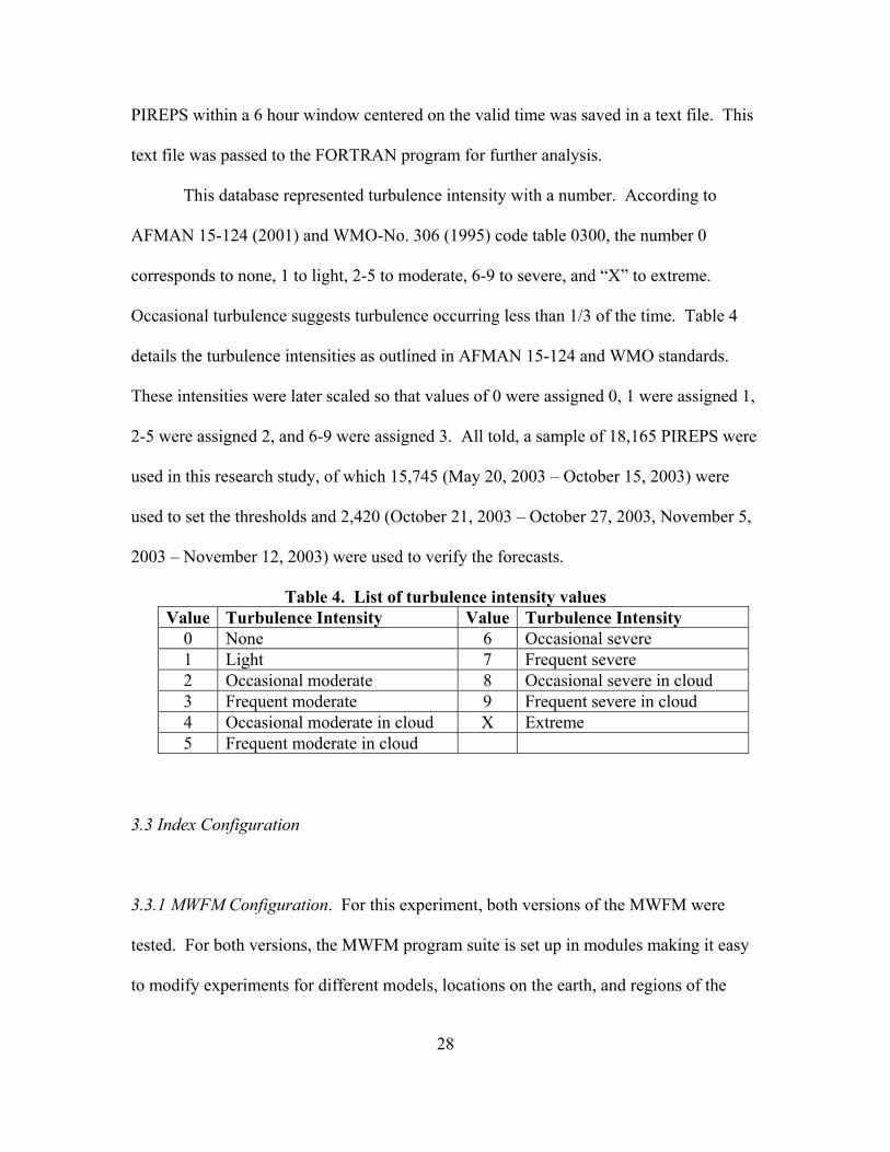
This database represented turbulence intensity with a number. According to

AFMAN 15-124 (2001) and WMO-No. 306 (1995) code table 0300, the number 0

corresponds to none, 1 to light, 2-5 to moderate, 6-9 to severe, and “X” to extreme.

Occasional turbulence suggests turbulence occurring less than 1/3 of the time. Table 4

details the turbulence intensities as outlined in AFMAN 15-124 and WMO standards.

These intensities were later scaled so that values of 0 were assigned 0, 1 were assigned 1,

2-5 were assigned 2, and 6-9 were assigned 3. All told, a sample of 18,165 PIREPS were

used in this research study, of which 15,745 (May 20, 2003 – October 15, 2003) were

used to set the thresholds and 2,420 (October 21, 2003 – October 27, 2003, November 5,

2003 – November 12, 2003) were used to verify the forecasts.

Table 4. List of turbulence intensity values Value Turbulence Intensity Value Turbulence Intensity

0 None 6 Occasional severe 1 Light 7 Frequent severe 2 Occasional moderate 8 Occasional severe in cloud 3 Frequent moderate 9 Frequent severe in cloud 4 Occasional moderate in cloud X Extreme 5 Frequent moderate in cloud

3.3 Index Configuration

3.3.1 MWFM Configuration. For this experiment, both versions of the MWFM were

tested. For both versions, the MWFM program suite is set up in modules making it easy

to modify experiments for different models, locations on the earth, and regions of the

29

atmosphere. In this study the model was run over the entire continental United States

(CONUS) from a window including 20N-60N latitude and 140W-30W longitude. This

window provided diverse topography and a variety of weather conditions to test the

indices.

This study initiated the MWFM from a shell script which passed the necessary

date information to start the program, moved the local archive files to the appropriate

MWFM data directories, chose whether to run “ftpoption” 0 or 2, moved the output to the

appropriate output directory, and ensured all the necessary files were stored in the proper

location. When initiated, the MWFM starts the Interactive Data Language (IDL)

interface. It then immediately calls the at_glider.pro IDL script. This script controls the

forecasting sequence by calling any necessary IDL scripts or FORTRAN programs

depending on several input parameters. Most notably, the at_glider.pro script calls the

what2do file which outlines the experiment and drv_glider.pro which calls the actual

forecast routines.

The what2do file determines where and how the MWFM will run an experiment.

It also outlines how any output will look and what parameters the program should

provide to the user. It is one of several files that must be manipulated to set up a new

experiment. For this experiment, the what2do file, what2do_belsontest.pro, was set up

to run the model over the continental United States (CONUS) for all pressure levels that

comprise the 10,000 ft to 50,000 ft MSL altitude range. The levels and field keyword

were set up to reflect the desire to view the turbulence intensity variable for all the 50

millibar layers between the 800-850 mb layer and the 100-150 mb layer. The latitude and

longitude limits variable was set up to cover 140W to 30W longitude and 20N to 60N

30

latitude. Furthermore, the what2do file was set up to run both V1.1 and V2.1 with GFS

model data as input. For a copy of the what2do file used in this experiment, refer to

Appendix B.

Figure 3. Example of output from MWFM V2.1 The output from MWFM V1.1 and V2.1 was set to save graphical and raw data. The

graphical output was saved in postscript format. It was only used to test the accuracy of

the FORTRAN code which converts the MWFM output to gridded output for display

with the Grid Analysis and Display System (GrADS) software and was not configured

for ideal viewing. An example of the graphical output used for testing is provided in

Figure 3. In Figure 3, the dark region along the California/Nevada border indicates

31

turbulence. Additionally, two scripts saved the raw data with latitude, longitude, and

turbulence intensity for each ridge in the window.

3.3.2 Ellrod-2 Index Configuration. The Ellrod-2 index was implemented with the same

equations used in calculating the index at the Air Force Weather Agency. The equations

used 2nd order centered finite differencing to compute the vertical wind shear (VWS),

convergence (CVG), and deformation (DEF) terms. Using centered differencing when

computing VWS introduces some error since the difference in height between pressure

levels is not constant and the center pressure level is not in the geometric center. This

simplification resulted in an error of 5% or less in the computation. Also, geopotential

height was substituted for geometric height in the computations. According to Holton

(1992), the geometric height and geopotential height are almost identical in the regions of

interest for this study. Computing the index for a level requires the U and V wind data

for three adjacent levels, centered on the desired level. It also required the geopotential

height for the levels directly above and below the desired level. Distances were

calculated using the haversine method, as described by Sinnott (1984). The equations

used in the haversine method are provided in Appendix A and the FORTRAN subroutine

is provided in Appendix E, subroutine Haversine. For the FORTRAN code used to

compute the Ellrod-2 index, refer to Appendix E subroutine Ellrod2.

32

3.4 Implementation

The indices were combined using a series of shell scripts and a FORTRAN

program. The controlling script retrieved the necessary analysis, 12-hour forecast, and

24-hour forecast data files (GFS U, V, and GPH fields, MWFM V1.1 and V2.1 raw data

files, and PIREPS based on the date) required for the FORTRAN program. For each

level, the FORTRAN program computed the Ellrod-2 index with the GFS data fields, the

MWFM with the raw data, the average layer height, and the index value for each pilot

report with the truncated PIREPS text file. The indices were saved to a data file for

display using GrADS software while the PIREPS data was saved to a text file for

statistical study.

The FORTRAN program also created another chart that provided a composite

view of the indices. This chart was designed to provide the forecaster with a snapshot of

the atmosphere from above that would allow them to quickly determine the horizontal

location of the turbulent regions. This information was stored in the same data file as the

other index files.

3.4.1 Index Implementation. The Ellrod-2 index was computed at every available level

between 100 mb and 750 mb. This amounted to 14 levels separated by 50mb each.

Since this computed the index for a specific level and the MWFM computed the index for

a 50 mb layer, it was impossible to make the indices represent the exact same region of

the atmosphere. This problem was addressed by assigning the bottom of the MWFM

layer and the corresponding Ellrod-2 index to the same chart. For example, the 500-550

33

mb MWFM layer and the 550 mb Ellrod-2 level were displayed on the same chart. The

choice was made to display the Ellrod-2 index from 150 mb to 750 mb instead of from

100 mb to 700 mb since the winds at the top of the column are above the troposphere and

typically do not vary as much as the winds in the troposphere.

Additionally, the average geopotential height for each layer was computed. This

computation was performed for each grid point in the model by averaging the height for

two adjacent levels. The results were used as the heights to assign values of each index

to the PIREPS for the MWFM indices. The Ellrod-2 index levels were determined using

the height of the actual level for which the Ellrod-2 index was computed. The PIREPS

assignment scheme is discussed further in Section 3.4.2.

Figure 4. Example of accuracy of MWFM display using GrADS

The MWFM indices were computed for each grid point in the region of interest.

The raw data only contained a subset of latitudes and longitudes for the region that

matched ridges as contained in the MWFM database. This raw data included turbulence

34

intensities greater than 0.0. A representative graphic on the grid was made using the

largest value of the index in a 1° X 1° box centered on each grid point. This ensured that

the maximum value was assigned to every point in the array, guaranteeing the worst-case

is always chosen (a desirable trait where flight safety is concerned). If there were no

values of raw data within that box, the grid point was assigned a value of zero. This

method provided accurate results when compared to the postscript files produced by the

MWFM. Figure 4 provides an example of the comparative output from the MWFM and

the FORTRAN code with MWFM output on the left. The peak magnitudes for the two

images in Figure 4 are located in the same place. Subroutine Mwfm_grid in Appendix E

provides the FORTRAN code used to compute the grid point’s mountain wave values.

3.4.2 PIREP Index Assignment Implementation. To calibrate the index values to

turbulence intensity, pilot report data and the model analyses were used. The PIREPS

were provided by AFCCC for the period of May 20, 2003 to October 15, 2003. A large

file containing all the PIREPS from this period was parsed by a shell script to only

include the PIREPS in a six hour window centered on the valid time of the forecast.

Then, for each pilot report, the levels above and below the PIREPS were determined

based on the level height for the Ellrod-2 index. Finally, the maximum of each index of

the eight grid points surrounding the location of the pilot report were assigned to each

PIREP. This method matched the method used in the Brown et al. (2000) study. Refer to

Appendix E subroutine PR_int for the FORTRAN code used to assign index values to

PIREPS.

35

3.4.3 Composite Index Implementation. The composite index was computed for all the

levels and layers in the study. To determine it, the FORTRAN program computed a

value of 0, 1, 2, or 3 for none, light, moderate, or severe turbulence for each grid point in

the array. Turbulence values were assigned by comparing each index to each threshold,

as described in Section 4.2, for every layer or level. When three adjacent layers or levels

exceeded an index’s threshold, and that grid point had not already been assigned a greater

turbulence value, that grid point was assigned the corresponding turbulence value. For

example, if the 450 mb, 500 mb, and 550 mb Ellrod-2 index values all exceeded the

moderate threshold for a grid point and the grid point had previously been assigned a 0

(none) or 1 (light), the grid point was reassigned a 2 (moderate). If the same grid point

had already been assigned a 3 (severe), it would have remained a 3. Refer to Appendix

E, subroutine Comp_make for the FORTRAN code used to create this chart.

Additionally, the maximum value for each index for each grid point was also computed

and stored in an array. Finally, these four additional fields (composite, max Ellrod-2,

max MWFM V1.1, and max MWFM V2.1) were stored at the end of the data file with

the individual indices for display using GrADS software.

3.4.4 GrADS Implementation. GrADS software was used to make the necessary image

files for the forecaster graphics. GrADS works with unformatted FORTRAN data stored

in four dimensions very easily (longitude, latitude, height, time). The data files created

by this FORTRAN program saved the index values in three dimensions (longitude,

latitude, height). The longitude array elements were stored from 140W-30W and the

latitude array elements were stored from 20N-60N. The height elements were stored

36

such that the layers from 100-150 mb to 700-750 mb of the MWFM indices corresponded

to the levels from 150 mb to 750 mb for the Ellrod-2 index. The composite layer was

stored as an additional height layer after the bottom layer in the array. GrADS relies on

metadata files to tell it how to interpret the data it reads. GrADS also has a scripting

feature to string together a sequence of commands. The metadata file and script used to

generate the imagery are provided in Appendix C. Information on using GrADS was

obtained from on-line documentation (GrADS 2003).

Figure 5. Example composite chart

For viewing the data, the indices were contoured on a map of the CONUS. The

contours were determined by the thresholds as determined by the PIREP data. The

threshold values, as determined in Section 4.2, were 2.16, 3.00, and 8.37 for the Ellrod-2

37

index, 0.00033, 0.00140, and undefined for MWFM V1.1 index, and 0.012, 0.020, and

0.036 for the MWFM V2.1 index. The charts developed by GrADS were saved in “Joint

Photographic Experts Group” (JPEG) format.

To reduce the work required by the forecaster, a composite image was created

from the composite index. This image shaded each respective threshold with values of 2

and 3 being depicted as gray shades in Figure 5. In Figure 5, regions of moderate

turbulence are shaded lighter than regions of severe turbulence and are described in

Section 3.4.3. The intent was to allow the forecaster to trace the regions outlined by the

composite chart and use the layer viewer to determine the levels of the atmosphere that

indicate the potential for CAT. This image was saved in JPEG format also.

3.4.5 Turbulence Layer Viewer Implementation. The turbulence layer viewer provided a

quick method of interrogating the atmosphere and determining the turbulent levels.

Because of the relatively large size an image must be to properly interrogate it with a

computer, forecasters are ordinarily limited to examining each layer individually. The

layer viewer circumvents that problem by allowing forecasters to view the same portion

of several layers of the atmosphere at the same time.

The layer viewer requires frames and javascript to work and was designed to

work with the Microsoft® Internet Explorer V6.0 web browser. It is composed of two

primary areas. The first area holds the layers. To speed up the transition between layers,

the viewer immediately loads all the available layers into memory despite only displaying

a few of them. In this study, four layers of the 14 were displayed in the first area but that

number could be easily modified. The second primary area holds the two tools needed

38

to control the layers. The first tool is the up/down buttons. Clicking on either of these

buttons shifts the four displayed layers up or down by one layer. The other tool is a

vertical scrollbar. Because of the viewing size of the four images, only a portion of each

image in the first area display region is viewable at a time. Adjusting the scrollbar shifts

the viewable region in each window of the first area display region to the same place.

This feature may not work properly with a Netscape® browser or older Internet Explorer

versions. The images used in this study did not require a horizontal scrollbar. If a

horizontal scrollbar were required, a few simple modifications of the javascript used by

the vertical scrollbar are all that would be required. Refer to Figure 6 for an example of

the layer viewer and Appendix D for a summary of the html and javascript code used in

making the layer viewer.

Figure 6. Turbulence layer viewer

39

Aside from the two primary areas, additional areas provide an approximate flight

level for each layer and a title. The approximate flight level was calculated for layers

below the tropopause layer using equations 14 and 15.

0

0

1dRgT pz

p

Γ = − Γ

(14)

1 2

2layer layer

avg

z zz

+= (15)

Equation 14 is based on the U.S. Standard Atmosphere below the approximate

tropopause (8 km or about the 200-250 mb layer). In this equation, z is the height, dR is

the dry air gas constant 287.04 1 1J kg K− −⋅ ⋅ , T is the average temperature 288.15 K, g is

the acceleration due to gravity 9.80665 2m s−⋅ , 0p is the reference pressure 1000 mb, and

p is the pressure at the level of interest. Equation 15 averages the height for the top and

bottom level of each layer.

Table 5. List of flight levels based on pressure Layer Flight Level Layer Flight Level

0 100-150 mb FL480 450-500 mb FL2000 150-200 mb FL420 500-550 mb FL1700 200-250 mb FL360 550-600 mb FL1500 250-300 mb FL320 600-650 mb FL1300 300-350 mb FL280 650-700 mb FL1100 350-400 mb FL250 700-750 mb FL0900 400-450 mb FL2200

For each of the layers, the height was verified with a sample of the model output.

Additional comparison was performed visually with a skew-T of the U.S. standard

40

atmosphere. It is important to remember these heights are estimates of the heights in the

atmosphere and are to be used as a guide. The values determined using these methods

are presented in Table 5.

The region of the atmosphere chosen for the upper level turbulence charts poses a

concern to this method of height determination. When flying at or above FL180, aviators

set their altimeter to the standard surface pressure, 29.92 inches Hg. When flying below

FL180, aviators use a nearby station pressure (FAA 2003). This difference in altimeter

settings can produce differences in indicated altitude of several hundred feet. For the

purpose of this study, the potential difference in altitude was considered as a possible

source for error but no efforts were made to account for it since the charts assign a region

of altitudes as potentially turbulent levels and not specific heights.

The data file containing the three index values and composite data was used to

populate the turbulence layer viewer. The images were generated using GrADS scripts as

described in section 3.4.4.

3.5 Turbulence Chart Methodology

After determining the thresholds, the test method was verified using PIREPS.

Producing the turbulence charts with the test method required two steps. First, depending

on the desired minimum turbulence, the contour indicating the desired turbulence

intensity was outlined. For this study, MOG turbulence intensity was chosen since as a

matter of practice, weather squadrons only forecast regions of moderate or greater

turbulence. When two or more areas suggesting MOG turbulence were very close

41

together, one circle encompassing all the areas was drawn. Second, using the layer

viewer, the altitudes where turbulence was present were located and the circled regions

on the map were labeled with the estimated base and top of suspected turbulence. This

occasionally required dividing large outlined regions into parts to make a more

representative visualization.

Despite every attempt to make a purely objective forecast tool, several aspects of

this method required forecaster subjectivity. First, when two or more areas on the

composite chart suggesting MOG turbulence were very close together, one circle

encompassing all the areas was drawn. This improved the appearance of the charts but

required the forecaster to determine when two regions were close enough to be joined.

Second, there were several situations that often arose when using the layer viewer which

required some interpretation. First, within a layer, different intensities were present

within one of the highlighted regions. In general, the level was included if more than half

of the layer contained any indication of turbulence with at least some of that meeting the

moderate or greater threshold. The other situation involved interpreting between two or

more levels. Occasionally, two levels which obviously needed to be included were

divided by a layer that appeared less likely to contain turbulence. In this instance, any

indication of moderate or greater turbulence by the intermediate layer led to inclusion of

that altitude. Furthermore, the top or bottom of the turbulent region rarely stopped on a

layer exactly. Determining the actual heights of the top and bottom required some

interpretation by the forecaster. All of the subjective decisions were made as a matter of

practicality and are similar in practice to steps used by USAF weather forecasters to

42

estimate heights and regions of turbulence. These simplifications allow the aviators and

mission planners to review a usable, easily readable turbulence chart.

Verification of charts produced by the test method and the weather squadrons

were also done using the same PIREPS database. The results of both methods using the

statistics discussed in Section 3.6.2 are detailed in Chapter 4.

3.6 Statistical Methods

The statistical analysis performed during this research can be divided into two

primary parts. First, the thresholds for each of the three indices needed to be determined.

This was done to provide a basis for the forecast tools. The primary goal of this stage

was to determine usable values of each index that correspond with light, moderate, and

severe turbulence. These thresholds were then used to create the images used by the

turbulence viewer software to assist the forecaster in turbulence chart development. The

second stage of the statistical analysis involved verifying forecasts produced using the

test method with PIREPS and comparing it to verification of actual forecasts produced by

USAF weather squadrons.

3.6.1 Threshold Determination. The thresholds were determined with a FORTRAN

program which processed every possible combination of indices looking for the ideal

combination based on contingency table statistics as described in Table 1. Several

different criterion were compared to determine the thresholds including the PODy

maximum, PODn maximum, FAR minimum, CSI maximum, PC maximum, TSS

43

maximum, closest BIAS score to one, the first instance when PODy was less than or

equal to PODn, the maximum HSS, and the maximum GSS.

The HSS and GSS are statistics developed to determine the actual skill of a

forecast relative to random forecasts. According to Wilks (1995), the HSS is the most

common skill score used to summarize square contingency tables. It essentially

compares the forecasts to a generic reference forecast, using the equation in Table 1, with

the same marginal distributions of forecasts and observations as the actual contingency

table. The HSS returns a value less than or equal to one. A score of one signifies a

perfect forecast while forecasts worse than the generic reference forecast receive scores

less than zero. Schaefer (1990), describes the GSS as the CSI corrected for the number of

hits expected by chance. A perfect forecast receives a score of one. The closer a

forecast is to being purely random, the closer the GSS will be to zero (Stephenson 2000).

The equations used in calculating the HSS and GSS are listed in Table 1.

The FORTRAN program contained four nested loops. The loops cycled through

every combination of the three indices over user-determined ranges of values at user-

determined increments. Additionally, the program could be configured to analyze

different flight levels, turbulence intensities, latitude/longitude ranges, and different

lengths of time centered on the forecast hour for the same statistics. After computing the

statistics, the FORTRAN program saved the results to an output file for review.

After determining the thresholds, the χ2 test, as described in Montgomery and

Runger (2003), was performed on the contingency tables to test for independence. In this

test, the null hypothesis was that forecasts were independent of observations. An alpha of

0.05 was used to reject the null hypothesis and determine whether forecasts and

44

observations of turbulence were dependent on each other. The test statistic in a χ2 test is

computed using the equation:

2

2 ( )ij ij

i j ij

O EE

χ−

=∑∑ (16)

where ijO is the observed contingency table values, ijE is the expected table values, and i

and j are the rows and columns. The observed contingency table is the contingency table

calculated from the data while the expected contingency table is computed using:

( )i j

ij

tot totE

total= (17)

where itot represents the total of row i in the observed contingency table, jtot is the total

of column j in the observed contingency table, and total is the sum of all the cells in the

observed contingency table. After determining the χ2 value for the data, it was compared

to the table value of χ2 for an alpha of 0.05 with 1 degree of freedom or 3.84. If the

computed χ2 value exceeded 3.84, the null hypothesis was rejected.

3.6.2 PIREP Verification. After the thresholds were determined, the layer viewer

software was configured with the thresholds to allow for forecasts to be developed.

These forecasts were made over the CONUS from October 21, 2003 to October 27, 2003

and from November 5, 2003 to November 11, 2003. Contingency tables combining

PIREPS and forecasts were used to compute the same statistics discussed in section 3.6.1.

Additionally, forecasts produced by USAF weather squadrons over the CONUS for the

same dates were verified using the same methods. The USAF weather squadron forecasts

originated from stitched charts produced by the 26th OWS at Barksdale AFB. These

45

stitched charts represented the combined forecasts of turbulence charts produced by the

15th OWS at Scott AFB, 25th OWS at Davis-Monthan AFB, 26th OWS at Barksdale AFB,

and 28th OWS at Shaw AFB.

46

IV. Results

4.1. Introduction

This chapter summarizes the results from the various contingency table analyses

performed using the PIREPS and the various forecasts. It begins with a discussion of the

various analyses performed on the data to determine the different thresholds. This

includes testing for whether the thresholds vary by altitude or geographic region. It also

includes testing the thresholds for turbulence greater than or equal to light, greater than or

equal to moderate, and greater than or equal to severe. After completing the threshold

determination, the established thresholds were entered into the FORTRAN program that

computed the indices and the program was rerun to generate the products used by the test

forecast method. The second section describes the results of the forecast comparison

between the test method and operational forecasts. It focuses on the relative accuracy of

the test method to the forecasts currently produced by the various weather squadrons.

4.2. Threshold Determination

Thresholds were determined using the subset of PIREPS within six hours of the

model analysis runs from May 20, 2003 to October 15,2003. For example, for a model

forecast valid at 12Z, any PIREP between 0900 and 1459 were used. Using this subset of

PIREPS provided a sample size of 15,745. In determining the thresholds, the Ellrod-2

index threshold was found for each intensity level first. This was done by setting the

47

ranges for the MWFM indices with a value of 99.0. This value was well outside of

maximum value of either MWFM index. After determining this threshold, the MWFM

V2.1 threshold was found with the Ellrod-2 index set to its already determined threshold.

Finally, the MWFM V1.1 threshold was found with the other two indices set to their

established thresholds. This order of threshold determination was chosen because the

MWFM V1.1 threshold tends to contain output for the region directly above a ridge while

MWFM V2.1 propagates energy downstream making it provide output over larger

regions of the map. The order intended to ensure the best chance that each index

contributed to finding positive reports of turbulence the other indices, covering larger

areas, missed. The criteria most often used to set the thresholds included the skill scores

and the point where PODy crossed PODn. The results of threshold determination are

provided in Table 6.

Table 6. Thresholds determined for indices

Chart Index TH PODy PODn TH PODy PODn TH PODy PODnLayers Ellrod 2 2.16 0.50 0.63 3.00 0.45 0.67 8.37 0.21 0.94

MWFM V1 0.00033 0.67 0.49 0.0014 0.56 0.60 - - -MWFM V2 0.012 0.66 0.49 0.02000 0.54 0.61 0.03600 0.33 0.87

Light Moderate Severe

From Table 6, the light and moderate thresholds were quite close to each other for

each of the indices. This would make separating regions of light and moderate

turbulence difficult. Since Air Force weather squadrons only predict regions of moderate

or greater turbulence in practice, this problem should not have significantly affected the

skill of the test forecast method.

Threshold determination also provided several noteworthy results not listed in

Table 6. First, there were only 24 instances of severe turbulence in this sample making

48

determination of the thresholds for that intensity unreliable. This led to the establishment

of an almost arbitrary value for the severe turbulence thresholds and no value being

determined for the MWFM V1.1 index severe threshold. As such, any indication of

severe turbulence by the forecast method was ignored for this study and only moderate

regions were highlighted for the verification study of Section 4.3. Additionally, the χ2

test was performed on the contingency table produced by the combined thresholds for

moderate turbulence. The resulting value of 193.5323 suggested there was a 5.39x10-42%

chance of incorrectly rejecting the null hypothesis with this χ2 value. This provided

strong evidence to reject the null hypothesis and conclude the index values offer some

skill in predicting turbulence. Another interesting fact of this test was that FAR did not

increase with the addition of MWFM indices to the forecast. In fact FAR decreased from

0.8394 to 0.8339 to 0.8338 as the MWFM indices were added to Ellrod-2 index when

computing the moderate layer threshold. This provides another indication that the

MWFM indices improve the forecast. Additionally, the MWFM indices provide a larger

improvement in the PODy than the degradation in the PODn, suggesting they add value

to the forecast.

After determining the thresholds, it was necessary to see if they change

significantly for different geographic regions or altitudes. This test was performed by

setting the indices to the established thresholds and calculating the statistics over different

regions or altitudes. For this test, there were nine different regions tested for moderate

turbulence. The regions included the following areas: A) Entire region, B) FL100-

FL200, C) FL200-FL300, D) FL300-FL400, E) FL400-FL500, F) 110W-70W and 20N-

40N, G) 110W-70W and 40N-60N, H) 70W-30W and 20N-40N, and I) 70W-30W and

49

40N-60N. The resulting statistics are listed in Table 7. The statistics varied considerably

for different regions and levels in the atmosphere suggesting different thresholds based

on geographic region or altitude might produce more accurate results. In addition,

several of these samples failed the χ2 test for independence. Those tests include E, H, and

I with χ2 values of 2.00, 1.38, and 3.44 respectively. Each of these χ2 values, with an α of

0.05, fail to reject the null hypothesis. In test H, the “yes/yes” cell only expected 1.62

occurrences. According to Wilks (1995), cells containing less than five instances of an

expected event should be avoided. Also, in tests H and I, there were only 13 and 35

positive reports of moderate or greater turbulence. This lack of positive reports decreased

the credibility of the statistics listed for those rows. Despite the lack of validity regarding

these two regions, there does appear to be some regional variation in the thresholds.

Table 7. Statistics for different regions

TestSample

Size PODy PODn FAR CSI PC BIAS TSS HSS GSSA 15745 0.5628 0.5983 0.8225 0.1560 0.5935 3.1703 0.1611 0.0840 0.0438B 2136 0.5367 0.6001 0.6004 0.2971 0.5791 1.3432 0.1369 0.1260 0.0672C 1161 0.6187 0.5102 0.6240 0.3053 0.5452 1.6453 0.1288 0.1102 0.0583D 11987 0.5696 0.6030 0.8911 0.1006 0.6004 5.2295 0.1726 0.0588 0.0303E 463 0.4487 0.6364 0.8000 0.1606 0.6048 2.2436 0.0851 0.0569 0.0293F 4837 0.5555 0.6466 0.6498 0.2735 0.6233 1.5862 0.2021 0.1694 0.0925G 4922 0.5822 0.5503 0.7913 0.1815 0.5557 2.7899 0.1325 0.0774 0.0402H 869 0.2308 0.8773 0.9722 0.0254 0.8677 8.3077 0.1081 0.0235 0.0119I 5167 0.6000 0.5563 0.9909 0.0091 0.5566 65.6571 0.1563 0.0047 0.0024

4.3 Forecast Comparison

To compare forecast skill, 12-hour and 24-hour forecasts were made using the test

method and verified with PIREPS. Additionally, 12-hour and 24-hour operational

forecasts produced by the Air Force were also verified with PIREPS. When initially

50

attempting to implement the test method as an operational forecast tool, the indices

produced output that was very confusing and that would have been difficult to use

operationally. The composite images produced with these thresholds were very

congested with contours, as depicted by the image on the left in Figure 7. As a result, the

composite image only depicted regions with turbulence when three adjacent layers

indicated turbulence at a grid point as described in section 3.4.3. This modification

produced the image on the right in Figure 7 which was much easier to contour.

Figure 7. Examples of composite level output

After adjusting the method for computing the composite chart, forecasts were

made using the test method. Typically, these hand-plotted forecasts took less than five

minutes to produce. Next, these test forecasts and actual forecasts produced by

operational weather squadrons were verified for accuracy with PIREPS from October 21,

2003 to October 27, 2003 and from November 5, 2003 to November 12, 2003. To verify,

PIREPS were compared by location and height to the forecasts. In order to be counted,

PIREPS needed to be above the CONUS since the weather squadrons did not forecast

51

outside the CONUS. When a PIREP fell within a region highlighted to suggest

turbulence, it was considered forecasted. Only PIREPS of moderate or greater intensity

were considered observed.

The PIREPS were plotted using GrADS on a chart that contained the test method

forecast regions so the comparison was quite accurate for the test method. Operational

forecasts were compared with PIREPS using estimation. To ensure the weather squadron

forecast skill was maximized, PIREPS appearing very close to a region of forecasted

turbulence were given the benefit of the doubt. In general, these events were scored as

either “yes/yes” or “no/no”. Furthermore, this study only predicted regions of moderate

or greater turbulence. There were many PIREPS of light turbulence reported in

forecasted regions of moderate turbulence. Those regions were scored as forecasted

“yes” but observed “no” or “yes/no”. The test method and operational forecast

contingency tables are provided in tables 8 and 9. The χ2 test scores of 189.9 for the test

method and 35.97 for the operational forecasts are sufficient to reject the null hypothesis

leading to the conclusion that forecasts and observations are not independent.

Table 8. Test method contingency table Table 9. OWS forecast contingency table

Yes NoForecasted

Yes

No 246 1371

Observed

325 478

Yes NoForecasted

Yes

No 484 1719

Observed

87 130

52

These tables suggest significant differences exist in the two methods. In general,

the operational forecasts tend to significantly under forecast turbulence event relative to

the test method, as evidenced by the large number in the “no/yes” cell. At the same time,

the test method appears to significantly over forecast turbulence. This apparent weakness

is tempered by the short-lived nature of CAT and the low reliability of the “yes/no” cell

as a determinant of forecast skill. Also, negative reports of turbulence would often

appear very close to positive reports of turbulence in time and location further validating

the claim that CAT is short-lived and localized. Also, the operational forecasts did not

appear to consider turbulence caused by mountain waves. There was not one region

depicted on the charts over these two weeks where the weather squadrons used solid blue

lines to depict mountain wave turbulence. This may be due to mislabeling since there

were several regions which suggested the forecaster considered the turbulence to be

mountain wave turbulence although they used the general CAT line style to circle them.

Table 10. Verification statistics PODy PODn FAR CSI PC BIAS TSS HSS GSS

Test Method 0.569 0.741 0.595 0.310 0.701 1.406 0.311 0.272 0.231Operational Forecasts 0.152 0.930 0.599 0.124 0.746 0.380 0.082 0.104 0.114

Instances where the test method did not forecast regions that observed turbulence

were explored further to determine the cause. There were several possible reasons the

test method did not highlight these regions of turbulence. Several observed instances of

turbulence appear to have been caused by convection. These instances would not meet

the definition of CAT but were left in the tables since this is a comparative study of

53

forecast methods and, in general, neither method forecasted those regions. The most

common cause of missed regions of turbulence was near misses where the turbulence

appeared just outside of the highlighted areas. Many of these near misses were captured

with the actual layer viewer. Table 10 provides the detailed breakdown of the statistics

produced from the contingency tables for the test method and operational forecasts.

The test method appears superior to operational forecasts. The test method scored

significantly higher PODy, TSS, HSS, and GSS over the operational forecasts. The

higher PODn of the operational forecasts is due in large part to the significantly lower

volume coverage of the forecasts. The bias scores suggest the test method tends to over-

forecast turbulence while the operational forecast tends to under-forecast turbulence.

However, the test method bias is closer to one suggesting it tends to over-forecast less

than the operational forecast tends to under-forecast.

54

V. Conclusions and Recommendations

5.1 Conclusions

For many years, meteorologists have attempted to predict occurrences of clear-air

turbulence. In recent years, various numerical indices have been developed and tested to

quantitatively predict CAT. It had been shown that numerical models outperform

conceptual models when forecasting CAT (Dutton 1980). This study seems to back up

that assertion. This research focused on developing a new technique for predicting CAT

that incorporated three numerical model indices, the Ellrod-2 index and the two MWFM

indices. Including tools for predicting both primary causes of CAT provided a

comprehensive prediction method. The technique was developed to meet the needs of

Air Force operational weather squadron forecasters for a comprehensive, easy-to-use

automated forecast method. Furthermore, the technique is adaptable to indices other than

those chosen in this study.

The mountain wave forecast model indices showed promise in predicting CAT

regions in the troposphere. The V2.1 index provides more comprehensive coverage than

the V1.1 index. However, MWFM V2.1 does not appear to capture every region of

mountain wave turbulence, and the V1.1 index appears to add some value to the overall

forecast. Although most turbulence encounters appear to be represented by an index

depicting Kelvin-Helmholtz instabilities, there were several instances that the MWFM

captured but that the Ellrod-2 index missed. In this study, the mountain wave indices

55

appeared to capture about one in every ten correctly forecasted moderate or greater

turbulence encounters throughout the column, not just near the tropopause.

The test method appears to provide superior forecasts to those currently produced

by the operational weather squadrons who appear to primarily use conceptual models in

their turbulence chart development. This is most likely the cause of the significant under-

forecasting and inaccuracy in the weather squadron products used for this research.

While the test method provided a large number of near misses on occurrences of

turbulence, PIREPS of turbulence were often quite far from the nearest turbulent region

indicated by the weather squadron forecasts. However, the test method charts tend to

encompass a large portion of the atmosphere making turbulent conditions appear quite

widespread. Furthermore, the test method appears to miss quite a few instances of

turbulence despite the layer viewer depicting those regions as turbulent. These misses are

caused by the implementation of the composite chart as described in Section 3.4.3. Also,

because of the significant coverage of turbulent regions by the test method, using the test

method is not as straightforward as initially thought. This was especially true over the

Rocky Mountains as they often have numerous levels and layers where the mountain

wave forecast models predicted turbulence.

This study only focused on moderate or greater turbulence. The length of time

used in this study did not provide an adequate number of severe PIREPS (due to their

limited availability) to properly threshold severe turbulence events. The few instances of

severe turbulence actually depicted in this study did allow for some degree of threshold

determination; however, the results are unreliable and, therefore, deemed inconclusive.

Properly thresholding severe turbulence would require a much longer test period,

56

encompassing many more severe turbulence encounters than identified in the sample

analysis.

Overall, the test method appears to offer promise as a tool that simplifies an

otherwise complex process. The time required to develop forecasts for the CONUS using

this new tool should be less than five minutes per forecast hour shortly after the

forecaster masters the technique and the OPS II drawing features. Furthermore, the

largely objective nature of the method will reduce the inconsistency between forecasters

and lessen the impact of inexperience on the reliability of the product.

Although this method was developed for turbulence, similar techniques using a

composite chart and layer viewer may provide additional benefits in other areas of

forecasting such as for aircraft icing. Additionally, the layer viewer can be used to aid

the forecaster in synoptic scale analysis and forecasting.

5.2 Recommendations

5.2.1 Recommendations to AFWA and 15th OWS. This method appears to offer a

superior, comprehensive tool in developing upper level turbulence charts. It allows a

large portion of the globe to be quickly analyzed for turbulence. Furthermore, a method

very similar to the test method has been used operationally at the 17th OWS for over two

years. The OPS II script employed by the 17th OWS generates a composite chart and

layer viewer charts very similar to those developed for this study. However, the script

used at the 17th OWS does not include mountain wave turbulence and only used output

from two adjacent layers instead of the three layers used in this study.

57

It is strongly recommended AFWA run the mountain wave forecast model V1.1

and V2.1 for the troposphere and converts that output into a format suitable for use by

OPS II. If it is necessary to make the data match gridded output, it is suggested AFWA

use the same approach employed in this study. Furthermore, the layer viewer html and

javascript code should be provided to the operational weather squadrons for their

immediate implementation. The code developed for this method can be easily modified

by the weather squadron web masters and used to supplement or replace current

techniques.

Finally, to better meet the needs of aircrews, it is recommended that weather

packages include the traditional turbulence chart, as generated by the test method, along

with several layer-specific charts based on unanalyzed model output near the flight level

of the aircraft. This provides the pilot with a general idea of the turbulent regions, as well

as, the areas of potential turbulence at the levels they are flying. Providing both charts

will offer the most complete picture of where the aircrew might experience turbulence

and what their best course of action might be to avoid the turbulence if necessary.

5.2.2 Future Research Recommendations. There are numerous additional research

studies that may be performed to further test the methods developed here. The test

performed in Table 7 suggests the indices’ thresholds may vary based on levels of the

atmosphere and geographical locations of the aircraft. Additional studies to determine if

the thresholds vary based on those criteria might be performed. Furthermore, this study

used GFS model data to determine the Ellrod-2 index and initialize the mountain wave

58

forecast model. Using higher resolution model data might provide more accurate results

than using the data chosen here.

This study focused on determining regions of moderate turbulence using data over

a five month period to calibrate the indices. Additionally, the study only verified

forecasts for two weeks in the fall. This limited study was adequate to demonstrate the

relative skill of the test method to operational forecasts but further studies using a larger

dataset might allow accurate calibration of severe turbulence thresholds and it might

provide insight into how the index thresholds change with different seasons. Future

studies might also use PIREPS that include aircraft type to more accurately assess

intensity reports. Also, no steps were taken to initialize or verify the GFS model using to

compute the indices before making the forecasts. Taking those steps might further

increase the accuracy of the forecast method.

This study only tested three indices in predicting CAT, using the Ellrod-2

turbulence index as a means of determining CAT caused by Kelvin-Helmholtz

instabilities. There are many other indices developed to predict CAT caused by Kelvin-

Helmholtz instabilities. Future studies might consider using a different index or using an

ensemble forecast of sorts with several different indices to determine if they provide

more accurate results. These ensembles might rely on several indices on a layer

indicating turbulence as opposed to this study’s reliance on several different layers

depicting turbulence to mark an area with turbulence. Additionally, future versions of the

MWFM or other mountain wave models might become available that would require

testing to determine their use.

59

Finally, this method is a step towards completely automating the CAT product

produced by weather squadrons. It seems a similar method using sets of rules could be

developed to produce a chart without any forecaster involvement at all. This method

might reduce the forecaster’s role to quality control checking the chart and adjusting

regions based on model error in initialization or verification purposes only. This would

further simplify the CAT forecast process and essentially eliminate the forecaster from

being in the loop for CAT prediction altogether.

60

Appendix A: Detailed Computations

1. Computations involved in MWFM V1.1 (Bacmeister et al. 1993). This is designed to provide a basic understanding of the underlying equations involved in computing turbulence with the Mountain Wave Forecast Model.

First, the local saturation limit is computed ;

;

( )( )

( )k

sat kk

U zz

N zδ ⊥=

Then, a first guess of the wave displacement profile at a level is made using

1/ 2

;*

;

( ) ( ) ( )( ) ( )

( ) ( ) ( )k k

k kk k

z N z U zz z z

z z N z z U z zρ

δ δρ

⊥

⊥

+ ∆ = + ∆ + ∆ + ∆

If this value is more than the saturation limit, it is reduced to the saturation limit. To compute the value at the surface, use the minimum of saturation value at the surface and 4 ka where ka is a ridge height parameter. Now, the momentum flux is approximated by

2

;( )( ) ( ) ( ) ( ) k

k k kzz z N z U z

Lδφ αρ ⊥≈

and this is used to compute turbulence by

2

( ) ( )Turbulence k kz

zKE z z zφ φ∆+ ∝ − + ∆

The definition of the terms: ;sat kδ local saturation limit of wave-induced vertical displacement ;kU ⊥ perpendicular wind component to the ridge based on height kN Brünt-Väisala frequency *

kδ first guess of wave-induced vertical displacement at a level ρ density of the air at a level α dimensionless ridge-shape factor

L horizontal length representing extent of wave disturbance kφ average momentum flux at level k TurbulenceKE The turbulence produced by waves from lost momentum flux

61

2. Haversine method used to calculate distances on this sphere. Method as presented in Sinnott (1984) used extensively to calculate distances. Function passes two sets of latitude and longitudes and returns the distance between them.

2 1 2 1

2 2

1 2sin cos( ) cos( )sin2 2

2arctan1

_

lat lon

lat lon

d lat lat d lon lon

d da lat lat

aca

dist earth radius c

= − = −

= +

= −

= ×

62

Appendix B: CONUS what2do Script

This is the what2do script used by this research to run the MWFM V1.1 and V2.1.

The what2do files are located in the /MWFM/source/jobs/what2do/ directory. Its primary

function is to set up the variables which control how the experiment runs. To run a new

experiment, one must modify several other scripts including:

1. /MWFM/source/jobs/what2do/special_cases.pro: set up a new special case with this number by copying and pasting another special case and modifying it as needed.

2. /MWFM/source/jobs/progs/at_glider.pro: add new special case.

3. /MWFM/source/jobs/drivers/drv_glider.pro: add new special case.

4. /MWFM/source/core/frcst_mtnwave.pro: add new special case.

PRO WHAT2DO_BELSONTEST,date=date,pole=pole,xrang=xrang $ ,field=field,levels=levels,latlonlims=latlonlims $ ,what=what,source=source,grid=grid $ ,sequence=sequence,special=special $ ,psfile=psfile,mwfmversion=mwfmversion $ ,srcplane=srcplane,strict18=strict18,map_ann=map_ann $ $ ,plot_items=plot_items ;+ ; ================================= ; | ( ) ( | ; | M ) W ( F ) M | ; | ( ) ( | ; | _____/^\_____/^\_____/^\_____ | ; | Mountain Wave Forecast Model | ; ~~~~~~~~~~~~~~~~~~~~~~~~~~~~~ ; ------------------- ; WHAT2DO_BELSONTEST ; ------------------- ; template what2do_xxxx.pro routine to set up a new MWFM experiment: replace ; "xxxx" with your experiment name and change various what.* values below to ; tune to your specific experiment, then set up your own drv_xxxx.pro ; (MWFM 1.*) or specialcase in special_cases.pro (MWFM 2.*). ;

63

; ------------------- ; MWFM USAGE e.g., special_cases.pro (source/jobs/what2do) ; LOCATION source/jobs/what2do ; ; ------------------- ; HISTORY ; 20020811 SDE: created as a standardized what2do template from cleaned, ; commented, and documented what2do_usarayforecast.pro ; ; ------------------- ; KEYWORDS/PARAMETERS ; ; date input of standard character date in YYMMDD or YYMMDDZZ ; format: gets plugged into what.date. You should always ; pass a date, otherwise you'll get an unsatsifactory ; default ; pole 2-element vector of the "map pole" or center of the map, ; in the format [longitude,latitude]. If not input, uses a ; default value set below: gets plugged into what.pole ; xrang 2-element x range vector for GSFC map sizing, used ; explicitly only for map_source=0. For new IDL maps it ; is only used unless the (much preferred) explicit sizing ; option "platlonlims" in the pltrec structure (i.e., ; pltrec.platlonlims) is not set. If not input, uses a ; default value set below: gets plugged into what.xrang ; field multi-element vector (# elements corresponding to the ; number of requested forecast plots), containing integer ; MWFM wave field indicies corresponding to various MWFM ; output fields that can be calculated. Type ; FIELD_STRINGS, /LIST within MWFM to see currently ; supported list of permitted wave field indices and what ; they correspond to. If not input, field is set to ; default values set below: field gets plugged into ; what.field ; levels a multi-element vector of exactly the same size as field ; that represents the integer index values of the pressure ; at which you wish to do this forecast. This is dependent ; on the pressure level array of your particular atmospheric ; data source: MWFM has pressures that go from largest ; (low altitude) to smallest (highest altitude), so that if ; the pressure level array is [1000.0,925.0,850.0,700.0....] ; then level=[0,1,3] tells MWFM to plot 3 forecasts: first ; on the 1000hPa surface, second on the 925hPa surface and ; the third on the 700hPa surface. The field plotted in ; each case is given by the field array above: e.g.,

64

; field=[0,0,0] will plot peak vertical displacements in ; each case. To find out allowable pressure surfaces, you ; will need to read your data in using get_glbdata.pro and ; then print out the returned plev array. If not input, ; levels is set to default values set below: levels gets ; plugged into what.levels ; latlonlims a 4-element array that defines the regional ; longitude-latitude bounds [lonmin,lonmax,latmin,latmax] ; within which MWFM will do the forecast. For example, ; latlonlims=[-10.0,30.0,60.0,70.0] performs a forecast ; in the longitude range 10W to 30E and for latitudes ; between 60N and 70N, which corresponds roughly to ; Scandinavia. See get_glbdata.pro for more ; information/context. If not input, latlonlims is set to ; default values set below: latlonlims gets plugged into ; what.latlonlims ; what the output "what2do" structure that this routine returns, ; containing all the information and swtiches needed to ; run this particular MWFM forecast/analysis run just the ; way the user wants. See the structure assignment ; statement below for all the information within it and ; what it all means, or else type HELP, what, /STRUCTURES ; after calling this routine using what=what ; source specify the source string: type GET_GLBDATA,/LIST to get ; listing of currently supported atmospheric data sources. ; e.g., source='NMC' specifies NCEP/NMC data. If not input, ; source is set to default values set below: source gets ; plugged into what.source ; grid the grid string in GSFC format: e.g., 'GG2%5X2%5' for 2.5x ; 2.5 degree lon-lat gridding in the file. Gets plugged into ; what.grid ; sequence the sequence data string in GSFC format, e.g., 'E01' ; special the special data string in GSFC format, again identifying ; the specfic kind of atmospheric data file we're reading ; psfile if set true, activates postscript output via what.psfile=1 ; mwfmversion passes the MWFM version (1, 2, ....) ; srcplane string used to signify the source of aircraft data to be ; overplotted (e.g., 'ER2') ; strict18 older keyword in which atmospheric data at 18 standard ; pressure levels is strictly enforced. If press=-1 ; then it requires data at all X levels (I think) ; map_ann older map annotation keyword ; plot_items another plot annotation device, this time a structure ; used to annote something to a plot. For a sample, see ; code in what2do_solve.pro

65

; ;- ;*********************************** ;AUTHORIZATION TO USE AND DISTRIBUTE ;*********************************** ;I hereby agree to the following terms governing the use and redistribution of ;The NRL Mountain Wave Forecast Model (MWFM), mountain wave forecasting ;and display software, written and developed by Stephen D. Eckermann and ;colleagues at Code 7646 at the Naval Research Laboratory in Washington, DC. ; ;Redistribution and use in source and binary forms, with or without ;modification, are permitted provided that: (1) source code distributions ;retain this paragraph in its entirety, (2) distributions including binary ;code include this paragraph in its entirety in the documentation or other ;materials provided with the distribution, and (3) all advertising materials ;mentioning features or use of this software display the following ;acknowledgment: "This product includes software written ;and developed by Stephen D. Eckermann and colleagues of the Naval ;Research Laboratory (NRL)." Neither the name of NRL or its contributors, nor ;any entity of the United States Government may be used to endorse or promote ;products derived from this software, nor does the inclusion of the NRL written ;and developed software directly or indirectly suggest NRL's or the United ;States Government's endorsement of this product. ; ;THIS SOFTWARE IS PROVIDED "AS IS" AND WITHOUT ANY EXPRESS OR IMPLIED ;WARRANTIES, INCLUDING, WITHOUT LIMITATION, THE IMPLIED WARRANTIES OF ;MERCHANTABILITY AND FITNESS FOR A PARTICULAR PURPOSE. ;****************************************************************************** ; PRINT, '******************************************************' PRINT, '***************** what2do_belsontest *****************' PRINT, '******************************************************' PRINT, '******************************************************' IF (NOT KEYWORD_SET(mwfmversion)) THEN mwfmversion=1 ;default to old MWFM 1.* ; ; we must have a date ; IF (NOT KEYWORD_SET(date)) THEN BEGIN date='00012300'

66

DATE2STRING, date, sdate=sdate, /cen, hour=hour MESSAGE, ' **********WARNING********** ',/INFORMATIONAL MESSAGE, 'Date string not input as keyword date=date', /INFORMATIONAL MESSAGE, 'Choosing default of '+sdate+', '+hour+'Z', /INFORMATIONAL MESSAGE, ' **********END WARNING********** ',/INFORMATIONAL ENDIF ; ; set the atmospheric data source as defined in the GSFC-like method by 4 ; character strings: source=major source of the data, sequence=basic type ; of forecast/analysis from this source, special is a special identifier ; associated with sequence variations, and grid is the latitude-longitude ; resolution of the atmospheric gridding (e.g., grid='GG2%5X2' means 2.5 ; degrees longitude by 2 degrees latitude) ; IF (NOT KEYWORD_SET(source)) THEN source='NMC' ELSE $ source=STRCOMPRESS(STRUPCASE(source),/REMOVE_ALL) IF (NOT KEYWORD_SET(grid)) THEN grid='GG1X1' IF (NOT KEYWORD_SET(sequence)) THEN sequence='pre' IF (NOT KEYWORD_SET(special)) THEN special='' ; ; check/set up field and level arrays for all the necessary plots ; see FIELD_STRINGS, /LIST for permitted fields and their field code ; see plevs from get_glbdata.pro for range of permitted level indices ; IF NOT KEYWORD_SET(field) THEN BEGIN CASE source OF 'ASM': field=[0,2,0,2,0,2] ELSE: field=[2,2,2,2,2,2,2,2,2,2,2,2,2,2,2,2] ; Output 16 turbulence charts ENDCASE ENDIF ; set pressure levels to output ; 10=70mb ; 11=50mb 12=30mb 13=10mb 14=5mb 15=2mb 16=1mb, 17=0.4mb ; IF NOT KEYWORD_SET(levels) THEN BEGIN CASE source OF 'ASM': levels=[10,10,16,16,19,19] ELSE: levels=[5,6,7,8,9,10,11,12,13,14,15,16,17,18,19,20] ; Output levels 850-100 mb ENDCASE ; array same length as field

67

ENDIF ; ; check field and level array lengths, then set number of plots (nplots) ; IF (N_ELEMENTS(field) NE N_ELEMENTS(levels)) THEN BEGIN MESSAGE, ' **********WARNING********** ',/INFORMATIONAL MESSAGE, 'field & levels do not have the same # elements', $ /INFORMATIONAL MESSAGE, $ 'longer array will be truncated to make sizes the same', $ /INFORMATIONAL MESSAGE, ' **********END WARNING********** ',/INFORMATIONAL nplots=MIN([N_ELEMENTS(field),N_ELEMENTS(levels)]) ENDIF ELSE $ nplots=N_ELEMENTS(field) MESSAGE, STRTRIM(STRING(nplots),2)+' MWFM Plots have been requested', $ /INFORMATIONAL IF NOT KEYWORD_SET(latlonlims) THEN BEGIN latlonlims=[-140.,-30.,20.,60.] ;set for CONUS ENDIF ELSE $ ;100 150 IF N_ELEMENTS(latlonlims NE 4) THEN BEGIN PRINT, 'latlonlims = ',latlonlims MESSAGE, ' latlonlims must be a 4-element vector' RETURN ENDIF ; ; set map sizes and center/"pole" location ; IF NOT KEYWORD_SET(xrang) THEN BEGIN ;pltrec.platlonlims can also be used xrang=[-0.425,0.425] ;set your own preferred default xrang here xrang=[-0.25,0.25] ENDIF IF NOT KEYWORD_SET(pole) THEN BEGIN pole1=[-130.0,39.] ; pole2=[-100.0,39.] ;set your own preferred map poles - the pole1 pole2=pole1 ;& pole2 arrays allow the user to choose alternating

68

;map zones, originally created for east coast and ;west coast US zooms for USA MWFM forecasts ENDIF ; ; mirror these values into pole, x range and data range values for each plot ; in the range 1...nplots ; poles = FLTARR(2,nplots) xrangs = FLTARR(2,nplots) drangs = FLTARR(2,nplots) ; ; nominal data ranges for various MWFM fields: see FIELD_STRINGS, /LIST for ; details on the physical quantities and units ; drang0 = [ [0.,1000.] $ ;peak vertical displacement amplitudes (m) , [0.,10. ] $ ;Eliassen Palm Fluxes (Pa) , [0.,3.0] $ ;turbulence intensities (J/m^3) , [0.,20.] $ ;peak temperature amplitude (K) , [0.,20.] $ ;peak total horizontal vel. amp. (m/s) , [0.,2. ] ] ;peak vertical velocity amplitude (m/s) ; ; store poles and ranges for each plot ; FOR i = 0,nplots/2-1 DO BEGIN poles(0,i*2) = pole1 poles(0,(i*2+1)) = pole2 ENDFOR FOR I = 0,NPLOTS-1 DO BEGIn xrangs(0,i) = xrang drangs(0,i) = drang0(*, field(i) ) ENDFOR ; ; other plot/data-related default setups.... ; IF NOT KEYWORD_SET(psfile) THEN psfile=1 IF NOT KEYWORD_SET(srcplane) THEN srcplane='' IF NOT KEYWORD_SET(strict18) then strict18=0 IF NOT KEYWORD_SET(map_ann) THEN map_ann=0 IF NOT KEYWORD_SET(plot_items) THEN plot_items=0

69

;============================================== ;---------------------------------------------- ; create the "what" (what2do) structure ;---------------------------------------------- ;============================================== what={ $ date:date, $ ;date string source:source, $ ;atmospheric source string grid:grid, $ ;grid string sequence:sequence, $ ;sequence identifier for source special:special, $ ;special identifier for source GRIB:1, $ ;use GRIB format ; press:[1000.00,925.000,850.000,700.000, $ ; 500.000,400.000,300.000,250.000,200.000,150.000,100.000,70.0000, $ ; 50.0000,30.0000,20.0000,10.0000] , $ ; press:-1 , $ ;set to -1 for non-18 levels (e.g., TRMM) ; ;comment out for 18 standard pressures ; ;set to whatever for GRIB picking of levs nazimuths:18, $ ;# azimuths in ray forecasts nkvals:2, $ ;# horiz. wavenumbers if rayfcst ; filter:0, $ ;filter MWFM data? ; minlz:5.0, $ ;min. vert wavlgth to filter (km) ; minlh:100.0, $ ;min. horz wavglth to filter (km) ; amp_crit:200.0, $ ;crit. vdisp for mak_rayini latlonlims:latlonlims, $ ;latlonlims array only:4, $ ;orig_wd tag for ridge database ; units:'', $ ;unit string ; label:'', $ ;label string forecast:'0', $ ;forecast flag zerohourforecast:1 , $ ;for fh=0 assumes fcst not anal nplots:nplots, $ ;number of plots to do ; interact:0, $ ;interactively get vals autoscale:1 , $ ;automatic color bar scale? densscal:1 , $ ;1 -> dens-scaled momflux colortable:0 , $ ;color table to use metparam:'z' , $ ;overplot what form of data? ; metlevels:findgen(30)*2+180. , $ ;use these contour levels met_charsize:0.2 , $ ;charsize contour met labels ; snatplot:0 , $ ;plot NAT supersaturation ; nometdata:0 , $ ;no met data on plot boxes:1, $ ;plot ridges as ridge boxes ; vectors:0 , $ ;plot wind vectors? field:field , $ ;field indices to plot

70

levels:levels , $ ;level indicies @which to plot strict18:strict18 , $ ;strict 18 flag ; batch:0, $ ;older batch mode ; traj:0, $ ;older trajectory dump option datadump:1, $ ;dump data offline or not powerav:1, $ ;power index 4 offline average xavint:0.5, $ ;averaging interval (longitude) yavint:0.5, $ ;averaging interval (latitude) poles:poles, $ ;map poles drangs:drangs, $ ;data ranges (for autoscale=0) xrangs:xrangs, $ ;x map ranges giffile:0, $ ;export a GIF file? ; gifname:date+'.gif', $ ;specify gif file name psfile:psfile, $ ;export a PS (postscript) file? pstag:'temp'+date, $ ;character filename for psfile colorps:1, $ ;color postscript? ; noreverse_pscols:1, $ ;forces nonreversal of color towebsite:0, $ ;transfer plots to web? ; webscript:'ToWebSite_Glider', $ ;web transfer script to use hardcopy:0, $ ;print out a hard copy ; no_flt_trk:1, $ ;do/don't plot flight track srcplane:srcplane } RETURN END

71

Appendix C: GrADS Scripts

There were three files necessary to use GrADS for this research. The first defines

the metadata file. It is called either test12.ctl or test24.ctl. The second uses the GrADS

scripting language to build the different layers used in the layer viewer. The third file

uses the GrADS scripting language to verify the forecasts by plotting PIREPS on the

chart.

1. DSET ^out12.dat UNDEF 9999 TITLE Knapp Ellrod and Mountain Wave Indices * XDEF 111 LINEAR -140.0 1.0 * YDEF 41 LINEAR 20.0 1 * ZDEF 14 LINEAR 100 50 * TDEF 1 LINEAR 06NOV2003 1DY * VARS 4 h 14 99 average height of layer ke 14 99 Knapp Ellrod Index mw1 14 99 Mountain Wave V1 mw2 14 99 Mountain Wave V2 ENDVARS

2. * This program builds the desired files the way I want it to prompt 'Enter the desired date: ' pull date1 hr='00' time=12 date2=date1'_'hr 'set annot 0' 'set background 1' 'set xlopts 0' 'set ylopts 0' 'set line 0'

72

'set grid on 5 0' 'c' while (time <= 24) level=700 llevel=750 'open 'date2'/test'time'.ctl' say '*** Opened 'date2' test'time'.ctl for analysis ***' while (level >= 100) 'set mproj nps' 'set mpvals -120.5 -75.5 25 52' 'c' 'set lev 'level 'set map 0 1 1' 'set mpdset mres' 'set gxout shaded' 'set clevs 3 6 8.37' 'set ccols 1 7 8 2' 'd ke' 'set gxout contour' 'set clab off' 'set clevs 0.0014 99.0' 'set ccolor 4' 'd mw1' 'set clab off' 'set clevs 0.0752 0.103' 'set ccolor 9' 'd mw2' 'draw title Initial_Date='date2', Fcst_time='time'Z, Layer='level'-'llevel'mb' 'draw xlab Shaded=Ellrod-2 Blue=MWFM V1.1 Purple=MWFM V2.1' 'wi 'date2'/'time'_level'level'.jpg' level=level-50 llevel=llevel-50 endwhile 'c' 'set lev 750' 'set gxout shaded' 'set clevs 1 2' 'set clab off' 'set ccols 1 3 2' 'd h' 'draw title Initial_Date='date2', Fcst_time='time'Z, COMPOSITE ANALYSIS' 'draw xlab Yellow=moderate turbulence Red=Severe turbulence (possible)' 'wi 'date2'/'time'_all.jpg' 'c' 'close 1'

73

time=time+12 endwhile 3. * This program builds the desired files the way I want it to * Variables to decipher PIREP location say 'Hello. PIREP display program.' x_len=10 y_len=7 x_int=x_len/(140-30) y_int=y_len/(60-20) date1=1 hr='00' * Sets up the basics of the map 'set xsize 880 680' 'set mproj scaled' 'set annot 0' 'set background 1' 'set xlopts 0' 'set ylopts 0' 'set line 0' 'set grid on 5 0' 'set background 1' 'set rgb 16 225 225 225' 'set rgb 17 200 200 200' 'set rgb 18 175 175 175' 'c' level=750 * Loops until the quit option is chosen while ((date1 != 0) & (date1 != '')) say '**************' say 'PIREP Verification' say '**************' prompt 'Enter the desired date (0 signifies quit): ' pull date1 date2=date1'_'hr if ((date1 != 0) & (date1 != '')) tme=12 while (tme <= 24) 'set mproj scaled' 'set annot 0' 'set background 1' 'set xlopts 0' 'set ylopts 0'

74

'set line 0' 'set grid on 5 0' 'c' date3=date2'/test'tme'.ctl' 'open 'date3 say ' Opened 'date2' test'tme'.ctl' 'c' 'draw title Date 'date2' file=test'tme'.ctl' 'set lev 'level 'set map 15 1 1' 'set mpdset mres' 'set clevs 1 2' 'set ccols 17 18' 'set gxout shaded' 'd h' r1ec=0 c1=1 while (r1ec != 2) date4=date2'/out'tme'.txt' r1=read(date4) r1ec=substr(r1,1,1) if (r1ec != 2) lat=substr(r1,3,5) if (substr(r1,15,1) = ' ') lon=substr(r1,9,6) hour=substr(r1,27,2) hgt=substr(r1,30,5) ti=substr(r1,36,1) else lon=substr(r1,9,7) hour=substr(r1,28,2) hgt=substr(r1,31,5) ti=substr(r1,37,1) endif if ((lat >= 25) & (lat <= 50) & (lon >=-130) & (lon<=-60)) x=(140+lon)*x_int+0.5 y=(lat-20)*y_int+0.75 if (ti = 0) ti2=0 ms=1 endif if (ti = 1) ti2=3 ms=3 endif

75

if (ti >= 2 & ti <= 5) ti2=7 ms=5 endif if (ti >= 6) ti2=2 ms=9 endif 'set line 'ti2 'draw mark 'ms' 'x' 'y' 0.1' 'set string 'ti2 'set strsiz 0.2' 'draw string 'x+0.01' 'y-0.05' 'c1 say c1' 'hour' 'lat' 'lon' 'hgt' 'ti if (c1=5) prompt 'Press enter to see next batch' pull temp 'c' 'set lev 'level 'set gxout contour' 'set mproj scaled' 'set mpdset mres' 'set annot 0' 'set background 1' 'set xlopts 0' 'set ylopts 0' 'set line 0' 'set grid on 5 0' 'set background 1' 'set map 15 1 1' 'c' 'set clevs 1 2' 'set ccolor 3 2' 'set clevs 1 2' 'set ccols 17 18' 'set gxout shaded' 'd h' 'draw title Date 'date2' file=test'tme'.ctl' c1=0 endif c1=c1+1 endif endif endwhile prompt 'Press enter to see next time!'

76

pull temp tme=tme+12 'reinit' endwhile endif endwhile

77

Appendix D: Turbulence Viewer Code

The below html and javascript code makes up the layer viewer. The first segment

of this appendix lists the necessary directories and which files go in it and a brief

description of the files if the actual code is not included. This is followed by the code

that makes up the two main sections of the framed script.

DIRECTORY STRUCTURE (d=directory, otherwise file) Levels (d) Level100.htm – basic html containing the flight level associated with 100mb ↓ Level700.htm – same as above except associated with 700mb script_output (d) 12_level100.jpg – image file from 12 hour forecast at 100-150 mb layer ↓ 24_level750.jpg – image file from 24 hour forecast at 100-150 mb layer Scrollbars (d) Scrollbar_0.jpg – image of scrollbar with bar at top to “animate” scrollbar ↓ Scrollbar_6.jpg – image of scrollbar with bar at bottom to “animate” scrollbar Turb_files (d) Bottom_half.htm – sets up bottom frames for 12 hour forecast, code below Bottom_half_24.htm – similar to Bottom_half.htm for 24 hour forecast buttons1.htm – engine that drives the layer viewer, code included below buttons1_24.htm – similar to buttons1.htm for 24 hour forecast layers.htm – sets up the layer frame with initial images layers_24.htm – similar to layers.htm for 24 hour forecast levels.htm – puts initial flight levels in flight level frame TopTitle.htm – puts a title in the title frame TopTitle_24.htm – similar to TopTitle.htm for 24 hour forecast Turb_Layer_Viewer.htm – main html code that sets up a top and bottom frame Turb_Layer_Viewer_24.html – similar to Turb_Layer_Viewer.htm for 24 hour forecast Bottom_half.htm <html> <frameset cols="75%,12%,13%"> <frame src="layers.htm" name="layers" scrolling="yes"> <frame src="levels.htm" name="levels" scrolling="no"> <frame src="buttons1.htm" name="buttons" scrolling="auto">

78

</frameset> </html> buttons1.htm <html> <head> <title>17 OWS Multi-layer evaluator</title> </head> <script language="Javascript1.1"> // $$$$$$$$$$$$$$$$$$$$$$$$$$$$$$$$$$$$$$$$$$$$$$$$$$$$$ // Configurable scrollable layer viewer with most manipulations housed between rows of dollar signs // List of the different levels available and their labels // To add new levels/layers, add the next incremental pair and increase LEVELMAX level = new Array() labels = new Array() level[0]="100"; labels[0]="530"; level[1]="150"; labels[1]="450"; level[2]="200"; labels[2]="360"; level[3]="250"; labels[3]="320"; level[4]="300"; labels[4]="280"; level[5]="350"; labels[5]="250"; level[6]="400"; labels[6]="220"; level[7]="450"; labels[7]="200"; level[8]="500"; labels[8]="180"; level[9]="550"; labels[9]="160";

79

level[10]="600"; labels[10]="140"; level[11]="650"; labels[11]="120"; level[12]="700"; labels[12]="100"; var LEVELMAX=12; // Size of the step to take along scrollbar var SCROLLMAX=6; var IMAGEHEIGHT=494; var CHANGEAMT=IMAGEHEIGHT/(SCROLLMAX+2); var FRAMESPERPAGE=4; // Pre-loads the array of images for use in scrollbar. You can change the folder path // or add steps for scrollbar. UDScrollImage = new Array() for(xy=0; xy <= SCROLLMAX; xy++) { UDScrollImage[xy] = new Image() UDScrollImage[xy].src = "../Scrollbars/Scrollbar_" + xy + ".jpg" } // Pre-loads the levels and labels. You may have to change the filename path Turbmaps = new Array() for(xy=0;xy <= LEVELMAX; xy++) { Turbmaps[xy] = new Image() Turbmaps[xy].src = "../script_output/12_level" + level[xy] + ".jpg"; } // $$$$$$$$$$$$$$$$$$$$$$$$$$$$$$$$$$$$$$$$$$$ function ScrollIt(UD) { // Variables that will not be manipulated var temp,temp2,temp3,temp4; var changeIty,changeItx; changeItx=0; changeIty=0; temp4=parseInt(document.myForm.ScrollVal.value,10); if (UD == 1) { changeIty=CHANGEAMT; temp4=eval(temp4+1);

80

} else if (UD ==2) { changeIty=-1*CHANGEAMT; temp4=eval(temp4-1); } else if (UD == 3) { changeItx=-1*CHANGEAMT; temp4=eval(temp4-1); } else { changeItx=CHANGEAMT; temp4=eval(temp4+1); } if (temp4 < 0) { temp4=0; } if (temp4 > SCROLLMAX) { temp4=SCROLLMAX; } document.myForm.ScrollVal.value=temp4; temp=eval(document.myForm.newY.value); temp2=temp+changeIty; temp=eval(document.myForm.newX.value); temp3=temp+changeItx; if (temp2 < 0) { temp2=0; } if (temp3 < 0) { temp3=0; } document.myForm.newY.value=temp2; document.myForm.newX.value=temp3; for (var i=0; i< FRAMESPERPAGE; i++) { parent.layers.frames[i].scroll(temp3,temp2); } document.UDScroll.src=UDScrollImage[temp4].src; } function ScrollJump(xy) { // Jumps to that point on the scrollbar var changepoint=xy*CHANGEAMT; for (var i=0; i<FRAMESPERPAGE; i++) { parent.layers.frames[i].scroll(0,changepoint); } document.UDScroll.src=UDScrollImage[xy].src; document.myForm.ScrollVal.value=xy; document.myForm.newY.value=changepoint;

81

} function MajorScroll(ud) { var nextone=parseInt(document.myForm.UDVal.value); if (ud == 1) { nextone--; } else { nextone++; } if (nextone < 0) { nextone = 0; } if (nextone > (LEVELMAX-3)) { nextone = LEVELMAX-3; } document.myForm.UDVal.value=nextone; var bullet; for (var i=0; i < FRAMESPERPAGE; i++) { bullet=i+nextone; with (parent.layers.frames[i].document) { open() writeln("<img src="+Turbmaps[bullet].src+">"); close(); } with (parent.levels.frames[i].document) { open() writeln("<html><font size=6><center><B>FL"+labels[bullet]+"</B></center></font></html>"); close(); } parent.layers.frames[i].scroll(0,parseInt(document.myForm.newY.value,10)); } } </script> <form name="myForm" method=post> <input type=hidden name="newY" value=0> <input type=hidden name="newX" value=0> <input type=hidden name="ScrollVal" value=0> <input type=hidden name="UDVal" value=0> </form>

82

<map name="NSmap"> <area shape="rect" coords="0,0,15,14" onClick="ScrollIt(2)";> <area shape="rect" coords="0,15,15,33" onClick="ScrollJump(0)";> <area shape="rect" coords="0,34,15,53" onClick="ScrollJump(1)";> <area shape="rect" coords="0,54,15,73" onClick="ScrollJump(2)";> <area shape="rect" coords="0,74,15,93" onClick="ScrollJump(3)";> <area shape="rect" coords="0,94,15,113" onClick="ScrollJump(4)";> <area shape="rect" coords="0,114,15,132" onClick="ScrollJump(5)";> <area shape="rect" coords="0,133,15,151" onClick="ScrollJump(6)";> <area shape="rect" coords="0,152,15,166" onClick="ScrollIt(1)";> </map> <image name="UDScroll" border=1 width="15" height="166" src="../Scrollbars/Scrollbar_0.jpg" usemap="#NSmap"> <center> <b>Click on scrollbar to move up and down inside the layers</b> <br><br><br><br><br> <form name="myForm2" method=post> <input type=button value=" UP " onClick="MajorScroll(1)";> <br> <input type=button value="DOWN" onClick="MajorScroll(2)";> </form> <b>Click on buttons to move shift the viewable layers up or down</b> </html>

83

Appendix E: FORTRAN Code Used in Computing Indices

The below is the FORTRAN code used to compute the indices and save the data

in the proper format. It consists of the functions called by a main program which simply

reads in the model data files and saves the indices for display using GrADS.

MODULE KEmodule CONTAINS ! Subroutines used with KE.f90 to compute indices version 3 !--------------------------------------------------------------------------------------- SUBROUTINE Haversine(lat1,lat2,lon1,lon2,dist) ! Uses the Haversine method to compute distance IMPLICIT NONE ! Declarations passed from main program REAL, INTENT(IN):: lat1,lat2,lon1,lon2 REAL, INTENT(OUT):: dist ! Locally used declarations REAL a,c,dlon,dlat,ER,PI,lat1r,lat2r,lon1r,lon2r ! Executable portion ER=6371000.0 PI=4*atan(1.) ! Converts degrees to radians lat1r=lat1*PI/180 lat2r=lat2*PI/180 lon1r=lon1*PI/180 lon2r=lon2*PI/180 ! Computes the difference in latitude/longitude between points dlat=lat2r-lat1r dlon=lon2r-lon1r

84

! Calculates the distance a=(sin(dlat/2))**2+cos(lat1r)*cos(lat2r)*(sin(dlon/2))**2 c=2*atan(sqrt(a)/sqrt(1-a)) dist=ER*c END SUBROUTINE Haversine !--------------------------------------------------------------------------------------- !--------------------------------------------------------------------------------------- SUBROUTINE Ellrod2 (U,V,H,BLAT,ELAT,BLON,ELON,usx,usy,LVLS,DY,BXSZ,xsz,KE,HU,KEmax) ! This subroutine calculates the Ellrod-2 index and returns a ! final KE value. Unlike AFWA, this index takes the average ! of two levels and converts that to a "layer" value IMPLICIT NONE ! Declare calling parameters REAL, INTENT(IN):: U(:,:,:), V(:,:,:), H(:,:,:), DY, BXSZ INTEGER, INTENT(IN):: BLAT, ELAT, BLON, ELON, LVLS, usx, usy, xsz REAL, INTENT(INOUT):: KE(:,:,:), HU(:,:,:), KEmax(:,:) ! Locally stored variables INTEGER flag,i,j,k,a,b,lat,lon,dx,x,y,z REAL kemx,dudx,dudy,dvdx,dvdy,dudz,dvdz,dst,dsh,def,div,vws,dist REAL, ALLOCATABLE:: H2(:,:,:) ! Allocates a temporary array for storing the level heights x=SIZE(H,1) y=SIZE(H,2) z=SIZE(H,3) ALLOCATE(H2(x,y,z)) ! Calculates the Ellrod-2 index for every grid point ! Calculates for an extra row/column to allow PIREP interpolation to work on border flag=0.0 DO k=2,LVLS a=1 DO j=BLAT,(ELAT-1),-1 b=1 lat=91-j DO i=BLON,(ELON+1) IF (xsz .EQ. 181) THEN ! To account for two different

85

lon=i-181 ! file sizes ELSE IF (i .GT. 181) THEN lon=i-361 ELSE lon=i-1 END IF END IF CALL Haversine((1.0*lat),(1.0*lat),(1.0*lon),(1.0*lon+BXSZ),dist) dx=2*dist dudx=(U((i+1),j,k)-U((i-1),j,k))/dx dvdx=(V((i+1),j,k)-V((i-1),j,k))/dx dudy=(U(i,(j+1),k)-U(i,(j-1),k))/DY dvdy=(V(i,(j+1),k)-V(i,(j-1),k))/DY dudz=(U(i,j,(k+1))-U(i,j,(k-1)))/(H(i,j,(k+1))-H(i,j,(k-1))) dvdz=(V(i,j,(k+1))-V(i,j,(k-1)))/(H(i,j,(k+1))-H(i,j,(k-1))) dst=dudx-dvdy dsh=dvdx+dudy def=SQRT(dsh*dsh+dst*dst) div=dudx+dvdy vws=SQRT(dudz*dudz+dvdz*dvdz) KE(b,a,(k-1))=vws*(def-div)*10**7 IF (KE(b,a,(k-1)) < 0.0) THEN KE(b,a,(k-1))=0.0 END IF b=b+1 END DO a=a+1 END DO END DO PRINT *,'Averaging height and KE values to match MWFM output levels' DO k=2,LVLS kemx=0.0 DO b=1,usx DO a=1,usy IF (KE(b,a,(k-1)) .GT. kemx) THEN kemx=KE(b,a,(k-1)) END IF IF (KE(b,a,(k-1)) .GT. KEmax(b,a)) THEN KEmax(b,a)=KE(b,a,(k-1)) END IF HU(b,a,(k-1))=(H(b,a,k)+H(b,a,(k+1)))/2 END DO END DO

86

PRINT *,' Level ',(k-1),' of ',(LVLS-1),' done...max=',kemx END DO END SUBROUTINE Ellrod2 !--------------------------------------------------------------------------------------- !--------------------------------------------------------------------------------------- SUBROUTINE Mwfm_grid (BLAT,ELAT,BLON,ELON,xsz,mwlat,mwlon,mwflux,raylat,raylon,rayflux,MWSZ,LVLS,endv1,endv2,MW1,MW2,MW1max,MW2max) ! Lays the MWFM data onto a 1x1 degree grid ! Uses the maximum value in a box as the value of a grid point ! To prevent smoothing of the data IMPLICIT NONE ! Declares calling parameters INTEGER, INTENT(IN):: BLAT,ELAT,BLON,ELON,LVLS,xsz,endv1(:),endv2(:) REAL, INTENT(IN):: mwlat(:,:),mwlon(:,:),mwflux(:,:) REAL, INTENT(IN):: raylat(:,:),raylon(:,:),rayflux(:,:) REAL, INTENT(IN):: MWSZ REAL, INTENT(OUT):: MW1(:,:,:), MW2(:,:,:),MW1max(:,:),MW2max(:,:) ! Local variables INTEGER i,j,k,a,b,lat,lon,q2 ! Execution portion PRINT *,'Converting MWFM raw data into gridded format' DO k=1,(LVLS-1) a=1 DO j=BLAT,ELAT,-1 b=1 lat=91-j DO i=BLON,ELON IF (xsz .EQ. 181) THEN ! To account for two different lon=i-181 ! file sizes ELSE IF (i .GT. 181) THEN lon=i-361 ELSE lon=i-1 END IF END IF

87

IF ((a .EQ. 1) .AND. (b .EQ. 1) .AND. (k .EQ. 1)) THEN PRINT *,'Bottom left lat,Lon: ',lat,',',lon END IF ! V1.1 gridding MW1(b,a,k)=0.0 DO q2=1,endv1(k) IF ((mwlat(q2,k) .GE. (lat-MWSZ)) .AND. (mwlat(q2,k) .LE. (lat+MWSZ))) THEN IF ((mwlon(q2,k) .GE. (lon-MWSZ)) .AND. (mwlon(q2,k) .LE. (lon+MWSZ))) THEN IF (MW1(b,a,k) .LT. mwflux(q2,k)) THEN MW1(b,a,k)=mwflux(q2,k) END IF END IF END IF END DO IF (MW1(b,a,k) .GT. MW1max(b,a)) THEN MW1max(b,a)=MW1(b,a,k) END IF ! V2.1 gridding MW2(b,a,k)=0.0 DO q2=1,endv2(k) IF ((raylat(q2,k) .GE. (lat-MWSZ)) .AND. (raylat(q2,k) .LE. (lat+MWSZ))) THEN IF ((raylon(q2,k) .GE. (lon-MWSZ)) .AND. (raylon(q2,k) .LE. (lon+MWSZ))) THEN IF (MW2(b,a,k) .LT. rayflux(q2,k)) THEN MW2(b,a,k)=rayflux(q2,k) END IF END IF END IF END DO IF (MW2(b,a,k) .GT. MW2max(b,a)) THEN MW2max(b,a)=MW2(b,a,k) END IF b=b+1 END DO a=a+1 END DO PRINT *,'Level ',k,' of ',(LVLS-1),' Done!' END DO END SUBROUTINE Mwfm_grid

88

!--------------------------------------------------------------------------------------- !--------------------------------------------------------------------------------------- SUBROUTINE PR_int(MPR,BLAT,BLON,LVLS,METHOD,IX,endv1,endv2,BXSZ2,KEmax,MW1max,MW2max,KE,HU,MW1,MW2,H) ! Interpolates INDICES to PIREPS ! Uses nearest neighbor for Ellrod-2 index ! Uses one of two methods for MWFM ! METHOD=1. Uses nearest neighbor ! METHOD=2. Uses closest point within a small box IMPLICIT NONE ! Declarations passed from main program INTEGER, INTENT(IN):: MPR,BLAT,BLON,LVLS,METHOD,IX,endv1(:),endv2(:) REAL, INTENT(IN):: BXSZ2,KEmax(:,:),MW1max(:,:),MW2max(:,:) REAL, INTENT(IN):: KE(:,:,:),HU(:,:,:),MW1(:,:,:),MW2(:,:,:),H(:,:,:) ! Declarations used by this program INTEGER i,numpir,Pyear(MPR),Pmon(MPR),Pday(MPR),Phr(MPR),Palt(MPR),Pturb(MPR) INTEGER elvlo,elvlu,mlvlu,mlvlo,gridx,gridy,ni,nj,k,xsz,ysz REAL eoff,Plat(MPR),Plon(MPR),Plvl,lon2,lat2,dist REAL Pke_l,Pmw1_l,Pmw2_l,d1,d2,d3,d4,ew1,ew2,mww1,mww2,wtot,t1,t2,m1d,m2d,Pke_m,Pmw1_m,Pmw2_m CHARACTER (LEN=2) fcst_hr CHARACTER (LEN=10) outfn ! Executable xsz=SIZE(MW1,1) ysz=SIZE(MW1,2) PRINT *,'Reading the PIREP data file' 101 FORMAT(F5.2,X,F7.2,X,I4,X,I2,X,I2,X,I2,X,I5,X,I1) OPEN (UNIT=20, FILE='../../PIREPS/PIREP.txt', STATUS='old') i=1 eoff=2.3 990 IF (eoff .EQ. 11.11) GOTO 991 READ (20,101) Plat(i), Plon(i), Pyear(i), Pmon(i), Pday(i), Phr(i), Palt(i), Pturb(i) eoff=Plat(i) i=i+1 GO TO 990 991 CLOSE(20)

89

numpir=i-2 PRINT *,'There are ',numpir,' PIREPS available in the 3 hour window' PRINT *,'Storing the indice values for each PIREP over the ',(LVLS-1),' levels.' PRINT *,'Approximate Level height range ',HU(1,1,1),' to ',HU(1,1,(LVLS-1)),' meters.' OPEN (UNIT=11, FILE='outfile.tmp', STATUS='old') READ(11,*) fcst_hr CLOSE (11) outfn='out'//fcst_hr//'.txt' OPEN (UNIT=20, FILE=outfn, STATUS='replace') 102 FORMAT(A2,X,F6.2,X,F7.2,X,I2,I2,2X,I2,3X,I5,3X,I1,4X,F6.2,X,F8.5,X,F8.5,X,F8.5,X,F8.1,X,F8.5,X,F8.1) 103 FORMAT(A2,X,F6.2,X,F7.2,X,I2,I2,2X,I2,3X,I5,3X,I1,4X,F6.2,X,F8.5,X,F8.5,2X,F6.2,X,F8.5,X,F8.5) 104 FORMAT(A2,X,F6.2,X,F7.2,X,I2,I2,2X,I2,3X,I5,3X,I1,4X,F6.2,X,F8.5,X,F8.5,X,F8.5,X,F8.1) 105 FORMAT(A2,X,F6.2,X,F7.2,X,I2,I2,2X,I2,3X,I5,3X,I1,4X,F6.2,X,F8.5,X,F8.5,19X,F8.5,X,F8.1) PRINT *,'PIREP REPORT' PRINT *,'Hr Lat Lon Date Hour Hght Turb KE MW1 MW2' DO i=1,numpir ! Converts feet to meters Plvl=1.0*Palt(i)/3.28084 lon2=1.0*FLOOR(Plon(i)) lat2=1.0*FLOOR(Plat(i)) gridx=nint(lon2) gridy=nint(lat2) IF (IX .EQ. 181) THEN ni=gridx+141 ELSE IF (gridx .LT. 0) THEN ni=gridx+362-BLON ELSE ni=gridx+2-BLON END IF END IF IF (gridy .LT. 0) THEN gridy=gridy-1 END IF nj=gridy-90+BLAT

90

DO k=2,LVLS IF ((H(ni,nj,k) .GT. Plvl) .OR. (k .EQ. LVLS)) THEN IF (k .eq. LVLS) THEN elvlu=LVLS-1 elvlo=LVLS-1 mlvlu=elvlu mlvlo=elvlo ew1=1.0 mww1=1.0 GOTO 805 ELSE If (K .EQ. 2) THEN elvlu=1 elvlo=1 mlvlu=elvlu mlvlo=elvlo ew1=1.0 mww1=1.0 GOTO 805 ELSE elvlu=k-1 elvlo=k mlvlu=elvlu mlvlo=elvlo ew1=1-(Plvl-H(ni,nj,elvlu))/(H(ni,nj,elvlo)-H(ni,nj,elvlu)) mww1=1-(Plvl-HU(ni,nj,mlvlu))/(HU(ni,nj,mlvlo)-HU(ni,nj,mlvlu)) GOTO 805 END IF ELSE IF (H(ni,nj,k) .EQ. Plvl) THEN elvlu=k-1 elvlo=k-1 mlvlu=elvlu mlvlo=elvlo ew1=1.0 mww1=1.0 PRINT *,'PIREP on one level' GOTO 805 END IF END DO 805 IF (ew1 .LT. 0.5) THEN elvlu=elvlu ELSE elvlu=elvlo END IF IF (mww1 .LT. 0.5) THEN mlvlu=mlvlu

91

ELSE mlvlu=mlvlo END IF CALL Haversine(Plat(i),lat2,Plon(i),lon2,dist) d1=dist CALL Haversine(Plat(i),lat2,Plon(i),(lon2+1),dist) d2=dist CALL Haversine(Plat(i),(lat2+1),Plon(i),lon2,dist) d3=dist CALL Haversine(Plat(i),(lat2+1),Plon(i),(lon2+1),dist) d4=dist IF (d1 .EQ. MIN(d1,d2,d3,d4)) THEN ni=ni nj=nj ELSE IF (d2 .EQ. MIN(d1,d2,d3,d4)) THEN ni=ni+1 nj=nj ELSE IF (d3 .EQ. MIN(d1,d2,d3,d4)) THEN ni=ni nj=nj+1 ELSE ni=ni+1 nj=nj+1 END IF Pke_l=KE(ni,nj,elvlu) Pke_m=KEmax(ni,nj) Pmw1_l=MW1(ni,nj,mlvlu) Pmw1_m=MW1max(ni,nj) Pmw2_l=MW2(ni,nj,mlvlu) Pmw2_m=MW2max(ni,nj) WRITE (20,103) fcst_hr,Plat(i),Plon(i),Pmon(i),Pday(i),Phr(i),Palt(i),Pturb(i),Pke_l,Pmw1_l,Pmw2_l,Pke_m,Pmw1_m,Pmw2_m WRITE (*,103) fcst_hr,Plat(i),Plon(i),Pmon(i),Pday(i),Phr(i),Palt(i),Pturb(i),Pke_l,Pmw1_l,Pmw2_l,Pke_m,Pmw1_m,Pmw2_m END DO CLOSE (20) END SUBROUTINE PR_int !--------------------------------------------------------------------------------------- !---------------------------------------------------------------------------------------

92

SUBROUTINE Comp_make(COMPMETHOD,usx,usy,LVLS,KEL,KEM,KES,MW1L,MW1M,MW1S,MW2L,MW2M,MW2S,KE,MW1,MW2,KEmax,MW1max,MW2max,HF) ! Makes the composite index grid point values IMPLICIT NONE ! Declarations passed from main program INTEGER, INTENT(IN):: COMPMETHOD,usx,usy,LVLS REAL, INTENT(IN):: KEL,KEM,KES,MW1L,MW1M,MW1S,MW2L,MW2M,MW2S REAL, INTENT(IN):: KE(:,:,:),MW1(:,:,:),MW2(:,:,:),KEmax(:,:),MW1max(:,:),MW2max(:,:) REAL, INTENT(OUT):: HF(:,:) ! Declarations used by this program INTEGER i,j,k PRINT *,'Comp_make',KEL,KEM,KES,MW1L,MW1M,MW1S,MW2L,MW2M,MW2S HF(1:usx,1:usy)=0.0 IF (COMPMETHOD .EQ. 1) THEN PRINT *,'Method 1' DO k=2,(LVLS-2) DO i=1,usx DO j=1,usy IF (HF(i,j) .LT. 1.0) THEN IF ((KE(i,j,(k-1)) .GE. KEL) .AND. (KE(i,j,k) .GE. KEL) .AND. (KE(i,j,(k+1)) .GE. KEL)) THEN HF(i,j)=1.0 END IF IF ((MW1(i,j,(k-1)) .GE. MW1L) .AND. (MW1(i,j,k) .GE. MW1L) .AND. (MW1(i,j,(k+1)) .GE. MW1L)) THEN HF(i,j)=1.0 END IF IF ((MW2(i,j,(k-1)) .GE. MW2L) .AND. (MW2(i,j,k) .GE. MW2L) .AND. (MW2(i,j,(k+1)) .GE. MW2L)) THEN HF(i,j)=1.0 END IF END IF IF (HF(i,j) .LT. 2.0) THEN IF ((KE(i,j,(k-1)) .GE. KEM) .AND. (KE(i,j,k) .GE. KEM) .AND. (KE(i,j,(k+1)) .GE. KEM)) THEN HF(i,j)=2.0 END IF IF ((MW1(i,j,(k-1)) .GE. MW1M) .AND. (MW1(i,j,k) .GE. MW1M) .AND. (MW1(i,j,(k+1)) .GE. MW1M)) THEN HF(i,j)=2.0

93

END IF IF ((MW2(i,j,(k-1)) .GE. MW2M) .AND. (MW2(i,j,k) .GE. MW2M) .AND. (MW2(i,j,(k+1)) .GE. MW2M)) THEN HF(i,j)=2.0 END IF END IF IF (HF(i,j) .LT. 3.0) THEN IF ((KE(i,j,(k-1)) .GE. KES) .AND. (KE(i,j,k) .GE. KES) .AND. (KE(i,j,(k+1)) .GE. KES)) THEN HF(i,j)=3.0 END IF IF ((MW1(i,j,(k-1)) .GE. MW1S) .AND. (MW1(i,j,k) .GE. MW1S) .AND. (MW1(i,j,(k+1)) .GE. MW1S)) THEN HF(i,j)=3.0 END IF IF ((MW2(i,j,(k-1)) .GE. MW2S) .AND. (MW2(i,j,k) .GE. MW2S) .AND. (MW2(i,j,(k+1)) .GE. MW2S)) THEN HF(i,j)=3.0 END IF END IF END DO END DO END DO ELSE PRINT *,'Method 2' Do i=1,usx DO j=1,usy HF(i,j)=0.0 IF (KEmax(i,j) .GE. KEL) THEN HF(i,j)=1.0 END IF IF (KEmax(i,j) .GE. KEM) THEN HF(i,j)=2.0 END IF IF (KEmax(i,j) .GE. KES) THEN HF(i,j)=3.0 END IF END DO END DO END IF END SUBROUTINE Comp_make !--------------------------------------------------------------------------------------- END MODULE KEmodule

94

Bibliography Air Force Manual 15-124, 2001: Meteorological Codes. [Available online at:

http://www.e-publishing.af.mil/.] Air Force Manual 15-129, 2001: Aerospace Weather Operations – Processes and

Procedures. [Available online at: http://www.e-publishing.af.mil/.] Allen, M. S., 2003: Evaluation of the Mountain Wave Forecast Model’s Stratospheric

Turbulence Simulations. Thesis, Air Force Institute of Technology, Wright-Patterson Air Force Base, OH, 70 pp.

Bacmeister, J. T., 1993: Mountain wave drag in the stratosphere and mesosphere inferred

from observed winds and a simple mountain wave parameterization scheme. Journal of Atmospheric Science, 50, 377-399.

Bacmeister, J. T., P. A. Newman, B. L. Gary, and K. R. Chan, 1994: An algorithm for

forecasting mountain wave-related turbulence in the stratosphere. Weather and Forecasting, 9, 241-253.

Brown, R., 1973: New Indices to Locate Clear-Air Turbulence. Meteorological

Magazine, 102, 347-361. Brown, B.G., J. L. Mahoney, J. Henderson, T. Kane, R. Bullock, and J. E. Hart, 2000:

The Turbulence Algorithm Comparison Exercise: Statistical Comparison and Results. Preprints, 9th Conference on Aviation, Range, and Aerospace Meteorology, Orlando, FL, 11-15 September 2000, American Meteorological Society, 466-471.

Brown, B. G. and G.S. Young, 2000: Verification of Icing and Turbulence Forecasts:

Why Some Verification Statistics can't be Computed Using PIREPS. Preprints, 9th Conference on Aviation, Range, and Aerospace Meteorology, Orlando, FL, 11-15 September 2000, American Meteorological Society, 393-398.

Chandler, C.L., 1987: Turbulence Forecasting. NASA, Langley Research Center Atmospheric Turbulence Relative to Aviation, Missile and Space Programs, 137-154.

Colson, D., and H. A. Panofsky, 1965: An Index of CLEAR-AIR Turbulence. Quarterly

Journal of the Royal Meteorological Society, 91, 507-513. Drazin, P. G. and W. H. Reid, 1981: Hydrodynamic Stability. Cambridge, 527pp. Dutton, M. J. O., 1980: Probability Forecasts of Clear-Air Turbulence based on

Numerical Model Output, Meteorological Magazine, 108, 293-306.

95

Eckermann, S. D., D. Broutman, and J. T. Bacmeister, 2000: Aircraft Encounters with

Mountain Wave Induced Clear-Air Turbulence: Hindcasts and Operational Forecasts using an Improved Global Model. Preprints, 9th Conference on Aviation, Range, and Aerospace Meteorology, Orlando, FL, 11-15 September, American Meteorological Society, 456-459.

Eckermann, S. D., A. Dornbrack, S. Vosper, and K. Carslaw, 2001: Mesoscale

Forecasting of the Stratosphere During SOLVE-THESEO 2000, Unpublished Paper, 7-13.

Ellrod, G. P., 1989: An Index for CLEAR-AIR Turbulence based on Horizontal

Deformation and Vertical Wind Shear. Preprints, 3rd International Conference on the Aviation Weather System, Anaheim, CA 30 Jan-3 Feb, American Meteorological Society, 339-344.

Ellrod, G. P. and D. I. Knapp, 1991: An Objective Clear-Air Turbulence Forecasting

Technique: Verification and Operational Use. Weather and Forecasting, 7, 150-167.

Endlich, R. M., 1964: The Mesoscale Structure of some Regions of Clear-Air

Turbulence. Monthly Weather Review, 92, 261-276. FAA, cited 2003: Federal Aviation Administration: Regulations and Policies. [Available

online at: http://www/ncsa.uiuc.edu/General/Internet/WWW/HTMLPrimer.html.] Grid Analysis and Display System (GrADS), 2003: Documentation. [Available online at:

http://grads.iges.org/grads] Holton, J. R., 1992: An Introduction to Dynamic Meteorology. Academic Press, 511pp. Hopkins, R. H., 1977: Forecasting Techniques of Clear-Air Turbulence Including That

Associated with Mountain Waves, Technical Note No. 155, World Meteorological Organization, 31 pp.

Kronebach, G. W., 1964. An Automated Procedure for Forecasting Clear-Air Turbulence,

Journal of Applied Meteorology, 3, 119-125. Marks, C. J., and S. D. Eckermann, 1995: A Three-Dimensional Nonhydrostatic Ray

Tracing Model for Gravity Waves: Formulation and Preliminary Results for the Middle Atmosphere. Journal of Atmospheric Science, 52, 1959-1984.

Marroquin, A., 1985: An Integrated Algorithm to Forecast CAT from Gravity Wave

Breaking, Upper Fronts and Other Atmospheric Deformation Regions. Preprints,

96

6th Conference on Aviation Weather Systems, Dallas, TX, American Meteorological Society, 509-514.

Marroquin, A., 1998: An Advanced Algorithm to Diagnose Atmospheric Turbulence

using Numerical Model Output. Preprints, 16th Conference on Weather Analysis and Forecasting, Phoenix, AZ, 11-16 January, American Meteorological Society.

Montgomery, D. C., and G. C. Runger, 2003: Applied Statistics and Probability for

Engineers, 3rd Edition. John Wiley and Sons, Inc., 706pp. National Center for Environmental Prediction (NCEP), 2003: The GFS Atmospheric

Model description. [Available online at http://www.emc.ncep.noaa.gov/gmb/moorthi/gam.html

Naval Research Laboratory (NRL), 2003: MWFM: Model Description. [Available online

at http://uap-www.nrl.navy.mil/dynamics/html/mwfmusa.html.] Neiman, P. J., and J. A. Shaw, 2003: Coronas and Iridescence in Mountain Wave Clouds

over Northeastern Colorado. Bulletin of the American Meteorological Society, 84, 1373-1386.

Petterson, S., 1956: Weather Analysis and Forecasting, Vol 1. Motion and Motion

Systems. 2nd edition, McGraw-Hill, 428pp. Ray, P. S., 1986: Mesoscale Meteorology and Forecasting. American Meteorological

Society, Boston, 793pp. Schaefer, J. T., 1990: The Critical Skill Index as an Indicator of Warning Skill. Weather

and Forecasting., 5, 570-575. Sharman, R., B. Brown, and S. Dettling, 2000: Preliminary Results of the NCAR

Integrated Turbulence Forecasting Algorithm (ITFA) to Forecast CAT. Preprints, 9th Conference on Aviation, Range, and Aerospace Meteorology, Orlando, FL, 11-15 September, American Meteorological Society, 460-465.

Sinclair, P. C. and Kuhn, P. M., 1991: Infrared Detection of High Altitude Clear Air

Turbulence, NOARL Technical Note 205, 49pp. Sinnott, R. W., 1984: Virtues of the Haversine. Sky and Telescope, 68, 159. Stephenson, D.B., 2000: Use of the “Odds Ratio” for Diagnosing Forecast Skill. Weather

and Forecasting, 15, 221-232. Thorpe, S.A., 1969: Experiments on the Stability of Stratified Shear Flows. Radio

Science, 4, 1327-1331.

97

Wallace, J. M. and Hobbs, P. V., 1977: Atmospheric Science: An Introductory Survey. Academic Press, 467pp.

Wilks, D.S., 1995: Statistical Methods in the Atmospheric Sciences. Academic Press,

467pp. WMO-No. 306, 1995: Manual on Codes, 492pp. WMO-No. 958, 2003: Aircraft Meteorological Data Relay (AMDAR) Reference Manual,

80pp.

Glossary

AFCCC Air Foce Combat Climatology Center AFGWC Air Force Global Weather Central (currently AFWA) AFWA Air Force Weather Agency (formerly AFGWC) AVAR Automated vertical accelerometer AVN Aviation model CAT Clear-air Turbulence CONUS Continental United States CVG Convergence CSI Critical Skill Index DEF Deformation shear to include shearing and stretching deformation DSH Shearing deformation DST Stretching deformation FAA Federal Aviation Administration FAR False alarm rate FL Flight Level FTP file transfer protocol FORTRAN Formula Translation programming language GFS Global Forecast System GrADS Gridded Analysis and Display System GRIB Gridded Binary format GSM Global spectral model GSS Gilbert Skill Score HiCAT High altitude clear-air turbulence software HIRAS High-Resolution Analysis System HSS Heidke Skill Score IDL Interactive Data Language ITFA Integrated turbulence forecast algorithm JPEG Joint Photographic Experts Group MB MegaBytes MOG Moderate or greater MSL Mean sea level MWFM Mountain wave forecast model NCAR National Center for Atmospheric Research NCEP National Center for Environmental Prediction NGM Nested grid model NMC National Meteorological Center NRL Naval Research Laboratory OPS II Operational Production System version II OWS Operational Weather Squadron PIREP Pilot report POD Probability of detection PODn Probability of detection of regions without turbulence

99

PODy Probability of detection of regions with turbulence RAOB Rawinsonde observation program Ri Richardson number

1TI Ellrod index 1

2TI Ellrod index 2 TSS True skill score USAF United States Air Force VE Volume efficiency VWS Vertical wind shear WMO World Meteorological Organization

100

Vita

Capt Brian Belson was born in Georgia in 1972. Upon completion of high school

in 1990, he enlisted in the United States Navy and received training to become a Nuclear

Reactor Operator. After completing training, he was awarded an ROTC scholarship and

graduated from Tulane University in 1997 with a Bachelor of Science degree in

Computer Science. After a brief stint at Undergraduate Pilot Training, he opted for the

Basic Meteorology Program at Florida State University in Tallahassee, Florida.

His first assignment was Wing Weather Officer for the 15th Operational Support

Squadron, Hickam AFB, Hawaii. In 2000, Capt Belson was assigned to the Joint

Typhoon Warning Center as the Satellite Systems Officer at Pearl Harbor, Hawaii. In

2001, he was reassigned to be Regional Weather Operations Flight Commander at the

17th Operational Weather Squadron, Hickam AFB, Hawaii. Most recently, he was

selected to attend the Air Force Institute of Technology in 2002. Capt Belson is married

and has one daughter.

REPORT DOCUMENTATION PAGE Form Approved OMB No. 074-0188

The public reporting burden for this collection of information is estimated to average 1 hour per response, including the time for reviewing instructions, searching existing data sources, gathering and maintaining the data needed, and completing and reviewing the collection of information. Send comments regarding this burden estimate or any other aspect of the collection of information, including suggestions for reducing this burden to Department of Defense, Washington Headquarters Services, Directorate for Information Operations and Reports (0704-0188), 1215 Jefferson Davis Highway, Suite 1204, Arlington, VA 22202-4302. Respondents should be aware that notwithstanding any other provision of law, no person shall be subject to an penalty for failing to comply with a collection of information if it does not display a currently valid OMB control number. PLEASE DO NOT RETURN YOUR FORM TO THE ABOVE ADDRESS.

1. REPORT DATE (DD-MM-YYYY) 05-03-2004

2. REPORT TYPE Master’s Thesis

3. DATES COVERED (From – To) Jun 2003 – Mar 2004

5a. CONTRACT NUMBER

5b. GRANT NUMBER

4. TITLE AND SUBTITLE

AN AUTOMATED METHOD OF PREDICTING CLEAR-AIR TURBULENCE

5c. PROGRAM ELEMENT NUMBER

5d. PROJECT NUMBER 5e. TASK NUMBER

6. AUTHOR(S) Belson, Brian L., Captain, USAF

5f. WORK UNIT NUMBER

7. PERFORMING ORGANIZATION NAMES(S) AND ADDRESS(S) Air Force Institute of Technology Graduate School of Engineering and Management (AFIT/ENP) 2950 Hobson Way, Bldg 640 WPAFB OH 45433-7765

8. PERFORMING ORGANIZATION REPORT NUMBER AFIT/GM/ENP/04-02

10. SPONSOR/MONITOR’S ACRONYM(S)

9. SPONSORING/MONITORING AGENCY NAME(S) AND ADDRESS(ES) 15th Operational Weather Squadron 102 W. Losey St., Room 205 Scott AFB, IL 62225-5206

11. SPONSOR/MONITOR’S REPORT NUMBER(S)

12. DISTRIBUTION/AVAILABILITY STATEMENT APPROVED FOR PUBLIC RELEASE; DISTRIBUTION UNLIMITED. 13. SUPPLEMENTARY NOTES 14. ABSTRACT Clear-air turbulence (CAT) prediction is vitally important to military aviation and the successful completion of Department of Defense (DoD) operations such as air to air refueling and new national defensive weapon systems such as directed energy platforms. The unique mission requirements of military aircraft often require strict avoidance of turbulent regions. Traditionally, weather forecasters have found it difficult to accurately predict CAT. In order to forecast regions where CAT might occur, forecasters must first determine the location of breaking waves caused by either Kelvin-Helmholtz instabilities or topographically forced internal gravity waves (mountain waves) in the atmosphere. The United States Air Force (USAF) 15th Operational Weather Squadron (15th OWS) requested an updated method of predicting CAT and this request was ranked as one of the highest priority research needs by the HQ USAF Director of Weather, Deputy Chief of Staff for Air and Space Operations. A new method of forecasting turbulence was developed in this work and the operational model was delivered to the 15th OWS for immediate inclusion into their operations. This method combines output from the Knapp-Ellrod index and the Naval Research Laboratory’s Mountain Wave Forecast Model (MWFM) onto a single chart. Displaying these tools together allows forecasters to view both causes of CAT simultaneously. Furthermore, a new visualization tool is developed that allows a forecaster to view several layers at the same time as well as a composite chart to greatly reduce the time required to produce turbulence charts by OWS forecasting centers worldwide. Tests of forecast accuracy, as determined by pilot reports (PIREPS), between charts currently produced by USAF OWSs and this new method were compared, with the new method producing far superior forecast results. This method revolutionizes the way USAF OWSs produce turbulence charts to help the Air Force satisfy each of its core competencies; especially information superiority, rapid global mobility, and precision engagement. 15. SUBJECT TERMS Clear-Air Turbulence, CAT, Turbulence, Aviation Hazards, Kelvin-Helmholtz Instabilities, Mountain Waves

16. SECURITY CLASSIFICATION OF:

19a. NAME OF RESPONSIBLE PERSON Lt Col Michael K. Walters, ENP

REPORT U

ABSTRACT U

THIS PAGE U

17. LIMITATION OF ABSTRACT UU

18. NUMBER OF PAGES

112 19b. TELEPHONE NUMBER (Include area code) (937) 255-3636, ext 4681

Standard Form 298 (Rev. 8-98) Prescribed by ANSI Std. Z39-18