
An atmospheric radiation model for Cerro Paranal · S. Noll et al.: An atmospheric radiation model...
23
arXiv:1205.2003v1 [astro-ph.IM] 9 May 2012 Astronomy & Astrophysics manuscript no. nolletal2012a c ESO 2012 May 10, 2012 An atmospheric radiation model for Cerro Paranal I. The optical spectral range ⋆ S. Noll 1 , W. Kausch 1 , M. Barden 1 , A. M. Jones 1 , C. Szyszka 1 , S. Kimeswenger 1 , and J. Vinther 2 1 Institut f¨ ur Astro- und Teilchenphysik, Universit¨ at Innsbruck, Technikerstr. 25/8, 6020 Innsbruck, Austria e-mail: [email protected] 2 European Southern Observatory, Karl-Schwarzschild-Str. 2, 85748 Garching, Germany Received; accepted ABSTRACT Aims. The Earth’s atmosphere affects ground-based astronomical observations. Scattering, absorption, and radiation processes dete- riorate the signal-to-noise ratio of the data received. For scheduling astronomical observations it is, therefore, important to accurately estimate the wavelength-dependent effect of the Earth’s atmosphere on the observed flux. Methods. In order to increase the accuracy of the exposure time calculator of the European Southern Observatory’s (ESO) Very Large Telescope (VLT) at Cerro Paranal, an atmospheric model was developed as part of the Austrian ESO In-Kind contribution. It includes all relevant components, such as scattered moonlight, scattered starlight, zodiacal light, atmospheric thermal radiation and absorption, and non-thermal airglow emission. This paper focuses on atmospheric scattering processes that mostly affect the blue (< 0.55 µm) wavelength regime, and airglow emission lines and continuum that dominate the red (> 0.55 µm) wavelength regime. While the former is mainly investigated by means of radiative transfer models, the intensity and variability of the latter is studied with a sample of 1186 VLT FORS 1 spectra. Results. For a set of parameters such as the object altitude angle, Moon-object angular distance, ecliptic latitude, bimonthly period, and solar radio flux, our model predicts atmospheric radiation and transmission at a requested resolution. A comparison of our model with the FORS 1 spectra and photometric data for the night-sky brightness from the literature, suggest a model accuracy of about 20%. This is a significant improvement with respect to existing predictive atmospheric models for astronomical exposure time calculators. Key words. Atmospheric effects – Site testing – Radiative Transfer – Radiation mechanisms: general – Scattering – Techniques: spectroscopic 1. Introduction Ground-based astronomical observations are affected by the Earth’s atmosphere. Light from astronomical objects is scattered and absorbed by air molecules and aerosols. This extinction ef- fect can cause a significant loss of flux, depending on the wave- length and weather conditions. The signal of the targeted object is further deteriorated by background radiation, which is caused by light from other astronomical radiation sources scattered into the line of sight and emission originating from the atmosphere itself. Since these contributions can vary significantly with time, the achievable signal-to-noise ratio for an astronomical observa- tion strongly depends on the state of the Earth’s atmosphere and the Sun-Earth-Moon system. Therefore, for efficient time man- agement of any modern observatory, it is critical to provide a reliable model of the Earth’s atmosphere for estimating the expo- sure time required to achieve the goals of scientific programmes. Data calibration and reduction also benefit from a good knowl- edge of atmospheric effects (see e.g. Davies 2007). For this reason, various investigations were performed to characterise the atmospheric conditions at telescope sites (see Leinert et al. 1998 for a comprehensive overview). Photometric measurements of the night-sky brightness and its variability were done at e.g. Mauna Kea (Krisciunas 1997), La Palma (Benn & Ellison 1998), Cerro Tololo (Walker 1987; Krisciunas et al. ⋆ Based on observations made with ESO telescopes at Paranal Observatory 2007), La Silla (Mattila et al. 1996), and Cerro Paranal (Patat 2003, 2008). For Cerro Paranal, Patat (2008) also carried out a detailed spectroscopic analysis, and found that the night sky showed strong variations of more than one magnitude. Also, the sky brightness depends on the solar activity cycle (Walker 1988; Patat 2008). It is related to the variations of the upper atmosphere airglow line and continuum emission, which dominate the near- UV, optical, and near-IR sky emission under dark-sky conditions (Chamberlain 1961; Roach & Gordon 1973; Leinert et al. 1998; Khomich et al. 2008). When the Moon is above the horizon, scattered moonlight dominates the blue wavelengths (Krisciunas & Schaefer 1991). A much weaker, but always present, compo- nent is scattered starlight. The distribution of integrated starlight (Mattila 1980; Toller 1981; Toller et al. 1987; Leinert et al. 1998; Melchior et al. 2007) and how it is scattered in the Earth’s atmo- sphere has been studied (Wolstencroft & van Breda 1967; Staude 1975; Bernstein et al. 2002). A significant component at opti- cal wavelengths is the so-called zodiacal light, solar radiation scattered by interplanetary dust grains mainly distributed in the ecliptic plane (Levasseur-Regourd & Dumont 1980; Mattila et al. 1996; Leinert et al. 1998). For a realistic description of the zodiacal light intensity distribution for ground-based observa- tions, scattering calculations are also required (Wolstencroft & van Breda 1967; Staude 1975; Bernstein et al. 2002). Finally, the wavelength-dependent extinction of radiation from astro- nomical objects by Rayleigh scattering off of air molecules, Mie scattering off of aerosols, and absorption by tropospheric and 1
Transcript of An atmospheric radiation model for Cerro Paranal · S. Noll et al.: An atmospheric radiation model...

arX
iv:1
205.
2003
v1 [
astr
o-ph
.IM]
9 M
ay 2
012
Astronomy & Astrophysicsmanuscript no. nolletal2012a c© ESO 2012May 10, 2012
An atmospheric radiation model for Cerro ParanalI. The optical spectral range⋆
S. Noll1, W. Kausch1, M. Barden1, A. M. Jones1, C. Szyszka1, S. Kimeswenger1, and J. Vinther2
1 Institut fur Astro- und Teilchenphysik, Universitat Innsbruck, Technikerstr. 25/8, 6020 Innsbruck, Austriae-mail:[email protected]
2 European Southern Observatory, Karl-Schwarzschild-Str.2, 85748 Garching, Germany
Received; accepted
ABSTRACT
Aims. The Earth’s atmosphere affects ground-based astronomical observations. Scattering, absorption, and radiation processes dete-riorate the signal-to-noise ratio of the data received. Forscheduling astronomical observations it is, therefore, important to accuratelyestimate the wavelength-dependent effect of the Earth’s atmosphere on the observed flux.Methods. In order to increase the accuracy of the exposure time calculator of the European Southern Observatory’s (ESO) Very LargeTelescope (VLT) at Cerro Paranal, an atmospheric model was developed as part of the Austrian ESO In-Kind contribution. It includesall relevant components, such as scattered moonlight, scattered starlight, zodiacal light, atmospheric thermal radiation and absorption,and non-thermal airglow emission. This paper focuses on atmospheric scattering processes that mostly affect the blue (< 0.55 µm)wavelength regime, and airglow emission lines and continuum that dominate the red (> 0.55 µm) wavelength regime. While theformer is mainly investigated by means of radiative transfer models, the intensity and variability of the latter is studied with a sampleof 1186 VLT FORS 1 spectra.Results. For a set of parameters such as the object altitude angle, Moon-object angular distance, ecliptic latitude, bimonthly period,and solar radio flux, our model predicts atmospheric radiation and transmission at a requested resolution. A comparisonof our modelwith the FORS 1 spectra and photometric data for the night-sky brightness from the literature, suggest a model accuracy of about 20%.This is a significant improvement with respect to existing predictive atmospheric models for astronomical exposure time calculators.
Key words. Atmospheric effects – Site testing – Radiative Transfer – Radiation mechanisms: general – Scattering – Techniques:spectroscopic
1. Introduction
Ground-based astronomical observations are affected by theEarth’s atmosphere. Light from astronomical objects is scatteredand absorbed by air molecules and aerosols. This extinctionef-fect can cause a significant loss of flux, depending on the wave-length and weather conditions. The signal of the targeted objectis further deteriorated by background radiation, which is causedby light from other astronomical radiation sources scattered intothe line of sight and emission originating from the atmosphereitself. Since these contributions can vary significantly with time,the achievable signal-to-noise ratio for an astronomical observa-tion strongly depends on the state of the Earth’s atmosphereandthe Sun-Earth-Moon system. Therefore, for efficient time man-agement of any modern observatory, it is critical to provideareliable model of the Earth’s atmosphere for estimating theexpo-sure time required to achieve the goals of scientific programmes.Data calibration and reduction also benefit from a good knowl-edge of atmospheric effects (see e.g. Davies 2007).
For this reason, various investigations were performed tocharacterise the atmospheric conditions at telescope sites (seeLeinert et al. 1998 for a comprehensive overview). Photometricmeasurements of the night-sky brightness and its variabilitywere done at e.g. Mauna Kea (Krisciunas 1997), La Palma (Benn& Ellison 1998), Cerro Tololo (Walker 1987; Krisciunas et al.
⋆ Based on observations made with ESO telescopes at ParanalObservatory
2007), La Silla (Mattila et al. 1996), and Cerro Paranal (Patat2003, 2008). For Cerro Paranal, Patat (2008) also carried outa detailed spectroscopic analysis, and found that the nightskyshowed strong variations of more than one magnitude. Also, thesky brightness depends on the solar activity cycle (Walker 1988;Patat 2008). It is related to the variations of the upper atmosphereairglow line and continuum emission, which dominate the near-UV, optical, and near-IR sky emission under dark-sky conditions(Chamberlain 1961; Roach & Gordon 1973; Leinert et al. 1998;Khomich et al. 2008). When the Moon is above the horizon,scattered moonlight dominates the blue wavelengths (Krisciunas& Schaefer 1991). A much weaker, but always present, compo-nent is scattered starlight. The distribution of integrated starlight(Mattila 1980; Toller 1981; Toller et al. 1987; Leinert et al. 1998;Melchior et al. 2007) and how it is scattered in the Earth’s atmo-sphere has been studied (Wolstencroft & van Breda 1967; Staude1975; Bernstein et al. 2002). A significant component at opti-cal wavelengths is the so-called zodiacal light, solar radiationscattered by interplanetary dust grains mainly distributed in theecliptic plane (Levasseur-Regourd & Dumont 1980; Mattila etal. 1996; Leinert et al. 1998). For a realistic description of thezodiacal light intensity distribution for ground-based observa-tions, scattering calculations are also required (Wolstencroft &van Breda 1967; Staude 1975; Bernstein et al. 2002). Finally,the wavelength-dependent extinction of radiation from astro-nomical objects by Rayleigh scattering off of air molecules, Miescattering off of aerosols, and absorption by tropospheric and
1

S. Noll et al.: An atmospheric radiation model for Cerro Paranal
Table 1. Sky model parameters for optical wavelength range
Parametera Description Unit Range Defaultb Demo runc Section
90◦ − z0 altitude of target above horizon deg [0,90] 90. 85.1 2− 4α separation of Sun and Moon as seen from Earth deg [0,180] 0. 77.9 3.1ρ separation of Moon and target deg [0,180] 180. 51.3 3.1
90◦ − zmoon altitude of Moon above horizon deg [-90,90] -90. 41.3 3.1dmoon relative distance to Moon (mean= 1) – [0.945,1.055] 1. 1.d 3.1λ − λ⊙ heliocentric ecliptic longitude of target deg [-180,180] 135. -124.5 3.3β ecliptic latitude of target deg [-90,90] 90. -31.6 3.3
S 10.7 cm monthly-averaged solar radio flux at 10.7 cm sfue ≥ 0 130. 205.5 4.2− 4.4Pseason bimonthly period (1: Dec/Jan, ..., 6: Oct/Nov; 0: entire year) – [0,6] 0 4 2.1, 4.3, 4.4Ptime period of the night (x/3 of night,x = 1,2,3; 0: entire night) – [0,3] 0 3 4.3, 4.4
vac/air vacuum or air wavelengths – vac/air vac air 2.1, 4.3, 4.4
Notes.(a) We neglect temperature and emissivity of telescope and instrument, because these parameters are irrelevant for the optical spectral range.(b) Used for Table 5.(c) Used for Figs. 1, 6, 13, and 17.(d) Fixed to default value because of its minor importance (see also Sect. 3.1).(e) 1 sfu= 0.01 MJy.
Fig. 1. Components of the sky model in logarithmic radianceunits for wavelengths between 0.3 and 4.2µm. This example,with the Moon above the horizon, shows scattered moonlight,scattered starlight, zodiacal light, thermal emission by the tele-scope and instrument, molecular emission of the lower atmo-sphere, airglow emission lines of the upper atmosphere, andair-glow/residual continuum. The scattered light and airglow com-ponents were only computed up to theK band because of theirnegligible importance at longer wavelengths. For the modelpa-rameters used, see Table 1.
stratospheric molecules was studied and characterised at differ-ent telescope sites, such as La Silla (Tug 1977, 1980; Rufener1986; Sterken & Manfroid 1992; Burki et al. 2005), Cerro Tololo(Stone & Baldwin 1983; Baldwin & Stone 1984; Gutierrez-Moreno et al. 1982, 1986), and Cerro Paranal (Patat et al. 2011).
Due to the complexity and variability of the night-sky radi-ation, a good atmospheric radiation model is crucial for a re-liable astronomical exposure time calculator (ETC). Currently,the European Southern Observatory (ESO) uses a sky back-ground model for its ETC (Ballester et al. 2000), which includesthe photometric night-sky brightness measurements of Walker
(1987) for the optical and Cuby et al. (2000) for the near-IR.TheU to I magnitudes of Walker vary as a function of Moon phase.For optical spectrographs, a night-sky spectrum is calculated byscaling an observed, instrument-dependent template spectrumto the Walker filter fluxes. The spectroscopic near-IR/mid-IRmodel is based on the line atlas of Hanuschik (2003) and theOH airglow calculations of Rousselot et al. (2000), thermaltele-scope emission, an instrument-related constant continuum, andatmospheric thermal line and continuum emission. The latter isprovided as a set of template spectra computed with the radiativetransfer code Reference Forward Model1 for different airmassesand water vapour column densities. Since the current ETC islimited in reproducing the variable intensity of the night sky,we have developed an advanced model for atmospheric radiationand transmission, which includes scattered moonlight, scatteredstarlight, zodiacal light, thermal emission from the telescope,molecular emission and absorption in the lower atmosphere,andairglow line and continuum emission, including their variabilitywith time. This “sky model” has been derived for Cerro Paranalin Chile (2635 m, 24◦ 38′ S, 70◦ 24′ W). It is also expectedto work for the nearby Cerro Armazones (3064m, 24◦ 36′ S,70◦ 12′ W), the future site of the European Extremely LargeTelescope (E-ELT), without major adjustments. An example ofa spectrum computed by our sky model is given in Fig. 1. Thecrucial input parameters are listed in Table 1. The model willbe incorporated into the ESO ETC2 and will be made publiclyavailable to the community via the ESO web site.
This paper focuses on the discussion of model componentsrelevant for the wavelength range from 0.3 to 0.92µm, which isdesignated as “optical” in the following. We will discuss scat-tering and absorption in the atmosphere (Sect. 2), contributionsfrom extraterrestrial radiation sources (Sect. 3), and theinten-sity and variability of airglow emission lines and continuum(Sect. 4). The quality of our optical sky model will be evalu-ated in Sect. 5. The near-IR and mid-IR regimes will be treatedin a subsequent paper.
1 http://www.atm.ox.ac.uk/RFM/2 http://www.eso.org/observing/etc/
2

S. Noll et al.: An atmospheric radiation model for Cerro Paranal
If intensity units are not explicitly given in this pa-per, photons s−1 m−2 µm−1 arcsec−2 are taken as the standard.Magnitudes are always given in the Vega system.
2. Atmospheric extinction
Light from astronomical objects is scattered and absorbed in theEarth’s atmosphere. For point sources, both effects result in aloss of radiation, which is usually described by a wavelength-dependent extinction curve or an atmospheric transmissioncurve. The components of such a curve for Cerro Paranal arediscussed in Sect. 2.1. For extended sources, light is not onlyscattered out of the line of sight, it is also scattered into it. Thiseffect causes an effective extinction curve to differ from that ofa point source and depends on the spatial distribution of theex-tended emission. To quantify the change of the extinction curve,we performed three-dimensional (3D) scattering calculations,which are described in Sect. 2.2.
2.1. The transmission curve
The atmospheric transmission depends on scattering and absorp-tion. Light can be scattered in dry atmosphere by air moleculessuch as N2 and O2 or by aerosols like silicate dust, sea salt,soot, or droplets of sulphuric acid. The former effect is knownas Rayleigh scattering, and is characterised by a strong wave-length dependence proportional toλ−4 and a relatively isotropicscattering phase function (a factor of 2 variation for unpolarisedradiation). The latter can be described by Mie scattering ifspher-ical particles are assumed. Aerosol scattering is characterised bya relatively weak wavelength dependence (λ−1 to λ−2) and pro-nounced forward scattering, for which the maximum intensitycan easily be two orders of magnitude higher than at large scat-tering angles. Atmospheric absorption in the optical is mainlycaused by bands from three molecules: molecular oxygen (O2),water vapour (H2O), and ozone (O3). The absorption of O2 is afunction of atmospheric density. While water absorption ismostefficient close to the ground, where the absolute humidity is thelargest, ozone mainly absorbs at stratospheric altitudes of about20 km. The combination of scattering and absorption resultsinan extinction curve, which is often given in mag airmass−1, or atransmission curve providing values from 0 (totally opaque) to1 (fully transparent). The transmissiont(λ) can be linked to thezenithal optical depthτ0(λ) and zenithal extinction coefficientk(λ) by
t(λ) = e−τ0(λ) X = 10−0.4k(λ) X . (1)
The airmassX can be calculated by the formula of Rozenberg(1966):
X =(
cos(z) + 0.025 e−11cos(z))−1, (2)
wherez is the zenith distance andX converges to 40 at the hori-zon.
For Cerro Paranal, Fig. 2 shows the annual mean transmis-sion curve at zenith and its components. The extinction at bluewavelengths is dominated by Rayleigh scattering. This compo-nent is very stable and can be well reproduced by the parametri-sation
τR(λ) =p
1013.25
(
0.00864+ 6.5× 10⁻⁶H)
× λ−(3.916+0.074λ+ 0.050/ λ) (3)
with wavelengthλ in µm (see Liou 2002). For the pressurepand the heightH, we take 744 hPa and 2.64 km respectively.
Fig. 2. Annual mean zenith transmission curve for Cerro Paranal(black solid line). The Earth’s atmosphere extinguishes the fluxfrom point sources by Rayleigh scattering by air molecules (reddash-dotted line), Mie scattering by aerosols (green dashed line),and molecular absorption (blue solid line). For the plottedwave-length range, the latter is caused by molecular oxygen (A bandat 0.762µm, B band at 0.688µm, andγ band at 0.628µm), watervapour (prominent bands at 0.72, 0.82, and 0.94µm), and ozone(Huggins bands in the near-UV and broad Chappuis bands atabout 0.6µm).
Fig. 3. Variation of molecular absorption for Cerro Paranal. Theextreme bimonthly mean transmission curves and 1σ deviationsof the annual mean curve (red outer curves) are shown. The high-est mean transmission (lowest water vapour content) is foundfor August/September (green curve), and the lowest arises inFebruary/March (black curve). In contrast to H2O, the variationsof the O2 bands are very small. For the identity of the bands, seeFig. 2.
The pressure corresponds to the annual mean for Cerro Paranal(743.5± 1.5 hPa), as derived from the meteorological station ofthe VLT Astronomical Site Monitor.
At red wavelengths, aerosol scattering becomes as impor-tant as Rayleigh scattering. However, the total amount of ex-tinction by scattering is small in this wavelength regime. For
3

S. Noll et al.: An atmospheric radiation model for Cerro Paranal
Cerro Paranal, Patat et al. (2011) provide an approximationforthe aerosol extinction derived from 600 VLT FORS 1 spectraobserved over six months. The aerosol extinction coefficient isparametrised by
kaer(λ) ≈ k0 λα, (4)
wherek0 = 0.013± 0.002 mag airmass−1 andα = −1.38± 0.06,with the wavelengthλ in µm. Due to an increased discrepancybetween the fit and the observed data in the near-UV (see Patatet al. 2011), we use Eq. 4 only for wavelengths longer than0.4µm. For shorter wavelengths, we use a constant value ofkaer= 0.050 mag airmass−1, which corresponds to the fit value at0.4µm. The density, distribution, and composition of aerosols ismuch more variable than what is observed for the air molecules,which determine the Rayleigh scattering. Patat et al. (2011) findthat kaer varies by about 20% at 0.4µm. However, these varia-tions are of minor importance for the total transmission of theEarth’s atmosphere, since the aerosol extinction coefficients aresmall.
Figure 2 exhibits several prominent absorption bands (seealso Patat et al. 2011). At wavelengths below 0.34µm, there isa conspicuous fall-off of the transmission curve caused by theHuggins bands of ozone. The stratospheric ozone layer is alsoresponsable for the Chappuis absorption bands between 0.5 and0.7µm. The relatively narrow, but strong, bands at 0.688µm and0.762µm can be identified as the Fraunhofer B and A bands ofmolecular oxygen. Finally, the complex bands at 0.72, 0.82,and0.94µm are produced by water vapour.
The molecular absorption bands have been calculated usingthe Line By Line Radiative Transfer Model (LBLRTM), an at-mospheric radiative transfer code provided by the Atmosphericand Environmental Research Inc. (see Clough et al. 2005).This widely used code in the atmospheric sciences computestransmission and radiance spectra based on the molecular linedatabase HITRAN (see Rothman et al. 2009) and atmosphericvertical profiles of pressure, temperature, and abundancesof rel-evant molecules.
For Cerro Paranal, we use merged atmospheric profiles fromthree data sources to reproduce the climate and weather con-ditions in an optimal way. First, the equatorial daytime stan-dard profile from the MIPAS instrument of the ENVISAT satel-lite (prepared by J. Remedios 2001; see Seifahrt et al. 2010)istaken. It provides abundances for 30 molecular species up toan altitude of 120 km. Following Patat et al. (2011), the ozoneprofile is corrected by a factor of 1.08 to achieve a columndensity of 258 Dobson units, which represents the mean valuefor Cerro Paranal. Second, we use profiles from the GlobalData Assimilation System3 (GDAS), maintained by the AirResources Laboratory of the National Oceanic and AtmosphericAdministration (cf. Seifahrt et al. 2010). The GDAS profilesforpressure, temperature, and relative humidity are providedon a3 h basis for a 1◦ × 1◦ global grid. These models are adapted todata from weather stations all over the world and are suitable forweather-dependent temperature and water vapour profiles uptoaltitudes of 26 km. Third, data from the meteorological stationat Cerro Paranal are used to scale the pressure, temperature, andwater vapour profiles at the altitude of the mountain. For higheraltitudes, the scaling factor is reduced and approaches 1 at5 km.
For our sky model, we analysed the resulting data set andconstructed mean profiles with their 1σ deviations for differentperiods. We divide the year into six two-month periods, start-ing with December/January (cf. Table 1 and Sect. 4). The twomost extreme mean spectra are shown in Fig. 3. The seasonal
3 http://ready.arl.noaa.gov/gdas1.php
Observer´szenith
Localzenith at S
Earth
Top ofatmosphere
R Hmax
ST
z0s2
N
s1
s
O
C
q
z
s´
H0
s0
h
Fig. 4. Geometry of the scattering in the Earth’s atmosphere (cf.Wolstencroft & van Breda 1967). PointN is at the top of atmo-sphere and not in the same plane as the other points. The azimuthof N as seen fromS is A (not shown).S andT are at an azimuthA0 (also not shown) for an observer atO.
variability of the H2O bands is clearly visible. For the driest pe-riod (August/September), the mean absorption is only half theamount of the most humid period (February/March). The totalintra-annual variability indicates line depth variationsof an orderof magnitude, i.e. large statistical uncertainties. For this reason,the significant seasonal dependence is included in the sky modeland the less pronounced average, nocturnal variations havebeenneglected. Apart from the two-month period, only the airmass(see Eq. 2) is used as input parameter for the computation oftransmission curves. Since radiative transfer calculations withLBLRTM are time-consuming, the sky model is run with a pre-calculated library of transmission spectra, consisting ofspectrafor the different bimonthly periods and a regular grid of five air-masses between 1 and 3. This is sufficient for a reliable interpo-lation of the airmass-dependent change of spectral features.
A more detailed discussion on atmospheric profiles, radiativetransfer codes, and the properties of transmission and radiancespectra, especially in the near-IR and mid-IR, will be givenin asubsequent paper.
2.2. Atmospheric scattering
The estimate of scattered light from extended sources, suchasintegrated starlight, zodiacal light, or airglow in the Earth’s at-mosphere, requires radiative transfer calculations. Since the op-tical depth for scattering is relatively small in most of theopti-cal wavelength range (see Fig. 2), single-scattering calculationsprovide a sufficient approximation. In this case, the computa-tions can be performed in 3D with a relatively compact code(see Wolstencroft & van Breda 1967; Staude 1975; Bernstein etal. 2002).
4
S. Noll et al.: An atmospheric radiation model for Cerro Paranal
To obtain the integrated scattered light towards the azimuthA0 and zenith distancez0, we consider scattering path elementsS of densityn(σ), withσ being the radius vector from the centreof EarthC to S , from the top of atmosphereT to the observerOat heightH0 above the surface (see Fig. 4). The distance ofO toC isσ0 = H0 + R, whereR is the radius of Earth (= 6371 km forthe mean radius). For each path elementS at distances2 from O,the contributions of radiation from all directions (A, z) to the in-tensity atS are considered. The integration over the solid angledepends on the spatial intensity distributionI0(A, z) of the ex-tended radiation source and the path of the light from the entrypoint in the atmosphereN to S of lengths1. The latter includesthe scattering of light out of the path (and possible absorption),which depends on the effective column density of the scatter-ing/absorbing particles
B1(z, σ) =∫ s1(z, σ)
0n(σ′) dσ′. (5)
It also depends on the wavelength-dependent extinction crosssectionCext(λ), which can be derived from the optical depth atzenithτ0 (see Eq. 1) by means of Eq. 5 and
Cext(λ) =τ0(λ)
B0(0, σ0). (6)
After the scattering atS , the intensity is further reduced by theeffective column densityB2(z0, σ) along the paths2. Thus, thecalculations can be summarised by
Iscat(A0, z0) =Cscat(λ)
4π
∫ s2(z0, σ0)
0
∫ zmax(σ)
0
∫ 2π
0n(σ) P(θ)
× I0(A, z) e−Cext(λ)[B1(z, σ)+B2(z0, σ)] dA sinz dz ds. (7)
Cscatis the wavelength-dependentscattering cross section, whichwill deviate fromCext if absorption occurs. The maximum zenithdistancezmax is higher than 90◦ and depends on the height ofSabove the ground. The scattering phase functionP depends onthe scattering angleθ, the angle between the pathss1 ands2.
Rayleigh scattering (see Sect. 2.1) is characterised by thephase function
P(θ) =34
(
1+ cos2(θ))
. (8)
Similar to Bernstein et al. (2002), we neglect the effect of polar-isation on the scattering phase function. Even for zodiacallight,where some polarisation is expected (e.g. Staude 1975), thepo-larisation does not appear to significantly affect the integratedscattered light. Results of Wolstencroft & van Breda (1967)sug-gest deviations of only a few per cent. For the vertical distribu-tion of the scattering molecules, we use the standard barometricformula
n(h) = n0 e−h/h0. (9)
Here,h = σ′ − R, the sea level densityn0 = 2.67× 1019 cm−3,and the scale heighth0 = 7.99 km above the Earth’s surface (cf.Bernstein et al. 2002). For the troposphere and the lower strato-sphere, where most of the scattering occurs, this is a good ap-proximation. Cerro Paranal is at an altitude ofH0 = 2.64 km.For the thickness of the atmosphere, we takeHmax = 200 km.With these values,Cext is 1.75× 10⁻²⁶ cm2 for τ0 = 0.27, whichcorresponds to a wavelength of about 0.4µm. For Rayleigh scat-tering,Cscat= Cext, i.e. no absorption is involved. In the near-UV,where the zenithal optical depth is greater than 0.3, the singlescattering approximation becomes questionable. For this reason,we apply a multiple scattering correction derived from radiative
transfer calculations in a plane-parallel atmosphere (seeDave1964; Staude 1975). We multiplyIscatby the factor
FMS = 1+ 2.2τ0. (10)
The uncertainty is in the order of 5%. The factorFMS does not in-clude reflection from the ground. Mattila (2003) reports a groundreflectance of about 8% in the region near the Las CampanasObservatory in autumn. Since this telescope site is also locatedin the Atacama desert, we assume this value with an uncertaintyof a few per cent. Using the tables of Ashburn (1954), an 8%reflectance translates into an additionalIscat correction factor ofabout 1.07.
The Mie scattering of aerosols is characterised by a phasefunction with a strong peak in forward direction. For this study,we take the measuredP(θ) of Green et al. (1971), which cov-ers the peak up to an angle of 20◦. The phase function for largerscattering angles is extrapolated by a linear fit in the logP− logθdiagram. This simple approach neglects the increase of the phasefunction for scattering angles close to 180◦ (see e.g. Liou 2002).However, sinceP already decreases by a factor of 30 from 0◦ to20◦, the details of the phase function at larger angles are not cru-cial for the scattering of extended emission. The total scatteredintensity is completely dominated by the contribution froman-gles close to the forward direction. For the height distribution ofaerosols, we also take Eq. 9, but assumen0 = 1.11×104 cm−3 andh0 = 1.2 km. This is the tropospherical distribution of Elterman(1966). Following Staude (1975), we neglect the stratosphericaerosol component, which contains only about 1% of the par-ticles. Using Eq. 6 we obtainCext = 3.39 × 10⁻¹⁰ cm2 forτ0 = 0.05, which characterises wavelengths of about 0.4µm.Dust, in particular soot, also absorbs radiation. For this reason,Cscat is lower thanCext. The ratio of these is called the singlescattering albedo ˜ω. Following the recommendation of Mattila(2003),ω = 0.94 is used for the model, i.e. strong absorbers likesoot do not significantly contribute to the aerosol population. Weneglect any corrections for multiple scattering and groundre-flection for Mie scattering, since the optical depths are lowat allrelevant wavelengths (see Fig. 2) and forward scattering domi-nates.
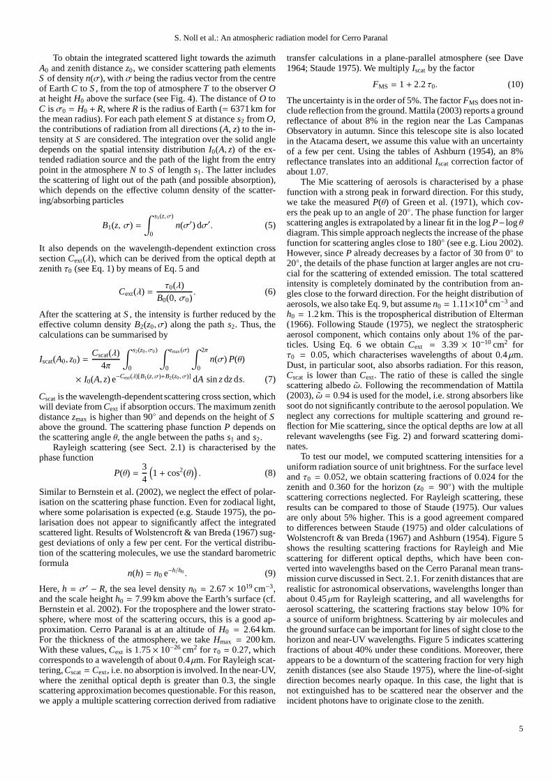
To test our model, we computed scattering intensities for auniform radiation source of unit brightness. For the surface levelandτ0 = 0.052, we obtain scattering fractions of 0.024 for thezenith and 0.360 for the horizon (z0 = 90◦) with the multiplescattering corrections neglected. For Rayleigh scattering, theseresults can be compared to those of Staude (1975). Our valuesare only about 5% higher. This is a good agreement comparedto differences between Staude (1975) and older calculations ofWolstencroft & van Breda (1967) and Ashburn (1954). Figure 5shows the resulting scattering fractions for Rayleigh and Miescattering for different optical depths, which have been con-verted into wavelengths based on the Cerro Paranal mean trans-mission curve discussed in Sect. 2.1. For zenith distances that arerealistic for astronomical observations, wavelengths longer thanabout 0.45µm for Rayleigh scattering, and all wavelengths foraerosol scattering, the scattering fractions stay below 10% fora source of uniform brightness. Scattering by air moleculesandthe ground surface can be important for lines of sight close to thehorizon and near-UV wavelengths. Figure 5 indicates scatteringfractions of about 40% under these conditions. Moreover, thereappears to be a downturn of the scattering fraction for very highzenith distances (see also Staude 1975), where the line-of-sightdirection becomes nearly opaque. In this case, the light that isnot extinguished has to be scattered near the observer and theincident photons have to originate close to the zenith.
5

S. Noll et al.: An atmospheric radiation model for Cerro Paranal
Fig. 5. Intensity of scattered radiation for a uniform source ofunit brightness using the Paranal extinction curve (see Sect. 2.1).Contributions of scattered light into the line of sight are shownfor Rayleigh (solid lines) and Mie scattering (dashed lines) andzenith distances from 0◦ to 80◦ in 10◦ steps plus an extreme valueof 85◦. Except for Rayleigh scattering at very short wavelengths,the scattering intensities increase with zenith distance.
The results of scattering calculations for more realisticsource intensity distributions will be discussed in Sects.3.2, 3.3,and 4.3.
3. Moon, stars, and interplanetary dust
Bright astronomical objects affect night-sky observations by thescattering of their radiation into the line of sight. The relevantinitial radiation sources are the Sun and the summed-up lightof all other stars. The solar radiation must first be scattered byinterplanetary dust grains and the Moon surface to contributeto the night-sky brightness. In the following, we discuss thesescattering-related sky model components, i.e. scattered moon-light (Sect. 3.1), scattered starlight (Sect. 3.2), and zodiacal light(Sect. 3.3). Another source of scattered light is man-made lightpollution, which can be neglected for Cerro Paranal. Patat (2003)did not detect spectroscopic signatures of such contamination.
3.1. Scattered moonlight
For observing dates close to Full Moon, scattered moonlightisby far the brightest component of the optical night-sky back-ground. In particular, blue wavelengths are affected, since theMoon spectrum resembles a solar spectrum and the efficency ofRayleigh/Mie scattering increases towards shorter wavelengths(see Fig. 2).
The Moon can be considered a point source. For this rea-son, it is not necessary to perform the scattering calculationsfor extended sources, as discussed in Sect. 2.2. Instead, a semi-analytical model for the photometricV band by Krisciunas &Schaefer (1991) is used for the sky model, which has been ex-tended into a spectroscopic version.
Based on Krisciunas & Schaefer (1991), we compute theMoon-related sky surface brightness as the sum of the contri-butions from Rayleigh and Mie scattering
Bmoon(λ) = Bmoon,R(λ) + Bmoon,M(λ), (11)
Fig. 6. Effects of atmospheric scattering on radiation originatingoutside of the atmosphere. The displayed radiation sourcesareMoon (blue solid lines), stars (green dashed lines), and interplan-etary dust (red dash-dotted lines). All spectra are normalised tounity at 0.5µm. In theupper panel, a solar spectrum is assumedas top-of-atmosphere spectrum for moonlight (see Sect. 3.1).A slightly reddened solar spectrum is taken for solar radiationscattered at interplanetary dust grains (see Sect. 3.3). Integratedstarlight tends to be redder than sunlight at long wavelengths (seeSect. 3.2). Thelower panel shows the resulting low-resolutionspectra, after light has been scattered in the Earth’s atmosphere,for observing conditions as listed in Table 1. While the lunar andstellar contributions represent scattered radiation only, the dust-related zodiacal light consists of scattered and direct light.
where
Bmoon,R/M(λ) = fR/M(ρ) I∗(λ) t Xmoon(λ) (1− t X0
R/M(λ)). (12)
The empirical scattering functions
fR(ρ) = 105.70(
1.06+ cos2(ρ))
(13)
for Rayleigh scattering and
fM (ρ) = 107.15− (ρ/40) (14)
for Mie scattering depend on the angular separation of Moonand objectρ, which is restricted to angles greater than 10◦. Thefunctions deviate from the ones of Krisciunas & Schaefer (1991)by factors of 2.2 and 10 respectively. These corrections arenec-essary because of the separation of the two scattering processesin Eqs. 11 and 12, the model extension in wavelength, and anoptimisation for the observing conditions at Cerro Paranal. Thetwo correction factors were derived separately from a compari-son with optical VLT data (see Sect. 4.2) by using the increasingimportance of Rayleigh scattering with respect to Mie scatter-ing for shorter wavelengths and larger scattering anglesρ (seeSect. 2.2). The factor of 10 for Mie scattering is highly uncertaindue to a lack of clear constraints from the available data set. TheMoon illuminance is proportional to
I∗ ∝ 10−0.4 (0.026|φ|+4.0×10⁻⁹ φ4) × (dmoon)−2 , (15)
6

S. Noll et al.: An atmospheric radiation model for Cerro Paranal
where the Moon distancedmoon can vary up to 5.5% relative tothe mean value. The lunar phase angleα = 180◦ − φ is the sep-aration angle of Moon and Sun as seen from Earth. It can beestimated from the fractional lunar illumination (FLI) by
α ≈ arccos(1− 2 FLI), (16)
since the influence of the lunar ecliptic latitude onα is negligi-ble. Bmoon also depends on the atmospheric transmission for theairmass of the Moont Xmoon, for which the Patat et al. (2011) ex-tinction curve is used (see Fig. 2). Lastly, it depends on a termthat describes the amount of scattered moonlight in the viewingdirection, which can be roughly approximated by 1− t X0
R/M foreither Rayleigh or Mie scattering and the target airmassX0. Theairmasses of the Krisciunas & Schaefer (1991) model are com-puted using
X =(
1− 0.96 sin2(z))−0.5, (17)
which is especially suited for scattered light, because of alowlimiting airmass at the horizon (cf. Eq. 2).
The Krisciunas & Schaefer model was developed only forthe V band. It can be extended to other wavelength ranges byusing the Cerro Paranal extinction curve (see Sect. 2.1) anditsRayleigh and Mie components for the transmission curvest, tR,and tM in Eq. 12 and by assuming that the Moon spectrum re-sembles the spectrum of the Sun (see Fig. 6). The latter is mod-elled by the solar spectrum of Colina et al. (1996) scaled to theV-band brightness of the moonlight scattering model. For mostsituations, this approach results in systematic uncertainties of nomore than 10% of the total night-sky flux compared to observa-tions. The statistical uncertainties are in the order of 10 to 20%(see Sect. 5). The errors become larger for Full Moon and/ortarget positions close to the Moon (ρ <∼ 30◦). The latter espe-cially concerns red wavelengths, where the contribution ofMieforward scattering to the total intensity of scattered light is par-ticularly high. Consequently, the strongly varying aerosol prop-erties have to be known (which is a challenging task) to allowfor a good agreement of model and observations. However, op-tical astronomical observations close to the Moon are unlikely.Therefore, this is not a critical issue for the sky model.
3.2. Scattered starlight
Like moonlight, starlight is also scattered in the Earth’s atmo-sphere. However, stars are distributed over the entire sky with adistribution maximum towards the centre of the Milky Way. Thisdistribution requires the use of the scattering model for extendedsources described in Sect. 2.2. Since scattered starlight is only aminor component compared to scattered moonlight and zodiacallight (see Fig. 1), it is sufficient for an ETC application to com-pute a mean spectrum. This simplification allows us to avoid theintroduction of sky model parameters such as the galactic coor-dinates, which have a very low impact on the total model flux.
For the integrated starlight (ISL), we use Pioneer 10 data at0.44µm (Toller 1981; Toller et al. 1987; Leinert et al. 1998).These data are almost unaffected by zodiacal light. The small“hole” in the data set towards the Sun has been filled by inter-polation. Since the Pioneer 10 maps do not include stars brighterthan 6.5 mag inV, a global correction given by Melchior et al.(2007) is applied, which increases the total flux by about 16%.Scattering calculations are only performed for the distribution ofstarlight in theB band, i.e. the dependence of this distributionon wavelength is neglected. This approach is supported by cal-culations of Bernstein et al. (2002), indicating that the shapes
of ISL spectra are very stable, except for regions in the dusti-est parts of the Milky Way plane. The wavelength dependenceof the scattered starlight is considered by multiplying therep-resentative ISL mean spectrum of Mattila (1980) by the result-ing wavelength-dependent amount of scattered light (for illustra-tion see Figs. 5 and 6). Since the mean ISL spectrum of Mattilaonly covers wavelengths up to 1µm, we extrapolated the spec-tral range by fitting an average of typical spectral energy distri-butions (SED) for early- and late-type galaxies produced bytheSED-fitting code CIGALE (see Noll et al. 2009). Since the SEDslopes are very similar in the near-IR, the choice of the spectraltype is not crucial. The solar and the mean ISL spectrum are sim-ilar at blue wavelengths, but the ISL spectrum has a redder slopeat longer wavelengths (see Fig. 6). The differences illustrate theimportance of K and M stars for the ISL.
For the desired average scattered light spectrum, we run ourscattering code for different combinations of zenithal opticaldepth, zenith distance, azimuth, and sidereal time for Rayleighand Mie scattering (see Sect. 2.2). The step sizes for the latterthree parameters were 10◦, 45◦, and 2 h, respectively. Zenith dis-tances were only calculated up to 50◦, since this results in a meanairmass of about 1.25 for the covered solid angle, which is typi-cal of astronomical observations. The mean scattering intensitiesfor each optical depthτ0 were then computed. This was trans-lated into a spectrum by using the relation betweenτ0 and wave-length as provided by the Cerro Paranal extinction curve (seeSect. 2.1). Finally, the mean ISL spectrum (normalised to the B-band flux) was multiplied. The sky model code does not changethe final spectrum, except for the molecular absorption, whichis adjusted depending on the bimonthly period (see Sect. 2.1).For the effective absorption airmass, the mean value of 1.25 isassumed.
The resulting spectrum shows an intensity of about13 photons s−1 m−2 µm−1 arcsec−2 at 0.4µm. At 0.6µm, there isonly half of this intensity (see Fig. 6). The results are in goodagreement with the findings of Bernstein et al. (2002).
3.3. Zodiacal light
Zodiacal light is caused by scattered sunlight from interplanetarydust grains in the plane of the ecliptic. A strong contribution isfound for low absolute values of ecliptic latitudeβ and heliocen-tric ecliptic longitudeλ − λ⊙. The brightness distribution pro-vided by Levasseur-Regourd & Dumont (1980) and Leinert etal. (1998) for 0.5µm shows a relatively smooth decrease for in-creasing elongation, i.e. angular separation of object andSun. Astriking exception is the local maximum of the so-called gegen-schein at the antisolar point in the ecliptic. The spectrum of theoptical zodical light is similar to the solar spectrum (Colina etal. 1996), but slightly reddened (see Fig. 6). We apply the rela-tions given in Leinert et al. (1998) to account for the reddening.The correction is larger for smaller elongations. Thermal emis-sion of interplanetary dust grains in the IR is neglected in the skymodel, since the airglow components of atmospheric origin (seeFig. 1) completely outshine it. In the optical, zodiacal light is asignificant component of the sky model. A contribution of about50% is typical of theB andV bands when the Moon is down(see Sect. 5.2). At longer wavelengths, the fraction decreasesdue to the increasing importance of the airglow continuum (seeSect. 4.4).
The model of the zodiacal light presented in Leinert et al.(1998) describes the characteristics of this emission componentoutside of the Earth’s atmosphere. Ground-based observationsof the zodical light also have to take atmospheric extinction into
7
S. Noll et al.: An atmospheric radiation model for Cerro Paranal
account. Since zodiacal light is an extended radiation source, theobserved intensity is a combination of the extinguished top-of-atmosphere emission in the viewing direction and the intensityof light scattered into the line of sight (see Fig. 6). The latter canbe treated by scattering calculations as discussed in Sect.2.2.Scattering out of and into the line of sight leads to an effectiveextinction and this can be expressed by an effective optical depth
τeff = τ0,eff X = fext τ0 X (18)
(cf. Eq. 1; see also Bernstein et al. 2002). Consequently, the scat-tering properties of the zodiacal light can be described by the fac-tor fext alone. This parameter shows only a weak dependence onτ0 and, hence, wavelength. For Rayleigh scattering in the rangefrom U to I band, we find an uncertainty of only about 4%. ForMie scattering fromV to J, a similar variation is found. We ob-tain this result by calculatingfext for a grid of optical depths,zenith distances, azimuths, sideral times, and solar ecliptic lon-gitudes. We take the same grid as for scattered starlight (seeSect. 3.2) plus solar ecliptic longitudes in steps of 90◦, i.e. foreach of the four seasons, one data set was calculated. Scatteringcalculations were only carried out for solar zenith distances ofat least 108◦. This restriction excludes daytime and twilight con-ditions. As for scattered starlight, we consider target zenith dis-tancesz up to 50◦ (see Sect. 3.2). For rare high zodiacal lightintensities, we also let 50◦ < z ≤ 70◦. Thez limits do not signifi-cantly affect fext. A test with 0◦ ≤ z ≤ 70◦ showed a variation offext in the order of a few per cent only.
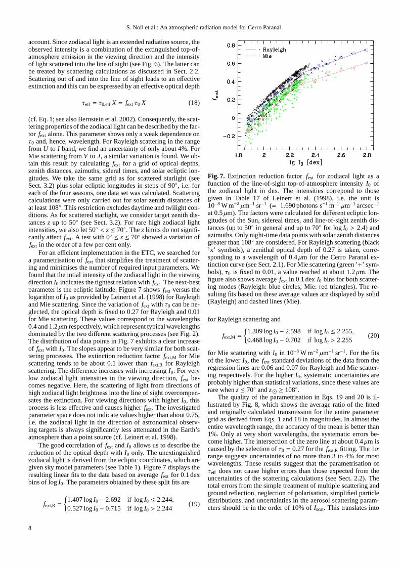
For an efficient implementation in the ETC, we searched fora parametrisation offext that simplifies the treatment of scatter-ing and minimises the number of required input parameters. Wefound that the intial intensity of the zodiacal light in the viewingdirectionI0 indicates the tightest relation withfext. The next-bestparameter is the ecliptic latitude. Figure 7 showsfext versus thelogarithm ofI0 as provided by Leinert et al. (1998) for Rayleighand Mie scattering. Since the variation offext with τ0 can be ne-glected, the optical depth is fixed to 0.27 for Rayleigh and 0.01for Mie scattering. These values correspond to the wavelengths0.4 and 1.2µm respectively, which represent typical wavelengthsdominated by the two different scattering processes (see Fig. 2).The distribution of data points in Fig. 7 exhibits a clear increaseof fext with I0. The slopes appear to be very similar for both scat-tering processes. The extinction reduction factorfext,M for Miescattering tends to be about 0.1 lower thanfext,R for Rayleighscattering. The difference increases with increasingI0. For verylow zodiacal light intensities in the viewing direction,fext be-comes negative. Here, the scattering of light from directions ofhigh zodiacal light brightness into the line of sight overcompen-sates the extinction. For viewing directions with higherI0, thisprocess is less effective and causes higherfext. The investigatedparameter space does not indicate values higher than about 0.75,i.e. the zodiacal light in the direction of astronomical observ-ing targets is always significantly less attenuated in the Earth’satmosphere than a point source (cf. Leinert et al. 1998).
The good correlation offext andI0 allows us to describe thereduction of the optical depth withI0 only. The unextinguishedzodiacal light is derived from the ecliptic coordinates, which aregiven sky model parameters (see Table 1). Figure 7 displays theresulting linear fits to the data based on averagefext for 0.1 dexbins of logI0. The parameters obtained by these split fits are
fext,R =
{
1.407 logI0 − 2.692 if logI0 ≤ 2.244,0.527 logI0 − 0.715 if logI0 > 2.244
(19)
Fig. 7. Extinction reduction factorfext for zodiacal light as afunction of the line-of-sight top-of-atmosphere intensity I0 ofthe zodiacal light in dex. The intensities correpond to thosegiven in Table 17 of Leinert et al. (1998), i.e. the unit is10−8 W m−2 µm−1 sr−1 (= 1.690photons s−1 m−2 µm−1 arcsec−2
at 0.5µm). The factors were calculated for different ecliptic lon-gitudes of the Sun, sidereal times, and line-of-sight zenith dis-tances (up to 50◦ in general and up to 70◦ for log I0 > 2.4) andazimuths. Only night-time data points with solar zenith distancesgreater than 108◦ are considered. For Rayleigh scattering (black’x’ symbols), a zenithal optical depth of 0.27 is taken, corre-sponding to a wavelength of 0.4µm for the Cerro Paranal ex-tinction curve (see Sect. 2.1). For Mie scattering (green ’+’ sym-bols),τ0 is fixed to 0.01, a value reached at about 1.2µm. Thefigure also shows averagefext in 0.1 dexI0 bins for both scatter-ing modes (Rayleigh: blue circles; Mie: red triangles). There-sulting fits based on these average values are displayed by solid(Rayleigh) and dashed lines (Mie).
for Rayleigh scattering and
fext,M =
{
1.309 logI0 − 2.598 if logI0 ≤ 2.255,0.468 logI0 − 0.702 if logI0 > 2.255
(20)
for Mie scattering withI0 in 10−8 W m−2 µm−1 sr−1. For the fitsof the lowerI0, the fext standard deviations of the data from theregression lines are 0.06 and 0.07 for Rayleigh and Mie scatter-ing respectively. For the higherI0, systematic uncertainties areprobably higher than statistical variations, since these values arerare whenz ≤ 70◦ andz⊙ ≥ 108◦.
The quality of the parametrisation in Eqs. 19 and 20 is il-lustrated by Fig. 8, which shows the average ratio of the fittedand originally calculated transmission for the entire parametergrid as derived from Eqs. 1 and 18 in magnitudes. In almost theentire wavelength range, the accuracy of the mean is better than1%. Only at very short wavelengths, the systematic errors be-come higher. The intersection of the zero line at about 0.4µm iscaused by the selection ofτ0 = 0.27 for the fext,R fitting. The 1σrange suggests uncertainties of no more than 3 to 4% for mostwavelengths. These results suggest that the parametrisation ofτeff does not cause higher errors than those expected from theuncertainties of the scattering calculations (see Sect. 2.2). Thetotal errors from the simple treatment of multiple scattering andground reflection, neglection of polarisation, simplified particledistributions, and uncertainties in the aerosol scattering param-eters should be in the order of 10% ofIscat. This translates into
8
S. Noll et al.: An atmospheric radiation model for Cerro Paranal
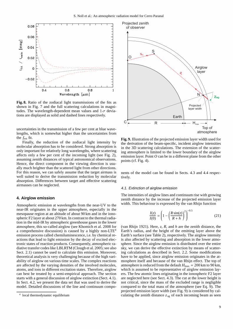
Fig. 8. Ratio of the zodiacal light transmissions of the fits asshown in Fig. 7 and the full scattering calculations in magni-tudes. The wavelength-dependent mean values and 1σ devia-tions are displayed as solid and dashed lines respectively.
uncertainties in the transmission of a few per cent at blue wave-lengths, which is somewhat higher than the uncertainties fromthe fext fit.
Finally, the reduction of the zodiacal light intensity bymolecular absorption has to be considered. Strong absorption isonly important for relatively long wavelengths, where scatteringaffects only a few per cent of the incoming light (see Fig. 2),assuming zenith distances of typical astronomical observations.Hence, the direct component in the viewing direction is usu-ally much brighter than the scattered light from other directions.For this reason, we can safely assume that the target airmassiswell suited to derive the transmission reduction by molecularabsorption. Differences between target and effective scatteringairmasses can be neglected.
4. Airglow emission
Atmospheric emission at wavelengths from the near-UV to thenear-IR originates in the upper atmosphere, especially in themesopause region at an altitude of about 90 km and in the iono-spheric F2 layer at about 270 km. In contrast to the thermal radia-tion in the mid-IR by atmospheric greenhouse gases in the loweratmosphere, this so-called airglow (see Khomich et al. 2008fora comprehensive discussion) is caused by a highly non-LTE4
emission process called chemiluminescence, i.e. by chemical re-actions that lead to light emission by the decay of excited elec-tronic states of reaction products. Consequently, atmospheric ra-diative transfer codes like LBLRTM (Clough et al. 2005; see alsoSect. 2.1) cannot be used to calculate this emission. Moreover,theoretical analysis is very challenging because of the high vari-ability of airglow on various time scales. The complex reactionsare affected by the varying densities of the involved molecules,atoms, and ions in different excitation states. Therefore, airglowcan best be treated by a semi-empirical approach. The sectionstarts with a general discussion of airglow extinction (Sect. 4.1).In Sect. 4.2, we present the data set that was used to derive themodel. Detailed discussions of the line and continuum compo-
4 local thermodynamic equilibrium
Projected zenithof observer
Earth
Top ofatmosphere
R Hmax
Ss2
N
s1
O
C
Airglowlayer
zag
Projectedlayer width
Fig. 9. Illustration of the projected emission layer width used forthe derivation of the beam-specific, incident airglow intensitiesin the 3D scattering calculations. The extension of the scatter-ing atmosphere is limited to the lower boundary of the airglowemission layer. PointO can be in a different plane from the otherpoints (cf. Fig. 4).
nents of the model can be found in Sects. 4.3 and 4.4 respec-tively.
4.1. Extinction of airglow emission
The intensities of airglow lines and continuum rise with growingzenith distance by the increase of the projected emission layerwidth. This behaviour is expressed by the van Rhijn function
I(z)I(0)=
1−
(
R sin(z)R + h
)2
−0.5
(21)
(van Rhijn 1921). Here,z, R, andh are the zenith distance, theEarth’s radius, and the height of the emitting layer above theEarth’s surface (see Table 2), respectively. The airglow intensityis also affected by scattering and absorption in the lower atmo-sphere. Since the airglow emission is distributed over the entiresky, we can derive the effective extinction by means of scatter-ing calculations as described in Sect. 2.2. Some modificationshave to be applied, since airglow emission originates in theat-mosphere itself and because of the van Rhijn effect. The top ofatmosphere is reduced from the defaultHmax = 200 km to 90 km,which is assumed to be representative of airglow emission lay-ers. The few atomic lines originating in the ionospheric F2 layerare neglected here (see Sect. 4.3). The cut at the lower height isnot critical, since the mass of the excluded range is negligiblecompared to the total mass of the atmosphere (see Eq. 9). Theprojected emission layer width (see Fig. 9) is considered bycal-culating the zenith distancez ag of each incoming beam as seen
9
S. Noll et al.: An atmospheric radiation model for Cerro Paranal
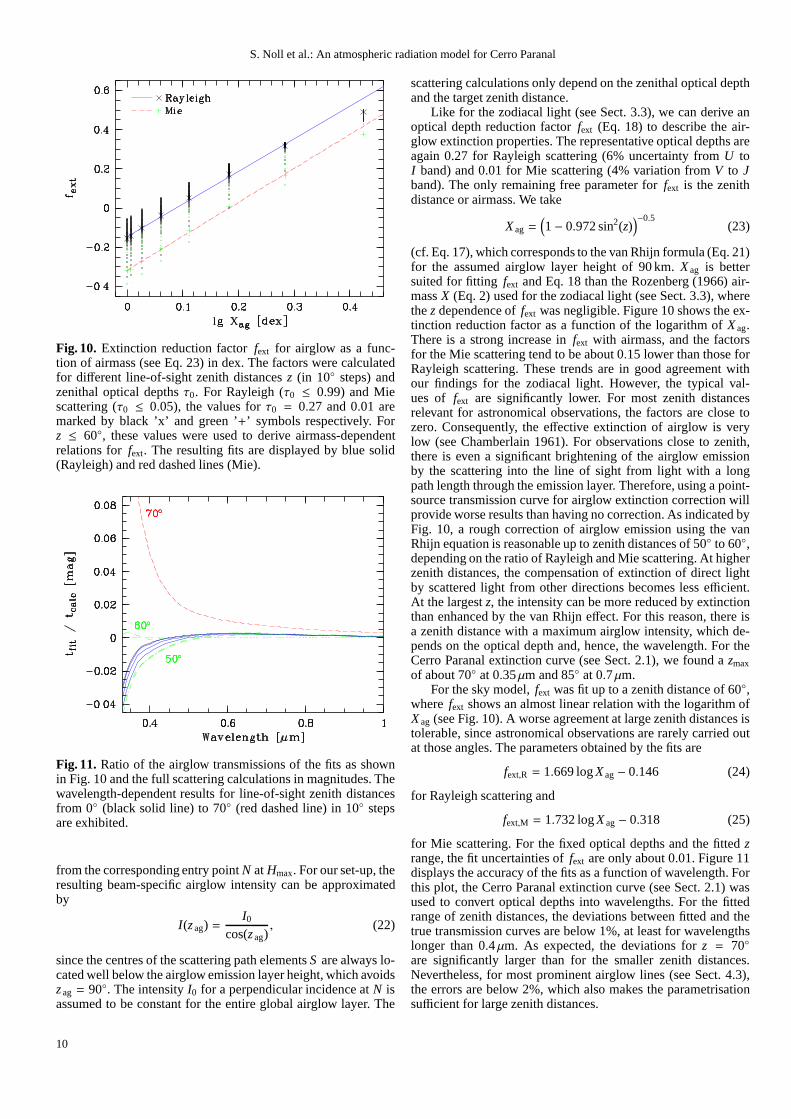
Fig. 10. Extinction reduction factorfext for airglow as a func-tion of airmass (see Eq. 23) in dex. The factors were calculatedfor different line-of-sight zenith distancesz (in 10◦ steps) andzenithal optical depthsτ0. For Rayleigh (τ0 ≤ 0.99) and Miescattering (τ0 ≤ 0.05), the values forτ0 = 0.27 and 0.01 aremarked by black ’x’ and green ’+’ symbols respectively. Forz ≤ 60◦, these values were used to derive airmass-dependentrelations for fext. The resulting fits are displayed by blue solid(Rayleigh) and red dashed lines (Mie).
Fig. 11. Ratio of the airglow transmissions of the fits as shownin Fig. 10 and the full scattering calculations in magnitudes. Thewavelength-dependent results for line-of-sight zenith distancesfrom 0◦ (black solid line) to 70◦ (red dashed line) in 10◦ stepsare exhibited.
from the corresponding entry pointN atHmax. For our set-up, theresulting beam-specific airglow intensity can be approximatedby
I(z ag) =I0
cos(z ag), (22)
since the centres of the scattering path elementsS are always lo-cated well below the airglow emission layer height, which avoidsz ag = 90◦. The intensityI0 for a perpendicular incidence atN isassumed to be constant for the entire global airglow layer. The
scattering calculations only depend on the zenithal optical depthand the target zenith distance.
Like for the zodiacal light (see Sect. 3.3), we can derive anoptical depth reduction factorfext (Eq. 18) to describe the air-glow extinction properties. The representative optical depths areagain 0.27 for Rayleigh scattering (6% uncertainty fromU toI band) and 0.01 for Mie scattering (4% variation fromV to Jband). The only remaining free parameter forfext is the zenithdistance or airmass. We take
X ag =(
1− 0.972 sin2(z))−0.5
(23)
(cf. Eq. 17), which corresponds to the van Rhijn formula (Eq.21)for the assumed airglow layer height of 90 km.X ag is bettersuited for fitting fext and Eq. 18 than the Rozenberg (1966) air-massX (Eq. 2) used for the zodiacal light (see Sect. 3.3), wherethez dependence offext was negligible. Figure 10 shows the ex-tinction reduction factor as a function of the logarithm ofX ag.There is a strong increase infext with airmass, and the factorsfor the Mie scattering tend to be about 0.15 lower than those forRayleigh scattering. These trends are in good agreement withour findings for the zodiacal light. However, the typical val-ues of fext are significantly lower. For most zenith distancesrelevant for astronomical observations, the factors are close tozero. Consequently, the effective extinction of airglow is verylow (see Chamberlain 1961). For observations close to zenith,there is even a significant brightening of the airglow emissionby the scattering into the line of sight from light with a longpath length through the emission layer. Therefore, using a point-source transmission curve for airglow extinction correction willprovide worse results than having no correction. As indicated byFig. 10, a rough correction of airglow emission using the vanRhijn equation is reasonable up to zenith distances of 50◦ to 60◦,depending on the ratio of Rayleigh and Mie scattering. At higherzenith distances, the compensation of extinction of directlightby scattered light from other directions becomes less efficient.At the largestz, the intensity can be more reduced by extinctionthan enhanced by the van Rhijn effect. For this reason, there isa zenith distance with a maximum airglow intensity, which de-pends on the optical depth and, hence, the wavelength. For theCerro Paranal extinction curve (see Sect. 2.1), we found azmaxof about 70◦ at 0.35µm and 85◦ at 0.7µm.
For the sky model,fext was fit up to a zenith distance of 60◦,where fext shows an almost linear relation with the logarithm ofX ag (see Fig. 10). A worse agreement at large zenith distances istolerable, since astronomical observations are rarely carried outat those angles. The parameters obtained by the fits are
fext,R = 1.669 logX ag− 0.146 (24)
for Rayleigh scattering and
fext,M = 1.732 logX ag− 0.318 (25)
for Mie scattering. For the fixed optical depths and the fittedzrange, the fit uncertainties offext are only about 0.01. Figure 11displays the accuracy of the fits as a function of wavelength.Forthis plot, the Cerro Paranal extinction curve (see Sect. 2.1) wasused to convert optical depths into wavelengths. For the fittedrange of zenith distances, the deviations between fitted andthetrue transmission curves are below 1%, at least for wavelengthslonger than 0.4µm. As expected, the deviations forz = 70◦
are significantly larger than for the smaller zenith distances.Nevertheless, for most prominent airglow lines (see Sect. 4.3),the errors are below 2%, which also makes the parametrisationsufficient for large zenith distances.
10
S. Noll et al.: An atmospheric radiation model for Cerro Paranal
Apart from scattering, molecular absorption in the lower at-mosphere affects the observed airglow intensity. However, inthe optical these absorptions are usually small (see Fig. 2).Exceptions are the airglow O2(b-X)(0-0) and O2(b-X)(1-0)bands at 762 and 688 nm, which suffer from heavy self-absorption at low altitudes, and can be observed as absorptionbands only. As discussed in Sect. 3.3, the effective molecularabsorption can be well approximated by taking the transmissionspectrum for the target zenith distance. For the airglow contin-uum component, this is easily applied. For the line component,this is challenging, since airglow emission as well as telluric ab-sorption lines are very narrow. Therefore, an effective absorptionfor each airglow line has to be derived at very high resolution.Resolving the airglow lines requires resolutions in the order of106. The absorption lines tend to be broader than the emissionlines. LBLRTM (see Clough et al. 2005) easily produces spec-tra with the required resolution. For the airglow emission,weuse a line list with good wavelength accuracy, as discussed inSect. 4.3. In the upper atmosphere, broadening of lines by colli-sions can be neglected due to the low density (see Khomich et al.2008). Thus, the shape and width of airglow lines are determinedby Doppler broadening, which can be derived by the molecularweight of the species and ambient temperature. The latter isinthe order of 200 K in the mesopause region, which explains thelow Doppler widths. For example, the FWHM of an OH line(see Sect. 4.3) at 0.8µm is about 2 picometers (pm). The fewlines originating in the thermospheric ionosphere experience dis-tinctly higher temperatures of about 1000 K. The line absorptioncorrection is applied as the multiplication of the initial line in-tensities by the suitable line transmissions from a pre-calculatedlist, which is derived from the library transmission spectrum cor-responding to the selected observing conditions (see Sect.2.1).
The airglow line absorptions show significant deviationsfrom the continuum absorption at similar wavelengths. As al-ready mentioned, strong self-absorption is found for the O2ground state transitions in the optical. However, most other air-glow lines tend to be less absorbed than the continuum. In partic-ular, the H2O absorption bands (see Sect. 2.1) have little effect.This can be explained by the relatively low width of the telluriclines compared to the typical distance between strong absorptionlines. Hence, the chance to find an airglow line at the centre of astrong absorption feature is relatively low.
4.2. Data set for airglow analysis
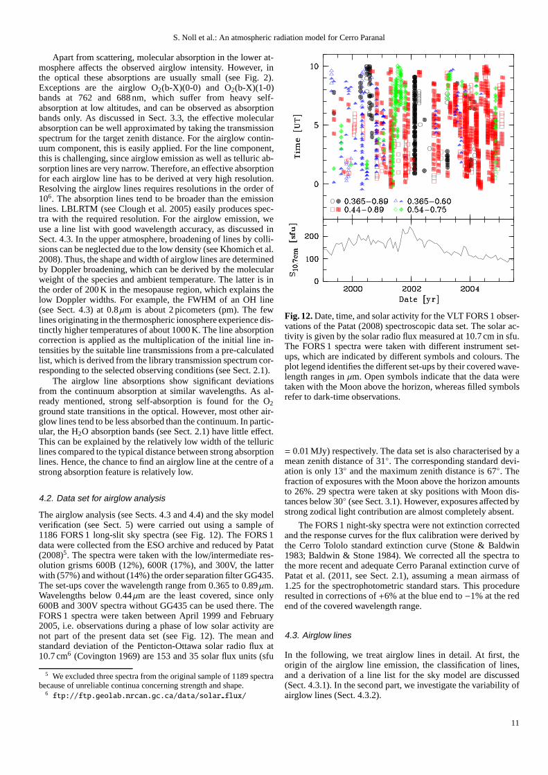
The airglow analysis (see Sects. 4.3 and 4.4) and the sky modelverification (see Sect. 5) were carried out using a sample of1186 FORS 1 long-slit sky spectra (see Fig. 12). The FORS 1data were collected from the ESO archive and reduced by Patat(2008)5. The spectra were taken with the low/intermediate res-olution grisms 600B (12%), 600R (17%), and 300V, the latterwith (57%) and without (14%) the order separation filter GG435.The set-ups cover the wavelength range from 0.365 to 0.89µm.Wavelengths below 0.44µm are the least covered, since only600B and 300V spectra without GG435 can be used there. TheFORS 1 spectra were taken between April 1999 and February2005, i.e. observations during a phase of low solar activityarenot part of the present data set (see Fig. 12). The mean andstandard deviation of the Penticton-Ottawa solar radio fluxat10.7 cm6 (Covington 1969) are 153 and 35 solar flux units (sfu
5 We excluded three spectra from the original sample of 1189 spectrabecause of unreliable continua concerning strength and shape.
6 ftp://ftp.geolab.nrcan.gc.ca/data/solar flux/
Fig. 12. Date, time, and solar activity for the VLT FORS 1 obser-vations of the Patat (2008) spectroscopic data set. The solar ac-tivity is given by the solar radio flux measured at 10.7 cm in sfu.The FORS 1 spectra were taken with different instrument set-ups, which are indicated by different symbols and colours. Theplot legend identifies the different set-ups by their covered wave-length ranges inµm. Open symbols indicate that the data weretaken with the Moon above the horizon, whereas filled symbolsrefer to dark-time observations.
= 0.01 MJy) respectively. The data set is also characterised by amean zenith distance of 31◦. The corresponding standard devi-ation is only 13◦ and the maximum zenith distance is 67◦. Thefraction of exposures with the Moon above the horizon amountsto 26%. 29 spectra were taken at sky positions with Moon dis-tances below 30◦ (see Sect. 3.1). However, exposures affected bystrong zodical light contribution are almost completely absent.
The FORS 1 night-sky spectra were not extinction correctedand the response curves for the flux calibration were derivedbythe Cerro Tololo standard extinction curve (Stone & Baldwin1983; Baldwin & Stone 1984). We corrected all the spectra tothe more recent and adequate Cerro Paranal extinction curveofPatat et al. (2011, see Sect. 2.1), assuming a mean airmass of1.25 for the spectrophotometric standard stars. This procedureresulted in corrections of+6% at the blue end to−1% at the redend of the covered wavelength range.
4.3. Airglow lines
In the following, we treat airglow lines in detail. At first, theorigin of the airglow line emission, the classification of lines,and a derivation of a line list for the sky model are discussed(Sect. 4.3.1). In the second part, we investigate the variability ofairglow lines (Sect. 4.3.2).
11

S. Noll et al.: An atmospheric radiation model for Cerro Paranal
Table 2. Basic properties of the Paranal airglow line and continuum (0.543µm) variability as derived from the Patat (2008) spectraldata set.
Property Unit [O I] 5577 Na I D [O I] 6300,6364 OH(7,0)-(6,2) O2(b-X)(0-1) 0.543µm
h layer km 97 92 270 87 94 90Nspec – 1186 1046 1046 1046 839 874〈I〉a phot s−1 m−2 arcsec−2 3.6 0.81 3.5 60. 6.0 80.b
(1.6) (0.48) (3.4) (19.) (2.5) (31.b )Rc 190. 43. 190. 3200. 320. 4.3d
(90.) (26.) (180.) (1000.) (130.) (1.6d )msun
e sfu−1 0.0087 0.0011 0.0068 0.0001 0.0063 0.0061Pseason,min
f – 1 1 1 5 5 1fseason,min – 0.86 0.54 0.30 0.82 0.71 0.81
Pseason,maxf – 3 3 3 6 3 3
fseason,max – 1.44 1.84 1.51 1.14 1.33 1.24
Notes.(a) Mean intensity and variability (in parentheses) for solar cycles 19 to 23.(b) In photons s−1 m−2 µm−1 arcsec−2.(c) 1 R (Rayleigh)≈ 0.018704 phot s−1 m−2 arcsec−2.(d) In R nm−1.(e) Slope for solar activity correction relative to mean solar radio flux for cycles 19 to 23 (≈ 129 sfu).( f ) Two-month bin with minimum or maximum correction factor: 1= Dec/Jan, 2= Feb/Mar, 3= Apr/May, 4= Jun/Jul, 5= Aug/Sep, 6= Oct/Nov.
0.4 0.5 0.6 0.7 0.8Wavelength [µm]
0
2000
4000 Class 5: O2
0
2000
4000 Class 4: OH
0
2000
4000
Rad
ianc
e
0
2000
4000 Class 1: green OI
0
2000
4000 Class 2: NaID
x 30
Class 3: red OI
x 30
x 10
x 30
Fig. 13. Variability classes for airglow emission lines. The fol-lowing groups are defined: (1) green O I, (2) Na I D, (3) red O I,(4) OH, and (5) O2. The weak lines (green curves) are scaled bya factor of 30 for Na I D, red O I, and O2, and a factor of 10 forOH.
4.3.1. Line classes and line list
The most prominent optical airglow line is [O I] 5577 (seeFig. 13, panel 1). Its dominant component at an altitude of about97 km is probably produced by the process described in Barth &Hildebrand (1961). The crucial reactions are
O+O+M → O∗2 +M, (26)
O∗2 +O→ O2 +O(1S), (27)
andO(1S)→ O(1D) + 557.7 nm, (28)
where M is an arbitrary reaction partner. The first reaction(Eq. 26) also plays an important role for the emission bands ofmolecular oxygen. In order to start the three body collision, oxy-gen molecules have to be split by hard UV photons:
O2 + hν→ O+O. (29)
This process mainly occurs during the day by solar UV radia-tion, which implies that the oxygen airglow intensity dependson the solar activity and observing time. The O(1D) state canlead to [O I] 6300 emission (see Fig. 13, panel 3). However, inthe mesopause the deactivation of this metastable state is mostlycaused by collisions. Hence, strong [O I] 6300 emission is re-stricted to the thermosphere at altitudes of about 270 km. Incon-trast to the mesosphere, the excitation there is caused by disso-ciative recombination (Bates 1982), i.e. it depends on the elec-tron density:
O+2 + e− → O+O(1D). (30)
The ionised molecular oxygen is produced by the charge transferreaction
O+ +O2→ O+2 +O. (31)
The amount of ionised oxygen and free electrons depends onthe solar radiation. The most striking features of the airglow arethe Meinel OH bands (Meinel et al. 1954), which dominate atred optical wavelengths and beyond (see Fig. 13, panel 4). The
12

S. Noll et al.: An atmospheric radiation model for Cerro Paranal
fundamental and overtone rotational-vibrational transitions aremainly produced by the Bates-Nicolet (1950) mechanism
O3 + H→ OH∗ +O2. (32)
Most emission originates in a relatively thin layer at 87 km.Finally, the upper state of the prominent D lines of neutralsodium at 589.0 and 589.6nm (see Fig. 13, panel 2), which orig-inate in a thin layer at 92 km, is probably excited by
NaO+O→ Na(2P)+O2 (33)
(Chapman 1939). NaO appears to be provided by
Na+O3→ NaO+O2. (34)
For studying airglow intensity and variability, we assignedthe optical airglow lines to five classes, for which a similiar vari-ability is reasonable or could be proved by a correlation analy-sis (see Patat 2008). These classes are (1) green O I, (2) Na I D,(3) red O I, (4) OH, and (5) O2 (see Fig. 13). The first threeclasses correspond to atomic lines, the other two groups com-prise molecular bands. The O I lines are divided into two classes.The green O I line at 557.7 nm mainly originates at altitudesslightly below 100 km, while the other significant O I lines (allbeing in the red wavelength range) tend to originate at altitudesgreater than 200 km (see Khomich et al. 2008). Moreover, thekind of chemical reactions are also different, since the high al-titude emissions are usually related to reactions involving ions(see above). Another small group consists of the sodium Dlines and a weak K I line at 769.9nm (see Fig. 13, panel 2).By far most of the airglow lines belong to the two classes ofmolecules which produce band structures by ro-vibrationaltran-sitions. The OH electronic ground state (X-X) bands with up-per vibrational levelsv′ ≤ 9 cover the wavelength range long-wards of about 0.5µm with increasing band strength towardslonger wavelengths. There are several electronic transitions withband systems for O2 in the optical. Relatively weak bands ofthe Herzberg I (A-X) and Chamberlain (A’-a) systems originateat near-UV and blue wavelengths (see Cosby et al. 2006). Atwavelengths longwards of 0.6µm, the atmospheric (b-X) bandsystem produces several strong bands. However, those bandsrelated to the vibrationalv = 0 level at the electronic groundstate X are strongly absorbed in the lower atmosphere (seeSect. 4.1). Therefore, the only remaining strong band in thein-vestigated wavelength range is O2(b-X)(0-1) at about 864.5nm(see Fig. 13, panel 5). Variability studies of O2 have to rely onthe results from this band.
For the identification of airglow lines and as an input line listfor the sky model, we use the list of Cosby et al. (2006). It con-sists of 2805 entries with information on the line wavelengths,widths, fluxes, and line identities. It is based on the sky emis-sion line atlas of Hanuschik (2003), which was obtained fromatotal of 44 high-resolution (R ∼ 45000) VLT UVES spectra. Bycombining different instrumental set-ups, the wavelength rangefrom 0.314 to 1.043µm could be covered. The accuracy of thewavelength calibration is better than 1 pm (cf. Sect. 4.1). TheUVES spectra were flux calibrated by means of the Tug (1977)extinction curve. Since the use of a point-source extinction curvefor the airglow leads to systematic errors (see Sect. 4.1) and theLa Silla extinction curve was used for Cerro Paranal, we cor-rected the line extinction by means of the Patat et al. (2011)ex-tinction curve and the recipes given in Eqs. 24 and 25. At thelower wavelength limit, this caused an extreme correction factorof 0.37 and in the range of the O2(b-X)(0-0) band a maximumfactor of 4.5 due to the line molecular absorption correction (see
Sect. 4.1). However, for the strongest 100 lines up to a wave-length of 0.92µm, we only obtain a mean correction factor of0.98. In a similar way as discussed in Sect. 4.2 for the Patat(2008) data, we considered how a different extinction curve af-fects the response curves for flux calibration. Here, we obtain forthe 100 brightest lines another correction of 0.97, which isrep-resentative of the factors for the entire wavelength range,whichrange from 0.95 to 1.00. Due to a gap at about 0.86µm, theCosby et al. (2006) line list misses a part of the important O2(b-X)(0-1) band. There is an unpublished UVES 800U spectrumrelated to the study of Hanuschik (2003) that covers the gap.Weused this spectrum to measure the line intensities. Determined bya few overlapping lines, the resulting intensities were then scaledto those in the line list. For the line identification, we consideredO2 and OH line data from the HITRAN database (see Rothmanet al. 2009). For the final line list for the sky model, the inten-sities of each variability class were scaled to match the meanvalue derived from the variability analysis (see below). Finally,the line wavelengths were converted from air to vacuum by
λvac = n λair. (35)
The refractive index
n = 1+ 10−8
(
8342.13+2406030130− σ2
+15997
38.9− σ2
)
, (36)
whereσ = λ−1 andλ is in µm (Edlen 1966). This formula isalso used internally in the sky model code if an output in airwavelengths is required (see Table 1).
4.3.2. Line variability
In general, airglow lines show strong variability on time scalesranging from minutes to years. This behaviour can be explainedby the solar activity cycle, seasonal changes in the temperature,pressure, and chemical composition of the emission layers,theday-night contrast, dynamical effects such as internal gravitywaves and geomagnetic disturbances (see Khomich et al. 2008).In order to consider airglow variability in our sky model, wede-rived a semi-empirical model based on 1186 VLT FORS 1 skyspectra (Patat 2008; see Sect. 4.2). The demands on an airglowvariability model are twofold. First of all, it should include allmajor predictable variability properties. This excludes stochas-tic wave phenomena like gravity waves. Second, the derivedparametrisation should be robust. For studying many variabilitytriggers, about 1000 spectra is not statistically a high number.For this reason, only a few variables can be analysed. Since thisneglection leads to higher uncertainties, an ideal set of param-eters has to be found that provides statistically significant, pre-dictable variations. For our airglow model, we studied the effectof solar activity, period of the year, and time of the night. Theanalysis was carried out for each of the five variability classes(see Fig. 13).
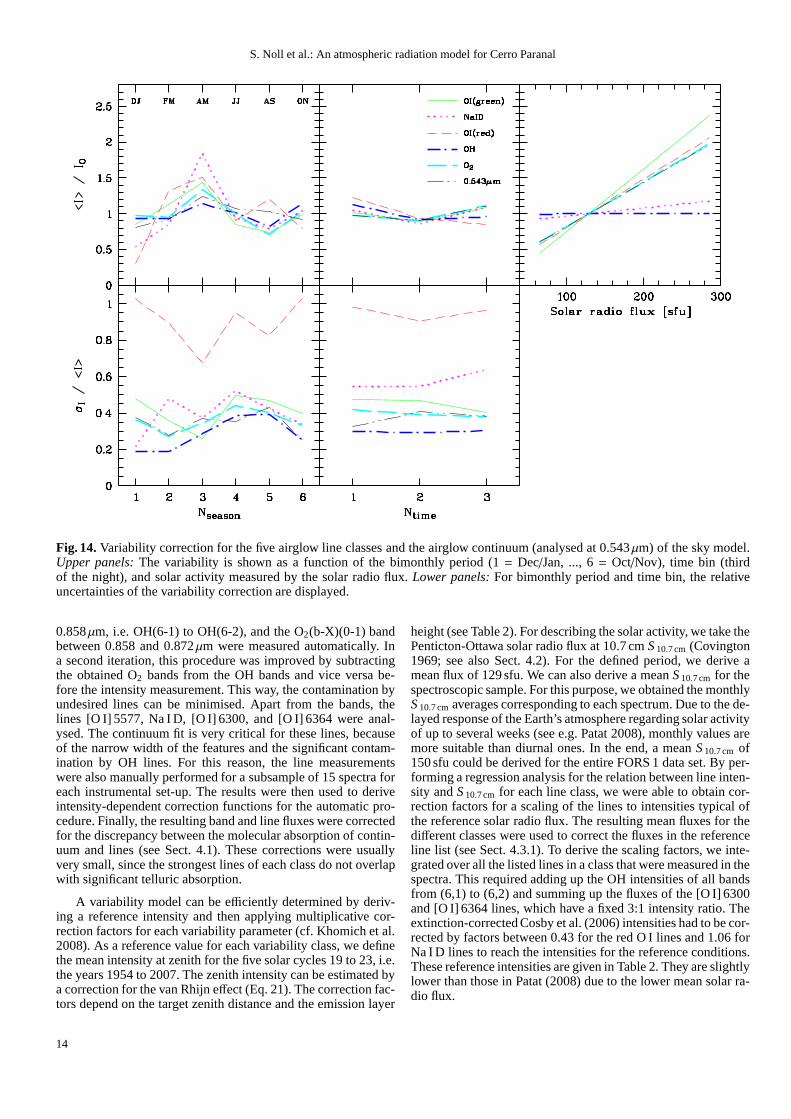
The first step for measuring the line and band fluxes wasthe subtraction of scattered moonlight, scattered starlight, andzodiacal light by using the recipes given in Sect. 3. The result-ing spectra were then corrected for airglow continuum extinc-tion as described in Sect. 4.1. For the flux measurements, con-tinuum windows were defined. Their central wavelengths arelisted in Table 3. The widths were 4 nm, except for 0.767µm,where 0.3 nm was chosen to reduce the contamination by strongOH lines and the O2(b-X)(0-0) band (see also Sects. 4.1 and4.4). Then, the continuum fluxes were interpolated to obtainlineand band intensities. The hydroxyl bands between 0.642 and
13
S. Noll et al.: An atmospheric radiation model for Cerro Paranal
Fig. 14. Variability correction for the five airglow line classes andthe airglow continuum (analysed at 0.543µm) of the sky model.Upper panels: The variability is shown as a function of the bimonthly period (1 = Dec/Jan, ..., 6= Oct/Nov), time bin (thirdof the night), and solar activity measured by the solar radioflux. Lower panels: For bimonthly period and time bin, the relativeuncertainties of the variability correction are displayed.
0.858µm, i.e. OH(6-1) to OH(6-2), and the O2(b-X)(0-1) bandbetween 0.858 and 0.872µm were measured automatically. Ina second iteration, this procedure was improved by subtractingthe obtained O2 bands from the OH bands and vice versa be-fore the intensity measurement. This way, the contamination byundesired lines can be minimised. Apart from the bands, thelines [O I] 5577, Na I D, [O I] 6300, and [O I] 6364 were anal-ysed. The continuum fit is very critical for these lines, becauseof the narrow width of the features and the significant contam-ination by OH lines. For this reason, the line measurementswere also manually performed for a subsample of 15 spectra foreach instrumental set-up. The results were then used to deriveintensity-dependent correction functions for the automatic pro-cedure. Finally, the resulting band and line fluxes were correctedfor the discrepancy between the molecular absorption of contin-uum and lines (see Sect. 4.1). These corrections were usuallyvery small, since the strongest lines of each class do not overlapwith significant telluric absorption.
A variability model can be efficiently determined by deriv-ing a reference intensity and then applying multiplicativecor-rection factors for each variability parameter (cf. Khomich et al.2008). As a reference value for each variability class, we definethe mean intensity at zenith for the five solar cycles 19 to 23,i.e.the years 1954 to 2007. The zenith intensity can be estimatedbya correction for the van Rhijn effect (Eq. 21). The correction fac-tors depend on the target zenith distance and the emission layer
height (see Table 2). For describing the solar activity, we take thePenticton-Ottawa solar radio flux at 10.7 cmS 10.7 cm (Covington1969; see also Sect. 4.2). For the defined period, we derive amean flux of 129 sfu. We can also derive a meanS 10.7 cm for thespectroscopic sample. For this purpose, we obtained the monthlyS 10.7 cm averages corresponding to each spectrum. Due to the de-layed response of the Earth’s atmosphere regarding solar activityof up to several weeks (see e.g. Patat 2008), monthly values aremore suitable than diurnal ones. In the end, a meanS 10.7 cm of150 sfu could be derived for the entire FORS 1 data set. By per-forming a regression analysis for the relation between lineinten-sity andS 10.7 cm for each line class, we were able to obtain cor-rection factors for a scaling of the lines to intensities typical ofthe reference solar radio flux. The resulting mean fluxes for thedifferent classes were used to correct the fluxes in the referenceline list (see Sect. 4.3.1). To derive the scaling factors, we inte-grated over all the listed lines in a class that were measuredin thespectra. This required adding up the OH intensities of all bandsfrom (6,1) to (6,2) and summing up the fluxes of the [O I] 6300and [O I] 6364 lines, which have a fixed 3:1 intensity ratio. Theextinction-corrected Cosby et al. (2006) intensities had to be cor-rected by factors between 0.43 for the red O I lines and 1.06 forNa I D lines to reach the intensities for the reference conditions.These reference intensities are given in Table 2. They are slightlylower than those in Patat (2008) due to the lower mean solar ra-dio flux.
14

S. Noll et al.: An atmospheric radiation model for Cerro Paranal
Fig. 15. Variability correction factors and their errors dependingon bimonthly period (1= Dec/Jan, ..., 6= Oct/Nov) and night time(third of the night: evening, midnight, morning) for the fiveairglow line classes and the airglow continuum (analysed at0.543µm)of the sky model. Data points only differing in the bimonthly period are connected by lines.
The S 10.7 cm-dependent linear fits to the airglow intensities(see also Patat 2008) are also used to parametrise a correctionof solar activity for our sky model. Even though the parametri-sation is reasonable (cf. Khomich et al. 2008), there may besystematic deviations for monthlyS 10.7 cm beyond the data setlimits of 95 and 228 sfu (see Sect. 4.2). With the dependenceon solar radio flux removed, seasonal and nocturnal variationscan be investigated. Since the intensity has a complex depen-dence on these parameters (see Khomich et al. 2008), we di-vided the data set into 6 seasonal and 3 night-time bins. In thesame way as described in Sect. 2.1 for the transmission curves,the two-month periods start with the December/January combi-nation. The night, as limited by the astronomical twilight,is al-ways divided into three periods of equal length. This means thatin winter the periods are longer than in summer. For the latitudeof Cerro Paranal (see Sect. 1), the Dec/Jan night bins are about30% shorter than the Jun/Jul bins. Due to the additional con-sideration of specific averages over the entire year and/or night,the total number of bins defined for the sky model is 28 (seealso Table 1). Since the number of spectra in the individual binsdiffered by an order of magnitude, the average values over sev-eral bins could be biased. Therefore, all bins were filled withthe same number of spectra by randomly adding spectra fromthe same bin, i.e. the data were cloned. This approach was alsoused for deriving the reference intensities. As a consequence,the mean solar radio flux of the data set changed from 153 (seeSect. 4.2) to 150 sfu. Finally, mean values and standard devia-
tions were calculated for the individual and multiple bins usingthe original and bias-corrected data sets respectively. While themean value provides an intensity correction factor for seasonaland/or night-time dependence, the standard deviation indicatesthe contribution of neglected variability components to the mea-sured intensity. It also depends on the data quality, uncertaintiesin the analysis, and the accuracy of other sky model components.Therefore, the standard deviation of each bin should be an upperlimit for the unmodelled airglow variability in the investigateddata set.
The results of the airglow variability study are summarisedin Table 2, and Figs. 14 and 15. The solar activity strongly influ-ences the intensities of O I and O2, where the slopes are 0.0063to 0.0087sfu−1. On the other hand, weak or no significant corre-lations are present for sodium and hydroxyl. These findings arein qualitative agreement with the relations given in Khomich etal. (2008), who provide 0.0025 to 0.0060sfu−1 for the first andabout 0.0015sfu−1 for the second group from measurements atdifferent observing sites (mainly in the Northern Hemisphere).The relatively low value of 0.0025sfu−1 for the green O I linecompared to 0.0087sfu−1 from our model is not critical. A moreprecise latitude-dependent analysis of satellite-based data by Liu& Shepherd (2008) resulted in 0.0065sfu−1 for the latitude rangefrom−20◦ to −30◦. For−30◦ to −40◦ they even obtain the sameslope as in our model. The discrepancies in the results from lit-erature show that quantitative comparisons are difficult with dif-ferent observing sites, observing periods, instruments, and anal-
15

S. Noll et al.: An atmospheric radiation model for Cerro Paranal
ysis methods. Solar activity directly affects the Earth’s atmo-sphere by the amount of hard UV photons. The higher the pho-ton energy, the more the production rate depends on solar ac-tivity (see Nicolet 1989). This relation appears to be importantfor O I and O2 airglow emission, which depends on the dissocia-tion or ionisation of molecular oxygen by hard UV photons (seeSect. 4.3.1).
Significant dependence on the bimonthly period is found forall line classes (see Fig. 14). Na I D and the red O I lines indi-cate the strongest variability with a maximum intensity ratio of3.4 and 5.0 respectively, whereas OH shows the weakest depen-dence with a ratio of 1.4 (see Table 2). Except for OH, the max-imum is reached in the autumn months April and May. For theatomic lines, the minimum arises in Dec/Jan, and for the molec-ular bands, it appears to be in Aug/Sep. The variations found re-flect the semi-annual oscilliations of airglow intensity (cf. Patat2008), which are characterised by two maxima and minima ofdifferent strength per year. Complex empirical relations basedon long-term observations at many observing sites as given byKhomich et al. (2008) can be used to estimate this intensity vari-ation. However, since these relations depend on rough interpola-tions and extrapolations, they can only provide a coarse variabil-ity pattern for an arbitrary location on Earth. Nevertheless, theserelations confirm the amplitude of the variations and the roughpositions of the maxima and minima. For example, the peak-to-peak ratios for green O I, Na I D, and OH are 1.4, 3.8, and 1.3,which agrees well with the sky model values 1.7, 3.4, and 1.4(see Table 2). Apart from the obvious change of the incident so-lar radiation, the seasonal variations are related to changes inthe layer heights of the atmospheric constituents, changesin thetemperature profiles, and the dynamics of the upper atmospherein general.
Averaged over the year, the dynamical range of the night-time variations is in the order of 20 to 30%, which is distinctlysmaller than the seasonal variations. Only the red O I lines showa clear decrease by a factor of 1.4 from the beginning to theend of the night. Usually, the diurnal variations are the largest inairglow intensity with possible amplitudes of several orders ofmagnitude (see Khomich et al. 2008). Since we exclude daytimeand twilight conditions with direct solar radiation, the variabil-ity is much smaller. In addition, the use of only three bins cansmooth out the intensity variations. However, an investigationwith the unbinned data (see also Patat 2008) and results fromphotometric studies (Mattila et al. 1996; Benn & Ellison 1998;Patat 2003) confirm the absence of strong trends. Averaging overall bimonthly periods appears to cancel part of the variability.This is illustrated in Fig. 15, which shows the bimonthly de-pendence of the airglow intensity for each third of the night.At midnight, i.e. the maximum time distance to the twilight,the intensities of the mesopause lines tend to reach a minimum.However, the deviations from the intensities of the eveningandmorning bins appear to be a function of season. While in winterthe differences reach a maximum, summer has the smallest dif-ferences. This behaviour can be explained by the night lengthsat Cerro Paranal, which can vary by more than 30%. In sum-mer, the average length of time from the closest twilight is sig-nificantly smaller than in winter. This dependence supportsthecommon treatment of seasonal and night-time variations in thesky model.
The residual statistical variations of the airglow model, asdepicted in Fig. 14, are mainly between 20 and 50% for the linesoriginating in the mesopause region. The smallest uncertaintiesare found for OH in summer, whereas the ionospheric O I linesindicate very strong unpredictable variations with an amplitude
Table 3. Airglow/residual continuum and its intensity variationrelative to the reference wavelength 0.543µm.
λ [µm] 〈I〉/I0 σI/I0 σI/〈I〉
0.369 0.92 0.13 0.140.387 0.65 0.11 0.170.420 0.69 0.10 0.150.450 0.70 0.11 0.150.480 0.79 0.11 0.140.510 0.79 0.09 0.120.543 1.00 0.00 0.000.575 1.41 0.25 0.180.608 1.40 0.29 0.200.642 1.18 0.19 0.160.675 1.14 0.13 0.120.720 1.32 0.21 0.160.767 1.64 0.46 0.280.820 2.57 0.67 0.260.858 3.56 1.06 0.300.872 3.76 1.12 0.30
Notes. The reference continuum intensity at 0.543µm is79.8 photons s−1 m−2 µm−1 arcsec−2 or 4.27 R nm−1.
comparable to the intensity itself (see also Patat 2008). This be-haviour is caused by the aurora-like intensity fluctuationsfromgeomagnetic disturbances. This effect is particularly importantfor Cerro Paranal, because of its location close to one of thetwoactive regions about 20◦ on either side of the geomagnetic equa-tor (Roach & Gordon 1973).
4.4. Airglow continuum
The airglow continuum is the least understood emission compo-nent of the night sky. In the optical, the best-documented processis a chemiluminescent reaction of nitric oxide and atomic oxy-gen in the mesopause region as proposed by Krassovsky (1951):
NO+O→ NO2 + hν (37)
NO2 +O→ NO+O2. (38)
This reaction appears to dominate the visual and is expectedtohave a broad maximum at about 0.6µm (see Sternberg & Ingham1972; von Savigny et al. 1999; Khomich et al. 2008). Reactionsof NO and ozone could be important for the airglow continuumat red to near-IR wavelengths (Clough & Thrush 1967; Kenner& Ogryzlo 1984). In particular, the reaction
NO+O∗3→ NO∗2 +O2 (39)
is expected to significantly contribute to the optical by contin-uum emission with a broad maximum at about 0.85µm (Kenner& Ogryzlo 1984; Khomich et al. 2008). Finally, a pseudo con-tinuum by molecular band emission produced by
Fe+O3→ FeO∗ +O2 (40)
(West & Broida 1975) could be an important component of thecontinuum between 0.55 and 0.65µm (Jenniskens et al. 2000;Evans et al. 2010; Saran et al. 2011).
The airglow continuum was analysed in a similar way as theairglow emission lines. As reported in Sect. 4.3.2, the deriva-tion of line intensities already required the measurement of air-glow continuum fluxes in suitable windows (see Table 3). These
16
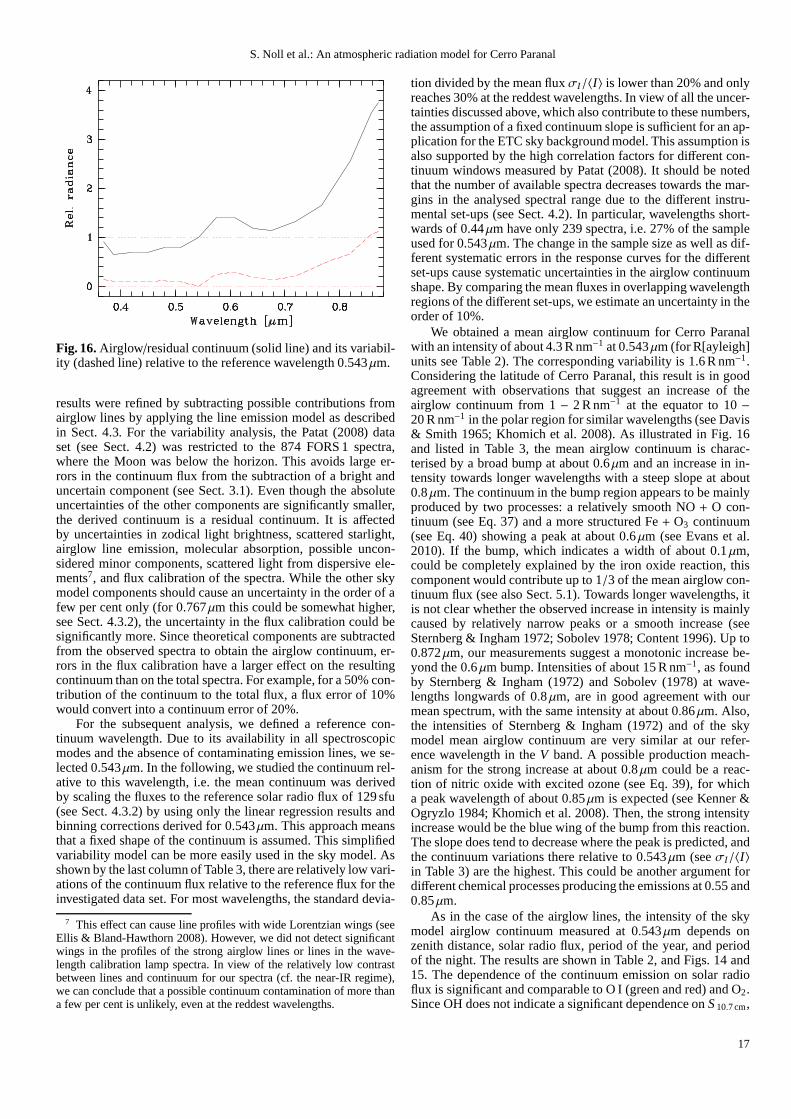
S. Noll et al.: An atmospheric radiation model for Cerro Paranal
Fig. 16. Airglow/residual continuum (solid line) and its variabil-ity (dashed line) relative to the reference wavelength 0.543µm.
results were refined by subtracting possible contributionsfromairglow lines by applying the line emission model as describedin Sect. 4.3. For the variability analysis, the Patat (2008)dataset (see Sect. 4.2) was restricted to the 874 FORS 1 spectra,where the Moon was below the horizon. This avoids large er-rors in the continuum flux from the subtraction of a bright anduncertain component (see Sect. 3.1). Even though the absoluteuncertainties of the other components are significantly smaller,the derived continuum is a residual continuum. It is affectedby uncertainties in zodical light brightness, scattered starlight,airglow line emission, molecular absorption, possible uncon-sidered minor components, scattered light from dispersiveele-ments7, and flux calibration of the spectra. While the other skymodel components should cause an uncertainty in the order ofafew per cent only (for 0.767µm this could be somewhat higher,see Sect. 4.3.2), the uncertainty in the flux calibration could besignificantly more. Since theoretical components are subtractedfrom the observed spectra to obtain the airglow continuum, er-rors in the flux calibration have a larger effect on the resultingcontinuum than on the total spectra. For example, for a 50% con-tribution of the continuum to the total flux, a flux error of 10%would convert into a continuum error of 20%.
For the subsequent analysis, we defined a reference con-tinuum wavelength. Due to its availability in all spectroscopicmodes and the absence of contaminating emission lines, we se-lected 0.543µm. In the following, we studied the continuum rel-ative to this wavelength, i.e. the mean continuum was derivedby scaling the fluxes to the reference solar radio flux of 129 sfu(see Sect. 4.3.2) by using only the linear regression results andbinning corrections derived for 0.543µm. This approach meansthat a fixed shape of the continuum is assumed. This simplifiedvariability model can be more easily used in the sky model. Asshown by the last column of Table 3, there are relatively low vari-ations of the continuum flux relative to the reference flux fortheinvestigated data set. For most wavelengths, the standard devia-
7 This effect can cause line profiles with wide Lorentzian wings (seeEllis & Bland-Hawthorn 2008). However, we did not detect significantwings in the profiles of the strong airglow lines or lines in the wave-length calibration lamp spectra. In view of the relatively low contrastbetween lines and continuum for our spectra (cf. the near-IRregime),we can conclude that a possible continuum contamination of more thana few per cent is unlikely, even at the reddest wavelengths.
tion divided by the mean fluxσI/〈I〉 is lower than 20% and onlyreaches 30% at the reddest wavelengths. In view of all the uncer-tainties discussed above, which also contribute to these numbers,the assumption of a fixed continuum slope is sufficient for an ap-plication for the ETC sky background model. This assumptionisalso supported by the high correlation factors for different con-tinuum windows measured by Patat (2008). It should be notedthat the number of available spectra decreases towards the mar-gins in the analysed spectral range due to the different instru-mental set-ups (see Sect. 4.2). In particular, wavelengthsshort-wards of 0.44µm have only 239 spectra, i.e. 27% of the sampleused for 0.543µm. The change in the sample size as well as dif-ferent systematic errors in the response curves for the differentset-ups cause systematic uncertainties in the airglow continuumshape. By comparing the mean fluxes in overlapping wavelengthregions of the different set-ups, we estimate an uncertainty in theorder of 10%.
We obtained a mean airglow continuum for Cerro Paranalwith an intensity of about 4.3 R nm−1 at 0.543µm (for R[ayleigh]units see Table 2). The corresponding variability is 1.6 R nm−1.Considering the latitude of Cerro Paranal, this result is ingoodagreement with observations that suggest an increase of theairglow continuum from 1− 2 R nm−1 at the equator to 10−20 R nm−1 in the polar region for similar wavelengths (see Davis& Smith 1965; Khomich et al. 2008). As illustrated in Fig. 16and listed in Table 3, the mean airglow continuum is charac-terised by a broad bump at about 0.6µm and an increase in in-tensity towards longer wavelengths with a steep slope at about0.8µm. The continuum in the bump region appears to be mainlyproduced by two processes: a relatively smooth NO+ O con-tinuum (see Eq. 37) and a more structured Fe+ O3 continuum(see Eq. 40) showing a peak at about 0.6µm (see Evans et al.2010). If the bump, which indicates a width of about 0.1µm,could be completely explained by the iron oxide reaction, thiscomponent would contribute up to 1/3 of the mean airglow con-tinuum flux (see also Sect. 5.1). Towards longer wavelengths, itis not clear whether the observed increase in intensity is mainlycaused by relatively narrow peaks or a smooth increase (seeSternberg & Ingham 1972; Sobolev 1978; Content 1996). Up to0.872µm, our measurements suggest a monotonic increase be-yond the 0.6µm bump. Intensities of about 15 R nm−1, as foundby Sternberg & Ingham (1972) and Sobolev (1978) at wave-lengths longwards of 0.8µm, are in good agreement with ourmean spectrum, with the same intensity at about 0.86µm. Also,the intensities of Sternberg & Ingham (1972) and of the skymodel mean airglow continuum are very similar at our refer-ence wavelength in theV band. A possible production meach-anism for the strong increase at about 0.8µm could be a reac-tion of nitric oxide with excited ozone (see Eq. 39), for whicha peak wavelength of about 0.85µm is expected (see Kenner &Ogryzlo 1984; Khomich et al. 2008). Then, the strong intensityincrease would be the blue wing of the bump from this reaction.The slope does tend to decrease where the peak is predicted, andthe continuum variations there relative to 0.543µm (seeσI/〈I〉in Table 3) are the highest. This could be another argument fordifferent chemical processes producing the emissions at 0.55 and0.85µm.
As in the case of the airglow lines, the intensity of the skymodel airglow continuum measured at 0.543µm depends onzenith distance, solar radio flux, period of the year, and periodof the night. The results are shown in Table 2, and Figs. 14 and15. The dependence of the continuum emission on solar radioflux is significant and comparable to O I (green and red) and O2.Since OH does not indicate a significant dependence onS 10.7 cm,
17

S. Noll et al.: An atmospheric radiation model for Cerro Paranal
Fig. 17. Comparison of the sky model (upper panel: thick blackline) and an observed FORS 1 300V spectrum (thin red line) withmoderate lunar contribution (see Table 1). The uncertaintyof thesky model due to airglow variability is also shown (green). Thelower panel exhibits the ratio of the sky model and the observedspectrum.
the continuum must be the main source for the dependence ofthe broad-band fluxes on solar activity (cf. Walker 1988; Patat2003, 2008). Concerning the seasonal and nocturnal variations,the continuum at 0.543µm tends to show the best agreementwith OH, i.e. the variability of these parameters is relatively low.The maximum ratio of the bimonthly mean intensities is onlyabout 1.5 (cf. Patat 2008).
5. Discussion
After describing all the optical model components in the previ-ous sections, we now discuss the quality of the sky model as awhole by comparing it to the Patat (2008) data set of sky spectraand results found in the literature. First, sky model spectra andobserved spectra are compared (Sect. 5.1). Second, a system-atic quality evaluation by means of broad-band photometry ofour model with data, and a comparison to the night-sky bright-nesses from the literature are discussed in Sect. 5.2. Finally, weevaluate the improvements achieved by our sky model comparedto the current ESO ETC sky background model in the optical(Sect. 5.3).
5.1. Comparison of spectra
In order to evaluate the quality of our sky model, spectra werecomputed for the different instrumental set-ups and observingconditions of the Patat (2008) data set (see Sect. 4.2). A detaileddescription of the sky model input parameters can be found inTable 1. Before the full data set is discussed, we show a fewtypical sky model spectra in comparison with the correspondingobserved spectra (Figs. 17 to 19).
Fig. 18. Comparison of the sky model and an observed FORS 1300V spectrum with strong lunar contribution. For an explana-tion of the different curves, see Fig. 17.
Fig. 19. Comparison of the sky model and an observed FORS 1300V spectrum without lunar contribution, but strong airglowemission lines. For an explanation of the different curves, seeFig. 17.
In the optical, the relevant sky model components are scat-tered moonlight, scattered starlight, zodiacal light, andairglowlines and continuum of the upper atmosphere (see Fig. 1).Figure 17 compares a typical FORS 1 spectrum exhibiting mod-erate Moon contribution to the corresponding sky model. Thisand the FORS 1 spectra of the other figures were taken with the300V grism without order separation filter. This set-up provides
18
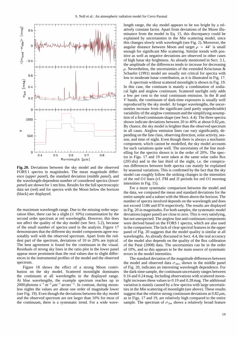
S. Noll et al.: An atmospheric radiation model for Cerro Paranal
Fig. 20. Deviations between the sky model and the observedFORS 1 spectra in magnitudes. The mean magnitude differ-ence (upper panel), the standard deviation (middle panel), andthe wavelength-dependent number of considered spectra (lowerpanel) are shown for 1 nm bins. Results for the full spectroscopicdata set (red) and for spectra with the Moon below the horizon(black) are displayed.
the maximum wavelength range. Due to the missing order sepa-ration filter, there can be a slight (<∼ 10%) contamination by thesecond order spectrum at red wavelengths. However, this doesnot affect the quality of the sky model (see Sect. 5.2), becauseof the small number of spectra used in the analysis. Figure 17demonstrates that the different sky model components agree rea-sonably well with the observed spectrum. Apart from the red-dest part of the spectrum, deviations of 10 to 20% are typical.The best agreement is found for the continuum in the visual.Residuals of strong sky lines in the ratio plot in the lower panelappear more prominent than the real values due to slight differ-ences in the instrumental profiles of the model and the observedspectrum.
Figure 18 shows the effect of a strong Moon contri-bution on the sky model. Scattered moonlight dominatesthe continuum at all wavelengths in the displayed range.At blue wavelengths, the example spectrum reaches up to2000 photons s−1 m−2 µm−1 arcsec−2. In contrast, during moon-less nights the values are about one order of magnitude lower(see Fig. 19). Even though the deviations between the sky modeland the observed spectrum are not larger than 10% for most ofthe continuum, there is a systematic trend. For a wide wave-
length range, the sky model appears to be too bright by a rel-atively constant factor. Apart from deviations of the Moon illu-minance from the model in Eq. 15, this discrepancy could beexplained by uncertainties in the Mie scattering model, sincethis changes slowly with wavelength (see Fig. 2). Moreover,theangular distance between Moon and targetρ = 44◦ is smallenough for significant Mie scattering. Similar trends with pos-itive as well as negative deviations are observed in other casesof high lunar sky brightness. As already mentioned in Sect. 3.1,the amplitude of the differences tends to increase for decreasingρ. Nevertheless, the uncertainties of the extended Krisciunas &Schaefer (1991) model are usually not critical for spectra withlow to moderate lunar contribution, as it is illustrated in Fig. 17.
A spectrum without scattered moonlight is shown in Fig. 19.In this case, the contiuum is mainly a combination of zodia-cal light and airglow continuum. Scattered starlight only addsa few per cent to the total continuum emission. In theB andV bands, the continuum of dark-time exposures is usually wellreproduced by the sky model. At longer wavelengths, the uncer-tainties increase from the significant (and partly unpredictable)variability of the airglow continuum and the simplifying assump-tion of a fixed continuum shape (see Sect. 4.4). The three spectrashown indicate deviations between 20 to 40% at about 0.82µm.By chance, the sky model is brighter than the observed spectrumin all cases. Airglow emission lines can vary significantly,de-pending on the line class, observing direction, solar activity, sea-son, and time of night. Even though there is always a stochasticcomponent, which cannot be modelled, the sky model accountsfor such variations quite well. The uncertainty of the line mod-elling for the spectra shown is in the order of 20%. The spec-tra in Figs. 17 and 19 were taken at the same solar radio flux(205 sfu) and in the last third of the night, i.e. the conspicu-ous differences between both spectra can mainly be explainedby seasonal variations. This is confirmed by the fact that theskymodel can roughly follow the striking changes in the intensitiesof the red O I lines (cf. FM and JJ periods for red O I morningintensities in Fig. 15).
For a more systematic comparison between the model andthe data, we computed the mean and standard deviations for theentire sample and a subset with the Moon above the horizon. Thenumber of spectra involved depends on the wavelength and doesnot exceed 1186 and 874 respectively. The results are displayedin Fig. 20 in magnitudes. For both samples, the systematic modeldeviations (upper panel) are close to zero. This is very satisfying,but not unexpected. The airglow line and continuum componentswere derived based on the FORS 1 spectra, which are also usedin the comparison. The lack of clear spectral features in theupperpanel of Fig. 20 suggests that the model quality is similar atallwavelengths. As already discussed in Sect. 4.4, the real accuracyof the model also depends on the quality of the flux calibrationof the Patat (2008) data. The uncertainties can be in the orderof 10%, and so this appears to be the main source of systematicerrors in the model intensities.
The standard deviation of the magnitude differences betweenthe model and observed dataσ∆m, shown in the middle panelof Fig. 20, indicates an interesting wavelength dependence. Forthe dark-time sample, the continuum uncertainty ranges between0.16 and 0.24 mag. Including observations with scattered moon-light increases these values to 0.19 and 0.28 mag. The additionalvariation is mainly caused by a few spectra with large uncertain-ties in the Mie scattering of moonlight (see above). These resultssuggest that the relative strong continuum deviations at 0.82µm,as in Figs. 17 and 19, are relatively high compared to the entiresample. The spectrum ofσ∆m shows a relatively broad feature
19

S. Noll et al.: An atmospheric radiation model for Cerro Paranal
at about 0.6µm, which is reminiscent of the shape of the FeOpseudo continuum (see Jennikens et al. 2000; Evans et al. 2010;Saran et al. 2011). This result supports the assumption thattheairglow continuum bump at 0.6µm (see Fig. 16) is mainly pro-duced by iron oxide (see Sect. 4.4) and varies differently thanthe underlying NO2 continuum, for which the intensitiy changesat 0.543µm are considered by the sky model. Fig. 20 indicatesa FeO-related variability of about 15%. Since the mean bumpcontributes about 20% of the total flux at 0.6µm, the variationis almost comparable to it. These strong variations are in agree-ment with previous results (see Evans et al. 2010; Saran et al.2011). A minor source of continuum variability at 0.6µm is theChappuis ozone bands (see Fig. 2), which indicate a variationof 0.02 mag airmass−1 (see Patat et al. 2011). The middle panelof Fig. 20 does not exhibit strong signatures of OH bands (seeFig. 13, panel 4). The bands are clearly detectable only in therange of low continuum uncertainty. Consequently, the qualityof the OH modelling is comparable or even better than the con-tinuum modelling. This is particularly important for the qual-ity of the full sky model at long wavelengths, where OH emis-sion dominates the spectra. The sky model is less able to modelatomic lines, as shown in Fig. 20. The maximum variability of0.7 mag is found at [O I] 6300. In addition, other lines of the ther-mospheric ionosphere, which are usually difficult to recognise(see Fig. 13, panel 3), significantly contribute toσ∆m. For exam-ple, N I at 520 nm and O I at 616, 656, and 777 nm are clearlydetectable. This confirms the conclusion of Sect. 4.3.2, statingthat the intensities of ionospheric lines are difficult to predictdue to their sensitivity to geomagnetic disturbances (see Roach& Gordon 1973).
5.2. Comparison of photometry
To perform a more quantitative comparison of our sky model andobserved data, and for an easier comparison to other studies, wederived magnitudes from broad-band filter fluxes. Specifically,we used the standard photometric system consisting ofU, B, V,R, andI (see Bessell 1990). For the Patat (2008) data and theircorresponding sky models, only a grism-dependent subset offil-ters can be taken. The spectrum needs to cover>∼ 90% of thefilter curve. An exception is theU filter, which extends below0.365µm, the lower wavelength limit of the bluest spectral set-up (see Sect. 4.2). Therefore, the results for this filter areques-tionable.
Figure 21 and Table 4 show the results of the computationsfor the full sample of FORS 1 spectra and a subsample with theMoon below the horizon (cf. Sect. 5.1). Only a small fraction(∼ 1/4) of the spectra contribute to the mean values and stan-dard deviations of theU and B filters. Most spectra cover therange of theV, R, andI filters. For both samples and all filters,the mean magnitude differences are small (<∼ 0.05 mag). Eventhough the sky model tends to be slightly fainter at the blue endand slightly brighter at the red end, there are no serious sys-tematic deviations from the observed spectra (cf. Sect. 5.1). Thestandard deviationsσ∆m are relatively similar for the differentfilters. For the full sample, they range from 0.19 mag for theV-band to 0.24 mag for theI band. Consequently, the accuracy ofthe sky model is in the order of about 20%. These values can becompared to the magnitude variations in the measured dataσobs,which correspond toσ∆m for an optimum sky model of time-invariant flux. For the full sample, the deviations are distinctlylarger. They range from 0.37 to 0.56 mag. These large deviationsare mainly due to the observations with a strong moonlight con-tribution (see Sect. 3.1). For dark-time conditions,〈∆m〉 ranges
Fig. 21. Histograms for the deviations of the sky model from theFORS 1 data in mag for the filtersU, B, V, R, andI. The filledhistograms show only data with the Moon above the horizon.
from 0.17 mag forB to 0.21 mag forU, andσ∆m indicates differ-ences between 0.18 mag forB and 0.29 mag forI. In particular,for the bandsV to I, a time-invariant sky model would be signifi-cantly worse than our sky model (see also Sect. 5.3). This showsthe improvements from a variable zodiacal light, airglow lines,and airglow continuum model.
Finally, we compare the sky model to literature data.Magnitudes in the five broad-band filtersU to I were calculatedusing standardised observing conditions. Specifically, zenith,New Moon, ecliptic pole, annual average, and mean solar ac-tivity, i.e. 130 sfu (see Sect. 4.3.2), were assumed. The resultingmagnitudes are provided in Table 5. For a better comparison withpublished data, the table also contains sky model results for 90and 180 sfu. The reference data in Table 5 originate from Mattilaet al. (1996) for La Silla, Walker (1987) and Krisciunas et al.(2007) for Cerro Tololo, Benn & Ellison (1998) for La Palma,and Patat (2003, 2008) for Cerro Paranal. In general, there is agood agreement between the sky model and observed sky bright-nesses. By comparing magnitudes with similar average solarra-dio fluxes, we find typical deviations in the order of 0.1 mag.An exception is theU filter with typical differences of about0.3 mag, which could be explained by the lower quality of thesky model at near-UV wavelengths due to the lack of data (seeSect. 4.2). Also, it is not clear to what extent components like zo-diacal light or scattered starlight, which significantly affect shortwavelengths, contribute to the observed data. The corresponding
20
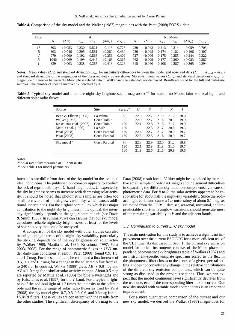
S. Noll et al.: An atmospheric radiation model for Cerro Paranal
Table 4. Comparison of the sky model and the Walker (1987) magnitudeswith the Patat (2008) FORS 1 data.
Filter All No MoonN 〈∆m〉 σ∆m σobs 〈∆mw〉 σ∆m,w N 〈∆m〉 σ∆m σobs 〈∆mw〉 σ∆m,w
U 303 +0.053 0.230 0.521 −0.113 0.725 239 +0.042 0.213 0.214 −0.059 0.703B 303 +0.046 0.205 0.561 +0.269 0.430 239 +0.048 0.174 0.182 +0.196 0.407V 979 +0.000 0.192 0.563 +0.356 0.409 727 +0.006 0.175 0.255 +0.244 0.322R 1046 +0.009 0.199 0.447 +0.169 0.365 762 −0.009 0.177 0.260 +0.083 0.287I 839 −0.003 0.238 0.365 +0.413 0.326 615 −0.040 0.208 0.287 +0.365 0.294
Notes. Mean values〈∆m〉 and standard deviationsσ∆m for magnitude differences between the model and observed data (∆m = mmodel− mobs)and standard deviations of the magnitudes of the observed dataσobs are shown. Moreover, mean values〈∆mw〉 and standard deviationsσ∆m,w formagnitude differences between the Moon phase related data of Walker and thePatat data are displayed. Results are listed for the full anddark-timesamples. The number of spectra involved is indicated byN.
Table 5. Typical sky model and literature night-sky brightnesses inmag arcsec−2 for zenith, no Moon, faint zodiacal light, anddifferent solar radio fluxes.
Source Site S 10.7 cma U B V R I
Benn & Ellison (1998) La Palma 80 22.0 22.7 21.9 21.0 20.0Walker (1987) Cerro Tololo 90 22.0 22.7 21.8 20.9 19.9Krisciunas et al. (2007) Cerro Tololo 130 22.1 22.8 21.8 21.219.9Mattila et al. (1996) La Silla 150 22.8 21.7 20.8 19.5Patat (2008) Cerro Paranal 160 22.4 22.7 21.7 20.9 19.7Patat (2003) Cerro Paranal 180 22.3 22.6 21.6 20.9 19.7
Sky modelb Cerro Paranal 90 22.3 22.9 22.0 21.2 19.8130 22.1 22.8 21.8 21.0 19.7180 21.9 22.6 21.6 20.9 19.6
Notes.(a) Solar radio flux measured at 10.7 cm in sfu.(b) See Table 1 for model parameters.
intensities can differ from those of the sky model for the assumedideal conditions. The published photometry appears to confirmthe lack of reproducibility ofU-band magnitudes. Unexpectedly,the sky brightness seems to increase with decreasing solar activ-ity. It should be noted that photometric samples are often toosmall to cover all of the airglow variability, which causes addi-tional uncertainties. For the airglow continuum, which is amajorcontribution to the night-sky brightness in the optical, the inten-sity significantly depends on the geographic latitude (see Davis& Smith 1965). In summary, we can assume that our sky modelcalculates reliable night-sky brightnesses, at least for the levelsof solar activity that could be analysed.
A comparison of the sky model with other studies can alsobe enlightening in terms of the night-sky variability, particularlythe striking dependence of the sky brightness on solar activ-ity (Walker 1988; Mattila et al. 1996; Krisciunas 1997; Patat2003, 2008). For the range of photometric fluxes inUVI un-der dark-time conditions at zenith, Patat (2008) found 0.9,1.3,and 1.7 mag. For the same filters, he estimated a flux increase of0.6, 0.3, and 0.2 mag for a change in the solar radio flux from 80to 240 sfu. In contrast, Walker (1988) gives∆B ≈ 0.8 mag and∆V ≈ 1.0 mag for a similar solar activity change. About 0.5 magare reported by Mattila et al. (1996) for blue wavelengths andby Krisciunas et al. (1997) for theV band. For a typical bright-ness of the zodiacal light of 1.7 times the intensity at the eclipticpole and the same range of solar radio fluxes as used by Patat(2008), the sky model gives 0.7, 0.5, 0.6, 0.6, and 0.3 mag fortheUBVRI filters. These values are consistent with the results fromthe other studies. The significant discrepancy of 0.3 mag to the
Patat (2008) result for theV filter might be explained by the rela-tive small sample of only 148 images and the general difficultiesin separating the different sky radiation components by means ofphotometric data. ForB to R, the solar activity appears to be re-sponsible for about half the night-sky variability. Since the zodi-acal light variations cause a 1σ uncertainty of about 0.1 mag, asestimated from the FORS 1 data set, seasonal, nocturnal, andun-predictable short-term airglow variations should generate mostof the remaining variability inV and the adjacent bands.
5.3. Comparison to current ETC sky model
The main motivation for this study is to achieve a significantim-provement over the current ESO ETC for a more efficient use ofthe VLT time. As discussed in Sect. 1, the current sky emissionmodel for optical instruments consists of the Moon phase de-pendent, photometric sky brightness table of Walker (1987)andan instrument-specific template spectrum scaled to the flux inthe photometric filter closest to the centre of a given spectral set-ting. It does not consider any change in the relative contributionsof the different sky emission components, which can be quitestrong as discussed in the previous sections. Thus, we can ex-pect that the model continuum level significantly deviates fromthe true one, even if the corresponding filter flux is correct.Ournew sky model with variable model components is an importantimprovement.
For a more quantitative comparison of the current and ournew sky model, we derived the Walker (1987) magnitudes for
21
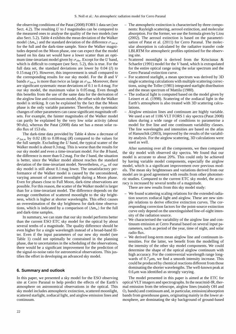
S. Noll et al.: An atmospheric radiation model for Cerro Paranal
the observing conditions of the Patat (2008) FORS 1 data set (seeSect. 4.2). The resultingU to I magnitudes can be compared tothe measured ones to analyse the quality of the two models (seealso Sect. 5.2). Table 4 exhibits the mean deviation of the Walkermodel〈∆mw〉 and the standard deviation of the differenceσ∆m,wfor the full and the dark-time sample. Since the Walker magni-tudes depend on the Moon phase, one can expect that the modelbased on his data set would have a lower scatter than an opti-mum time-invariant model given byσobs. Except for theU band,which is difficult to compare (see Sect. 5.2), this is true. For thefull data set, the standard deviations are lower by 0.04 (I) to0.15 mag (V). However, this improvement is small compared tothe corresponding results for our sky model. For theB andVbandsσ∆m,w is more than twice as large asσ∆m. Moreover, thereare significant systematic mean deviations of 0.1 to 0.4 mag.Forour sky model, the maximum value is 0.05 mag. Even thoughthis benefits from the use of the same data for the derivation ofthe airglow line and continuum model, the offset with the Walkermodel is striking. It can be explained by the fact that the Moonphase is the only variable parameter. Therefore, the systematicchanges of other parameters can cause significant magnitudeoff-sets. For example, the fainter magnitudes of the Walker modelcan partly be explained by the very low solar activity (about90 sfu), whereas the Patat (2008) data set has a mean solar ra-dio flux of 153 sfu.
The dark-time data provided by Table 4 show a decrease ofσ∆m,w by 0.02 (B) to 0.08 mag (R) compared to the values forthe full sample. Excluding theU band, the typical scatter of theWalker model is about 0.3 mag. This is worse than the results forour sky model and even a time-invariant model. For theB band,the difference is more than 0.2 mag. For theI band, the situationis better, since the Walker model almost reaches the standarddeviation of the time-invariant model. Nevertheless,σ∆m of oursky model is still about 0.1 mag lower. The unsatisfactory per-formance of the Walker model is caused by the unconsidered,varying amount of scattered moonlight during a Moon phase.Even for phases close to Full Moon, dark-time observations arepossible. For this reason, the scatter of the Walker model islargerthan for a time-invariant model. The difference depends on theaverage contribution of scattered moonlight to the sky bright-ness, which is higher at shorter wavelengths. This effect causesan overestimation of the sky brightness for dark-time observa-tions, which is indicated by a comparison of〈∆mw〉 for the fulland dark-time samples.
In summary, we can state that our sky model performs betterthan the current ESO ETC sky model for the optical by aboutseveral tenths of a magnitude. The quality difference should beeven higher for a single wavelength instead of a broad-band fil-ter. Even if the input parameters of our new sky model (seeTable 1) could not optimally be constrained in the planningphase, due to uncertainties in the scheduling of the observations,there would be a significant improvement for the prediction ofthe signal-to-noise ratio for astronomical observations.This jus-tifies the effort in developing an advanced sky model.
6. Summary and outlook
In this paper, we presented a sky model for the ESO observingsite at Cerro Paranal to help predict the effects of the Earth’satmosphere on astronomical observations in the optical. Thissky model includes atmospheric extinction, scattered moonlight,scattered starlight, zodiacal light, and airglow emissionlines andcontinuum.
– The atmospheric extinction is characterised by three compo-nents: Rayleigh scattering, aerosol extinction, and molecularabsorption. For the former, we use the formula given by Liou(2002). The aerosol extinction is based on the parametri-sation of Patat et al. (2011) for Cerro Paranal. The molec-ular absorption is calculated by the radiative transfer codeLBLRTM for atmospheric profiles optimised for the observ-ing site.
– Scattered moonlight is derived from the Krisciunas &Schaefer (1991) model for theV band, which is extrapolatedfor the entire optical range using the solar spectrum and theCerro Paranal extinction curve.
– For scattered starlight, a mean spectrum was derived by 3Dsingle scattering calculations with multiple scattering correc-tions, using the Toller (1981) integrated starlight distributionand the mean spectrum of Mattila (1980).
– The zodiacal light is computed based on the model given byLeinert et al. (1998). Scattering of the zodiacal light in theEarth’s atmosphere is also treated with 3D scattering calcu-lations.
– Airglow emission lines and continuum are highly variable.We used a set of 1186 VLT FORS 1 sky spectra (Patat 2008)taken during a wide range of conditions to parametrise amodel for five line and one continuum variability classes.The line wavelengths and intensities are based on the atlasof Hanuschik (2003), improved by the results of the variabil-ity analysis. For the airglow scattering, 3D calculations wereused as well.
After summing over all the components, we then comparedthe sky model with observed sky spectra. We found that ourmodel is accurate to about 20%. This could only be achievedby having variable model components, especially the airglowmodel, which is a significant improvement over previous mod-els. The mean sky brightnesses and variations derived from ourmodel are in good agreement with results from other photomet-ric studies. Compared to the current ETC sky model, the accu-racy is increased by several tenths of a magnitude.
There are new results from this sky model study:
– We found scattering scaling relations for the extended radia-tion sources zodiacal light and airglow. These are new sim-ple relations to derive effective extinction curves. The cor-responding correction factors for the point-source extinctioncurve only depend on the unextinguished line-of-sight inten-sity of the radiation source.
– We characterised the variability of the airglow line and con-tinuum emission at Cerro Paranal based on several input pa-rameters, such as period of the year, time of night, and solarradio flux.
– We derived long-term mean airglow line and continuum in-tensities. For the latter, we benefit from the modelling ofthe intensity of the other sky model components. We coulddetermine the shape of the optical airglow continuum withhigh accuracy. For the controversial wavelength range long-wards of 0.7µm, we find a smooth intensity increase. Thiscould be produced by chemical reactions different from thosedominating the shorter wavelengths. The well-known peak at0.6µm was identified as strongly varying.
The model presented in this paper is aimed at the ETC foroptical VLT imagers and spectrographs. In the near/mid-IR, ther-mal emission from the telescope, airglow lines (mainly OH andO2 bands) and continuum and, in particular, emission/absorptionbands from greenhouse gases, originating mainly in the lower at-mosphere, are dominating the sky background of ground-based
22

S. Noll et al.: An atmospheric radiation model for Cerro Paranal
observations. The scattering-related components become negli-gible. The change in significance between the components aswell as the necessity to use IR data sets for the analysis requiresdifferent modelling techniques to achieve reliable ETC predic-tions in the IR. The IR sky radiation model will be described ina forthcoming paper.
The sky model can also be used as a basis for proceduresaiming at reconstructing data by removing the sky signature.This purpose requires the adaption of the sky model to enablethe fitting of observed data. Preliminary studies show promisingresults for this kind of application, which will also be presentedin future papers.
Acknowledgements. We are indebted to F. Patat for providing his FORS 1 dataset and his LBLRTM set-up for the calculation of the best-fit Paranal extinctioncurve. We thank A. Seifahrt for his support and helpful comments on the use ofLBLRTM and the creation of suitable atmospheric profiles. Weare grateful toR. Hanuschik for making his UV spectra available to us. Thanks also go to P.Ballester for his input to the paper and his prudent management of the projecton ESO side and A. Smette for fruitful discussions. Finally,we thank the anony-mous referee for his detailed and helpful comments. This study was carried out inthe framework of the Austrian ESO In-Kind project funded by BM:wf under con-tracts BMWF-10.490/0009-II/10/2009 and BMWF-10.490/0008-II/3/2011. Thispublication is also supported by the Austrian Science Fund (FWF).
References
Ashburn, E.V. 1954, J. Atmos. Terr. Phys., 5, 83Baldwin, J.A., & Stone, R.P.S. 1984, MNRAS, 206, 241Ballester, P., Pizarro De La Iglesia, J.A., Modigliani, A.,& Boitquin, O. 2000,
in ASP Conference Series, Vol. 216, Astronomical Data Analysis Softwareand Systems IX, eds. N. Manset, C. Veillet, & D. Crabtree, (San Francisco:Astronomical Society of the Pacific), 331
Barth, C.A., & Hildebrand, A.F. 1961, J. Geophys. Res., 66, 985Bates, D.R., & Nicolet, M. 1950, J. Geophys. Res., 55, 301Bates, D.R. 1982. In: Applied atomic collision physics, Atmospheric physics and
chemistry, Vol. 1, Academic Press, New York, 149Benn C.R., & Ellison, S.L. 1998, La Palma technical note, 115Bernstein, R.A., Freedman, W.L., & Madore, B.F. 2002, ApJ, 571, 85Bessell, M.S. 1990, PASP, 102, 1181Burki, G., Rufener F., Burnet, M., et al. 2005, A&AS, 112, 383Chamberlain, J.W. 1961, Physics of the Aurora and Airglow, Academic Press,
New YorkChapman, S. 1939, ApJ, 90, 309Clough, P.N., & Thrush, B.A. 1967, Trans. Faraday Soc. 63, 915Clough, S.A, Shephard, M.W., Mlawer. E.J., et al. 2005, J. Quant. Spectrosc.
Radiat. Transfer, 91, 233Colina, L., Bohlin, R.C., & Castelli, F. 1996, AJ, 112, 307Content, R. 1996, ApJ, 464, 412Cosby, P.C., Sharpee, B.D., Slanger, T.G., Huestis, D.L., &Hanuschik, R.W.
2006, J. Geophys. Res., 111, A12307Covington, A.E. 1969, JRASC, 63, 125Cuby, J.G., Lidman, C., & Moutou, C. 2000, The Messenger, 101, 2Dave, J.V. 1964, J. Opt. Soc. America, 54, 307Davies, R.I. 2007, MNRAS, 375, 1099Davis, T.N., & Smith, L.L. 1965, J. Geophys. Res., 70, 1127Edlen, B. 1966, Metrologia, 2, 71Ellis, S.C., & Bland-Hawthorn, J. 2008, MNRAS, 386, 47Elterman, L. 1996, Appl. Optics, 5, 1769Evans, W.F.J., Gattinger, R.L., Slanger, T.G., et al. 2010,Geophys. Res. Lett.,
37, L22105Green, A.E.S., Deepak, A., & Lipofsky, B.J. 1971, Appl. Optics, 10, 1263Gutierrez-Moreno, A., Moreno, A., & Cortes, G. 1982, PASP, 94, 722Gutierrez-Moreno, A., Moreno, A., & Cortes, G. 1986, PASP, 98, 1208Hanuschik, R.W. 2003, A&A, 407, 1157Jenniskens, P., Lacey, M., Allan, B.J., Self, D.E., & Plane,J.M.C. 2000, Earth
Moon Planets, 82/83, 429Kenner, R.D., & Ogryzlo, E.A. 1984, J. Chem. Phys., 80, 1Khomich, V.Y, Semenov, A.I., & Shefov, N.N. 2008, Airglow asan Indicator of
Upper Atmospheric Structure and Dynamics, Springer, BerlinKrisciunas, K. 1997, PASP, 109, 1181Krisciunas, K., & Schaefer, B.E. 1991, PASP, 103, 1033Krisciunas, K., Semler, D.R., Richards, J., et al. 2007, PASP, 119, 687Krassovsky, V.I. 1951, Dokl. Akad. Nauk SSSR, 78, 669Levasseur-Regourd, A.-C., & Dumont, R. 1980, A&A, 84, 277
Leinert, C., Bowyer, S., Haikala, L.K., et al. 1998, A&AS, 127, 1Liou, K.-N. 2002, Introduction to Atmospheric Radiation, Second Edition,
Academic Press, San DiegoLiu, G., & Shepherd, G.G. 2008, Adv. Space Res., 42, 933Mattila, K. 1980, A&AS, 39, 53Mattila, K. 2003, ApJ, 591, 119Mattila, K., Vaisanen, P., & von Appen-Schnur, G.F.O. 1996, A&AS, 119, 153Meinel, A.B., Negaard, B.J., & Chamberlain, J.W. 1954, J. Geophys. Res., 59,
407Melchior, A.-L., Combes, F., & Gould, A. 2007, A&A, 462, 965Nicolet, M. 1989, Planet. Space Sci., 37, 1249Noll, S., Burgarella, D., Giovannoli, E., et al. 2009, A&A, 507, 1793Patat, F. 2003, A&A, 400, 1183Patat, F. 2008, A&A, 481, 575Patat, F., Moehler, S., O’Brien, K., et al. 2011, A&A, 527, A91Roach, F.E., & Gordon J.L. 1973, The light of the night sky, Reidel, DordrechtRothman, L.S., Gordon, I.E., Barbe, A., et al. 2009, J. Quant. Spectrosc. Radiat.
Transfer, 110, 533Rousselot, P., Lidman, C., Cuby, J.-G., Moreels, G., & Monnet, G. 2000, A&A,
354, 1134Rozenberg, G.V. 1966. Twilight: A Study in Atmospheric Optics, New York:
Plenum Press, 160Rufener, F. 1986, A&A, 165, 275Saran, D.V., Slanger, T.G., Feng, W., & Plane, J.M.C. 2011, J. Geophys. Res.,
116, D12303Seifahrt, A., Kaufl, H.U., Zangl, G., et al. 2010, A&A, 524,A11Sobolev, V.G. 1978, Planet. Space Sci., 26, 703Staude, H.J. 1975, A&A, 39, 325Sterken, C., & Manfroid, J. 1992, A&A, 266, 619Sternberg, J.R., & Ingham, M.F. 1972, MNRAS, 159, 1Stone, R.P.S., & Baldwin, J.A. 1983, MNRAS, 267, 904Toller, G.N. 1981, Ph.D. Dissertation, State University ofN.Y. at Stony BrookToller, G.N., Tanabe, H., & Weinberg, J.L. 1987, A&A, 188, 24Tug, H. 1977, Messenger, 11, 7Tug, H. 1980, A&A, 82, 195van Rhijn, P.J. 1921, Publ. Astr. Lab. Groningen, 31, 1von Savigny, C.H.A., McDade, I.C., Shepherd, G.G., & Rochon, Y. 1999, Ann.
Geophys., 17, 1439Walker, A. 1987, NOAO Newsletter, 10, 16Walker, M.F. 1988, PASP, 100, 496West, J.B., & Broida, H.P. 1975, J. Chem. Phys., 62, 2566Wolstencroft, R.D., & van Breda, I.G. 1967, ApJ, 147, 255
23


![Las Leñas Valley,Cerro General Carrera, north face; Cerro Manuel Rodríguezpublications.americanalpineclub.org/articles/13201213191.pdf · [3,313m, GPS]), and Cerro Manuel Rodríguez](https://static.fdocuments.in/doc/165x107/5f05ebae7e708231d415627f/las-leas-valleycerro-general-carrera-north-face-cerro-manuel-rodr-3313m.jpg)


