An Assessment of Land Cover Changes Using GIS and

Remote Sensing:

A Case Study of the uMhlathuze Municipality,

KwaZulu-Natal, South Africa

by

Thomas Forster Robson

Submitted as the dissertation component in partial fulfilment of the

requirements for the degree of Master of Environment and Development in

the Centre for Environment, Agriculture and Development, School of

Environmental Science, University of KwaZulu-Natal

Pietermaritzburg

June, 2005

ABSTRACT

Rapid growth of cities is a global phenomenon exerting much pressure on land resources and

causing associated environmental and social problems. Sustainability of land resources has

become a central issue since the Earth Summit in Rio de Janeiro in 1992. A better

understanding of the processes and patterns of land cover change will aid urban planners and

decision makers in guiding more environmentally conscious development. The objective of

this study was firstly, to determine the location and extent of land use and land cover changes

in the uMhlathuze municipality, KwaZulu-Natal, South Africa between 1992 and 2002, and

secondly, to predict the likely expansion of urban areas for the year 2012. The uMhlathuze

municipality has experienced rapid urban growth since 1976 when the South African Ports and

Railways Administration built a deep water harbour at Richards Bay, a town within the

municipality. Three Landsat satellite images were obtained for the years, 1992, 1997 and

2002. These images were classified into six classes representing the dominant land covers in

the area. A post classification change detection technique was used to determine the extent and

location of the changes taking place during the study period. Following this, a GIS-based land

cover change suitability model, GEOMOD2, was used to determine the likely distribution of

urban land cover in the year 2012. The model was validated using the 2002 image. Sugarcane

was found to expand by 129% between 1992 and 1997. Urban land covers increased by an

average of 24%, while forestry and woodlands decreased by 29% between 1992 and 1997.

Variation in rainfall on the study years and diversity in sugarcane growth states had an impact

on the classification accuracy. Overall accuracy in the study was 74% and the techniques gave

a good indication of the location and extent of changes taking place in the study site, and show

much promise in becoming a useful tool for regional planners and policy makers.

PREFACE

The experimental work described in this dissertation was carried out in the Centre for Environment,

Agriculture and Development, School ofEnvironmental Science, University of KwaZulu-Natal,

Pietermaritzburg Campus, fro m August 2004 to June 2005 under the supervision ofDr Trevor Hill and

Dr Fethi Ahmed.

These studies represent the original work by the author and have not otherwise been submitted in any

form for any degree or diploma to any University. Where use has been made of the work of others it is

duly acknowledged in the text.

This dissertation is divided into Component A and Component B. Component A contains an

introduction, a summary of the study site, a literature review and a description of the methods used.

Component B is written in the format of a journal paper prepared for the journal; Remote sensing of

Environment. As specified by the Journal, the majority of the figures are presented in black and white.

Signed

Thomas F. Robson

Signed

Dr Fethi Ahmed

It I!...l. j1 .Signed

Dr Trevor Hill

Date

...\1.l ~ ~.t.V!J).} .Date

...#/P.4.f.?q~~.: .Date

Il

TABLE OF CONTENTS

ABSTRACT _

PREFACE ii

TABLE OF CONTENTS iii

LIST OF FIGURES vi

LIST OF TABLES vii

LIST OF ABBREVIATIONS viii

ACKNOWLEDGEMENTS ix

CHAPTER 1. INTRODUCTION 1

1.1. Introduction 1

1.2. The Importance of Land 2

1.3. Land Uses and Land Covers 3

1.4. Aims and Objectives 4

1.5. Summary 5

CHAPTER 2. STUDY SITE 7

2.1. The uMhlathuze Municipality 7

2.2. The Natural Environment 8

2.3. History of the uMhlathuze Municipality 11

2.4. Development Strategies and Government Policies 12

2.5. Summary 14

CHAPTER 3. LITERATURE REVIEW 16

3.1. Ecological Urban Dynamics and Environmental Considerations 16

3.1.1. Urban Expansion and Population Growth 16

III

3.1.2.

3.1.3.

Urban Ecosystems 18

Urban Open Space 20

3.5.3.

3.5.4.

3.5.5.

3.5.6.

3.5.7.

3.5.8.

3.2. The Role of GIS and Remote Sensing in Land Use and Land Cover Change_ 21

3.2.1. The Benefits and Limitations of GIS 22

3.2.2. The Benefits and Limitations of Remote Sensing 23

3.2.3. Landsat Satellite Imagery 24

3.3. Determinants of Land Use and Land Cover Change 25

3.3.1. Economic Factors 27

3.3.2. Social Factors 27

3.3.3. Spatial Interactions and Neighbourhood Characteristics 28

3.3.4. Biophysical Factors 28

3.3.5. Policy Factors 28

3.3.6. Sugarcane Expansion 29

3.4. Land Use and Land Cover Change Detection 30

3.4.1. The Importance of Change Analysis 30

3.4.2. Data Preprocessing 31

3.4.3. Image Classification 32

3.4.4. Classification Accuracy Assessment 35

3.4.5. Change Detection Techniques 36

3.4.6. Post Classification Comparison 38

3.5. Modelling Land Cover Change and Urban Landscape Dynamics 39

3.5.1. Introduction 39

3.5.2. The Development of Land Use and Land Cover Change (LUCC) and Urban

Landscape Models 40

Cellular Automata Models 41

Markov Chain Models 43

Common Land Use and Cover Change (LUCC) Models 45

GEOMOD2 46

Model Validation 48

Recent Developments in Urban Modelling 49

iv

3.6. Summary 51

CHAPTER 4. METHODS 52

4.1. Introduction 52

4.2. Data 52

4.2.1. Satellite Imagery 52

4.2.2. Data Preprocessing 52

4.3. Change Detection 54

4.3.1. Image Classification 54

4.3.2. Accuracy Assessment 60

4.3.3. Change Detection 62

4.4. Land Use and Land Cover Change Modelling 62

4.4.1. Creation of the Suitability Image 63

4.4.2. GEOMOD2 64

4.4.3. Model Validation 65

4.5. Summary 66

REFERENCES 67

APPENDICES 75

v

LIST OF FIGURES

Figure 2-1 Location of urban areas, settlements and lakes within the uMhlathuze municipality 7

Figure 2-2 Wetland area with large Industries in the background 9

Figure 2-3 Grassland area situated between large industrial areas in Richards Bay 10

Figure 2-4 Map of the broad land use zones in Richards Bay 14

Figure 3-1 Diagrammatic illustration of the class allocation method of the 'parallelepiped'

decision rule (taken from Eastman, 2001) 33

Figure 3-2 Diagrammatic illustration of the class allocation method of the 'minimum distance

to means' decision rule (taken from ERDAS, Inc, 1997) 34

Figure 3-3 Diagrammatic illustration of the class allocation method of the 'maximum

likelihood' decision rule (taken from Eastman, 2001) 35

Figure 3-4 Transition process of a generic cellular automaton (taken from Leao et al., 2004) .43

Figure 3-5 Diagrammatic representation of GEOMOD2 land use and land cover change model

(adapted from Pontius et al., 2001) 47

Figure 4-1 Flowchart of the steps undertaken during the preprocessing stage 54

Figure 4-2 Landsat-5 image of study site in 1992 viewed through a combination of bands 2

(green), 3 (red) and 4 (near infrared) 55

Figure 4-3 Landsat-7 image of study site in 1997 viewed through a combination of bands 2

(green), 3 (red) and 4 (near infrared) 55

Figure 4-4 Landsat-7 image of study site in 2002 viewed through a combination of bands 2

(green), 3 (red) and 4 (near infrared) 56

Figure 4-5 Spectral profiles of the 11 broad land cover classes in the study area, taken from the

1992 image 56

Figure 4-6 Flow chart of the steps undertaken during the classification process 60

Figure 4-7 Location of the ground truth points used in the accuracy assessment. 61

Figure 4-8 Flowchart of the steps undertaken during the predictive modelling section 65

Vi

LIST OF TABLES

Table 3-1 Landsat-5 band wavelengths 24

Table 3-2 Landsat-7 Characteristics 25

Table 3-3 Brief description of some of the more common LUCC models .45

Table 4-1 Description ofland cover classes used in the study 57

Table 4-2 Broad classification classes with sub-classes 58

Table 4-3 Number ofpixels under built-up land during the relevant years 64

vu

UNPDGISSLEUTHLUCC ModelsUSGSIDPMOSSSDIGEARSMEsCTCUNPDNASAETM+CRPSGDTCVAPCAGSEMITLUPCACLUEANNLEAMSMEKno

Klocation

Kquality

Kstandard

VPILVPIQMAS/LUCCUGMCURBASDSSTMSPOTNOAAAVHRRMODISGPSMCE

LIST OF ABBREVIATIONS

- United Nations Population Division- Geographical Information Systems- Slope, Land cover, Exclusion, Urbanisation, Transport and Hillshade- Land Use and Land Cover Change Models- United states Geological Survey- Integrated Development Planning- Metropolitan Open Space System- Spatial Development- Growth Employment and Redistribution- Small and Medium Enterprises- Central Timber Corporation- United Nations Population Division-National Aeronautics and Space Administration- Enhanced Thematic Mapper Plus- Conservation Reserve Program- Small Grower Development Trust- Change Vector Analysis- Principal Component Analysis- Gramm-Schmidt- Expectation-Maximisation- Integrated Transportation and Land-Use Package- Cellular Automata- Changing Land Use and Estuaries Model- Artificial Neutral Networks- Landuse Evolution and Impact Assessment Model- Spatial Modelling Environment- Kappa for no information- Kappa for location- Kappa for quality- standard Kappa- Value of Perfect Information of Location- Value of Perfect Information of Quantity- Multi-Agent System Model of Land-Use/Cover Change- Urban Growth Model- California Urban and Biodiversity Analysis- Spatial Decision Support System- Thematic Mapper- Systeme Probatoire d'Observation de la Terre- National Oceanic and Atmospheric Administration-Advanced Very High Resolution Radiometer- Moderate Resolution Imaging Spectroradiometer- Global Positioning System- Multi-Criteria Evaluation

Vlll

ACKNOWLEDGEMENTS

I would firstly like to thank my two supervisors Dr Fethi Ahmed and Dr Trevor Hill for their

contributions and supervision.

Secondly, I would also like to thank Mr Dechlan Pillay of the CSIR for kindly organising and

preprocessing the satellite imagery used in the study.

Thanks must also go to;

• The Satellite Applications Centre (SAC) for providing me with the data.

• Craven Naidoo and Brice Gijbertsen in the Cartography unit for their help with maps

and software.

• Mr Carel Bezuidenhoud & Mr Tom Fortman for their help and expertise.

IX

CHAPTER 1. INTRODUCTION

1.1. Introduction

"To understand how urban ecosystems work and to achieve ecological sustainability

in urban areas, we must be able to quantify and project land use and land cover

change and its ecological consequences" (Wu et al., 2003).

Rapid growth of cities is a global phenomenon, particularly pertinent to the Third World

(United Nations Population Division, 2002). This growth exerts much pressure on the land and

resources surrounding a city and has associated environmental and social problems.

Development needs to take place in a manner sensitive to such impacts. Thus to plan and

manage development appropriately and suitably, one needs to understand the process of urban

growth and the impacts of land use and land cover changes.

Changes in land uses and land covers take place in response to human needs and wants and are

a consequence of a range of factors stemming from many different disciplines, interlinking to

provide the existing patterns. Such factors need to be understood in order to determine the

impacts of such changes (Verburg et al., 1999). The impacts are usually significant in

economic, social and environmental terms and consequently have significant implications for

a range of policy issues including the management of urban areas, protection of wildlife

habitats and mitigation of global climate change (Lubowski et al., 2003). Policy is frequently

formulated in response to changes as a way of reducing or regulating the negative impacts of

changes and as such policy makers need to be kept well informed of the changes taking place.

Governments have an obligation to create, update and implement laws and policies regarding

current and future uses of land. Such decisions need to be based on a sound knowledge of the

current and past land use patterns as these will demonstrate the trajectory of change over time

and allow one to estimate the most likely future trends with improved confidence. Readily

1

available data of land use and land cover changes would allow planners to implement

appropriate strategies.

Various models and techniques have been created to provide information on such changes.

Verburg et al. (in press) describe Land Use and Land Cover Change (LUCC) models as tools

designed to support the analysis of the causes and consequences of land use dynamics in order

to improve our understanding of the processes of the land use system and to aid land use

planning and policy. Models have proved to be a successful way of understanding complex

interactions between the socio-economic and biophysical forces that impact the rate and

spatial arrangement of land use and land coverchange and for calculating the impacts of land

use and land cover change (Muller & Middleton 1994; Brown et al., 2000; Wu & Webster

2000; Weng 2002; Barredo et al., 2004; Leao et al., 2004; Verburg et al., 1999, in press).

The capability and accuracy of models is constantly increasing as they are developed and

modified. With growing application, LUCC models are becoming a valuable tool providing

planners and policy makers with important information to make better informed decisions.

1.2. The Importance of Land

Land is the basic natural resource from which humans draw most of their sustenance, fuel and

shelter (Mather, 1989). In addition, it provides a biophysical resource base for the production

of biological products such as food and fodder, and raw materials for people, livestock and

industry (Bonte-Friedmein & Kassam, 1994). It is also a source of biodiversity, minerals,

fossils, renewable energy and other natural resources that contribute to the wealth of human

life.

Human population growth has, and is continuing to place enormous pressure on this resource.

As populations grow, so too does the living space required and more importantly, the

agricultural land required to produce enough food, and other space required to produce

consumable products required by the population. It is thus imperative to acknowledge the

importance of policy to promote more sustainable land use strategies (Deal, 2001).

2

Land is a vital resource in terms of regulating the climate and natural environment. Changes in

land use and land cover affect the climate, the hydrological cycle, nutrient cycling and many

other important services provided by the land (Bonte-Friedmein & Kassam, 1994). Without

regulation on access and use of land such system will inevitably break down having serious

consequences for all living beings.

1.3.Land Uses and Land Covers

Knowledge of land uses is fundamental for socio-economic planning such as the placement of

new schools and services, and for the allocation of appropriate income tax rates (Verburg et

al., 2004). Land cover knowledge is important for such studies as rainfall runoff

characteristics, soil loss, habitat distribution and agricultural planning (Campbell, 1983).

Similarly, changes in land use and land cover have large impacts on large scale ecological and

environmental systems and must be incorporated into policy to address problems such as

urbanisation, global climate change, desertification and resource management (Wu et al.,

2003). Furthermore, Lillesand & Kiefer (1994) consider a good understanding of land use and

land cover to be vital for modelling the earth as a system.

Land cover describes the types of features present on the surface of the earth (Lillesand &

Kiefer, 1994) or as Kivel (1991) describes it, the nature of the elements of the landscape. The

land cover, in effect, represents either the vegetative cover of the land whether it is natural or

human generated, or the visible evidence of the land use (Campbell, 1983). It has no emphasis

on the economic function of the area. Land use has been defined as "the use of land by

humans, usually with emphasis on the functional role of land in economic activities"

(Campbell, 1983: 8). Due to the wide range of objectives of land use studies, no single

definition is best in all contexts. The land use of an area is not necessarily represented by the

visible cover of the land but is usually associated with some sort of visible cover or artefacts

present that are representative of a particular land use. Land use has often been subdivided into

urban and rural classes for the sake of clarity.

3

The definition of the term 'urban' is another subject that has undergone much discussion and

is important to this research. Some of the more common methods of defining the term

include; the imposition of a population size threshold, consideration of continuous built-up

areas covered by buildings and urban structures and the spatial distribution of city functions

(Campbell, 1983). Others have used a residual urban definition from agricultural surveys or

have attempted to define the rural urban boundary though statistical techniques (Kivel, 1991).

A further aspect of land that requires mention is that it varies greatly in quality and suitability

for different purposes. Thus, the characteristics of land can provide valuable information

regarding land uses and changes in land uses (Coppock, 1991). Aspects such as relief, 1 in 50

year flood lines, soil conditions and proximity to favourable/unfavourable areas can all limit

the range of land uses available to a particular site. There are several land use and land cover

classification systems used today such as that developed by the United States Geological

Survey (USGS) (Anderson 1976), the National Land Use Classification (NLUC) used in

Britain and the Standard Land-Cover Classification Scheme used in South Africa (Thompson,

1996).

Many of the authors use the terms 'land cover' and 'land use' interchangeably or use the term

'land use and land cover', similarly, and many papers dealing with models ofland use and/or

land cover change refer to the models as 'Land Use and Land Cover Change (LUCC) models'.

For the purpose of this study both 'land cover' and 'land use' will be included. However, since

the principal data used in this study was satellite imagery, which depicts only the 'land cover',

the term 'land cover' will be used in the methods section.

1.4. Aims and Objectives

The aim of the research was to asses the land cover changes in the uMhlathuze Municipality

from the year 1992 to the year 2002 and to predict the extent of built-up areas in 2012. This

area has undergone rapid change since the late 1970s mainly driven by industrial development.

4

The objectives were as follows:

•

•

•

••

To determine the dominant land cover changes that took place in the uMhlathuze

Municipality.

To evaluate the extent and location of the different land cover changes that took place

in the uMhlathuze Municipality.

To evaluate the rate of the different land cover changes that took place In the

uMhlathuze Municipality.

To determine the significant environmental impacts ofthe land cover changes.

To predict future urban expansion in the uMhlathuze Municipality in the year 2012

with the use of a GIS-based land cover change model; GEOMOD2.

1.5. Summary

Chapter one has introduced the relevance of the study and the importance of such work to

planning and policy. In it, I have expressed the importance of land as a valuable resource,

presented the various definitions and relevance aspects of the terms land use and land cover,

and provided the aims and objectives of this study.

Chapter two introduces the study site, providing the relevant information through a summary

of the natural/biophysical environment, a brief account of the planning history underpinning

the current trajectory of development, and an account of the current and historical

development strategies and government policies that have or have had a bearing on the

development and growth of the Municipality.

Chapter three provides a review of the wide range of literature pertinent to the study and

includes the environmental and ecological factors taken into consideration in land use and land

cover changes, the roles that Geographical Information Systems (GIS) and Remote Sensing

can play, a summary of the underlying factors influencing the changes in land cover and land

use, the processes and methods used in land use and land cover change detection, and the

development of processes of LUCC and urban growth modelling.

5

Chapter four gives an account of the methods and data used in the study. It includes the

preprocesing of the data, the classification process, the change detection process and the land

cover change modelling process.

6

CHAPTER 2. STUDY SITE

2.1.The uMhlathuze Municipality

The uMhlathuze municipality is situated on the north coast of KwaZulu-Natal, South Africa

between latitudes 28°3TS and 28°5TS, and longitudes 31°42'E and 32°09'E (Figure 2-1). It

comprises the towns and settlements; Richards Bay, Empangeni, Esikhawini, Ngwelezane,

Nseleni, and Felixton as well as 5 Tribal Authorities, 21 rural settlements and 61 farms (Anon,

no date).

5 0P"""""I

10

N

ALoca1Ion of KZN within South AfrIca

LEGEND

_ WalerbodiesLocal Municipalities

G:J uMhatthuze Municipality!illJiliij KwaZulu-Nalalo Provincial Boundary

Figure 2-1 Location of urban areas, settlements and lakes within the uMhlathuze municipality.

The uMhlathuze municipality covers an area of 796 km2, with a population of 296 339 and an

average of 372 people per km2• An estimated 169 008 of these people are resident in urban

7

areas and 41 % are between the ages of 15 and 34 years. The total unemployment rate in the

area is 41 %, although this figure only relates to the formal sector. (Anon, no date).

2.2.The Natural Environment

The uMhlathuze municipality experiences a sub-tropical climate, with humid summers and hot

winters. The mean summer temperature is 30°C and during winter the temperatures rarely fall

below 11°C (uMhlathuze Municipality, 2002). Winds blow from either a north-easterly or a

south-westerly direction for approximately 28% and 20% of the time respectively. The

average annual rainfall in the area is 1 200 mm with falls predominantly between January and

May, and decreases from the coast inland. The climate is very favourable for sugarcane

production, which comprises the majority of the cultivated lands.

The uMhlathuze Municipality falls within the Savanna biome (Rutherford & Westfall, 1994)

and comprises three vegetation types; Sand Forest, Valley Thicket and Coastal Bushveld­

Grassland (Low & Rebelo, 1998). The most extensive of these is the Coastal Bushveld­

Grassland, which makes up 92% of the municipality with 72 967ha. This vegetation type

covers 11 881 km2 within South Africa and has a total of 14% conserved. The biophysical

conditions of this vegetation type are considered good for sugarcane and exotic timber

plantations (Low & Rebelo, 1998).Valley thicket comprises approximately 5% of the

municipality with 3 668ha. This vegetation type covers 22 616 km2 within South Africa and is

only 2% conserved (Low & Rebelo, 1998). Sand forest makes up just 1% of the municipality

with 726ha. This vegetation type has been relatively well conserved (45% of a total 354 km2)

(Low & Rebelo, 1998).

The uMhlathuze municipality is recognised as having high conservation significance in terms

of biodiversity (uMhlathuze Municipality, 2002). It is situated at the southern end of the East

African Coastal Plain (a major biogeographical region) (Bruton & Cooper, 1980) and is within

the Maputaland Centre of Endemism (van Wyk & Smith, 2001). It contains a rich diversity of

species of local and proximate biogeographical origin. The dune ridge running down the coast

is considered a particularly important corridor for genetic exchange between certain species

8

from different biogeographical units. This is the only real remaining passageway as the

majority of inland vegetation has been converted to sugar cane (uMhlathuze Municipality,

2002).

The uMhlathuze municipality contains the following numbers of faunal species (uMhlathuze

Municipality, 2002):

• 36 species of fish, including certain red data species;

• 36 species and subspecies ofamphibians, including two red data species;

• 59 species of reptiles including four red data species;

• 350 species of birds, including 23 red data species; and

• 69 species of mammals, including 12 red data species

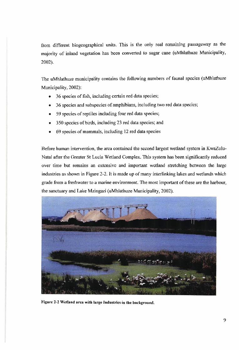
Before human intervention, the area contained the second largest wetland system in KwaZulu­

Natal after the Greater 8t Lucia Wetland Complex. This system has been significantly reduced

over time but remains an extensive and important wetland stretching between the large

industries as shown in Figure 2-2. It is made up of many interlinking lakes and wetlands which

grade from a freshwater to a marine environment. The most important ofthese are the harbour,

the sanctuary and Lake Mzingazi (uMhlathuze Municipality, 2002).

Figure 2-2 Wetland area with large Industries in the background.

9

Thesewetlands perform many fundamental ecological functions including; water purification,

water release during dry periods and animal breeding grounds (uMhlathuze Municipality,

2002). They also form the habitat of many species of aquatic avifauna, zooplankton,

ichthyofauna, macrocrustacea, benthic and other aquatic invertebrates (Cyrus, 2001).

Richards Bay is the largest town in the uMhlathuze Municipality and contains a substantial

industrial sector. This industrial sector has a widely dispersed arrangement with many of the

large extractive industries sparsely distributed within extensive areas of natural vegetation.

Although much of the area is zoned as industrial, large tracts are still covered by modified

natural vegetation as illustrated in Figure 2-3. These areas allow for many of the natural

ecosystem processes to continue to function.

Figure 2-3 Grassland area situated between large industrial areas in Richards Bay

The town of Richards Bay has a formal Metropolitan Open Space System (MOSS) that

incorporates public open spaces, formal play lots, sports and recreation facilities, community

centres, wide landscaped public streets with pedestrian walkways, and unspoilt natural areas

(uMhlatuze IDP, 2002). There are ten broad planning principles on which the MOSS is based.

They are; the systems hierarchical diversity, linkages, visibility and accessibility, natural

features and ecologically sensitive areas, landscaping, elimination of vacant/waste land and

the integration of streets and open spaces. These principles aid in the successful

implementation of the system (uMhlathuze Municipality, 2002).

10

2.3. History of the uMhlathuze Municipality

The first substantial human settlement in the area was in 1906 when Zululand Fisheries was

established at Richards Bay. Shortly after this in 1907, the first wagon track to the area was

built from Empangeni, allowing Empangeni to develop into a small village.

Empangeni grew slowly becoming an agricultural centre serving the farmers in the area, while

Richards Bay remained a small fishing village until the late 1960s when the South African

Railways and Harbours Administration decided it was time to build a new harbour on the

eastern coast that could accommodate large vessels. This development was part of an overall

National Development Plan and the harbour was to be linked to the main inland development

areas with a railway (Department of Planning, 1972). It was acknowledged at the time that this

development would lead to the growth of a large urban area containing industrial, commercial

and residential components.

A Richards Bay town board was established in 1971 to cover an area of 310 km2. The Board

had freedom to plan the new city around certain fixed features such as the harbour, aluminium

smelter, electricity substation, petro-chemical complex, railway marshalling yard and railway

lines whose locations were previously determined. The natural beauty of the area, recreational

potential of the bay and freshwater lakes were considered important assets and thus

incorporated as valuable resources in the planning (Department of Planning, 1972). The town

quickly grew into the largest and most important urban area in the uMhlathuze Municipality.

A large number of parties participated in the overall planning of development in the area

including authorities responsible for the future of the harbour, the railways, national roads and

electric power supply, as well as engineering services such as the road network, water supply,

storm water canals and drains, and sewerage and industrial pipelines (Department of Planning,

1972). This wide range of actors often meant conflicting desires and frequent adjustments to

plans.

11

Under the Apartheid regime the town of Richards Bay and the surrounding land was situated

in an area designated as a White population area and the land to the north and south was

designated as Homelands. The close proximity to Homelands influenced the citing of the

harbour, as there was at the time an industrial decentralisation policy that emphasised

development of industrial areas on the borders of Homelands. Also, particular attention in the

planning of the town was paid to large numbers of daily commuters coming into the industrial

areas from the surrounding Homelands (Department of Planning, 1972).

Since the inception of the harbour at Richards Bay, a national planning policy has stimulated

rapid industrial development in the area in support of the harbour and associated infrastructure

(uMhlathuze Municipality, 2002), and subsequently many large extractive industries have

been established owing to this infrastructure.

2.4. Development Strategies and Government Policies

Richards Bay is based on an industrial foundation with large extractive industries supporting

an affluent society in the formal sector. On the other hand, it also contains a very large

element of what Hall (2004) describes as a city coping with informal hypergrowth. A category

into which many cities in sub-Saharan Africa fall and are characterised by rapid population

growth from migration and natural increase and supporting economies heavily dependant on

the informal sector. Such cities contain extensive informal housing areas, widespread poverty

and environmental and health problems. Richards Bay contains both the formal and informal

sectors mixing together to give the prevalent trajectories of growth.

During the Apartheid era, Richards Bay experienced rapid industrial development as a

consequence of planning policies designed to stimulate industrial development in support of

the harbour and the towns close proximity to Homelands (uMhlathuze Municipality, 2002).

One such policy was the Decentralisation Policy, which was aimed at shifting investment in

the manufacturing industries away from the metropolitan areas and into designated growth

areas situated near or within the former Homelands to provide a rural-urban economic balance

(Kihato, 1999; Crush & Rogerson, 2001).

12

In 1996 the Spatial Development Initiative (SDI) programme was introduced as a support

pillar of South Africa's Growth, Employment and Redistribution (GEAR) macro economic

policy (Crush & Rogerson, 2001). The uMhlathuze municipality was designated an important

node of this programme, which was aimed at fostering sustainable industrial development in

areas where poverty and unemployment were at their highest and where economic potential

existed.

The SDI was set out to encourage economic growth and spatial redistribution (Hall, 2000).

Some of the main objectives include increasing foreign exchange and earning, substantial job

creation, restructuring the Apartheid economy, public-private partnerships, better utilization of

existing infrastructure and resources and broadening the ownership base of the economy. The

Richards Bay SDI includes 15 industrial projects that have been established since 1996 and

brought in new investment totalling just under 700 million Rand and 1039 new jobs. A further

19 potential projects are under consideration and six Small and Medium Enterprises (SMEs)

have been initiated (KZN DEDT, 2002).

The implementation of the SDI structure in Richards Bay has been criticised for reflecting,

rather than challenging the existing regional institutional structure, and has simply resulted in

a policy that may strengthen the existing and problematic development course (Hall, 2000).

Hall (2000) further notes that regional policies are frequently simply reflections of national

government strategies interpreted through the regional planners objectives, meaning that

development may simply continue in the same mode, without fulfilling all the objectives of

the SDI.

Richards Bay has clearly demarcated urban zones (Figure 2-4) and steers development through

a systematic Structure Plan framework that is related to long-term port expansion plans and a

predicted population of over one million people by 2030 (Hall, 2000). The framework has

allocated 1200 hectares of industrial estate for general industries and has stipulated five basic

nodes of industrial development in Richards Bay, they are:

• Alton and Alton North industrial areas;

13

• AlusafBayside Smelter;

• Mondi Kraft paper mill;

• AlusafHillside, Indian Ocean Fertiliser, CTC, Ben and Silvacel; and

• The coal terminal and harbour

"A

1~ 3 6'--------'-,----;;-;-;~~I:7::-:-:----------',

Kilometers

Figure 2-4 Map of the broad land use zones in Richards Bay

Land Uses

_ "'.lriculture

~Harbour

~ Open space and environmental

~ Urban commercial

_ Urban residential

c::::::::J Undertermined or special zones

_wale,Body

_ Urban i1duslrial

It must also be noted that, since Richards Bay developed around a few large industries, the

local economy is subject to boom-bust cycles associated with the construction of mega­

projects (Han, 2000).

2.5. Summary

This chapter has described the study site, including the location, the natural environment, the

history and relevant development strategies and government policies that have impacted on the

land cover changes in the area.

14

The uMhlathuze Municipality section gives basic information and provides a location map

showing the spatial distribution of the urban areas. The natural environment section describes

the vegetation and natural land covers, as well as the wetland system and faunal species

resident in the area. The MOSS system is also explained. The section on the history of the

uMhlathuze Municipality provides an account of the development of the area since the

establishment of the first two villages. The section on development strategies and government

policies gives a brief report on the various strategies and policies that have guided

development in the uMhlathuze Municipality such as the Decentralisation Policy and SDI.

15

CHAPTER 3. LITERATURE REVIEW

3.l.Ecological Urban Dynamics and Environmental Considerations

3.1.1. Urban Expansion and Population Growth

The United Nations Population Division (UNPD) (2002) estimate that the vast majority of the

population growth expected over the next 30 years will take place in urban areas; that half the

world population will live in urban areas by 2007 and that the vast majority of the population

increase between the years 2000 and 2030 will be absorbed by the urban areas of less

developed countries. Since most of the world's population resides in urban areas, it is in these

areas that economic, social and environmental processes will primarily affect human societies.

Urban areas have to maintain an equilibrium balance between economic activities, population

growth, and pollution and waste so that the urban system and its dynamic processes can evolve

in harmony with minimal impacts on the environment (Barredo et al., 2004).

In developing countries, urban growth often takes place for two main reasons, firstly, in

response to economic growth in the cities and secondly as a consequence of migration taking

place due to a lack of opportunity in rural areas (Wahba, 1996). The influx oflarge numbers of

people unable to generate revenue places immense strain on the planning and management of

urban areas. The high degree of land modification completely transforms the natural landscape

and forms new habitats and ecosystems, vastly different from the original habitats.

Informal settlements develop in areas without services or formal planning. These settlements

are frequently on unsuitable land, such as along rivers' and often grow quickly. Planners in

Developing countries usually do not have the financial means to adequately provide for such

settlements, leaving them to develop with minimal government guidance Campbell (1983).

Campbell (1983) notes that this type of uncoordinated development can lead to bad land use

patterns and conditions that are environmentally, socially and economically unfavourable.

16

The impacts of disturbance on the land, formation of urban heat islands and modifications in

nutrient dynamics such as an increase in chronic nitrogen inputs changes the local climate

preventing re-habitation of the original species. (Zipperer et al., 2000). Policy makers are

being forced to put environmental concerns high on the agenda as the destructive nature of

urbanisation is being realised. Consequently, Braissoulis (2001) notes that land use change is

increasingly becoming the subject of policy disciplines due to its strong relation with

environmental problems and climate change.

The densely concentrated human habitation in urban areas is maintained by the import of

materials and energy from external areas. This external dependence means that the human

system is not restricted by the constraints of the local ecosystems but extends the ecological

footprint of human influence beyond the boundaries of the city. However, with such an inflow

of materials and energy into the city, the city becomes a producer of other materials such as

finished goods and wastes (Luck et aI., 2001).

Sustainability of a city has come to the forefront of planners' agendas in recent years. The

main emphasis of sustainability is that every citizen present or future has a decent quality of

life (Laurini, 2001). Laurini (2001) points out the five main components of a sustainable city

model:

• The human economy: human activities in urban space;

• The city metabolism: material flows within and through urban space;

• Integrity of ecological life support system;

• Quality of human life: level of human needs satisfaction; and

• Vitality of ecological systems: status of species

These five aspects all need consideration and essentially need to be achieved simultaneously

to improve the sustainability of cities.

17

3.1.2. Urban Ecosystems

The spatial patterns of urban areas have received much attention from geographers and social

scientists (Harris, 1998) but there has been little work done on the ecology of these areas (Wu

et al., 2003). Urban ecological systems play a number of important roles such as; the

reduction of pollution, seed dispersal, air filtration, microclimate regulation, noise reduction,

rainwater drainage and sewerage treatment (Elmqvist et al., 2004). These systems are

characterised by complex interaction between humans and the natural environment at a variety

of spatial and temporal scales (Luck et aI., 2001).

Elmqvist et al. (2004) note that one of the key challenges is sustaining the capacity of

ecosystems to generate the services they deliver in growing urban areas. Planners and policy

makers need to understand how proposed land use changes will affect the ecological

components so as to produce strategies to preserve ecosystem capacity. Zipperer et al. (2000)

suggest that to understand and preserve the dynamics of urban ecosystems one needs to

incorporate the classic ecosystem approach and a patch dynamic approach. The ecosystem

approach concentrates on the magnitude and control of the fluxes of energy, matter and

species, while the patch dynamic approach concentrates on the spatial heterogeneity within

landscapes and how such heterogeneity affects energy flows, matter and species. Zipperer et

al. (2000) further note that an ecological approach to land use planning is essential to maintain

the long-term sustainability of ecosystem benefits, services and resources. In a similar fashion,

to account for human impacts on the urban landscape, the ecosystem concept needs to

incorporate humans as a component.

Zipperer et al. (2000) assembled a list of the key ecological principals needing attention in

urban land use change decision-making:

• Content refers to the structural and functional attributes of a patch where structure is

the physical arrangement of the ecological, physical and social components, and

function refers to the way the components interact;

18

• Context refers to the patch's location relative to the rest ofthe landscape as well as the

adjacent and nearby land units that are in direct contact or linked to a patch by active

interactions;

• Connectivity refers to how spatially or functionally continuous a patch, corridor,

network or matrix of concern is;

• Dynamics refers to how a patch or patch mosaic changes structurally and functionally

through time;

• Heterogeneity refers to the spatial and temporal distribution of patches across a

landscape. Heterogeneity creates the barriers or pathways to the flow of energy, matter,

species and information; and

• Hierarchy refers to a system of discrete functional units that are linked but operate at

two or more scales. Proper coupling of spatial and temporal hierarchies provides a key

to simplifying and understanding the complexity of urban landscapes.

Urban landscapes have great spatial heterogeneity at multiple scales made up of a mosaic of

biological and physical patches (Zipperer et aI., 2000). Modification of landforms, drainage

networks, extensive infrastructure and the introduction of exotic species all contribute to this

heterogeneity. Ecological processes operate at these various scales and thus any strategy to

conserve such processes and elements needs to encompass such a diversity of scales (Noss,

1991).

The arrangement of landscape elements such as parks, urban blocks, vegetation patches, golf

courses and agricultural fields influence many ecosystem processes such as water discharge

characteristics, primary production and nutrient cycling (Wu et al., 2003). These impacts need

to be understood to determine how development can proceed in a manner that has the least

possible impact on such processes. Wu & Qi (2000) suggest that spatial pattern analysis is an

important way of quantifying the changes to the landscape structure and relating landscape

pattern to ecological processes.

19

3.1.3. Urban Open Space

Urban open spaces are areas of either natural or modified vegetation such as parks, sports and

recreation facilities, community centres, wide landscaped public streets with pedestrian

walkways, and unspoilt natural areas. The central goal of urban open spaces is to manage and

maintain ecological processes at a regional scale (Flores et aI., 1998). They also provide a

variety of other benefits to cities such as the delivery of ecosystem services, areas for

recreation, places for tranquillity, educational value and the intrinsic values of nature.

Urban growth places barriers to species dispersion, isolating populations and rendering them

more vulnerable to extinction, due to reduced access to resources, genetic deterioration and

increased susceptibility to catastrophes (Noss, 1991; Leao et aI., 2004). Habitat fragmentation

is considered by many biologists to be the single greatest threat to biological diversity (Noss,

1991). Habitat sizes are important for the preservation of viable populations of certain species.

If areas of natural vegetation are situated strategically throughout the urban areas they can

provide landscape linkages and habitat corridors between large habitat patches. These linkages

reduce the impacts of fragmentation so prevalent in urban areas by allowing for species

migration.

Habitat connectivity has been found to be vital in the ability of urban green areas to support

biodiversity over long periods of time (Elmqvist et aI., 2004). A loss of diversity in an

ecosystem can lead to a loss of guilds, ecological services and long-term productivity, and

increases the vulnerability of the system to pest and invasive alien species (Wilson, 1994;

Begon et al., 1996). Greenways are corridors of open space connecting parks and natural

areas. Such areas may comprise a riverfront, a pathway, a stream valley or suchlike and play

important ecological roles as connectors of habitat islands (Hay, 1991).

Elmqvist et al. (2004) note that recreation is among the most important services provided by

urban open spaces. Open areas for playing sports, walking or just places where people can go

to find peace and quiet are all important aspects that people living in urban areas value. Also,

urban open spaces provide communication points between urban residents and nature and for

20

various social groups; the elderly, teenagers and children and thus they contribute to cultural

diversity and social cohesion in urban areas (Elmqvist et al., 2004).

Chapter 2 of the South African Constitution states that everyone has the right "to have the

environment protected through reasonable legislative and other measures that promote

conservation and secure ecologically sustainable development and the use of natural resources,

while promoting justifiable economic and social development". Likewise, chapter 10 of

Agenda 21 states that an integrated approach to the planning and management of land

resources requires the various levels of governments to review and develop policies to support

the best possible use of land and the sustainable management of land resources (United

Nations, 2004). These documents provide an official need to preserve natural areas in cities

and are partly achieved by Metropolitan Open Space Systems (MOSS), a strategy currently in

place at Richards Bay.

3.2.The Role of GIS and Remote Sensing in Land Use and Land Cover

Change

Land use and land cover studies have undergone large changes in both the planning and

technical contexts over the last six decades. In the 1940s and 1950s planning was based on

detailed land use maps produced at great expense. Since then the discipline has undergone a

series of technical developments. However, it was not until aerial photography and remote

sensing that substantial improvements came about (Kivel, 1991). At the same time manual

analysis and drafting gave way to digital mapping, computerised land management systems

and geographical information systems (GIS).

Prior to the 1980s, collection and compilation of data and publication of printed maps was

costly and time consuming (Borrough, 1986) and prevented many remote areas from being

mapped. Developments in both computers and GIS have increased the user-friendly nature of

model planning systems and allowed researchers to tackle problems previously considered

analytically impossible (Wilson, 1998 cited in Berling-Wolff & Wu, 2004). The scope of

opportunity is constantly increasing as the technical tools are developed.

21

3.2.1. The Benefits and Limitations of GIS

Biby and Shepard (1999) noted that the representation and analysis of land cover has been a

primary application of GIS since the technology was introduced in the early 1970s. GIS has

the ability to capture, convert, edit, update and manage data as well as several spatial analysis

functions and the ability to create high quality cartographic outputs (Chou, 1996). GIS tools

provide a method to quantify and measure the extent and spatial changes in land covers and

moreover can link these patterns to other spatially referenced dataset to provide information

on determinants of change and related factors.

A central function of GIS is the transformation of spatial data to information in a form that one

can use to aid in decision-making. Through functions such as spatial and database

manipulations one can transform and manipulate geographic data to add value to it and reveal

patterns (Longley et al., 2001). Although such analysis was possible before the advent of GIS,

the high functionality and speed of current software packages has brought these capabilities to

a far wider range of users.

The capabilities of GIS rely on both the availability and accuracy of the input data. A GIS is

designed for the purpose of processing spatial data so any errors or inconsistencies in the input

data will produce the same inconsistencies in the output, often compounded depending on the

processes carried out. The availability of good quality input data is accordingly critical to the

production of meaningful outputs. The development of remote sensing technology has

substantially aided in the provision of good quality data and has thus advanced the field of

GIS. It must be noted that the development of GIS and remote sensing capabilities has

increased the requirement for statistical measures to determine the accuracy of output data

(Congalton & Green, 1993).

22

3.2.2. The Benefits and Limitations of Remote Sensing

The term remote sensing can be defined as "the acquisition and recording of information about

an object without being in direct contact with that object" (Gibson, 2000: 76), and includes

both aerial photography and airborne satellite imagery. Aerial photography provides data in a

simple image format while satellite scanners record data in a number of light spectrum bands.

Such scanners allow the acquisition of data from wavelengths beyond the spectrum of visible

light, including the thermal infrared and microwave ranges (Gibson, 2000).

Different features on the ground surface have different reflectance values indicated by tonal

and textural differences in the remotely sensed imagery (Gibson, 2000). Lower reflectance

values are indicated by darker tones.(Land cover classes can be determined by grouping areas

with similar tones and textures. Each pixel in the image is assigned a digital number relating to

its reflectance value and only this spectral information given by the image is utilised. The

lower the reflectance value the lower the digital number. This digital nature of the data

medium lends itself well to digital analysis.

Weng (2002) notes that several previous studies of land use and land cover change (Muller &

Middleton, 1994; Brown et al., 2000; Hsu & Cheng, 2000) have utilised existing maps, aerial

photography or samples from field surveys in which data uncertainty is relatively high.

Satellite imagery creates an opportunity to improve this analysis. Weng (2002) further notes

that an operational procedure needs to be developed to effectively integrate the techniques of

satellite remote sensing and GIS with various modelling procedures to improve analysis of

land use and land cover change.

Some of the difficulties associated with the use of satellite remote sensing for change detection

include an absence of prior information about the shapes of changed areas, a lack of reference

background data, differences in light and atmospheric conditions, sensor calibration

difficulties, ground moisture and registration noise (Bruzzone & Cossu, 2002). One of the

dominant problems with classifying urban areas is the range of spectral responses stemming

from the heterogeneity of urban areas (Foody & Curran, 1994). Roofs, roads, concrete, trees,

and many other urban features present a range of spectral reflectance values both higher and

23

lower than other land cover classes, making it difficult to classify as a single class.

Classification approaches such as object-oriented classification take the form, textures and

spectral information into account and thus can improve the accuracy of the results (Omc et aI.,

2004).

3.2.3. Landsat Satellite Imagery

The National Aeronautics and Space Administration (NASA) with co-operation from the

United States Department of Interior launched the Landsat program of satellite in 1972. The

program had an 'open skies' principle meaning that there was non-discriminatory access to

data collected from the satellites anywhere in the world (Liellesand & Kiefer, 1994). There

was a total of seven satellites in the series, namely Landsat-l through Landsat-7. Landsat-l, -2

and -3 were very alike in operation as were Landsat-4 and -5. Landsat-6 experiencd a launch

failure and Landsat-7 was unique in operation as it contains an improved scanning radiometer.

Imagery from the Landsat-5 and Landsat-7 series was used in this study so only these two

satellites will be described in more detail.

Landsat-5 was launched on 1 March 1984 (Lillesand & Kiefer, 1994). It uses a Thematic

Mapper (TM) sensor which contains seven spectral bands with eight-bit radiometric resolution

and a 28.5 m spatial resolution for all bands except the thermal (band 6), which has a spatial

resolution of 120 m. The wavelengths of the spectral bands are produced in Table 3-1. This

satellite has a 16-day return period.

Table 3-1 Landsat-5 band wavelengths

Band Wavelength (microns)1, Blue 0.45 to 0.52/-lm

2, Green 0.52 to 0.60/-lm3, Red 0.63 to 0.69/-lm4, NIR 0.76 to 0.90/-lm5, NIR 1.55 to 1.75/-lm6, NIR 10.40 to 12.50/-lm7, NIR 2.08 to 2.35/-lm

(Developedfrom Lillesand & Kiefer, 1994)

24

Landsat-7 was launched in 1999. It uses an Enhanced Thematic Mapper Plus (ETM+) sensor

with a 15 m spatial resolution in the panchromatic band, a 30 m spatial resolution in the multi­

spectral bands, two radiometric sensitivity ranges and a 60 m spatial resolution thermal­

infrared band. It has a 5% radiometric calibration with full aperture. Landsat-7 also has a 16­

day return period. Table 3-2 provides the characteristics of the spectral bands. In May 2003

Landsat-7 experienced a fault with the Scan Line Corrector resulting in gaps in the processed

product.

Table 3-2 Landsat-7 Characteristics

Band Number Wavelength (microns)1 0045 to 0.52 I!m2 0.52 to 0.60 I!m3 0.63 to 0.69 I!m4 0.76 to 0.90 I!m5 1.55 to 1.75 I!m6 lOA to 12.5 I!m7 2.08 to 2.35 I!m

Panchromatic (8) 0.50 to 0.90 I!m(Taken from ERDAS, Inc, 1997)

Resolution (m)3030303030603015

The seven recorded bands, representing the different wavelengths, .allow a composite image to

be produced representing either true colour (blue, green, red) or a variety of false colour

composites allowing the user superior visual interpretation. It must be noted that certain bands

are often better suited to specific applications. Bands 4 and 5 are best for distinguishing urban

areas, roads, gravel pits and quarries, bands 6 and 7 are best for delineating water bodies,

bands 6 and 7 are best for geological studies and agricultural areas are best distinguished with

bands 5, 6 and 7 (Lillesand and Kiefer, 1994). Zha et al. (2003) found that a combination of

bands 2 (blue), 3 (green) and 4 (red) were most suitable for distinguishing between a range of

land covers including built up, woodland, farmland, barren lands and water. Weng (2002) also

found this combination most suitable for a similar application.

3.3.Determinants of Land Use and Land Cover Change

Land use and land cover changes take place primarily as a result of human actions in response

to needs and wants. A variety of other factors then influence the extent, pattern and rate of

25

such changes. In predicting future patterns of land use change, it is imperative that one

assesses the problem at the cause rather than simply addressing the symptoms. An

understanding of the factors causing changes will provide insight into the trajectories of

change.

Verburg et al. (2004) note that studies of land use change should conceptualise the interactions

among the driving forces of land use change, their mitigating procedures and human behaviour

and organisation. Human actions take place in response to the socio-cultural and physical

environment and are aimed at increasing their economic and socio-cultural well being

(Verburg et aI., in press). Land use patterns are a consequence of these human actions and

should not be viewed independently of the driving forces underlying the motivation for

production and consumption.

Urban growth plays a large part in changing land uses and land covers as land is quickly

transformed by developments. Urban growth stems from expansion of residential, industrial,

commercial and recreational areas (Verburg et al., 2004) and radically transforms the

landscape. The patterns and location of such changes are normally a result of spatial policies,

accessibility measures and neighbourhood interactions (Verburg et aI., 2004).Land use

decisions are often the product of both macro- and micro-level processes (Bergeron & Pender,

1999). The macro-level factors include land policies, markets, trade, aggregate population

growth and technology development, while the micro-level factors include the lands

biophysical characteristics, the human and economic endowment of the households and

community characteristics.

The three over-arching categories that need consideration in understanding determinants of

land use changes are environmental or biophysical, social and economic considerations. These

processes interact with each other leading to complex patterns of land use and land cover

change. One needs to understand the many factors within each group as well as the

relationships between the three groups to comprehend the prevalent land use changes

(Braissoulis, 2001). Verburg et al. (2004) discussed five dominant determinants of land use

change. These are spatial policies, economic factors, biophysical constraints and potentials,

26

social factors and spatial interactions. These five factors will be discussed in more detail

below.

3.3.1. Economic Factors

Economics is a vital determinant of land uses. The pattern of land use evolves primarily from

activities competing for sites through the process of supply and demand (Kivel, 1991).

Economists view the relation between land uses and location factors based on the assumption

that in equilibrium land is used for the activity that generates the highest potential profitability

(Verburg et al., 2004). However, there are many other relevant factors such as social change,

credit availability and inflation, which cause the urban land market to function imperfectly.

Furthermore, the land market is rarely a free market and often heavily constrained by local and

national governments. This results in the actual land use of a certain plot being somewhat

different to its potential land use in a planning context (Kivel, 1991).

It is also noted that the level of economic development of an area can have a bearing on land

use changes as it is often representative of the level of wealth of the population or society. The

level of wealth can influence access to resources available to a population and hence the

degree to which the landscape can be modified (Turner & Meyer, 1991). Similarly, levels of

wealth can shape the modes of land resource utilization.

3.3.2. Social Factors

Important social determinants of land uses include individuals' cultural values, norms,

preferences, and peoples' financial, temporal and transport means (Verburg et al., 2004). Site

characteristics can influence peoples' choices of residential areas. These include housing

prices, levels of services supplied, quality of landscapes and social composition of

neighbourhoods (Verburg et al., 2004).

Population growth has been found to be a principal factor driving land use changes (Turner

and Meyer, 1991; Verburg et al., 1999). Growth of a population increases the need for

27

residential, commercial, industrial and agricultural land. In highly populated areas competition

for land becomes a very contentious issue leading to several environmental and social

problems.

3.3.3. Spatial Interactions and Neighbourhood Characteristics

The land use of a particular area will normally be influenced by the land uses in adjacent

areas. Each development affects the conditions of neighbouring locations. Harbours will

generally be associated with bulk storage and industrial areas, and urban expansion will be

situated near existing urban areas. Certain land uses are attracted to each other while others

repel each other (Verburg et al., 2004).

Spatial relations often result from certain network interactions. Physical networks such as

roads, services and power supplies, and interaction networks such as related industries and

businesses, influence the choice of land use in an area (Verburg et al., 2004). In Third World

countries, housing can make a large claim on the land as inexpensive accommodation tends to

spread outwards rather than upwards (Robinson et al., 2004).

3.3.4. Biophysical Factors

The biophysical environment, whilst not a strong driver of land use change, is more important

in terms of land use allocation decisions (Verburg et al., in press). The natural environment

can provide constraints on the possible land uses. Soil formations and strength, geology and

drainage conditions can influence the suitability of a location for various land uses (Verburg et

al., 2004). Furthermore, physical factors, which although may not determine the amount of

land use change, are fundamental in determining the pattern (Hall et aI, 1995a).

3.3.5. Policy Factors

Both local and national policies can have a variety of influences, directly and indirectly on

land uses. It is important to understand how and why decision makers make their decisions, so

28

that the potential benefits can be exploited and the negative consequences minimised

(Bergeron & Pender, 1999).

Many policies relating to conservation, land tenure changes or areas designated for subsidised

developments, are manifested spatially (Verburg et aI., 2004). They can have a large influence

on the spatial pattern of land use changes. Lubowski et al. (2003) found that changes in

government policies in the United States of America had a large impact on land use changes.

They found that policies such as the Conservation Reserve Program (CRP) and government

payments to crop producers were significant factors impacting land use.

In South Africa several new policies have come into being since a majority government came

into power in 1994. The relevant land related policies and legislation include (Fourie, 2000):

• Restitution of land to those who were removed;

• Large scale formal housing development for low income groups;

• Restructuring the cities and towns;

• Upgrading and giving title to informal settlements; and

• Redistribution of land

Other relevant legislation includes; the Land Reform (Labour Tenants) Act No. 3 of 1996, the

Interim Protection of Informal Rights Act No. 31 of 1996, the Communal Property

Association Act No. 28 of 1996 and the Extension of Security of Tenure Act No. 62 of 1997.

South Africa has also established the Spatial Development Initiative (SDI) program, which is a

policy, aimed at fostering sustainable industrial development in areas where poverty and

unemployment are high and where economic potential exists. More detail of the SDI in

Richards Bay is provided in section 2.4.

3.3.6. Sugarcane Expansion

Sugarcane expansion is included in this section as the study site is an important sugarcane

growing area in South Africa and contains the largest sugar mill in the country. Sugarcane

29

growing is the leading agricultural practice in the uMhlathuze municipality and is vitally

important in terms of land use (uMhlathuze Municipality, 2002). It is the largest land use in

the municipality and has many impacts on both the economy and environment. Economic

trends within the South African Sugar Industry could trigger significant changes in land cover

in the uMhlathuze municipality.

The South African Sugar Industry contributes approximately five billion Rand annually to the

South African economy (Anon, 2003) It is a major contributor to rural economies and an

important provider of jobs in cane growing areas of South Africa (Maloa, 2001). The industry

provides jobs directly involved with sugar and also many upstream and downstream linkages

such as businesses supplying the industry (Maloa, 2001). In recent years much emphasis has

been placed on the development of small-scale Black growers, and the production of sugar on

communally held land has increased significantly since the late 1970s reaching 15% of South

Africa's total cane production in 2001 (Maloa, 2001). In 1992 the Small Grower Development

Trust (SGDT) was formed to improve the ability of small-scale Black growers to participate in

the market (Maloa, 2001).

The biophysical conditions present in the uMhlathuze municipality are excellent for sugarcane

(Low and Rebelo, 1998), and farmers obtain high sugarcane yields averaging 87.5 t/ha/annum

(Schulze et aI., 1999). In 1994, Tongaat-Hulett Sugar developed the largest private irrigation

scheme in South Africa in the uMhlathuze region. This scheme has had a large influence on

increasing sugarcane production in the area (Fortman, 2005 pers comm.).

3.4.Land Use and Land Cover Change Detection

3.4.1. The Importance of Change Analysis

Both human and physical forces are constantly modifying the landscape. Changes in

vegetation and landscape cover have ripple effects on many factors such as wildlife habitat,

fire conditions, regional planning and aesthetic and historical values. Changes in the landscape

30

are also determinants of the policy and management strategies of an area. Thus it is vital to

gain an understanding of the changes taking place.

Analysis of multi-temporal remote sensing images has been used for several applications

including monitoring land cover dynamics, damage mapping, risk assessment and urban

expansion assessment (Bruzzone & Cossu, 2002; Civco et aI., 2002; Weng 2002; Chen et aI.,

2003). The wide range of different applications (forest dynamics, ecological process, urban

grow, agricultural expansion, etc) leads to a variety of techniques designed for different

purposes (Bruzzone & Cossu, 2002). Such studies usually include the three main steps;

preprocessing, image comparison and analysis of the results.

3.4.2. Data Preprocessing

Preprocessing of remotely sensed imagery refers to the correction for geometric distortions,

radiometric deficiencies and atmospheric deficiencies, and the removal of data errors and

flaws (Mather, 1989). These operations are carried out prior to the analysis of the imagery.

The remote nature of the sensors allows an array of atmospheric conditions to cause

distortions and deficiencies in the signals received by the sensors. Similarly, the signals can be

hindered by the effects of interactions between both incoming and outgoing electromagnetic

radiation and the elements of the atmosphere (Lillesand & Kiefer, 1994).

The basic corrections are carried out in the ground receiving stations of the satellites.

However, further specified corrections are carried out by the user. However, not all corrections

need to be carried out for all imagery and all purposes. The relevant techniques depend on the

application and quality of the imagery (Mather, 1989).

Studies of temporal change involve the analysis of multi-temporal images that must be

compared to one another. They thus require a degree of consistency between the reflectance

values and registration of the different images to ensure they are comparable in both the

spectral and spatial domains (Lu et aI., 2004). This presents the need for further refined

preprocessing such as co-registration and radiometric calibration. Co-registering the images

31

ensures that the coordinates of the pixels in all the images represent the same area on the

ground (Bruzzone & Cossu, 2002), whilst, radiometric calibration ensures that the grey levels

of the images represent the same reflectance values in all the images.

Further limitations in multi temporal analysis can stem from differences in sun angles, soil

moisture, plant phenological state and sensor calibration (Jensen, 2000; Singh, 1989). These

factors can compromise the accuracy of simultaneous image analysis. Furthermore, spectral

and spatial resolutions of the different images are also important considerations when

attempting to compare different images (Lu et al., 2004).

3.4.3. Image Classification

Image classification is the process of categorizing the pixels of an image into a specific

number of individual classes based on set criteria (ERDAS, Inc, 1997). Categorisation is

primarily based on the spectral patterns and radiance measurements obtained in the various

bands of the individual pixels in an image (Lillesand & Kiefer, 1994).

Classification procedures employ a spectral pattern recognition procedure but can incorporate

the spatial relationships of certain pixels with those surrounding them. The process can select

the number of bands to be utilized in the process. Increasing the number of bands will increase

the likelihood of each land cover having a unique value (Gibson, 2000).

There are two broad categories of classification; supervised and unsupervised. Unsupervised

classification involves the use of algorithms to examine all the pixels in an image and

aggregates them into a set number of classes based on the natural groupings that are present in

the data (Jensen, 2000). The method is based on the premise that the values present within

each cover types should be similar and different from other classes. The classes resulting from

this method will only be distinct in a purely spectrally nature. The analyst needs to compare

the classes with reference data to determine what land cover each one represents (Lillesand &

Kiefer, 1994). Usually the user will specify the computer to use a large number of classes,

which are later, combined to more broad classes of interest.

32

Supervised classification involves three steps; (1) the training stage, (2) the classification

stage and (3) the output stage. During the training (or pilot) stage representative training areas

are identified and a numerical description of the spectral attributes of each particular land

cover type is developed. Thereafter the classification stage classifies each pixel in the image

into the land cover class to which it most closely resembles. The output stage involves the

production of an output image, tables of statistics and digital data files (Eastman, 2001).

One needs to take cognizance of the fact that supervised classification requires some prior

knowledge of the study site and the types of land covers that are present. Furthermore, the

analyst must stipulate, through training sites, the spectral profiles of the required classes

(Gibson, 2000). The process uses a decision rule to determine which class a pixel will be

allocated to. The three most common of these are the 'parallelepiped', the 'minimum distance

to means' and the 'maximum likelihood' decision rule.

The 'parallelepiped' decision rule is based on Boolean logic. Each signature has high and low

limits in every band as illustrated by the blocks in Figure 3-1. If a pixel's data values fall

between these limits for every band in a signature then the pixel is assigned to that signature

class. It is a quick method but generally provides poor results as the classes often overlap

giving areas of ambiguity (Eastman, 2001). The signature classes can have, what is referred to

as 'corners' allowing pixels to fall within a class when they are actually spectrally dissimilar

from the class mean (ERDAS, Inc, 1997).

N.~

J3 C"'.

____I'A'OtSoll

Figure 3-1 Diagrammatic illustration of the class allocation method of the 'parallelepiped' decision rule(taken from Eastman, 2001). .

33

The 'minimum distance to means' decision rule calculates the distance to each mean signature

class vector from each pixel. The candidate pixel is assigned to the class with the closest mean

as illustrated in Figure 3-2. This decision rule is one of the fasters and has been shown to

perform moderately well, however, problems do arise as it does not account for signature

variability (Eastman, 2001). In other words, outlying pixels of variable land covers such as

urban may be misclassified (ERDAS, Inc, 1997).

&3fWiAdata fife vahJes

Figure 3-2 Diagrammatic illustration of the class allocation method of the 'minimum distance to means'decision rule (taken from ERDAS, Inc, 1997).

The 'maximum likelihood' decision rule is the most complex of the three and allows for the

determination of the probability of each pixel belonging to a class where the probability is

greatest at the mean of the class and decreases away from the mean in an elliptical pattern

(Eastman, 2001) as depicted in Figure 3-3.

The algorithm initially calculates a considerable amount of information about the class

membership, including the mean and variance/covariance data of the signature (Eastman,

2001) From this information it assigns each pixel to the class that is considered statistically

most likely to have given rise to that pixel (Jensen, 2000).

34

() L-__---..,....-------------=2:55Band. 1

Figure 3-3 Diagrammatic illustration of the class allocation method of the 'maximum likelihood' decisionrule (taken from Eastman, 2001).

The 'maximum likelihood' decision rule considered the most accurate used in the ERDAS

IMAGINE system (ERDAS, Inc, 1997), as by using covariance matrices it accounts for a large

degree of variability in the signature classes. Nonetheless, this decision rule takes a longer

time to compute and it tends to over-classify signatures with large values in the covariance

matrix (ERDAS, Inc, 1997).

3.4.4. Classification Accuracy Assessment

Lillesand and Kiefer (1994) note that a classification is only complete when the accuracy has

been assessed. This is because a classified map is not a perfect representation of reality and

there will always be some errors. The only way to validate ones' results and determine the

extent of errors is to implement an accuracy assessment (Lu et al., 2004). Andersen et al.

(1976) set out a number of criteria that a remote sensing land cover classification should meet.

The first of these is that the minimum level of interpretation accuracy, in the identification of

land use and land cover categories from remote sensor data, should be at least 85%. For the

complete list of criteria see Andersen et aI., (1976).

There are two basic types of error in classified land cover maps; position error and thematic

error (Homing, 2004). Positional error occurs when the shape and size of a particular class is

correct but the placement on the map is incorrect. Thematic error occurs when a land cover is

misclassified and the quantity of cells in the classified image does not equal that of the

reference image (Pontius, 2000). These errors are commonly determined through the creation

35

of an error matrix, which compare the relationship between a set of known reference data and

the corresponding points within a classified image on a category-by-category basis (Lillesand

& Kiefer, 1994). Additional statistics such as Kappa coefficients can be used to further

determine the character of the errors (Pontius, 2000; Lu et al., 2004).

Error matrices allow the user to analyse the errors of omission (exclusion) and the errors of

commission (inclusion). An overall accuracy can be obtained, as well as producer's

accuracies which indicate how well the training set pixels of each cover type are classified,

and user's accuracies, which indicate the probability that a pixel classified to a certain

category actually corresponds to that category on the ground (Lillesand & Kiefer, 1994). The

producer's accuracy is determined by dividing the correctly classified pixels by the total

number sampled for each class. The user's accuracy is determined by dividing the correctly

classified pixels by the total number of sample pixels classified as that class.

Lu et al. (2004) noted that the following factors must be considered to properly generate an

error matrix on order to gain a fair assessment of the error:

• Ground truth data collection;

• Classification scheme;

• Sampling scheme;

• Spatial auto-correlation; and

• Sample size and sample unit

One needs to note that the results of the error matrix only indicate the accuracy of the

classification at the areas where the ground truth points were taken, and not the overall

accuracy of the entire classified image (Lillesand & Kiefer, 1994).

3.4.5. Change Detection Techniques

Change detection refers to the process of identifying differences in the state of an object or

feature by observing it at different time periods (Singh, 1989). Essentially, it is the

identification of temporal changes from a multi-temporal data set. Different land covers and

36

land uses result in different reflectance values, so areas where changes in a landscape have

occurred will result in changes in the radiance values of the pixels in that area. Thus by

overlaying one image on to another one can determine the pixels where the reflectance values

have changed from one date to the next.

There is a large number of change detection techniques (sometimes referred to as algorithms)

discussed in the literature (Singh, 1989; Mouat et al., 1993; Mas, 1999; Liu et al., 2004), and

research in this subject is an active topic (Lu et al., 2004). There is no single approach that is

optimal to every occasion and the choice of techniques relates to the specific application and

study site.

Change detection techniques can be divided into bi-temporal analysis and multi-temporal

analysis. Bi-temporal involves the analysis of images taken from two different dates and

multi-temporal involves the analysis of images from a number of dates in a temporal

trajectory. The majority of techniques have been developed for bitemporal studies, however,

many of them can be applied to multi-temporal analysis. Techniques can also be divided into

those classified independently and compared later and those simultaneously classified and

analysed (Singh, 1989).

Lu et al. (2004) grouped the techniques into seven categories as follows:

• Algebra (image differencing, image regression, image ratioing, vegetation index

differencing, change vector analysis (CVA) and background subtraction);

• Transformation (Principal Component Analysis (PCA), Gramm-Schmidt (GS) and

Chi-square transformations);

• Classification (Post-classification comparison, spectral-temporal combined analysis,

expectation-maximisation algorithms (EM) change detection and unsupervised change

detection);

• Advanced models (Li-Strahler reflectance model, spectral mixture models and

biophysical parameter estimation models);

• Geographical information system (GIS) approaches (includes integrated GIS and

remote sensing methods and pure GIS methods);

37

• Visual analysis (includes visual interpretation of multi-temporal image composite and

on screen digitising of changed areas); and

• Other approaches

Detail is only provided for the 'post classification comparison' technique as this was the

technique found most appropriate for the study.

3.4.6. Post Classification Comparison

This method, also known as 'delta classification', involves the comparison of independently

produced classified images (Singh, 1989). The different classes are coded and entered into a

matrix of change, from which the areas of change can be determined. The imagery from the

different dates is classified separately reducing the need to register the images to each other

accurately. It also minimises the problems from atmospheric and sensor differences between

the images. This technique can produce a complete matrix of change directions (Lu et aI.,

2004).

The accuracy of this method is largely dependant on that of the initial classifications as the

'difference image' accuracy is a result of the multiplication of the accuracies of the individual

classified images. For example if the two classified images have an accuracy of 80% each,

when they are integrated they will result in a 'difference image' accuracy of 64 per cent (0.80

x 0.80 = 0.64). Errors of mis-classification and mis-registration present in the classified

images are compounded in the integration process (Coppin et al., 2004). This technique

requires a large amount of time and expertise to create classification products (Lu et al., 2004).

38

3.5.Modelling Land Cover Change and Urban Landscapt_~

3.5.1. Introduction

The use of Geographic Information Systems (GIS) and remote sensing for land use and land

cover change analysis has been greatly increased by the development of models built on the

capabilities of GIS and remote sensing but with added functionality. Such models utilize the

capabilities of GIS and remote sensing in combination with statistical and mathematical

procedures to provide meaningful results for planners and decision makers.

A mathematical model is a purposeful abstraction designed to represent complex reality and

represents the various relationships between the different elements in a system as a series of

equations, in order to simulate the likely progression of the system (Masser, 1972). Only the

relevant features of a particular subject under consideration are incorporated in the model,

while unnecessary detail is not utilised. Models that describe changes in a system over time

are known as dynamic models. Simulation models (or predictive models) are a subcategory of

dynamic models designed to extrapolate predictions into the future. Models can also be

categorized as either deterministic or stochastic. Deterministic models produce a single value

result, while stochastic models incorporate some natural variation into the model to provide a

range of possible outcomes, i.e. the input values are not fixed and thus can predict different

outcome scenarios (Beltrami, 1987).

The general process of models involves fitting the model to a historical pattern of change and

then extending the same pattern to get likely future scenarios (Brown et al., 2000). The output

of such models can provide urban and regional planners with information needed to

understand land use and land cover systems and achieve their desired goals (Yang & Lo,

2003). Furthermore, these models are valuable tools for improving understanding and analysis

of the interactions between socio-economic processes, agricultural activities and natural

resource management (Brown et al., 2000).

39

3.5.2. The Development of Land Use and Land Cover Change (LUCC) and

Urban Landscape Models

Urban modelling began in the late 1950s when car ownership increased, causing traffic

problems and brought a realisation among planners of a need for scientific study (Berling­

Wolff & Wu, 2004). The introduction of computers increased processing capabilities and thus

the ability of planners to model cities. The first models in transportation studies were derived

from relating spatial interactions to Newton's law of gravitational force (Masser, 1972), and

sought to incorporate different activity systems according to their spatial distribution obtained

from interaction functions developed from Newton's gravitational theory.

Later, during the early 1960s the Lowry model was developed. This model was a combination

that linked together the production constrained gravity model and the attraction constrained

gravity model (Masser, 1972). Its primary purpose was to generate estimates of population

distribution that would work in and serve a particular sector and the transportation networks

pertaining there to. However, the early models based on gravity theory lacked the underlying

economic and behavioural theory required to accurately portray the urban dynamics (Berling­

Wolff & Wu, 2004).

Following this, efforts to simulate urban markets led to the development of models derived

from linear programming techniques. These models incorporated economic theory of land use,

the best known of these was possibly the Herbert-Stevens deterministic equilibrium model

(Berling-Wolff & Wu, 2004).

During the late 1960s, land use and transportation models became more integrated to form

more holistic models incorporating a wider range of determinants. For example the Integrated

Transportation and Land-Use Package (ITLUP) model. However, by the early 1970s there was

widespread realisation that urban models were failing due to a number of fundamental flaws.

They lacked underlying theoretical bases, required vast amounts of data, were complicated and

too expensive (Berling-Wolff & Wu, 2004).

40

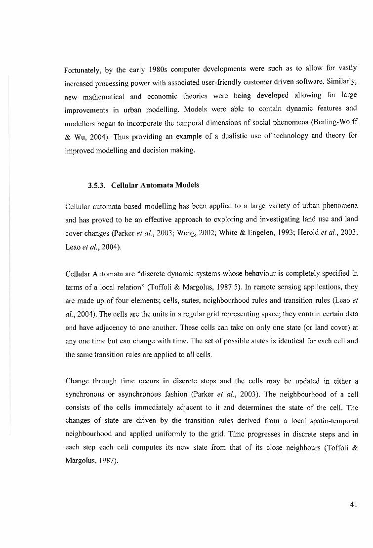
Fortunately, by the early 1980s computer developments were such as to allow for vastly

increased processing power with associated user-friendly customer driven software. Similarly,

new mathematical and economIC theories were being developed allowing for large

improvements in urban modelling. Models were able to contain dynamic features and

modellers began to incorporate the temporal dimensions of social phenomena (Berling-Wolff

& Wu, 2004). Thus providing an example of a dualistic use of technology and theory for

improved modelling and decision making.

3.5.3. Cellular Automata Models

Cellular automata based modelling has been applied to a large variety of urban phenomena

and has proved to be an effective approach to exploring and investigating land use and land

cover changes (parker et al., 2003; Weng, 2002; White & Engelen, 1993; Herold et al., 2003;

Leao et al., 2004).

Cellular Automata are "discrete dynamic systems whose behaviour is completely specified in

terms of a local relation" (Toffoli & Margolus, 1987:5). In remote sensing applications, they

are made up of four elements; cells, states, neighbourhood rules and transition rules (Leao et

al., 2004). The cells are the units in a regular grid representing space; they contain certain data

and have adjacency to one another. These cells can take on only one state (or land cover) at

anyone time but can change with time. The set of possible states is identical for each cell and

the same transition rules are applied to all cells.

Change through time occurs in discrete steps and the cells may be updated in either a

synchronous or asynchronous fashion (Parker et al., 2003). The neighbourhood of a cell

consists of the cells immediately adjacent to it and determines the state of the cell. The

changes of state are driven by the transition rules derived from a local spatio-temporal

neighbourhood and applied uniformly to the grid. Time progresses in discrete steps and in

each step each cell computes its new state from that of its close neighbours (Toffoli &

Margolus, 1987).

41

The transition rules determine the system dynamics by mapping the present state of a cell's

neighbourhood at time t, to an outcome state for that cell at time (t+ 1). The state of a cell is

generally representative of the land cover or land use of that cell but can also be representative

of land values, population densities and other such spatial classes (O'Sullivan & Torrens,

2001).

Since land use and land cover changes do not mutate in a predictable fashion such as cell

cultures on a microscope slide, but rather are a consequence of human agents such as

developers, firms, financiers, regulatory authorities, landlords and homebuyers (O'Sullivan &

Torrens, 2001), other transitions rules need to represent these factors, and are accordingly a

vital element in achieving a realistic model representing realistic system behaviour (Wu &

Webster, 2000). Transition rules provide a means of incorporating such external factors into

the progression of the model.

A cellular automaton is formally described as follows (Leao et al., 2004):

Q=<S,N,T>

Where Q = state of the system

S = set of all possible states of the system

N = Neighbourhood of all cells that provide input values for the transition function T

T = Transition function that defines the change in state of the cellular automaton.

Figure 3-4 illustrates how the cellular automata process progresses to model spatial changes in

a realistic growth manner.

42

Initial state {time t) Global stqte (time t+J)

D Vacant-cell

11 Non-vacant cell

• Cell corwertedfrom vacant into non-vacgnl at the lime step

Figure 3-4 Transition process of a generic cellular automaton (taken from Leao et al., 2004)

3.5.4. Markov Chain Models

Markov models are a form of cellular model and like cellular automata models, operate on a

lattice of congruent cells (Parker et aI., 2003). However, with Markov models the states of the

cells are probabilistically dependant on temporally delayed cell state values (Parker et aI.,

2003).

A basic Markov chain transition model can be expressed as follows (Brown et al., 2000):

Where nt is a vector of land area fractions in each land cover type at time t. nt+l is the vector of

land area fraction of the same types at time t+1. P is the matrix of the different land covers,

which illustrates the possibilities that the sites in state I at time t will change to state j at time

t+ I. This basic transition can be repeated several times using the updated matrix at each step

in the chain process.

When Cellular Automata and Markov chain models are combined, one can derive the benefits

of both modelling approaches to gain a more accurate modelling approach. When the cellular

automata component is added to a Markov model it allows the transition probabilities of a

43

certain pixel to be a function of the neighbouring pixels (Pontius & Malanson, 2005). Thus,

transitions can go through several states to give probabilistic land cover changes at many

temporal stages.

To apply a Markov chain model several assumptions are made. These include that the Markov

models are assumed to be a first order process, which means that the state at time t+1 is

dependant only on the state at time t and the transition probabilities (Cheng, 2000). In other

words, the antecedent conditioning before the study time period has no effect. Secondly, the

models are assumed to be stochastic as they are based on the transitions, which are simply

probabilities (Weng, 2002). Thirdly, the transition probabilities must remain stationary over

the time period (Baker, 1989), and lastly that land use change is not random over the time

period in the study (Muller & Middleton, 1994).

Cellular models are still simplistic and have difficulty representing urban dynamics and

incorporating human decision-making (Parker et al., 2003). Furthermore, since they operate

on discrete time steps while land use and land cover changes affect processes operating over

multiple timescales, they have trouble representing these processes (O'Sullivan & Torrens,

2001). Not withstanding these points cellular models have proved a valuable and accurate

means of simulating land cover change.

Brown et al. (2000) note that one of the primary limitations of Markov transition probability­

based models for land use and land cover change is the difficulty of assigning causes within

the model. The transition probabilities are derived purely from the transition stages of the

known land covers with no description of the processes taking place (Baker, 1989). This

limitation is of particular concern for study areas where changes are largely driven by social

and economic processes (Brown et aI., 2000). However, this problem can, to some extent, be

overcome by incorporating higher order effects, allowing for the influence of endogenous and

exogenous variables such as socio-economic factors or climate change and spatial effects

(Baker, 1989).

44

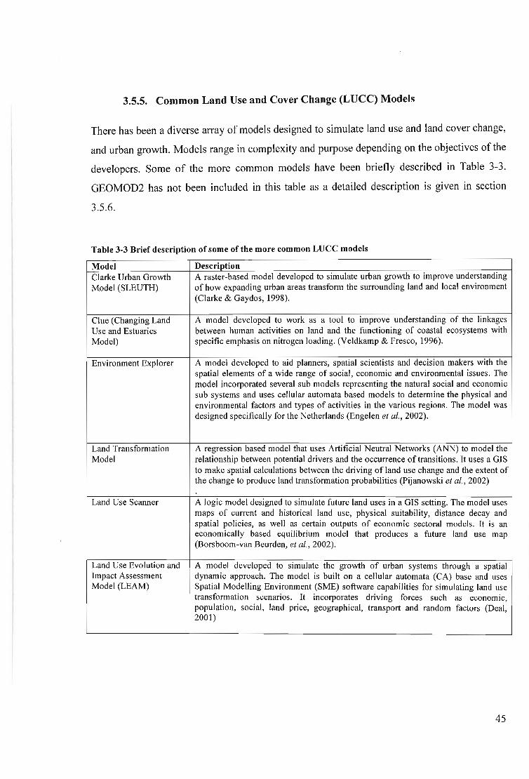
3.5.5. Common Land Use and Cover Change (LUCC) Models

There has been a diverse array of models designed to simulate land use and land cover change,

and urban growth. Models range in complexity and purpose depending on the objectives of the

developers. Some of the more common models have been briefly described in Table 3-3.

GEOMOD2 has not been included in this table as a detailed description is given in section

3.5.6.

Table 3-3 Brief description of some of the more common LUCC models

Model DescriptionClarke Urban Growth A raster-based model developed to simulate urban growth to improve understandingModel (SLEUTH) of how expanding urban areas transform the surrounding land and local environment

(Clarke & Gaydos, 1998).

Clue (Changing Land A model developed to work as a tool to improve understanding of the linkagesUse and Estuaries between human activities on land and the functioning of coastal ecosystems withModel) specific emphasis on nitrogen loading. (Veldkamp & Fresco, 1996).

Environment Explorer A model developed to aid planners, spatial scientists and decision makers with thespatial elements of a wide range of social, economic and environmental issues. Themodel incorporated several sub models representing the natural social and economicsub systems and uses cellular automata based models to determine the physical andenvironmental factors and types of activities in the various regions. The model wasdesigned specifically for the Netherlands (Engelen et al., 2002).

Land Transformation A regression based model that uses Artificial Neutral Networks (ANN) to model theModel relationship between potential drivers and the occurrence of transitions. It uses a GIS

to make spatial calculations between the driving of land use change and the extent ofthe change to produce land transformation probabilities (Pijanowski et al., 2002)

Land Use Scanner A logic model designed to simulate future land uses in a GIS setting. The model usesmaps of current and historical land use, physical suitability, distance decay andspatial policies, as well as certain outputs of economic sectoral models. It is aneconomically based equilibrium model that produces a future land use map(Borsboom-van Beurden, et al., 2002).

Land Use Evolution and A model developed to simulate the growth of urban systems through a spatialImpact Assessment dynamic approach. The model is built on a cellular automata (CA) base and usesModel (LEAM) Spatial Modelling Environment (SME) software capabilities for simulating land use

transformation scenarios. It incorporates driving forces such as economic,population, social, land price, geographical, transport and random factors (Deal,2001)

45

3.5.6. GEOMOD2

GEOMOD2 is a GIS based model that measures factors associated with land use change and

simulates changes in the land cover both forwards and backwards in time (Pontius et a1.,

2001). The model is primarily based on Markov Chain Analysis and Cellular Automata, which

allow it to predict the transition from one land cover state to another. The model simulates the

spatial patterns of land use change based on the patterns of biogeophysical attributes and

existing land uses derived from digital raster maps. (Hall et al., 1995a). These biogeophysical

attributes allow the model to determine how land is developed over space and time, and to

simulate how such patterns are likely to continue (Hall et a1., 1995a).

GEOMOD2 uses a statistical analysis of how people use land (Hall et a1., 1995b) to determine

the spatial patterns of change most likely to occur. It is an empirical adaptation of

GEOMOD I, which used data on elevation and slope through hypothesis deduction for the

purpose of simulating land cover change in tropical Asia (Hall et a1., 1995a). GEOMOD2 only

uses two land cover categories and predicts the change from one land cover to the other.

The predictive model uses three decision rules to select the locations of land to be converted

(Pontius et a1., 2001), as illustrated in Figure 3-5. The first decision rule is derived from the

nearest neighbour principal and ensures that in each time step the model limits the

development of a land cover to areas adjacent to the land cover. The second decision rule is

based on the biogeophysical attributes of the study area. This rule allows the model to predict

changes at locations that have attributes similar to that of the land cover to which an area can

change. This rule uses a suitability map created from several attribute maps such as elevation,

soil type, soil moisture, land use zones, proximity to transportation networks and precipitation.

The suitability map contains high values in areas where the biogeophysical attributes are most

suitable to expanding land cover, and low values in areas where the biogeophysical attributes

are least suitable for the expanding land cover. The model then simulates future changes in

areas that have the highest available suitability value (Pontius et a1., 2001). Each of the

attribute layers is weighted depending on the impact of that particular factor on the land cover

change.

46

The third decision rule involves sub-regional stratification. This decision rule is optional and

specifies the amount of land use change per time step in each of a number of sub-regions

within the study area (Pontius et aI., 2001). This rule permits the user more control over where

the changes may take place.

l;F,OMOD2

No. of pixelsestimated to

changeBiogeophysical

attributes

.Attribute layersweighted and

overlaid

Figure 3-5 Diagrammatic representation of GEOMOD2 land use and land cover change model (adapted

from Pontius et aL, 2001).

GEOMOD2 has dominantly been used to predict land development in tropical areas (Hall et

al., 1995a; Hall et al., 1995b; Pontius et al., 2001), but has also been used in Massachusetts,

USA (pontius et aI., 2004; Pontius & Malanson, 2005). Applications in tropical areas have

concentrated on patterns of deforestation and natural vegetation loss, and the resulting

impacts, while application in Massachusetts concentrated on changes from non-built to built

land. The model has been specifically designed to be robust enough to perform in various

study sites in many parts of the world (Pontius et al., 2001).

Various studies have found GEOMOD2 to provide very accurate results, usually between 80%

and 90% (Hall et al., 1995a; Hall et aI., 1995b; Pontius et al., 2001). The accuracy of the

model is mainly affected by time scale used, the number of land cover classes used and the

accuracy of the initial data (Hall et al., 1995b). The shorter the predictive time span and the

fewer the number of land use classes the more accurate the model (Hall et al., 1995b).

47

GEOMOD2 simulates the pattern and locations of land cover change and not the quantity,

which must be obtained from another source. Pontius et al. (2001) emphasize that it is a good

idea to merge GEOMOD2 with another model that predicts the quantity of land use change

over time.

3.5.7. Model Validation

Validation is an important part of Land Use and Land Cover Change (LUCC) modelling as it

provides a means to analyse the likely success of a model to a particular situation. Validation

allows the user to determine the truthfulness of the model in accordance with the problem

domain and how closely the outcome represents the real system behaviour (Parker et aI.,

2003). If models are not validated or have been poorly validated they can give the modeller a

misleading understanding of the models accuracy (Pontius et al., 2004). A model's usefulness

can only be measured by an objective evaluation of the design and performance (Gardner &

Urban, 2003) Assessment of the design involves a qualitative assessment of the model

structure while analysis of the performance involves a quantitative comparison of predictions

against independently gathered information (Gardner & Urban, 2003).

Model validation has been defined as "a demonstration that a model within its domain of

applicability possesses a satisfactory range of accuracy consistent with the intended

application of a model" (Rykiel, 1996:230). This is achieved by using the model to predict a

period of time for which there is a known set of reference data and then compare the model

results to known data.

In the remote sensing software package Idrisi Kilimanjaro (Clarke Labs, 2003) there is a

function called 'VALIDATE', which provides statistics for measuring the similarity between

two qualitative images, such as specified Kappa statistics, that enable one to distinguish

between errors of quantity and errors of location (Eastman, 2001). The Kappa statistics

include (Pontius, 2000; Eastman, 2001):

48

• Kappa for no information (Kno) - The proportion of pixels classified correctly relative

to the expected proportion classified correctly by a simulation with no ability to

specify accurately quantity or location;

• Kappa for location (Klocation) - The simulation's ability to specify location correctly;

• Kappa for quantity (Kquantity) - The systems ability to specify quantity correctly;

• Kappa standard (Kstandard) - A measure of a systems ability to attain perfect

classification;

• Value of Perfect Information of Location (VPIL); and

• Value of Perfect Information of Quantity (VPIQ)

This breakdown allows the user to analyze the success with which one can specify the location

of change and the quantity of change.

3.5.8. Recent Developments in Urban Modelling

Many modellers have modified the basic Cellular Automata (CA) model to improve accuracy

or to incorporate specific factors such as ecological systems or human behaviour (Deal, 2001;

Parker et aI., 2003). Most LUCC models, especially those developed for urban applications are

founded on relationships between location, density and urban evolution. Through the use of

fractal geometry and the laws of particle physics, modellers are able to link the growth process

to the geometry of the system. By combining the ideas of evolution, self-organisation and

fractal geometry with cellular automata it is possible to achieve high levels of spatial detail

and realism (White & Engelen, 1993). Modellers are continually developing new techniques to

improve the accuracy and application of models.

Parker et al. (2003) proposed the use of a multi-agent system model of land use/land cover

change (MAS/LUCC models) to complement existing modelling approaches and improve the

accuracy. Their models combined cellular modelling and multi-agent modelling into an

integrated system. The cellular component represents the landscape and transitions and the

agent-based component describes the decision-making architecture of the key actors in the

system and focuses on human actions (Parker et al., 2003). The model addresses the

49

limitations of equation-based models when representing dynamic processes and feedbacks.

They found that MAS/LUCC models offer important tools to assisting progress in

understanding the processes of land use and land cover change.

Herold et al. (2003) used spatial metrics in combination with SLEUTH urban growth model to

provide a time series of the development of Santa Barbara, California. The spatial metrics

were used to quantify the spatial and temporal characteristics of development in the area,

while the SLEUTH model was used to fill in the gaps in historical data and provide a forecast

of growth patterns for the year 2030.Leao et al. (2004) noted that CA-based models have been

chiefly developed for urban areas of the developed world. Since urban expansion occurs

through largely different processes in the developed and developing worlds, the applicability

of such models to the third world has been questioned. However, Barredo et al. (2004) used a

prototype cellular automata model to simulate urban growth in Lagos, Nigeria and found the

model to be highly effective and realistic. Similarly, Leao et al. (2004) applied a slightly

modified version of the Urban Growth Model (UGM) to Porto Alegre City in Brazil and also

found the model to be successful.

There are currently several developments in spatial modelling techniques for ecologically

based systems designed to improve approaches to incorporating ecological processes into

urban system modelling (Deal, 2001). These techniques utilize modern ecological theories

such as hierarchal patch theory, in conjunction with dynamic urban systems modelling (Deal,

2001; Wu et al., 2003).

In a similar study, Landis et al. (1998 cited in Berling-Wolff & Wu, 2004) developed the

California Urban and Biodiversity Analysis (CURBA) model, which included many features

for simulating the effects of different development and conservation policies on urban growth

patterns. Other related cellular models such as the Land Use Evolution and Impact Assessment

Model (LEAM) utilise a Spatial Decision Support System (SDSS) to evaluate the patterns of

human development (Deal, 2001). The LEAM nodel describes land use changes resulting from

the interactions of economic, ecological and social systems (Deal, 2001).

50

3.6.Summary

Firstly, this chapter described the environmental impacts of land use and land cover changes

and the importance of ecosystem processes and environmental sustainability in urban areas.

Secondly, the drivers and determinants that influence the rate, extent and patterns of land use

and land cover change were discussed. It is critical to have a clear understanding of the driving

forces to fully understand the patterns of change taking place over time.

Section 3.2 provided a description of the capabilities of GIS and remote sensing and the roles

these technologies play in land cover change analysis. Following this, the considerations and

processes of land cover change detection were discussed. Lastly, a detailed account was given

of LUCC models which build on the data and technology provided by both GIS and remote

sensing. A brief explanation was given of the underlying mathematical processes and

important considerations. Particular attention was given to one such model, GEOMOD2 as

this was the model used in the study.

51

CHAPTER 4. METHODS

4.1. Introduction

This chapter describes the data used and the methods undertaken during the study. The data

and the preprocessing of the data is described. The methods used for the image classification

and change detection procedures are explained, and an account is given of the procedures

followed during the predictive modelling section. Diagrams are used to provide a clear

demonstration of the processes carried out.

4.2. Data

4.2.1. Satellite Imagery

The primary data used in the study was a set of three satellite images representing the study

area at a frequency of five years. Images were choosen at five-year intervals representing the

years 1992, 1997 and 2002, and were obtained during the months of July, August and October

respectively. Five year intervals were chosen to provide an accurate trajectory of the changes

taking place. It was attempted to obtain imagery from dates in the same season to reduce

problems resulting from seasonal changes such as different sun angles and changes in plant

phenology (Singh, 1989).

Images from Landsat-5 TM and Landsat-7 ETM+ series were used due to their availability and

finer spectral resolution than other commonly used satellites such as SPOT, NOAA-AVHRR

and MODIS.

4.2.2. Data Preprocessing

Before any analysis took place the imagery was subjected to a preprocessing stage, which

included radiometric calibration and co-registration of the three images. For temporal

52

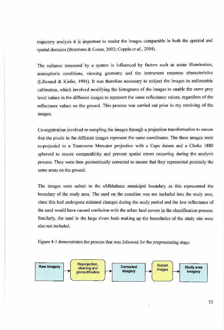
trajectory analysis it is important to render the images comparable in both the spectral and

spatial domains (Bruzzone & Cossu, 2002; Coppin et al., 2004).

The radiance measured by a system is influenced by factors such as scene illumination,

atmospheric conditions, viewing geometry and the instrument response characteristics

(Lillesand & Kiefer, 1994). It was therefore necessary to subject the images to radiometric

calibration, which involved modifying the histograms of the images to enable the same grey

level values in the different images to represent the same reflectance values, regardless of the

reflectance values on the ground. This process was carried out prior to my receiving of the

images.

Co-registration involved re-sampling the images through a projection transformation to ensure

that the pixels in the different images represent the same coordinates. The three images were

re-projected to a Transverse Mercator projection with a Cape datum and a Clarke 1880

spheroid to ensure comparability and prevent spatial errors occurring during the analysis

process. They were then geometrically corrected to ensure that they represented precisely the

same areas on the ground.

The images were subset to the uMhlathuze municipal boundary as this represented the

boundary of the study area. The sand on the coastline was not included into the study area,

since this had undergone minimal changes during the study period and the low reflectance of

the sand would have caused confusion with the urban land covers in the classification process.

Similarly, the sand in the large rivers beds making up the boundaries of the study site were

also not included.

Figure 4-1 demonstrates the process that was followed for the preprocessing stage.

Raw ImageryReprojection,

Corre~tedSubset StudY,area

~cleaning and

f----. imagery ~images

~georectification imagery

53

Figure 4-1 Flowchart of the steps undertaken during the preprocessing stage.

4.3.Change Detection

The change detection algorithm selected for this study was 'post classification comparison'

(Singh, 1989), which involves the comparison of independently produced classified images.

This method was chosen as the study utilised imagery from different Landsat satellite series

and the study site experienced great variation in rainfall during the study years. This algorithm

has proved favourable under such circumstances (Singh, 1989). Furthermore, by classifying

the images separately, one minimises the problem of radiometric calibration between the

different dates (Coppin et a!., 2004). However, this approach relies on the accuracy of the

initial image classifications as misclassifications in this stage are compounded when multiple

images are compared (Jensen, 2000). Emphasis was therefore placed on obtaining accurate

initial image classifications.

4.3.1. Image Classification

The images were viewed through a combination of bands 2 (green), 3 (red) and 4 (near

infrared) (Figure 4-2, Figure 4-3 and Figure 4-4) as these were found to be the most suitable in

other similar studies (Weng, 2002; Zha et a!., 2003), and gave the best visual distinction

between the land covers used in this study. The profiles in Figure 4-5 illustrate the spectral

differences of the broad land cover classes across the spectral bands. Although the variety is

greatest across the bands three, four and five, the classes were found to be best distinguished

using the above-mentioned band combination.

Polygons were drawn in areas representative of the different land covers to denote the training

sites from which the class signature would be developed. A total of 60 training sites were

selected for eleven land cover sub classes in each image. The large number of training sites

increased the accuracy of the spectral signatures for each sub class.

54

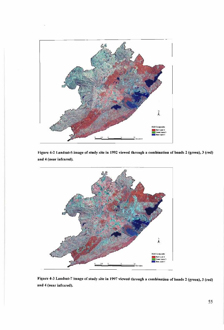
RGB CO'l1'o&ite

_Red:Layer4_Green: Layer 3_SlUe:Layer2

~,,!,!2§5=~~~~==...:ilOKilomEters

Figure 4-2 Landsat-5 image of study site in 1992 viewed through a combination of bands 2 (green), 3 (red)

and 4 (near infrared).

N

A

RGB COlllposke

_Red:la'fef4.Oreen:L.ayer3_SJue:Layer2

Figure 4-3 Landsat-7 image of study site in 1997 viewed through a combination of bands 2 (green), 3 (red)

and 4 (near infrared).

55

140 ~-------j

N

A

RGB Composite

_Red: Layer 4­_ Green; Layer 3

_Bll.le:Layer2

Figure 4-4 Landsat-7 image of study site in 2002 viewed through a combination of bands 2 (green), 3 (red)

and 4 (near infrared).

- ,Cut Cane

- .Cut forestry I120 +----- - - - ·Coal -------------,:io:-------

-Industrial Built-~ I100 -Commercial forestry

Q) +----- ~Grasslands i------------.L-~\------

.2 - - Natural Forest~ 80 +-----j -Residential Built-~ I

-)(Q) Sug- arcane II": 60 +-----j-VlBterSalt I '·'-IJ'J.'R- ~\'---_

III - - - •VlBter Fresh~ 40 +--~~~--------~~~~c;;#.ML-----~~---

o+-----.-----,---------.-------,----~---~---.-:~~

2 3 4Bands

5 6 7

Figure 4-5 Spectral profiles of the 11 broad land cover classes in the study area, taken from the 1992

image.

56

Classification was carried out in ERDAS Imagine 8.7 (Leica Geosystems, 2003) and achieved

through a 'supervised classification' process which divided the area into eleven initial land

cover classes based on the spectral properties of the user defined training sites. The training

sites for the different land cover classes were developed and verified with the aid of recent

land use maps, aerial photographs and visits to the study area. Class signatures were evaluated

using image alarms, spectral profiles, matrices and histograms (ERDAS, Inc, 1997).

The three satellite images were classified separately using consistent land cover classes

developed from the South African classification system (Thompson, 1996). Certain categories

of this system were combined together whilst other categories were modified to suit the

purpose of the study. The classification was based on this system to allow the results to be

viewed in the light of other studies as recommended by Jensen (2000).

Some of the initial eleven sub classes were combined to give a total of seven broad classes to

avoid complications arising from too many classes whilst still depicting the relevant

differences in land cover. The seven broad classes and descriptions of each are given in Table

4-1. The larger number of initial classes (eleven) was used as the land cover classes

'sugarcane' and 'forest and woodlands' contained patches with cover at different stages of

growth depending on the life stage of the crops.

Table 4-1 Description ofIand cover classes used in the study

Class DescriptionCommercial/industrial built Areas for the conduct of commerce and other mercantile business or includingup land major industrial or transport related infrastructure.

Residential built up land Areas where people reside on a permanent or near permanent basis. Includesboth formal and informal settlement areas, ranging from high to low buildingdensity.

Forest and woodlands All wooded areas with greater than 10% tree canopy cover. This categoryincludes natural forests, mangrove forests and commercial plantations.

Grasslands All areas of grassland with less than 10% tree and or shrub canopy cover andgreater than 1% total vegetation cover, dominated by grass-like, non-woody,rooted herbaceous plants.

57

Sugarcane Includes areas currently under sugarcane, fallow land and land being preparedfor planting. Sugarcane is, by far, the dominant cultivated crop in the area andcontained a relatively unique spectral signature.

Waterbodies Areas of (generally permanent) open water. This category includes natural andman-made waterbodies, which are either static or flowing and contain fresh,brackish or salt water conditions.

Mines and quarries Areas in which mining activity has occurred or is occurring. Includes both opencast mines and quarries, as well as surface infrastructure, mine dumps etc.,associated with underground mining activities.

The sub classes included; residential built up land, commercial/industrial built up land,

commercial forestry, cleared commercial forestry, sugarcane, cleared sugarcane, natural

forests, grasslands, fresh waterbodies, saline waterbodies, coal terminal and mining. Many of

these were then combined together after the classification process had been carried out, to give

the seven broad classes as indicated in Table 4-2.

Table 4-2 Broad classification classes with sub-classes

Broad Classes1 Commercial/industrial built-up land

2 Residential built-up land3 Forest and woodlands

4 Grasslands5 Sugarcane

6 Waterbodies

7 Mines and quarries

Sub ClassesCommercial/industrial built up landCoal terminalResidential built up landCommercialforestryCleared commercial forestryNatural forestsGrasslandsSugarcaneClearedsugarcaneFresh waterbodiesSaline waterbodiesMines and quarries

The training site locations for the different categories remained as spatially uniform as

possible across the different images, with only small alterations being made to the training site

polygons of the categories; cleared cane, cleared commercial forestry and grasslands, where

it was not possible to have uniform polygons. This uniformity ensured consistency in the

spectral signatures between the three different images and minimised apparent false changes in

land cover resulting from different signature selections for the same land cover categories.

58

The classification process used a 'maximum likelihood' decision rule, which is one of the

most accurate of the common decision rules (Eastman, 2001). This decision rule uses the mean

and variance/covariance data of the signatures to determine the likelihood that each pixel

belongs to a specific class. The probability of a pixel belonging to a class is highest at the

mean position of the class and decreases in an elliptical pattern away from the mean (Eastman,

2001).

The three classified images were filtered with a statistical filter comprising a 3x3 pixel

window size and the function set to median. This reduced the problem of individual

misclassified pixels within uniform land cover areas (Schneider & Pontius, 2001; Daryaei,

2003; De Kok et al., 2003).

The major rivers within the study site contained large riverbeds with stretches of open sand.

As with the rivers making up the boundary of the study site, the open sand was confused with

urban areas in the classification process, thus these rivers were digitized and automatically

classified as waterbodies reducing the problem ofmisclassification and increasing accuracy.

Figure 4-6 below provides a flow diagram of the steps undertaken during the Imageclassification process.

59

Carry out supervisedSubs(!t image to Development Evaluate classification

st~dyarea of training training site (Maximum likelihood)sites signatures

ClassifiedImages

Rivers (vector)

~ Statistical filter

Buffer rivers (3X3, median)

(80m)

1Convert to Rivers (raster) Reclassify to FiltefC!c;I

~ ImageSraster six classes

/

Final ClassifiedReclassify Automatically

to combine rivers classify river bedsImages and waterbodies as rivers (Boolean

operation)

Figure 4-6 Flow chart of the steps undertaken during the classification process.

4.3.2. Accuracy Assessment

An accuracy assessment was carried out to determine how accurately the classified images

represent the true land cover of the uMhlathuze municipality (Dai & Khorram, 1998; Guild et

al., 2004). Such an assessment provides a means for the user to determine the confidence that

one can gain from the classification results.

A lack of reference data for the years 1992 and 1997 rendered it impossible to carry out

accuracy assessments of all three images. Consequently this was only attempted for the 2002

image, which although was also somewhat out ofdate (accuracy assessment points recorded in

60

early 2005), was considered, from personal observations, comparable to the present land

covers in the uMhlathuze municipality. It was, however, essential that ground truth points

were taken only in areas where there was a strong indication that the land cover had not

changed since at least 2002. This lack of optimal reference data presented a limitation to the

study but adequate measures were taken to reduce the impacts. It must also be noted that the

study was as much about developing the techniques as it was about the accuracy of the [mal

products.

With the use of a Global Positioning System (GPS), a total of 48 ground truth points were

recorded in the uMhlathuze municipality where access was feasible (Figure 4-7). A larger

number of points would have increased confidence in the accuracy assessment. However, time

constraints prevented a larger number from being collected. At each point a true description of

the actual land cover was recorded and compared to the land covers at these points on the

classified image. Difficulty was experienced in attempting to obtain ground truth points for the

land covers waterbodies, commercial/industrial built-up land and mines and quarries, as

access to these areas was either restricted or problematic.

N

A

• Ground truth points

Figure 4-7 Location of the ground truth points used in the accuracy assessment.

61

An error matrix was subsequently produced to compare the relationship between the known

reference data (land cover recorded at the GPS points) and the corresponding pixels on the

2002 classified image on a category-by-category basis (Lillesand & Kiefer, 1994). From this,

the errors of omission (exclusion), errors of commission (inclusion), and an overall accuracy

were established.

4.3.3. Change Detection

Once the classification process was complete, the classified images were compared on a pixel­

by-pixel basis to determine the quantity, location and direction of land cover changes. Firstly,

all the pixels classified to each unique land cover class were summed to determine the changes

in quantity and proportion during the two time periods, 1992 to 1997 and 1997 to 2002.

Secondly, difference images were developed to establish the location of the changes and

determine how many pixels changed from one land cover to another.

This was achieved through a layer subtraction in Image Calculator of the Spatial Analyst

extension within ArcGIS 8.3 (ESRI, 2003) and gave unique values to all the possible class

changes that could have taken place, This resulted in the creation of a change map consisting

of pixel values ranging between 9 and 59, each number representing a different change from

one land cover to another. From these results, change matrices were constructed to

demonstrate the development of changes in the land cover classes.

4.4. Land Use and Land Cover Change Modelling

The final step of the analysis process involved the simulation of a predictive land cover image

for the year 2012. This was achieved through the use of a land cover change simulation model

named GEOMOD2, provided by Idrisi Kilimanjaro (Clarke Labs, 2003). The predicted image

was based on the changes taking place between the 1992 and 2002 images. The 1992 image

were chosen as this provided a ten year period and the model was set to predict changes over a

62

ten year period from 2002 to 2012. The years 1992 and 2002 also contained similar rainfall

condition allowing readily comparable classification results.

GEOMOD2 simulates change between only two land cover classes, and therefore the land

cover classes forest and woodlands, grasslands, cultivated lands, waterbodies, and mining and

quarries were reclassified to non-built-up and the land cover classes commercial/industrial

built-up land and residential built-up land were reclassified to built-up. A suitability image

was created to stipulate where transformations could take place and was incorporated, along

with other inputs, into the GEOMOD2 predictive change model.

It was assumed that the state in the year 2012 is dependant only on the state in the year 2002

and the transition probabilities, and that the history before the time period of the study has no

effect. Secondly, it is assumed that transition probabilities remain stationary and are not

random over the predicted time period between 2002 and 2012. These assumptions are

necessary for all Markov based land cover change models (Baker, 1989; Cheng, 2000).

4.4.1. Creation of the Suitability Image

A suitability image was created to influence the spatial increase of the built-up land cover

class. This image is used as a decision rule designed to guide the model to predict land cover

changes according to realistic system behaviour (Wu & Webster, 2000).

The suitability image was developed from criteria deemed important in determining the

appropriateness of a pixel to support the built-up land cover. It influences how, and in which

areas, the built-up land cover will increase. The choice of criteria was based on previous

studies (Hall et aI., 1995a; Deal, 2001; Parker et aI., 2003; Barredo et aI., 2004; Yang & Lo,

2003), the availability of data and the ability of the model itself. The criterion used was the

uMhlathuze municipality's demarcation of urban zones, and the constraints, or areas to be

excluded, included large waterbodies, areas within a proximity of 40 m to the centre of large

rivers and areas zoned as either wildlife sanctuaries or other protected areas.

63

The suitability image was created using Multi-Criteria Evaluation (MCE) in the IDRIS

software package, which incorporates the criteria and constraints to achieve a single composite

raster image on which one can base a decision (Eastman, 2001). The image was then

incorporated in to the GEOMOD2 model.

4.4.2. GEOMOD2

The land cover change suitability model GEOMOD2 was used to predict a one-way change

from the land cover state non-built-up to the land cover state built-up. The inputs for this

model included:

• The beginning date (2002) and the end date (2012);

• An image containing the locations of the two land cover states in the year 2002

(created from the 2002 classified image);

• An image mask illustrating the boundary of the study area;

• A map of suitability for the transition from non-built-up to built-up; and

• An estimation of the quantity of land under the cover of built-up and non-built-up at

the ending time.

The quantity of land predicted to be under built-up land cover in 2012 was developed from the

expansion rate that took place during the previous ten years, from 1992 to 2002. The results of

the classifications described in section 4.3.1 reveal that in 1992 the total number of pixels

under built-up land cover was 83 658, and in 2002 it was 103 822 giving an expansion rate of

19.4% over the ten year period. It is presumed that a similar growth trend will continue, in

which case the number of hectares under built-up land cover in the year 2012 can be expected

to be 123 986 following the expansion rate of 19.4% over the ten year period, as illustrated in

Table 4-3.

Table 4-3 Number of pixels under built-up land during the relevant years

Year Built-uo Pixels Expansion Rate1992 836582002 103822 19.42012 123986 19.4

64

Figure 4-8 illustrates how the different processes involved in creating the predictive 2012image fit together.

Boundary

Urban Zones

Protected Areasand Reserves

Water Bodies

2002 Image

Reclassify toUrban and Non­

Urban

Estimated land coverchange beJWeen1992 and 2002

Urban growth rate

Suitability Image

(MCE)

Estimated landcover statistics

Predictive Image2012

Beginning time,ending time and

time step

Figure 4-8 Flowchart of the steps undertaken during the predictive modelling section.

4.4.3. Model Validation

Since there is no reference image available for the year 2012, the model was validated using

the available images. A simulated image was created for 2002 using the 1992 image as the

base image, the same suitability image used in the 2012 simulation and the known quantity of

65

changed pixels between 1992 and 2002. This image was compared to the empirical image of

2002 to determine the accuracy of the prediction. The VALIDATE function in Idrisi (Clarke

Labs, 2003), was employed for this because it uses the Kappa statistic to compare the percent

success of the image simulated through GEOMOD2, to the expected percent success as a

result of change alone (Eastman, 2001; Pontius et ai, 2001).

4.5.Summary

This chapter has described the data and data preprocessing, and the methods used to achieve

the objectives of the research. Firstly, the three satellite images representing 1992, 1997 and

2002 underwent a preprocessed stage to ensure comparability in both the spectral and spatial

domains. Secondly, the satellite images were classified through a supervised classification

system, using predetermined land cover classes. The accuracy of the classification was

assessed using an error matrix. Thirdly, the three classified images were applied to a 'post

classification change detection' technique to determine the locations, extent and quantity of

changes in land covers which had taken place in the study area during the duration of the

study.

The final stage involved determining the likely future extent of built-up land cover in the year

2012 with the use of a Land Use and Land Cover Change (LUCC) model, GEOMOD2. This

involved firstly, the creation of a suitability image through a MCE method to influence the

location changed pixels, secondly, the estimation of the likely quantity of built-up land cover

in 2012 derived from historical trends and population statistics and finally, running the model

to produce an image showing the likely location of urban land cover in 2012.

It was intended that the processes outlined above will provide an indication of the land cover

changes that took place within the uMhlathuze municipality between 1992 and 2002, and will

provide a good simulation of the likely extent and location of the built-up land cover in the

year 2012. It is also intended that the effectiveness of the methods to evaluate the land cover

changes in the uMhlathuze municipality will be determined.

66

REFERENCES

ANDERSON, lR., HARDY, E.E., ROACH, IT. and WITMER, R.E. 1976. A land use and land coverclassification system for use with remote sensor data. US Department of the Interior. GeologicalSurvey, Professional Paper 964.

ANONYMOUS, 2003. The South African Sugar Industry. [online]. Available at:http://www.sugarbusiness/sugarindustry.asp [Accessed 22 June 2005].

ANONYMOUS. No date. Key statistics on the uMhlathuze municipal area. [online] City ofuMhlathuze Available at:http://www.richemp.org.za/tulipuMhlathuzeInternet/repository/Pdfs%20and%20Presentations/Demographics.pdf [Accessed 7 June 2005].

BAKER, W.L. 1989. A review of models of landscape change. Landscape Ecology 2(2): 111-133.

BARREDO, J. I., DEMICHELI, L., LAVALLE, C., KASANKO,M. and MCCORMICK, N. 2004.Modelling future urban scenarios in developing countries: an application case study in Lagos, Nigeria.Environment and Planning B: Planning and Design 32: 65-68.

BEGON, M., HARPER, lL. and TOWNSEND, C.R. 1996. Ecology. Oxford: Blackwell Science.

BELTRAMI, E. 1987. Mathematicsfor Dynamic Modeling. Orlando: Academic Press.

BERGERON, G. and PENDER, 1 1999. Determinants of land use change: Evidence from acommunity study in Honduras. EPTD Discussion Paper No. 46 [online]. Washington: InternationalFood Policy Research Institute. Available at: http://www.ifpri.org/divs/eptdldp/papers/eptdp46.pdf[Accessed 04 October 2004].

BERLING-WOLFF, S. and WU, 1 2004. Modeling urban landscape dynamics: a review. EcologicalResearch 19: 119-129.

BONTE-FRIEDMEIN, C. H. and KASSAM, A. H. 1994. The Challenges of the Future ofthe Land. In:Fresco, L.O., Stroosnijder, L., Bouma, 1 and van Keulen, H. (eds). The Future ofLand. New York:Wiley & Sons.

BORSBOOM-VAN BEURDEN, l, DE REGT, W. and SCHOTTEN, K. 2002. Land use scanner: thecontinues cycle of application, evaluation and improvement in land use modelling. Paper for the 42nd

congress of the European Regional Science Association. Dortmund, Germany

BORROUGH, P.A. 1986. Principals of Geographical Information Systems for Land ResourceAssessment. Oxford: Clarendon Press.

BRIASSOULIS, H. 2001. Policy-orientated integrated analysis of land-use change: an analysis of dataneeds. Environmental Management 27(1): 1-11.

67

BROWN, D.G., PIJANOWSKI, B.C. and DUH, lD. 2000. Modeling the relationships between landuse and land cover on private lands in the Upper Midwest, USA. Journal of EnvironmentalManagement 59: 247-263.

BRUTON, M.N. and COOPER, KH. 1980. Studies on the Ecology ofMaputaland. Rhodes UniversityPress and the Wildlife Society of Southern Africa.

BRUZZONE, L. and COSSU, R. 2002. Analysis of multitemporal remote sensing images for changedetection: Bayesian thresholding approaches. Technical Report #DIT-02-0031 [online]. Italy:Department of Information and Communication Technology. University of Trento. Available at:http://www.dit.initn.it [Accessed 10 November 2004].

CAMPBELL, lB. 1983. Mapping the Land: Aerial Imagery for land use information. Washington DC:Association ofAmerican Geographers.

CHEN, Z., CHEN, l, SHI, P. and TAMURA, M. 2003. IHS-based change detection approach forassessment of urban expansion impact on arable land loss in China. International Journal of RemoteSensing 24(6): 1353-1360.

CHOU, y. 1996. Exploring Spatial Analysis in Geographic Information System. Sante Fe: OnwardPress.

CIVCO, D.L., HURD, lD., WILSON, E.H., SONG, M. AND ZHANG, Z. 2002. A comparison oflanduse and land cover change detection methods. [online]. Proceeding of the ASPRS-ACSM AnnualConference and FIG XXII Congress. Available at:http://resac.uconn.edu/publications/tech-papers/pd(JJaperlLand_Cover_Change_ASPRS2002.pdf[Accessed 23 June 2005].

CLARKE, KC. and GAYDOS, L. 1998. Long term urban growth prediction using a cellularautomaton model and GIS: applications in San Francisco and Washington/Baltimore. InternationalJournal ofGeographical Information Science 12(7): 699-714.

CLARKE LABS. 2003. Idrisi Kilimanjaro remote sensing software package. Massachusetts: ClarkeUniversity.

CONGALTON, R. and GREEN, K 1993. A practical look at the sources of confusion in error matrixgeneration. Photogrammetric Engineering & Remote Sensing 59(5): 641-644.

COPPIN, P., JONCKHEERE, I., NACKAERTS, K, MUYS, B. and LAMBIN, E. 2004. Digitalchange detection methods in ecosystem monitoring: a review. International Journal ofRemote Sensing25(9): 1565-1596.

COPPOCK, T. 1991. Rural Land Use. In: Healey, M. (ed). Economic Activity and Land Use: TheChanging Information Base for Local and Regional Studies. New York: Longman Scientific &Technical.

CRUSH, land ROGERSON, C.M. 2001. New industrial spaces: evaluating South Africa's SpatialDevelopment Initiatives (SDI) programme. South African Geographical Journal 83(2): 85-92.

CYRUS, D.P. 2001. The state of knowledge of water quality and major biotic components of theRichards Bay coastal lakes. African Journal ofAquatic Science 26: 75-76.

68

DAI, X. AND KHORRAM, S. 1998. The effects of image misregistration on the accuracy of remotelysensed change detection. IEEE Transactins on Geoscience and Remote Sensing 36(5): 1566-1577.

DARYAEI, J. 2003, Digital Change Detection Using Multi-scale Wavelet, Transformation & NeuralNetwork. Masters Thesis, International Institute for Aerospace Survey and Earth Sciences.

DEAL, B. 2001. Ecological urban dynamics: the convergence of spatial modeling and sustainability.Building Research and Information 29(5): 381-393.

DE KOK, R, WEVER, T. and FOCKELMANN, R 2003. Analysis of urban structure anddevelopment applying procedures for automatic mapping of large area data. [online]. InternationalArchives of the Photogrammetry, Remote Sensing and Spatial Information Sciences, Volume XXXIV,Available at http://www.euromap.de/download/dekok2706.pdf[Accessed 18 May 2005].

DEPARTMENT OF PLANNING. 1972. Richards Bay Urban Development Plan. Pretoria:Department of Planning.

EASTMAN, J.R. 2001. Idrisi32 Release 2: Guide to GIS and Image Processing. Vo12. Worcester,MA: Clarke Labs. Clarke University.

ELMQVIST, T., COLDING, J., BARTHEL, S., BORGSTROM, S., DUIT, A, LUNDBERG, J.,ANDERSSON, E., AHRNE, K., ERNSTSON, H., FOLKE, C. and BENGTSSON, J. 2004. TheDynamics of social-ecological systems in urban landscapes; Stockholm and the National Urban Park,Sweden. Annuals ofthe New York Academy ofScience 1023: 308-322.

ENGELEN, G., WHITE, R. and DE NUS, AC.M. 2002. Environment Explorer: spatial supportsystem for the integrated assessment ofsocio-economic and environmental policies in the Netherlands.[online]. Research Institute for Knowledge System. First Biennial Conference of the InternationalEnvironment Modelling and Software Society, Lugane, 24-27 June 2002. Available at:http://www.geo.ucl.ac.be/LUCC/MODLUC_Course/Presentations/Guy_engelen/EnvironmentExplorerlApdf [Accessed 13 May 2005].

ERDAS, INC. 1997. ERDAS Field Guide Fourth Edition. Atlanta: ERDAS, Inc.

ENVIRONMENTAL SYSTEMS RESEACH INSTITUTE (ESRI).2003. ArcGIS 8.3, Redlands,California

FLORES, A, PICKETT, S.T.A, ZIPPERER, W.C, POUYAT, RV. and PlRANI, R 1998. Adopting amodem ecological view of the metropolitan landscape: the case of a greenspace system for the NewYork City region. Landscape and Urban Planning 39: 295-308.

FOODY, G.M. and CURRAN, P.J 1994. Environmental Remote Sensing from Regional to GlobalScales. Chichester: Wiley & Sons Ltd.

FORTMAN, T. 2005. Personal Communication. SASRI Extension Officer, Felixton Mill, Felixton.

FOURIE, C. 2000. Land and the cadastre in South Africa: its history and present government policy.[online]. Netherlands Paper presented at the International institute of Aerospace Survey and Earthsciences (ITC). Available at: http://users.iafrica.com/a/au/augusart/itcsa.pdf [Accessed 11 October2004].

69

GARDNER, R.H. and URBAN, D.L. 2003. Model Validation and testing: past lessons, presentconcerns, future prospects. In: Canham, C.D. (ed). Models in Ecosystem Science. New Jersey:Princeton University Press.

GIBSON, P.J. 2000. Introductory Remote Sensing: Principles and Concepts. London: Routledge

Publishers.

GUILD, L. S. COHEN, W. B. and KAUFFMAN, J. B. 2004, Detection of deforestation and landconversion in Rondo~nia, Brazil using change detection techniques. International Journal of RemoteSensing 25(4): 731-750.

HALL, c.A.S, TIAN, H., Qi, Y., PONTIUS, G. and CORNELL, J. 1995a. Modeling spatial andtemporal patterns of tropical land use change. Journal ofBiogeography 22: 753-757.

HALL, c.A.S, TIAN, H., Qi, Y., PONTIUS, G., CORNELL, J. and UHLIG, J. 1995b. Spatiallyexplicit models ofland use change and their application to the tropics. DOE Research Summary 3: 1-4.

HALL, P.V. 2000. Regional development and institutional lock in: a case study of Richards Bay, SouthAfrica. Critical Planning 7: 87-102.

HALL, P.V. 2004. Mega-Projects and Mini-Projects. In: Robinson, P., McCarthy, J. and Forster (eds).Urban Reconstruction in the Developing World. Sandown: Heinemann Publishers.

HARRIS, C.D. 1998. Diffusion of urban models: a case study. Urban Geography 19: 49-67.

HAY, K. G. 1991. Greenways and Biodiversity. In: Hudson, W. E. (ed). Landscape Linkages andBiodiversity. Washington: Island Press.

HEROLD, M., GOLDSTEIN, N.C. and CLARKE, K.C. 2003. The Spatiotemporal form of urbangrowth: measurement, analysis and modeling. Remote Sensing ofEnvironment 86: 286-302.

HORNING, N. 2004. Overview of accuracy assessment of land cover products. [online]. Centre forBiodiversity and Conservation. American Museum of Natural History. Available at: http://cbc.rs­gis.amnh.org/guides/image_interp/accuracy_assessment.pdf [Accessed 06 May 2005].

HSU, L.T. and CHENG, C. 2000. Assessing landscape changes in the Luikuei ecosystem managementarea using Markov models. Taiwan Journal for Science 15(1): 41-49.

JENSEN, J.R. 2000. Remote Sensing ofthe Environment. An Earth Resource Perspective. New Jersey:Prentice Hall.

KIHATO, C. 1999. A sight for sore eyes: Johannesburg's decay and prospects for renewal [online].Centre for Policy Studies. Available at: http://www.cps.org.za/lO.htm [Accessed 18 May 2005].

KIVEL, P. 1991. Urban Land Use. In. Healey, M. (ed). Economic Activity and Land Use: TheChanging Information Base for Local and Regional Studies. New York: Longman Scientific &Technical.

70

KWAZULU-NATAL DEPARTMENT OF ECONIMIC DEVELOPMENT (KZN DEDT). 2002.Richards Bay SDI. [online] Department of Economic Development. Avaialble at http://www.kzn­deat.gov.za/over_strat/richards.html#top [Accessed 18 May 2005].

LAURINI, R. 2001. Information Systems for Urban Planning: A Hypermedia Co-operative Approach.London: Taylor & Francis.

LEAO, S., BISHOP, I. AND EVANS, D. 2004. Simulating Urban Growth in a Developing Nation'sRegion Using a Cellular Automata-Based Model. Journal ofUrban Planning and Development 130(3)145-158.

LEICA GEOSYSTEMS, 2003. ERDAS Imagine 8.7. remote sensing software package. Heerbrugg.

LILLESAND, T.M. and KIEFER, RW. 1994. Remoter Sensing and Image Interpretation, ThirdEdition. New York: John Wiley & Sons.

LIU, Y., NISHIYAMA, S., YANO, T. 2004. Analysis of four change detection algorithms in bi­temporal space with a case study. International Journal ofRemote Sensing 25(11): 2121-2139.

LOW, AB. and REBELO, AG. 1998. Vegetation of South Africa, Lesotho and Swaziland. Pretoria:Department ofEnvironmental Affairs and Tourism.

LU, D., MAUSEL, P. BRONDIZIO, E., MORAN, E. 2004. Change detection techniques. InternationalJournal ofRemote Sensing 25: 2365-2407.

LUBOWSKI, R.N., PLANTINGA, AJ. and STAVINS, R.N. 2003. Determinants of land-use changein the United States 1982-1997. Paper prepared for presentation at the Association ofEnvironmentaland Resource Economists (AERE) sessions of the American Agricultural Economics Association(MEA) annual meeting Montreal, Canada [online]. Washington: Resources for the Future. Availableat: http://www.rff.org [Accessed 04 October 2004].

LUCK, M.A, JENERETTE, G.D., WU, J. and GRIMM, N.B. 2001. The urban funnel model and thespatially heterogeneous ecological footpring. Ecosystems 4: 782-796.

MALOA, M.B. 2001. Sugar cane: a case as development crop in South Africa. Paper presented at theSARPN conference on Land reform and Poverty Alleviation in South Africa. Pretoria [online] SouthAfrica: South African Regional Poverty Network. Available at:http://www.sarpn.org.zalEventPapers/LandJ20010605Maloa.pdf [Accessed 06 May 2005].

MAS, LF. 1999. Monitoring land-cover changes: a comparison of change detection techniques.International Journal ofRemote Sensing 20: 139-152.

MATHER, P. M. 1989. Computer Processing ofRemotely Sensed Images, An Introduction. Guildford:BiddIes Ltd.

MOUAT, D.A, MAHIN, G.G., LANCASTER, J. 1993. Remote sensing techniques in the analysis ofchange detection. Geocarto International 8(2): 39-50.

MULLER, M.R and MIDDLETON, J. 1994. A Markov model of land-use change dynamics in theNiagara Region, Ontario, Canada. Landscape Ecology 9(2): 151-157.

71

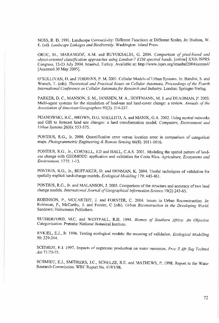
NOSS, R. D. 1991. Landscape Connectivity: Different Functions at Different Scales, In: Hudson, W.E. (ed). Landscape Linkages and Biodiversity. Washington: Island Press.

ORUC, M., MARANGOZ, AM. and BUYUKSALIH, G. 2004. Comparison of pixel-based andobject-oriented classification approaches using Landsat-7 ETM spectral bands. [online] XXth ISPRSCongress, 12-23 July 2004. Istanbul, Turkey. Available at: http://www.isprs.org/istanbuI2004/comm4/[Accessed 30 May 2005].

O'SULLIVAN, D. and TORRENS, P. M. 2001. Cellular Models of Urban Systems. In: Bandini, S. andWorsch, T. (eds). Theoretical and Practical Issues on Cellular Automata, Proceedings of the FourthInternational Conference on Cellular Automatafor Research and Industry. London: Springer-Verlag.

PARKER, D. C., MANSON, S. M., JANSSEN, M. A, HOFFMANN, M. J. and DEADMAN, P. 2003.Multi-agent systems for the simulation of land-use and land-cover change: a review. Annuals of theAssociation ofAmerican Geographers 93(2): 314-337.

PIJANOWSKI, RC., BROWN, D.G. SHELLITO, A and MANIK, G.A 2002. Using neutral networksand GIS to forecast land use changes: a land transformation model. Computers, Environment andUrban Systems 26(6): 553-575.

PONTIUS, RG., Jr. 2000. Quantification error versus location error in comparison of categoricalmaps. Photogrammetric Engineering & Remote Sensing 66(8): 1011-1016.

PONTIUS, R.G., Jr., CORNELL, lD and HALL, C.AS. 2001. Modeling the spatial pattern of land­use change with GEOMOD2: application and validation for Costa Rica. Agriculture, Ecosystems andEnvironment. 1775: 1-13.

PONTIUS, RG., Jr., HUFFAKER, D. and DENMAN, K. 2004. Useful techniques of validation forspatially explicit land-change models. Ecological Modeling 179: 445-461.

PONTIUS, RG., Jr. and MALANSON, l 2005. Comparison of the structure and accuracy oftwo landchange models. International Journal ofGeographical Information Science 19(2) 243-65.

ROBINSON, P., MCCARTHY, land FORSTER, C. 2004. Issues in Urban Reconstruction. In:Robinson, P., McCarthy, J. and Forster, C (eds). Urban Reconstruction in the Developing World.Sandown: Heinemann Publishers.

RUTHERFORD, M.C. and WESTFALL, R.H. 1994. Biomes of Southern Africa: An ObjectiveCategorization. Pretoria: National Botanical Institute.

RYKIEL, E.l, Jr. 1996. Testing ecological models: the meaning of validation. Ecological Modelling90: 229-244.

SCHMIDT, E.l 1997. Impacts of sugarcane production on water resources. Proc S Afr Sug TechnolAss 71:73-75.

SCHMIDT, E.l, SMITHERS, lC., SCHULZE, RE. and MATHEWS, P. 1998. Report to the WaterResearch Commission. WRC Report No. 419/1/98.

72

SCHULZE, R.E., LUMSDEN, T.G., HORAN, MJ.C. and MAHARAJ, M. 1999. Regional simulationanalysis of hydrological and yield responses of sugarcane under dryland and irrigated conditions.ACRUcons Report 28. Report to SASEX.

SINGH, A. 1989. Digital change detection techniques using remotely sensed data. InternationalJournal ofRemote Sensing 10(6): 989-1003.

SOUTH AFRICAN WEATHER SERVICES. 2005. [online]. Available at: lstweather.com.

[Accessed 25 May 2005].

THOMPSON, M. 1996. A standard land-cover classification scheme for remote-sensing applications inSouth Africa. South African Journal ofScience 92: 34-43.

TOFFOLI, T. AND MARGOLUS, N. 1987. Cellular Automata Machines: A New Environment forModelling. Cambridge: The MIT Press.

TURNER, B.L. and MEYER, W.B. 1991. Land use and land cover in global environmental change:considerations for study. International Social Science Journal 43: 669-679.

UMHLATHUZE MUNICIPALITY, 2002. Integrated Development Plan (IDP). [online]. Available at:http://devplan.kzntl.gov.zalMunicipaIlIDPs/uMhlathuze/idp_uMhlathuze_list.asp [Accessed 24 June2005].

UNITED NATIONS. 2004. Agenda 21. [online] United Nations. Available at:http://www.un.org/esa/sustdev/documents/agenda21/index.htm [Accessed 9 June 2005].

UNITED NATIONS POPULATION DIVISION. 2002. World Urbanisation Prospects: The 2001Revision [online]. Available at: www.un.org/popin/publications.html, [Accessed 03 September 2004].

VAN WYK, A. and SMITH, G. F. 1991. Regions ofFloristic Endemism in Southern Africa, A Reviewwith Emphasis on Succulents. Pretoria: Umdaus Press.

VELDKAMP, A. and FRESCO, L.O. 1996. CLUE: a conceptual model to study the conversion of landuse and its effects. Ecological Modelling 85: 253-270.

VERBURG, P.H., VELDKAMP, A. and FRESCO, L.O. 1999. Simulation of changes in the spatialpattern ofland use in China. Applied Geography 19: 211-233.

VERBURG, P.H., RITSEMA VAN ECK, J.R., DE NIJS, T.C.M, DIJST, M.l and SCHOT, P. 2004.Determinants of land-use change patterns in the Netherlands. Environment and Planning B: Planningand Design 31: 125-150.

VERBURG, P.H., SCHOT, P., DIJST, M. and VELDKAMP, A. In Press. Land-use change modeling:current practice and research priorities. [online] GeoJournal. Available at:http://www.geo.ucl.ac.be/LUCCIMODLUC_Course/PDF/T.%20Veldkamp%20(intro).pdf [Accessed24b June].

73

WAHBA, J. 1996. Urbanisation and migration in the third world, reproduced from Economic Review,14(2), [online] UK: University of Southampton. Available athttp://www.soton.ac.ukl~peters/er/jwI42.PDF [Acessed 17 May 2005].

WENG, Q. 2002. Land use change analysis in the Zhujiang Delta of China using satellite remotesensing, GIS and stochastic modeling. Journal ofEnvironmental Management 64: 273-284.

WHITE, R. and ENGELEN, G. 1993. Cellular automata and fractal urban form: a cellular modellingapproach to the evolution of urban land-use patterns. Environment and Planning A. 25: 1175-1189.

WILSON, E.O. 1994. The Diversity ofLife. London: Penguin.

WU, F. and WEBSTER, C. J. 2000. Simulating artificial cities in a GIS environment: urban growthunder alternative regulation regimes. International Journal ofGeographical Information Science 14(7):625-648.

WU, J., JENERETTE, G.D. and DAVID, J.L. 2003. Linking Land-Use Change With EcosystemProcesses: A Hierarchical Patch Dynamic Model. In: Guhathakurta (ed). Integrated Land Use andEnvironmental Models. London: Springer-Verlag.

WU, J. and QI, Y. 2000. Dealing with scale m landscape analysis: an overvIew. GeographicInformation Science 6: 1-5.

YANG, X. and LO, C. P. 2003. Modeling urban growth and landscape changes in the Atlantametropolitan area. International Journal ofGeographical Information Science 17(5): 463-488.

ZHA, Y., GAO, J. and NI, S. 2003. Use of normalized difference built-up index in automaticallymapping urban areas from TM imagery. International Journal ofRemote Sensing 24(3): 583-594.

ZIPPERER, W.C., WU, l., POUYAT, R.V. and PICKETT, S.T.A. 2000. The application of ecologicalprincipals to urban and urbanizing landscapes. Ecological Applications. 10(3): 685-688.

74

APPENDICES

Appendix 1 Table showing the land covers represented by the accuracy assessment ground truth points(In the match column, a one symbolizes a correct match and a two symbolizes anincorrect match)

WPno. Ground Truth Classification Match5 forestry forestry 16 forestry forestry 17 grasslands grasslands 18 sugarcane sugarcane 19 forestry grasslands 2

10 forestry grasslands 211 forestry grasslands 212 sugarcane forestry 213 sugarcane sugarcane 114 sugarcane industrial 215 sugarcane sugarcane 116 sugarcane sugarcane 217 forestry forestry 118 forestry forestry 119 forestry forestry 120 forestry grasslands 221 grasslands industrial 222 industrial industrial 124 waterbodies industrial 225 industrial industrial 126 industrial industrial 127 forestry forestry 128 forestry forestry 129 residential residential 230 residential residential 131 grasslands residential 232 residential residential 133 residential residential 134 residential residential 135 industrial industrial 136 grasslands residential 237 grasslands grasslands 138 grasslands grasslands 139 residential residential 140 industrial Industrial 141 industrial Industrial 142 industrial residential 143 grasslands sugarcane 244 grassfands grasslands 145 grasslands residential 246 grasslands grasslands 1

75

47 grasslands grasslands 148 sugarcane sugarcane 149 sugarcane sugarcane 150 sugarcane sugarcane 151 industrial industrial 152 industrial industrial 153 residential grasslands 2

76

An Assessment of Land Cover Changes Using GIS and Remote

Sensing: A Case Study of the uMhlathuze Municipality, KwaZulu­

Natal, South Africa

Thomas Robson, Fethi Ahmed, Trevor R. Hill

ii

ABSTRACT

Rapid growth of cities is a global phenomenon exerting pressure on land resources and

causing associated environmental and social problems. Addressing such problems through

sustainable use of land resources has become a pertinent issue since the Earth Summit in Rio

de Janeiro in 1992. An informed understanding of the processes and patterns of land cover

change will aid urban planners and decision makers in guiding environmentally conscious

development. The objective of this study was firstly, to determine the location and extent of

land use and land cover changes in the uMhlathuze Municipality, KwaZulu-Natal, South

Africa between 1992 and 2002 with the use of GIS and remote sensing, secondly, to predict

the likely expansion of urban areas for the following ten years, and thirdly, to ascertain the

usefulness of the techniques as tools for urban planners and policymakers. The uMhlathuze

Municipality has experienced rapid urban growth since 1976 when the South African Ports

and Railways Administration built a deep water harbour at Richards Bay, a town within the

Municipality. Three Landsat satellite images were obtained for the years, 1992, 1997 and

2002. These images were classified into six classes representing the dominant land covers in

the area. A post classification change detection technique was used to determine the extent and

location of the changes taking place. Thereafter, a GIS-based land cover change suitability

model, GEOMOD2, was used to determine the likely distribution of urban land cover ten

years later, in 2012. The model was validated using the 2002 image. Sugarcane was found to

have expanded by 129% between 1992 and 1997. Urban land covers had increased by an

average of 24%, whilst forest and woodlands had decreased by 29% between 1992 and 1997.

Variation in rainfall during the study years and diversity in sugarcane growth states had an

impact on the classification accuracy. Overall accuracy in the study was 74% and the

techniques gave a good indication of the location and extent of changes taking place within the

study site, and show much promise in becoming a useful tool for regional planners and policy

makers.

1

1. Introduction

1.1 Context

The United Nations Population Division (UNPD) (2002) estimate that the vast majority of

population growth expected over the next 30 years will occur in urban areas; that half the

world population will live in urban areas by 2007 and that the major population increase

between the years 2000 and 2030 will be absorbed by the urban areas of less developed

countries.

The expansion of urban areas brings dramatic changes in land cover and land use resulting in a

wide range of environmental impacts. These include soil erosion, reduction in water quality,

reduced plant biodiversity and pollution (Lubowski et aI, 2003; Bergeron & Pender 1999).

Land cover changes are also closely linked to global environmental change (Turner and

Meyer, 1991), and can result in a decline or loss of spatial extent and connectivity of wildlife

habitats (Leao et aI, 2004), leaving landscapes fragmented, and reducing the distribution of

many species to small isolated populations (Wu et aI, 2003). Furthermore, many impacts of

land cover change, such as land disturbance, formation of urban heat islands and modifications

in nutrient dynamics, will alter local climates, often preventing re-habitation of the original

species (Zipperer et aI, 2000).

Although there is a paucity of detailed studies dealing with urban ecosystems (Wu et aI, 2003),

they play a number of important roles, such as air filtration, reduction of pollution, climate

regulation and sewerage treatment (Elmqvist et aI, 2004), all of which play a vital role in

sustaining a healthy living environment and preserve ecological processes. Barredo et al

(2004) point out that urban areas have to maintain an equilibrium between economic activities,

population growth, and pollution and waste so that the urban system and its dynamic processes

can evolve with minimal impacts on the environment. Deal (2001) extends this point and

explains that ecological urban sustainability requires the implementation of ecologically sound

alternatives to current practices.

2

Verburg et al (2004) discuss five dominant determinants of land use change: spatial policies,

economic factors, biophysical constraints and potentials, social factors and spatial interactions.

These factors interact to produce prevailing patterns of land uses and must be considered in

determining the future course of land use changes.

Braissoulis (2001) notes that the relationship between land cover changes and large-scale

environmental problems, such as climate change, has elevated the field as an important subject

of policy disciplines. The expanding relevance of the field has also increased the need for

research into the analysis of land use and land cover change as a step towards mitigating future

environmental disasters. The development of both methods of analysis and data will lead to

more informed decision-making for both planners and policy-makers alike (HeroId et aI,

2003).

Land use and land cover changes take place in response to a variety of factors stemming from

human needs and wants. These influence the extent, pattern and rate of such changes at both

the macro and micro level, and accordingly need consideration in any study of land use and

land cover changes. Furthermore, studies should conceptualise the interactions among the

driving forces of land-use change, their mitigating procedures and human behaviour and

organisation (Verburg et aI, 2004), and should not be viewed independently of the driving

forces underlying the motivation for such changes.

1. 2 Land Cover Change Detection

The use of Geographic Information Systems (GIS) and remote sensing enables analysis of the

spatial components of the earth's surface. Remotely sensed imagery, firstly, allows for detailed

and consistent measurements on the earth's surface conditions at high temporal frequencies

(Gibson, 2000), and secondly, allows for easy differentiation between land covers based on

their reflectance values, and hence can reveal areas that have undergone changes in land cover

over time. Remotely sensed imagery has been used extensively for land cover applications

such as the analysis of land cover dynamics, damage mapping, risk assessment, urban

3

expansion assessment and ecosystem monitoring (Bruzzone & Cossu, 2002; Civco et al 2002;

Weng 2002; Chen et a12003; Coppin et ai, 2004).

For temporal studies it is crucial that satellite imagery undergo a preprocessing stage to ensure

consistency between the reflectance values and registration of the different images in the time

sequence. This stage entails the corrections of radiometric and atmospheric deficiencies and

the removal of flaws (Mather, 1989). For temporal change studies this stage involves image

registration to ensure comparability between dates (Lu et ai, 2004). Using similar dates for the

anniversary images increases the comparability of the images by improving the likelihood of

similar sun angles, soil moisture condition and plant phenological state (Singh, 1989; Jensen,

2000).

1. 3 Predictive Change Modelling

Land Use and Cover Change LUCC models are effective tools designed to analyse the

consequences and causes of land use dynamics, to aid in investigating and understanding

landscape processes and to analyse the underlying socio-economic processes (Verburg et ai, in

press). Most LUCC models are developed from a GIS base and have been applied to various

applications. These include urban growth, the analysis of interactions of natural processes, the

spatial consequences of policy decisions and proposed management strategies, agricultural

expansion, deforestation and the effects of land use on the release of carbon into the

atmosphere (Baker, 1989; White & Engelen, 1993; Hall et ai, 1995; Pontius et ai, 2001;

Barredo et ai, 2004).

Most LUCC models utilize Cellular Automata as a fundamental component allowing them to

model changes on a spatial plane. The process of Cellular Automata is based on a lattice

framework of congruent cells (Parker et ai, 2003) relating well to spatial analysis. Land

conversion takes place through a series of transitions in which pixels change from one land

cover to another according primarily to the land cover of ~he neighbouring pixels (Toffoli &

Margolus, 1987). All the pixels are interdependent relational entities updated simultaneously

as the lattice develops in discrete time steps (Deal, 2001). Transition rules that reflect the

4

drivers such as land suitability, urban zones and protected areas, guide these conversion by

determining the likelihood of each pixel to undergo change.

The majority of LUCC models, especially those designed for urban growth, have been

produced in developed countries, particularly the United States, where there is both the

expertise and the necessary data (Leao et ai, 2004). As noted earlier, it is likely that the less­

developed countries will experience the majority of urban growth and consequently such

models have important application in these regions. However, Leao et ai (2004) point out that

urban growth in developed and developing countries often takes place in different patterns,

which may impact the effectiveness of such models to developing countries.

This study used the GIS-based model GEOMOD2 (Pontius et ai, 2001), which predicts the

likely locations of land cover changes from one class to another. The model is primarily based

on Markov Chain Analysis and Cellular Automata, and simulates the spatial patterns of land

use change based on the patterns of biogeophysical attributes and existing land uses derived

from digital raster maps. (Hall et ai, 1995). The predictive model simulates the pattern and

locations of land use change and not the quantity, which must be obtained from another

source.

2. Study Site

The uMhlathuze Municipality is situated on the north coast of KwaZulu-Natal, South Africa

between latitudes 28°37'S and 28°57'S, and longitudes 31°42'E and 32°09'E (figure 1). It

comprises the towns and settlements of Richards Bay, Empangeni, Esikhawini, Ngwelezane,

Nseleni, and Felixton (Anon, no date).

The uMhlathuze Municipality covers an area of 796 km2, with a population of 296 339 at an

average of 372 people per km2• An estimated 169 008 of these people are resident in urban

areas and 41 % are between the ages of 15 and 34 years. The total unemployment rate in the

area is 41 %, although this figure only relates to the formal sector. (Anon, no date)

5

5...... 10 15 Kilometers

Location of KZN within South Africa

LEGEND_ Waterbodies~ Local Municipalfties~ uMhalthuze Municipality~ KwaZulu-NatalD Provincial Boundary

Fig 1. Location ofurban areas, settlements and lakes in the uMhlathuze Municipality.

The uMhlathuze Municipality is recognised as having high conservation significance in terms

of biodiversity (uMhlathuze IDP, 2002) and is situated within the Maputaland Centre of

Endemism (van Wyk & Smith, 2001). The dune ridge running along the coast is considered a

particularly important corridor for genetic exchange between members of certain species from

different biogeographical units. This is the only remaining passageway as the majority of

inland vegetation has been converted to sugar cane (uMhlathuze IDP, 2002).

The Town of Richards Bay has a scattered structure with many ofthe large industries sparsely

distributed within areas of natural vegetation, lakes and wetlands. This allows for habitat

connectivity between the industries. Similarly, the many settlement areas within the

Municipality comprise well-spaced settlements with patches of subsistence crops and

grassland between the dwellings. Often there are no streets and only footpaths between

dwellings.

6

In the late 1960s, the town of Richards Bay was transformed from a small fishing village when

South African Railways and Harbours Administration acted on the need to build a deep-water

harbour on the eastern coast of South Africa to accommodate large vessels. The development

of the town was part of a National Development Plan linking the harbour to inland

developments by rail (Department of Planning, 1972). Following this, the area underwent

rapid transformation with the growth of urban areas, containing large industrial, commercial

and residential components. The town has become an important growth node as a consequence

of several government-driven economic policies over the years, including the decentralisation

policy during the Apartheid years and the Spatial Development Initiative (SDI) programme in

more recent times (Hall, 2000).

Changes in the uMhlathuze Municipality are a consequence of both First and Third World

processes. Richards Bay is based on an industrial foundation with large extractive industries as

described above, supporting an affluent society in the formal sector. However, Richards Bay

also contains a very large element of what Hall (2004) describes as a city coping with informal

hypergrowth. Many cities in sub-Saharan Africa fall into this category and are characterised

by rapid population growth from migration and natural increase and supporting economies

heavily dependent on the informal sector. Such cities contain extensive informal housing

areas, with widespread poverty and environmental and health problems. Richards Bay contains

both the formal and informal sectors integrated together to provide the prevalent trajectories of

growth.

The uMhlathuze Municipality has experienced much of its growth through urban sprawl with

scattered low-density housing in informal settlements surrounding Richards Bay. The large

industrial base attracts many people to the area with the prospect of possible jobs and they

seek accommodation in the informal housing market. Barredo et al (2004) point out that when

population growth takes place in loosely planned urban structures, environmental and social

consequences can be significant, particularly in areas that have undergone rapid growth. Since,

in most developing countries, urban development is concentrated on the needs of the poor

(Robinson et aI, 2004), environmental considerations are often neglected if not properly

planned for.

7

3 Methods

3.1 Data

Three Landsat satellite images representing the years 1992, 1997 and 2002 were obtained for

the months of July, August and October respectively. Landsat -5 and -7 were used as they

provide imagery at a 30m spatial resolution in the multi-spectral bands. The images were from

as similar seasons as possible to maintain consistency of environmental variables and reduce

problems resulting from seasonal changes, such as different sun angles and changes in plant

phenology (Singh, 1989; Jensen, 2000). To ensure comparability and to prevent spatial errors

occurring during the analysis process, the three images were re-projected to a Transverse

Mercator projection with a Cape datum and a Clarke 1880 spheroid. They were then

geometrically corrected and co-registered to represent precisely the same areas on the ground.

Further pre-processing of the images, such as radiometric calibration has been carried out prior

to my receiving them.

The images were subset to the uMhlathuze municipal boundary without including coastal

sand, since this had undergone minimal changes during the study period, and the low

reflectance of sand caused confusion with the urban land covers in the classification process.

For the same reason, large riverbeds on the inland boundaries of the Municipality were

excluded.

3.2 Land Cover Change Detection

Several methodologies and algorithms have been devised for land cover change detection

(Singh, 1989; Jensen, 2000; Coppin et ai, 2004). Choice of these depends primarily on

biophysical characteristics of the study site and the precision of the image registration (Jensen,

2000). For this Study, a 'post classification comparison' change detection technique (Singh,

1989) was used, due to the variability in rainfall in the study area and use of imagery from

different Landsat satellite series. This technique involves the comparison of independently

produced classified images, and hence reduces the impacts of the factors mentioned above.

8

Furthermore, by classifying the images separately one minimises the need for accurate

radiometric calibration between different dates (Coppin et aI, 2004). However, such an

approach relies on the accuracy of the initial image classifications as misclassifications at this

stage are compounded when multiple images are compared (Jensen, 2000).

A combination of bands 2 (green), 3 (red) and 4 (near infrared) were found to be the most

suitable to distinguish between the relevant land features, and have been used for such land

features in similar studies (Weng, 2002; Zha et aI, 2003). Classification was carried out with a

'supervised classification' process using a 'maximum likelihood' decision rule, which divided

the area into land cover classes based on the spectral properties of user defined training sites.

The training sites were developed and verified with the aid of recent land use maps, aerial

photographs and visits to the study area. The three satellite images were classified separately

using consistent land cover classes developed from the South African land cover classification

scheme (Thompson, 1996).

A total of seven classes was chosen to avoid complications arising from too many classes

whilst still depicting the relevant differences in land cover. The categories were; commercial/

industrial built-up land, residential built-up land, forest and woodlands (comprising both

natural forest and commercial forestry), grasslands, sugarcane, waterbodies, and mines and

quarries. The classified images were filtered with a 3 x 3 statistical filter to reduce individual

misclassified pixels within uniform land cover areas. In addition, large rivers in the area were

digitized and automatically classified as waterbodies as the sand in the river caused confusion

in the classification as stated earlier.

An accuracy assessment was only attempted for the 2002 image due to a lack of earlier

reference data. This image itself was to some extent out of date (study carried out in early

2005), but, from personal observations, it was considered comparable to the present land

covers in the uMhlathuze Municipality. Consequently, it was critical that ground truth points

were only taken in areas where it was presumed the land cover had not changed since 2002. A

total of 48 ground truth points was recorded with the use of a Global Positioning System

9

(GPS). The sample was attempted to be both representative and random but was limited by

access, security and time constraints.

Classified images were compared on a pixel-by-pixel basis, difference images and change

matrices were produced to determine the locations, rate and extent of changes.

3.3 Predictive Change Modelling

A GIS-based land cover change model GEOMOD2 was used to produce a predictive image

for the year 2012 showing the likely extent of urban land covers. The output image was based

on the location of land covers in 2002 and the changes that took place between 1992 and 2002.

The model simulates change between only two land cover classes and therefore the classes

used in the change detection section were combined together to form two appropriate classes.

The classes forest and woodlands, grasslands, sugarcane, waterbodies, and mining and

quarries were reclassified to non-built-up and the land cover classes commercial/industrial

built-up and residential built-up were reclassified to built-up. The class mining and quarries

was included in the non-built-up class, as it did not represent an urban land cover.

A suitability image was created to stipulate the areas most likely to undergo transformations.

This image is an important decision rule in the model designed to guide the model to predict

land cover changes according to realistic system behaviour (Wu & Webster, 2000). The choice

of criteria was based on previous studies (Hall et aI, 1995; Deal, 2001; Parker et aI, 2003;

Barredo et aI, 2004; Yang & Lo, 2003), the availability of data and the ability of the model

itself. The criterion used was the uMhlathuze Municipality's demarcation of urban zones, and

the constraints included large waterbodies, areas within a proximity of 40 m to the centre of

large rivers and areas zoned as protected. These factors were integrated with a Multi-Criteria

Evaluation (MCE) process to produce a single composite raster image for input into the model.

10

The quantity of land predicted to be under built-up land cover in 2012 was calculated from the

expansion rate that took place between 1992 and 2002 as observed in the classified images of

these dates.

Model validation was carried out using a simulated image for 2002 since there was no

reference image for 2012. This image was created using the 1992 image as the base image, the

same suitability image used in the 2012 simulation and the known quantity of changed pixels

between 1992 and 2002. This image was then compared to the 2002 reference image using the

VALIDATE function in Idrisi (Clarke Labs, 2003).

4. Results

4.1 Classification

The classification results indicate the distribution of the land covers in the three years (figures

2 to 4). It is likely that seasonal differences in the images (1992 in July, 1997 in August and

2002 in October) impacted this process due to different growth states of the vegetation classes.

Waterbodies in the study area generated a large variety of reflectance values, due to different

depths, salinity and clarity levels and extent of vegetation cover. To avoid confusion with

other classes, these areas were digitised and automatically classified as waterbodies.

In several areas sugarcane had been harvested, leaving fields with bare earth generating

similar reflectance values to urban areas. To reduce this problem several sugarcane classes

were created to represent the different levels of sugarcane cover, and these were grouped to

form one single sugarcane class. Nevertheless, a few dispersed urban class pixels still

remained in sugarcane areas and correspondingly a few dispersed sugarcane pixels appeared

in urban areas.

4.2 Accuracy Assessment

An error matrix was created to determine the classification accuracy (table 1) of which the

results are provided in table 2. The overall accuracy was 74% indicating that the accuracy was

11

moderately good and that 74% ofthe overall classification is likely to be correct. However, the

result was not at the minimum standard stipulated by the USGS classification scheme of 85%

(Anderson et al, 1976).

The producer's accuracy had a wide range between the different classes from 100% for

sugarcane and residential built-up to 55% for grasslands. The classes sugarcane and

residential built-up were thus accurately interpreted and can be easily mapped on the earth's

surface. The classes grasslands and commercial/industrial built-up can be mapped with less

confidence. The user's accuracy also varied greatly between classes from 64% in the forest

and woodlands class to 100% in the commercial/ industrial built-up class. This result indicates

that the classes commercial/industrial built-up and residential-built-up successfully represent

what users of the data can find on the ground (Story & Congalton, 1986).

Table I Classification error matrix for the 2002 classified image

;[ota1Q) 11C)

7 1C'CI 9E 6 4 10Q)(J 1 6 7c:Q) 9 9....! 1 1Q)

IX: 7 11 6 15 0 47

F -forest and woodlands R -residential built-upS -sugarcane CII -commercial/industrial built-upG -grasslands W -waterbodies

Table 2 Statistical results from the classification error matrix of the 2002 classified image

Land cover Producer's accuracy User's accuracyF 88% 64%S 100% 78%G 55% 60%R 100% 86%CII 60% 100%

Overall accuracy =(7 + 7 + 6 + 6 + 9) 147 =74%

12

4.3 Post Classification Change Detection

Classified images of the study area cover a total of 79 026 ha and contain the classes

commercial/industrial built-up land, residential built-up land, forest and woodlands,

grasslands, sugarcane, waterbodies and mines and quarries The 2002 image is the only one

that contains the mines and quarries class, since mining in the area began after 1997. Figures

2, 3 and 4 illustrate the location and extent of the land cover classes in the years 1992, 1997

and 2002 respectively. The number of ha covered by each of the land covers and their

respective proportions are presented in table 3. Figure 5 illustrates the land cover changes

graphically.

Transverse MecatorCental Meridian 31 East

Clar1l.e 1880 Spheroid

Fig. 2. Classified image of the uMhlathuze Municipality in 1992.

N

A

Land Covers

..ComlnOf"cial' indu$trial built up

CEJ Resldantial bull up

.. Forest end woodL:mds

o G......"".

~Sugareane

"WaWrt:lOdies

~ Mines and quarries

Transverse MecatorCental Meridian 31 East

Clarke 1880 Spheroid

1.5

""''''''''iiiiil'''!'!''''''''''''''iiiiiiiiiiiiii Kilornelers

N

A

Land Covers

..Commercial! industria! built up

~ Residential built up

..Forest and woodlands

c=JGrasslands

B1I Sugarcane

"Waterbodies

..Mines and quarries

13

Fig. 3. Classified image ofthe uMhlathuze Municipality in 1997.

Transverse MecatorCentalMeridian 31 East

Clarke 1880 Spheroid

": ~~~j,

1.5 0

"'''''''iiii''''''''''''''''''''iiiiiiiiiiiiiKilometers

~".~

N

A

Land Covers

_ Commercial I lndusbial buirtup

~ResldentlalbUlltup

..Forest and woodlands

c:::J Grass!ands

III Sugarcane

~Waterbodies

"Minesandquarries

Fig. 4. Classified image of the uMhlathuze Municipality in 2002.

14

Figure 3 clearly shows that the uMhlathuze Municipality has undergone considerable change

during the ten years of the study and most of this change occurred between 1992 and 1997.

The biggest change was found in the sugarcane class, which increased by 8114ha (129%)

between 1992 and 1997 but then decreased by 1146 ha (8%) between 1997 and 2002.

Commercial/industrial built-up land experienced an overall increase from 1992 to 2002 of

611 ha, a growth of 23%. Residential built-up land increased between 1992 and 2002 by 1204

ha, a growth of 25%. The forest and woodlands class underwent a large decrease from 1992 to

1997 of 8098 ha (29%). It then increased by 838 ha (4%) from 1997 to 2002. Grasslands,

although shifting spacially, remained fairly constant in terms of overall quantity with a small

decrease of2206 ha (7%).

Table 3 Area, change and percentage change of the land covers in the three study years

1992 Change (92·97) 1997 Change (97-02) 2002 Change (92-02)

(ha) Chance (ha) % of 1992 (ha) Chance (ha) % of 1997 (ha) Chance (ha) % of 1992C/lndustrialbuilt-up 2653 ·103 -4 2550 714 28 3264 611 23Residentialbuilt-up 4876 460 9 5336 744 14 6080 1204 25Forest &woodland 27930 -8099 -29 19832 838 4 20670 ·7260 -26

Grasslands 32855 -228 -1 32628 -1979 -6 30649 ·2206 -7

Sugarcane 6314 8113 128 14428 -1146 ·8 13282 6967 110

Water bodies 4397 -144 ·3 4253 263 6 4516 119 3

Mining 0 0 0 565 565 565

Total 79026 79026 79026

II

j

15

45.,-------------------------

40 f--------------{h

35 f-----=-----------jI"7r---

:;;0 f--------Y IJ--------J';I­';25 f--------H-~O -!-------------11"/.

"..o~ 15 -!-----------'V.....

10 -!----------Io'

5+------1'

o

12J 1992-­

-1-------1 ~ 1997--

-1-------102002--

Urban UrbanIndustrial Residential

Forestry Grasslands Sugarcane Waterbodies

LandcQver Classes

Mining

Fig. 5. Graphical representation ofthe land cover changes in the uMhlathuzeMunicipality between 1992 and 2002.

The large increase in sugarcane between 1992 and 1997 (129%) is concentrated in the area to

the north of Empangeni. It is primarily a consequence of the Heatonville irrigation scheme,

developed by Tongaat-Huletts in 1994, which allowed for a large area previously under the

rain shadow of a mountain range to be irrigated cost effectively (Fortman, 2005 pers comm.).

Agriculture that relies on irrigation has many environmental impacts in terms of water

resources, such as the depletion of supplies to downstream areas, modified flow regimes and

re-channeling of stream networks. An increase in small-scale cane growers in South Africa in

recent years (Maloa, 2001) may have impacted on this result.

The results of the change matrices (Appendix A) reveal that much of the land converted to

sugarcane was formerly grasslands (7 704 ha) and forest and woodland (1 782 ha). This

suggests that the expansion of sugarcane has reduced the extent of Coastal Bushveld­

Grassland vegetation type, which had already been greatly transformed by agriculture (Low &

Rebelo, 1998).

The commercial/industrial built-up and residential built-up land covers showed average

increases of 23% and 25% respectively over the ten year period. There is clear evidence of

expansion of residential-built up areas in the northern parts of Richards Bay and in the

township areas of Esikhawini and Felixton, in the southern part of the Municipality. The

16

industrial nature of Richards Bay demands large labour resources, which, when coupled with

high levels of poverty in surrounding areas, draws many people to the area. The increase in

commercial industrial built-up is mainly concentrated around the harbour and the town centre

of Richards Bay. Industries are attracted by economic policy, the deep-water harbour and good

industrial infrastructure.

In the case of forest and woodlands, this class demonstrated a substantial decrease between

1992 and 1997 of 8098 ha (29%), followed by a small increase of 838 ha (4%) between 1997

and 2002. The change matrices (table 4) confirms that most of the forest and woodland areas

were converted to grasslands (8 367 ha) and sugarcane (1 782 ha) during the study period.

There is clear evidence, along the coast in the southern regions of the uMhlathuze

Municipality, that large tracts of natural forest have been converted to grasslands. Clearing of

forest patches is common practice in South Africa where wood is cut for fuel and to increase

grazing capacity.

The change matrices (table 4) revealed that many areas changed from both grasslands toforest

and woodlands (119 ha) and from forest and woodlands to grasslands (279 ha). This indicates

that spatial shifting has occurred. In some areas, forest patches have expanded into the

grasslands while in others, forests patches have either died back, been cleared or converted to

grasslands. Forest expansion in South Africa is often the result of the invasion of alien trees

such as Eucalyptus and Acacia species. These plants negatively transform ecosystems by

consuming resourses excessively and altering microclimates, in turn changing biochemical

cycles (Richardson & van Wilgen, 2004).

Open cast titanium mining began in the Municipality in 2001 and therefore is only evident in

the 2002 image. The mining operations cover an area of 565 ha (0.7% of the total

Municipality), which was previously sugarcane or and grasslands (198 ha and 224 ha

respectively).

17

4.4 Predictive Change Modelling

The model appears to have simulated the spread of built-up land in a logical manner consistent

with the spread of the built up classes in the 1992, 1997 and 2002 images (figures 6 to 8).

Figure 9 displays regions where GEOMOD2 predicted the change to take place in black. The

majority of change has occurred around existing urban areas, spreading out into the adjacent

land covers. The model has also predicted a densification of the existing built- up areas where

there is much undeveloped land within built-up areas.

Fig. 6. Location of built-up land cover (white areas) in 1992 [lcrn = 5krn].

18

Fig. 7. Location of built-up land cover (white areas) in 2002 [lcm = Skm].

Fig. 8. Location of predicted built-up land cover (white areas) in 2012 as derived from GOEMOD2 [lcm = Skm].

19

Fig. 9. Image illustrating the locations where GEOMOD2 predicted the increase in built-up land cover to takeplace (Illustrated by black regions) [lcm = 5km].

4.5 Model Validation

The results of the model validation quantify the positional differences between the 2002 model

output and the reference image. Figure 10 displays (in black) the areas classified differently

between the model output image and the reference image. Much of the difference is not in

close proximity to the urban centres of Richards Bay, Empangeni, Esikhawini, Ngwelezane,

Nseleni, and Felixton. This is a consequence of the 2002 classified image (reference image)

containing small pockets of incorrectly classified built-up pixels within the non-built-up land

covers resulting from patches of bare earth within cultivated lands, rather than the model

having produced an inaccurate prediction.

20

Fig. 10. Image illustrating the difference in location of built-up between the GEOMOD2 produced image and thereference image (areas of difference shown in black) [Icm = Skm].

The relevant results from the validation process included a Kappa for no information

(indicating the proportion of pixels classified correctly relative to the expected proportion

classified correctly by a simulation with no ability to specify accurately quantity or location)

and a Kappa for grid-cell level location (indicating how well the grid cells are located on the

landscape), both providing a result of 0.9121. This result proves the images to be a very near

match. However, the result is rather misleading as the 'VALIDATE' process incorporates the

entire image, rather than simply the cells in which GEOMOD2 had predicted change. Since

the area that underwent change was a very small proportion of the whole image, this result is

largely inconclusive in terms of providing an indication of the accuracy of GEOMOD2 to this

application. A simple visual analysis of figure 10 may provide a clearer indication of the

effectiveness of GEOMOD2 in predicting the location of change in this study.

21

4. 6 Limitations to the Study

Rainfall had an impact on this study as it affects the growth state and quantity of vegetation,

altering the spectral response of vegetation land covers. The three years of this study

experienced rather varied rainfall. In 1992 the total was 753.9 mm, 58% of the annual average,

in 1997 the total was 2154.5 mm, 167% of the average and in 2002 the total was 986.2 mm,

76% of the average (South African Weather Services, 2005). Ideally, the three images need to

contain consistent growth states, but with such varied rainfall between image dates this was

difficult to achieve. Accordingly, the use of a 'post classification comparison' change

detection technique reduced the impacts of such variability across dates.

The difference in rainfall quantity during the study years is presumed to have impacted the

classification process in several ways. Firstly, higher rainfall increases the areas of all the

vegetation classes and thus decreases the area of the non-vegetation classes such as

commercial/industrial built-up and residential built-up. This trend was prevalent in the results

as the urban industrial class decreased from 1992 to 1997 by 4% (103 ha) and then showed a

large increase of 28% (714 ha) from 1997 to 2002. Similarly in the Urban Residential class

only increased by 9% (460 ha) from 1992 to 1997 and then increased by 14% (744 ha) from

1997 to 2002. The impact of this trend on the waterbodies class is inconclusive since a mask

was used to remove the main waterbodies from the analysis. Nonetheless, this class did show a

decrease in size in the 1997 image, resulting from changes in unmasked waterbodies.

During the 1997 image it is likely that the grassland training sites contained a larger amount of

bare earth and dry grass giving these areas a higher reflectance value. This caused some

residential built-up areas to be classified as grasslands.

The high vegetation growth in the suburbs and spatially dispersed nature of both the large

industries around Richards Bay and the settlement areas also negatively impacted on the

classification accuracy giving a 'salt-and-pepper' type classification result. In these situations

approaches such as object-oriented classification, which takes the form, textures and spectral

information into account (Oruc et ai, 2004), may produce more accurate results. Various

22

filtering techniques can also reduce such problems. Furthermore, imagery with a finer

resolution would also reduce this effect.

Shadows also affected the classification process. Where plantations were very tall, adjacent

areas would lie under shadow and have reflectance values similar to commercial/industrial

built-up or waterbodies. This was another source ofpixel misclassification.

5. Conclusion and Recommendations

5.1 Changes in the uMhlathuze Municipality

The most significant change in the uMhlathuze Municipality was the increase in sugarcane,

which increased by 6 967 ha (110%) between 1992 and 2002. This transformation may have

improved the economy of the region but has, at the same time, reduced the extent of Coastal

Bushveld-Grassland vegetation type, which is already greatly transformed by such agricultural

practices (Low & Rebelo, 1998). Mitigation measures may include the provision of corridors

of natural vegetation allowing for species migration between conserved areas. The rapid rate

of many of the changes exemplifies the need for such measures.

Since many of the built up areas around Richards Bay are industrial in nature, the increase in

this land cover is of particular concern. The spread of large industries results in environmental

problems such as air, groundwater and riparian pollution. Consequently, it is imperative that

planning strategies incorporate such considerations to guide the development in a way to

minimise these impacts in the future.

The loss of coastal forest in the southern parts of the uMhlathuze Municipality is of concern

because the coastal dunes of KwaZulu-Natal are prime areas for residential development, and

the vegetation is being destroyed at an alarming rate. Moreover, the uMhlathuze IDP (2002)

notes that the dune ridge along the coast is a particularly important corridor for genetic

exchange between certain species from different biogeographical units. It is the only

remaining passageway as the majority of inland vegetation has been converted to sugarcane.

23

5.2. Success o/the Study

The various stages of growth of the sugarcane fields including fallow fields, the large amount

of vegetation in the suburbs, the spatially distributed nature of both the industrial areas and the

townships, and the shadows along the edges of plantations, all caused confusion in the

classification results, and therefore contributed a low classification accuracy (74%). This is

considered detrimental to the Post Classification Comparison algorithm as the final accuracy is

a multiplication of the accuracies of the individual classified images (Coppin et aI, 2004).

Notwithstanding these problems, the change analysis provided a good indication of the

changes that have taken place in the Municipality between 1992 and 2002. The techniques can

be considered successful as the large scale of the study site meant that, in spite of certain

inaccuracies, the general locations and rates of changes were clearly demonstrated.

Policy, economic fluctuations and large industrial projects have all had a significant impact on

the growth and development of urban areas, especially around Richards Bay (Hall, 2000).

GEOMOD2 was not designed as an urban growth model but rather as a LUCC model and thus

unable to incorporate such factors. Other models such as the SLEUTH urban growth model

(HeroId et aI, 2003) may have been better suited to the urban growth part of this study as they

better facilitate the incorporation of such factors. However, such models require additional

data that was available for this study.

Furthermore, the model did not include representation of some important socio-economic

factors such as human decision-making (Parker et aI, 2003), which, in Richards Bay where

development is guided through a Structure Plan framework, would improve the accuracy of

the model.

Overall the study provided valuable results for both the study site and the techniques used. In

determining the change in land cover between 1992 and 2002, the method indicated clearly

where the major changes were taking place, and the extent and nature of the changes, while

24

the GEOMOD model produced a good prediction of the extent of urban land covers that can

be expected in 2012.

25

References

Anderson, lR., Hardy, E.E., Roach, IT. and Witmer, R.E. (1976). A land use and land coverclassification system for use with remote sensor data. US Department ofthe Interior.Geological Survey, Professional Paper 964.

Anonymous. (no date). Key statistics on the uMhlathuze municipal area [online]. City ofuMhlathuze Available at:http://www.richemp.org.zaltulipuMhlathuzeInternetlrepository/Pdfs%20and%20Presentations/Demographics.pdf [Accesses 7 June 2005].

Baker, W.L. (1989). A review of models of landscape change. Landscape Ecology, 2(2), 111­133.

Barredo, 1 1., Demicheli, L., Lavalle, C., Kasanko, M. and McCormick, N. (2004). Modellingfuture urban scenarios in developing countries: an application case study in Lagos, Nigeria.Environment and Planning B: Planning and Design, 32,65-68.

Bergeron, G. and Pender, 1 (1999). Determinants ofland use change: Evidencefrom acommunity study in Honduras. EPTD Discussion Paper No. 46 [online]. Washington:International Food Policy Research Institute. Available athttp://www.ifprLorg/divs/eptd/dp/papers/eptdp46.pdf [Accessed 04 October 2004].

Briassoulis, H. (2001). Policy-orientated integrated analysis of land-use change: an analysis ofdata needs. Environmental Management, 27(1), 1-11.

Bruzzone, L. and Cossu, R. (2002). Analysis ofmultitemporal remote sensing images forchange detection: Bayesian thresholding approaches. Technical Report #DIT-02-0031[online]. Italy: Department ofInformation and Communication Technology. University ofTrento. Available at http://www.dit.initn.it.

Chen, Z., Chen, l, Shi, P. and Tamura, M. (2003). IHS-based change detection approach forassessment of urban expansion impact on arable land loss in China. International Journal ofRemote Sensing, 24(6), 1353-1360.

Civco, D.L., Hurd, J.D., Wilson, E.H., Song, M. and Zhang, Z. (2002). A comparison oflanduse and land cover change detection methods. [online]. Proceeding of the ASPRS-ACSMAnnual Conference and FIG XXII Congress. Available at:http://resac.uconn.edu/publications/tech-papers/pdf-paper/Land_Cover_Change_ASPRS2002.pdf [Accessed 23 June 2005].

Coppin, P., Jonckheere, 1., Nackaerts, K., Muys, B. and Lambin, E. (2004). Digital changedetection methods in ecosystem monitoring: a review. International Journal ofRemoteSensing, 25(9), 1565-1596.

Deal, B. (2001). Ecological urban dynamics: the convergence of spatial modeling andsustainability. Building Research and Information, 29(5),381-393.

26

Department of Planning (1972). Richards Bay Urban Development Plan. Pretoria: Departmentof Planning

Elmqvist, T., Colding, 1., Barthel, S., Borgstrom, S., Duit, A., Lundberg, J., Andersson, E.,Ahrne, K., Ernstson, H., Folke, C. and Bengtsson, 1. (2004). The Dynamics of social­ecological systems in urban landscapes; Stockholm and the National Urban Park, Sweden.Annuals ofthe New York Academy ofScience, 1023,308-322.

Fortman, T. (2005). Personal Communication. SASRI extension officer for Felixton Mill.

Gibson, P.J. (2000). Introductory Remote Sensing: Principles and Concepts. London: RoutledgePublishers.

Hall, c.A.S., Tian, H., Qi, Y., Pontius, G. and Cornell, 1. (1995). Modeling spatial andtemporal patterns of tropical land use change. Journal ofBiogeography, 22, 753-757.

Hall, P.V. (2000). Regional development and institutional lock in: a case study of RichardsBay, South Africa. Critical Planning, 7,87-102.

Herold, M., Goldstein, N.C. and Clarke, K.C. (2003). The Spatiotemporal form of urbangrowth: measurement, analysis and modeling. Remote Sensing ofEnvironment 86: 286-302.

Jensen, 1.R (2000). Remote Sensing ofthe Environment: An Earth Resource Perspective. NewJersey: Prentice Hall.

Leao, S., Bishop, I. and Evans, D., (2004), Simulating Urban Growth in a Developing Nation'sRegion Using a Cellular Automata-Based Model. Journal ofUrban Planning andDevelopment, 130(3), 145-158.

Lu, D., Mausel, P., Brondizio, E. and Moran, E. (2004). Change detection techniques.International Journal ofRemote Sensing, 25,2365-2407.

Lubowski, RN., Plantinga, AJ. and Stavins, RN. (2003). Determinants ofland-use change inthe United States 1982-1997. Paper preparedfor presentation at the Association ofEnvironmental and Resource Economists (AERE) sessions ofthe American AgriculturalEconomics Association (AAEA) annual meeting Montreal, Canada [online]. Washington:Resources for the Future. Available at: http://www.rff.org [Accessed 04 October 2004].

Maloa, M.B. (2001). Sugar cane: a case as development crop in South Africa. Paperpresented at the SARPN conference on Land reform and Poverty Alleviation in South Africa.Pretoria [online] South Africa: South African Regional Poverty Network. Available at:http://www.sarpn.org.za/EventPapers/Land/20010605Maloa.pdf [Accessed 06 May 2005].

Mather, P. M. (1989). Computer Processing ofRemotely Sensed Images, An Introduction.Guildford: BiddIes Ltd.

27

Oruc, M., Marangoz, A.M. and Buyuksalih, G. (2004). Comparison ofpixel-based and object­oriented classification approaches using Landsat-7 ETM spectral bands. [online] XXth ISPRSCongress, 12-23 July 2004. Istanbul, Turkey. Available athttp://www.isprs.org/istanbuI2004/comm4/ [Accessed 30 May 2005].

Parker, D. C., Manson, S. M., Janssen, M. A., Hoffmann, M. 1. and Deadman, P. (2003).. Multi-agent systems for the simulation of land-use and land-cover change: a review. Annualsofthe Association ofAmerican Geographers, 93(2),314-337.

Pontius, R.G., Jr., Cornell, 1.D and Hall, C.A.S. (2001). Modeling the spatial pattern of land­use change with GEOMOD2: application and validation for Costa Rica. Agriculture,Ecosystems and Environment, 1775, 1-13.

Richardson, D.M. and Van Wilgen, B.W. (2004). Invasive alien plants in South Africa: howwell do we understand the ecological impacts? South African Journal ofScience, 100, 45-52.

Robinson, P., McCarthy, 1. and Forster, C. (2004). Issues in Urban Reconstruction. InRobinson, P., McCarthy, 1. and Forster (eds). Urban Reconstruction in the Developing World.Sandown: Heinemann Publishers.

Singh, A. (1989). Digital change detection techniques using remotely sensed data.International Journal ofRemote Sensing, 1O(6), 989-1003.

South African weather Services. (2005). [online] Available atlstweather.com. [Accessed 25May 2005].

Story, M. and Congalton, R. (1986) Accuracy assessment: a user's perspective.Photogrammetric Engineering and Remote Sensing, 52(3), 397-399.

Thompson, M. (1996). A standard land-cover classification scheme for remote-sensingapplications in South Africa. South African Journal ofScience, 92,34-43.

Toffoli, T. and Margolus, N. (1987). Cellular Automata Machines: A New EnvironmentforModelling. Cambridge: The MIT Press.

Turner, B.L. and Meyer, W.B. (1991). Land use and land cover in global environmentalchange: considerations for study. International Social Science Journal, 43, 669-679.

uMhlathuze Municipality (2002). Integrated Development Plan (IDP). [online]. Available at:http://devplan.kzntl.gov.za/Municipal/IDPs/uMhlathuze/idp_uMhlathuze_list.asp [Accessed24 June 2005].

United Nations Population Division. (2002). World Urbanisation Prospects: The 2001Revision [online]. Available at www.un.org/popin/publications.html, [Accessed 03 September2004].

28

Van Wyk, A. and Smith, G. F. (1991). Regions ofFloristic Endemism in Southern Africa, AReview with Emphasis on Succulents. Pretoria: Umdaus Press.

Verburg, P.H., Ritsema Van Eck, 1.R., De Nijs, T.C.M, Dijst, MJ. and Schot, P. (2004).Determinants of land-use change patterns in the Netherlands. Environment and Planning B:Planning and Design, 31, 125-150.

Verburg, P.H., Schot, P., Dijst, M. and Veldkamp, A. (In Press). Land-use change modeling:current practice and research priorities. [online] GeoJournal. Available athttp://www.geo.ucl.ac.be/LUCC/MODLUC_Course/PDF/T.%20Veldkamp%20(intro).pdf[Accessed 16 June 2005].

Weng, Q. (2002). Land use change analysis in the Zhujiang Delta of China using satelliteremote sensing, GIS and stochastic modeling. Journal ofEnvironmental Management, 64,273-284.

White, R. and Engelen, G. (1993). Cellular automata and fractal urban form: a cellularmodelling approach to the evolution of urban land-use patterns. Environment and Planning A,25, 1175-1189.

Wu, F. and Webster, C. 1. (2000). Simulating artificial cities in a GIS environment: urbangrowth under alternative regulation regimes. International Journal ofGeographicalInformation Science, 14(7),625-648.

Wu, J., Jenerette, GD. and David, 1.L. (2003). Linking Land-Use Change With EcosystemProcesses: A Hierarchical Patch Dynamic Model. In Guhathakurta (ed), Integrated Land Useand Environmental Models. London: Springer-Verlag.

Yang, X. and Lo, C. P. (2003). Modeling urban growth and landscape changes in the Atlantametropolitan area. International Journal ofGeographical Information Science, 17(5),463­488.

Zha, Y., Gao, 1. and Ni, S.( 2003). Use of normalized difference built-up index inautomatically mapping urban areas from TM imagery. International Journal ofRemoteSensing, 24(3), 583-594.

Zipperer, W.C., Wu, 1., Pouyat, R.V. and Pickett, S.T.A. (2000). The application ofecologicalprincipals to urban and urbanizing landscapes. Ecological Applications, 10(3), 685-688.

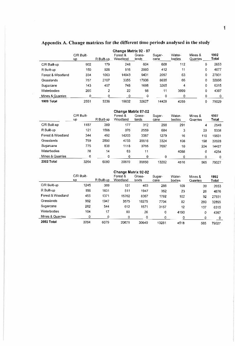
1

Appendix A. Change matrices for the different time periods analysed in the study

Change Matrix 92 - 97C/R Built- Forest & Grass- Sugar- Water- Mines & 1992

up R Built-up Woodland lands cane bodies Quarries Total

C/R Built-up 902 179 248 604 608 112 0 2653

R Built-up 150 928 516 2860 412 11 0 4877

Forest & Woodland 334 1063 14943 9431 2097 63 0 27931

Grasslands 757 2707 3355 17936 8035 66 0 32856

Sugarcane 143 457 748 1698 3265 4 0 6315

Waterbodies 265 2 22 98 11 3999 0 4397

Mines & Quarries 0 0 0 0 0 0 0 0

1999 Total 2551 5336 19832 32627 14428 4255 0 79029

Change Matrix 97-02C/R Built- Forest & Grass- Sugar- Water- Mines & 1997up R Built-up Woodland lands cane bodies Quarries Total

C/R Built-up 1187 280 177 312 298 291 4 2549

R Built-up 121 1566 376 2559 684 3 29 5338

Forest & Woodland 344 492 14203 3387 1279 16 110 19831

Grasslands 759 2890 4733 20616 3324 108 198 32628

Sugarcane 775 838 1118 3765 7697 10 224 14427

Waterbodies 78 14 63 11 4088 0 4254

Mines & Quarries 0 0 0 0 0 0 0 0

2002 Total 3264 6080 20670 30650 13282 4516 565 79027

Change Matrix 92-02C/R Built- Forest & Grass- Sugar- Water- Mines & 1992up R Built-up Woodland lands cane bodies Quarries Total

C/R Built-up 1245 369 151 463 286 109 30 2653R Built-up 186 1831 511 1947 352 23 26 4876Forest & Woodland 455 1371 15762 8367 1782 102 92 27931Grasslands 992 1947 3575 18275 7704 82 280 32855Sugarcane 282 544 612 1571 3157 12 137 6315Waterbodies 104 17 60 26 0 4190 0 4397Mines & Quarries 0 0 0 0 0 0 0 02002 Total 3264 6079 20671 30649 13281 4518 565 79027