AN ASSESSMENT OF THE VULNERABILITY OF GHANA’S COASTAL
83
AN ASSESSMENT OF THE VULNERABILITY OF GHANA’S COASTAL ARTISANAL FISHERY TO CLIMATE CHANGE By Sheila O. Minta Thesis Submitted in Partial Fulfilment of the Requirements for the Degree of Master of Science in International Fisheries Management Department of Aquatic Biosciences The Norwegian College of Fishery Science University of Tromsø Norway May 2003
Transcript of AN ASSESSMENT OF THE VULNERABILITY OF GHANA’S COASTAL
AN ASSESSMENT OF THE VULNERABILITY OF GHANA’S
COASTAL ARTISANAL FISHERY TO CLIMATE CHANGE
By
Sheila O. Minta
Thesis Submitted in Partial Fulfilment of the Requirements for the Degree of
Master of Science in International Fisheries Management
Department of Aquatic Biosciences
The Norwegian College of Fishery Science
University of Tromsø
Norway
May 2003

i
ACKNOWLEDGEMENTS
I am pleased to acknowledge the invaluable support of all who, in diverse ways have
contributed to the successful completion of this thesis. Special thanks go to Associate Professor
Jorge Santos for his excellent supervision, patience and constructive criticism, which moulded
the study into its best.
I am indebted to Mr William K. Agyemang Bonsu of the Environmental Protection Agency,
Ghana, for contributing to the Climate Change segment, and Mr Paul O. Onyango of Master
2002 (NFH-Tromsø) for sparing time to read and make useful suggestions. I am especially
grateful to Mr Sam Quaatey, Dr Kwame Koranteng and staff of the Marine Fisheries Research
Division, and to Frank of the Fisheries Research Library (FAO Regional Office, Accra) for
being so helpful with the collection of the secondary data and related literature. My heartfelt
gratitude goes to Mr Andrews Nkansah and Mr Minia of the Meteorological Services
Department, Ghana, for their assistance with the collection of the climatological data. The
financial support provided by the Government of Norway and SEMUT during data collection is
greatly appreciated.
Best compliments to you Mama, Iris, Olivia, Owuraku, Sisi Bea, Auntie Abena and all my
friends especially Ola, Sarah, Enoch and Mavis: your prayers and encouragement will not be
forgotten. To my husband Reuben, I say God richly bless you for your support and timely
arrival for the review and editing of this work.

ii
ABSTRACT
Considering the fact that nearly 25% of the Ghanaian people live in the coastal zone and about
10% depend on the coastal fishery for livelihood, it is likely that any changes in the production
of the fishery may impact on the socio-economic lives of the people. For the past four decades,
climatic conditions have been found to be changing in the country. This period coincided with
the conspicuous fluctuations in the landings of the most significant pelagic species exploited by
the canoe fleet. This study provides an assessment of the influence of precipitation and sea
surface temperature changes on yield and catch of Round Sardinella (Sardinella aurita),
anchovy (Engraulis encrasicholus), Flat Sardinella (S. maderensis) and Guinea Shrimp
(Parapenaeopsis atlantica). The abundance of these stocks is believed to be correlated with
upwelling and sea surface temperature conditions and a local manifestation of global scale
climatic changes is suspected to be taking place. It was hypothesized that climate as represented
by sea surface temperature (SST) and precipitation affects either catchability or the population
growth rate of each species. Forty years of climatological data (mean air temperature and
precipitation) were assessed; 38 and 33 years each of hydrological data (sea surface temperature
and salinity) were then used to investigate the possible relation between climatic changes and
species production. Forecasts of future climate scenarios were made, and stock dynamics were
simulated with an environmentally coupled dynamic surplus production model. Stock production
and, to a lower extent, catchability were found to be closely tied to climatological factors. Lower
catch rates of the Round Sardinella coincided with years of higher SST and the reverse was true
for the anchovy. For the shrimp and flat sardine, precipitation was found to have the most
substantial effect on production and total annual catchability. It was concluded that changes in
climate directly affect the productivity of the ecosystem as well as its catchability and most
importantly, the population growth rate of the species. For sustainable management of the
fishery resources, it is imperative that climatic and hydrological parameters be incorporated into
fishery management models.

iii
TABLE OF CONTENTS
1.0 Introduction
1.1 Rationale of the study…………………………………………………….…1
1.2 Objectives of the Study……………………………………………………...1
2.0 Description of the Fishery and Coastal Climate…………………………3
2.1 Natural Resources and Economy…………………………………………..3
2.1.1 The Fisheries Sub-sector……………………………………………………3
2.2 I Importance to Coastal Communities……………………………………….4
2.3 Biology of the Target Species of the Artisanal Fleet……………………….5
2.3.1 Sardinella aurita…………………………………………………………………...5
2.3.2 Sardinella maderensis…………………………………………………………….6
2.3.3 Scomber japonicus…………………………………………………………………7
2.3.4 Engraulis encrasicolus……………………………………………………….……7
2.3.5 Parapenaeopsis atlantica……………………………………………….….7
2.4 General Trends in the Production of the Fishery………………………….8
2.5 Climate and Hydrology……………………………………………………10
3.0 Literature Review and Background Theory……………………………12
3.1 Short Overview of Climate Change Activities in Ghana………………….12
3.2 The Coastal Climate and the Interaction With the Fishery………………..12
3.3 The Influence of Upwelling……………………………………………….14
3.4 SST Related Studies in the Gulf of Guinea Large Marine
Ecosystem (GOGLME)…………………………………………...……….16
3.5 Climate Models……………………………………………………………16
3.6 Hypotheses……………………………………………..………………….19
4.0 Materials and Methods……………………………………………..……19
4.1 Study Area…………………………………………………………………19
4.2 Data Required and Collected……………………………………………...20
4.3 Analysis Material………………………………………………………….20
4.4 Methodology………………………………………………………………20
4.4.1 Biological and Economic Production of Stock……………………………21

iv
4.4.2 Meteorological Data……………………………………………………….21
4.5 Fishery Models……………………………………………………………..21
4.5.1 The Fit of the Model………………………………………………………..23
4.5.2 Refinement of the Base Model…………………………………………….23
4.5.3 Selection of the Best Model………………………………………………..24
5.0 Results……………………………………………………………………..25
5.1 Trends in Climatic Parameters……………………………………………...25
5.1.1 Temperatures………………………………………………………….…….25
5.1.2 Salinity……………………………………………………………………....26
5.1.3 Precipitation………………………………………………………………....26
5.2 Correlations Among Climatic Variables…………………………………....27
5.3 Projected Climatic Scenarios……………………………………………..…31
5.4 Production Trends of the Canoe Fishery…………………………………..…33
5.5 Dynamic Production Model……………………………………………..…..34
.
6.0 Discussion…………………………………………………………………..43
6.1 Climatic Trends: Merely Local Changes?……………………………….…..43
6.2 Yield-Climate Interactions……………………………………………….….44
6.2.1 Anchovy……………………………………………………………………..45
6.2.2 Round Sardinella…………………………………………………………..…45
6.2.3 Flat Sardinella………………………………………………………….…….46
6.2.4 Guinea Shrimp and Chub Mackerel……………………………………….…46
6.3 Future Production…………………………………………………………….47
6.5 Limitations of the Study……………………………………………………..48
7.0 Conclusions………………………………………………………………….50
7.1 Lessons……………………………………………………………………….50
7.2 Recommendations………………………………………………………….…50

v
LIST OF FIGURES
Figure 2.1 Summary of Total Fish Production (1961-2001……………………....9
Figure 2.10 Distribution of Rainfall along the Coastal Zone of Ghana………...10
Figure 3.1 The Climatic Pathways Affecting the Abiotic
Environment of Fish……..…………………………………………….14
Figure 4.1 A Map of the Ghanaian Coastline Showing the Climate
and Fisheries Research Stations……………………………………….19
Figure 5.1 Trends in Mean Annual Air Temperature Along the
Coast of Ghana ……………………………………………………...25
Figure 5.2 Trends in SST Along the Coast of Ghana……………………….…26
Figure 5.3 Salinity Observations (1961 –2001)……………………………….26
Figure 5.4 Precipitation Trend (1961 – 2001………………………………….27
Figure 5.5 Variations of SST with MAT………………………………………..27
Figure 5.6 Variations of Coastal Precipitation With SST…………………….28
Figure 5.7 Variation of Precipitation with Mean Air Temperature………..28
Figure 5.8 Variations of Salinity with Changes in Precipitation…………...28
Figure 5.9 PCA Showing Correlation among Climatic
Variables (Log Transformed Species from 1970 to 2001 ……….29
Figure 5.10 PCA Showing Correlation among Climatic Variables
From 1970-2001 (Log Transformed series with
Year as covariate)…………………………………………………….29
Figure 5.11 RDA Showing Correlation Among Climatic Variables
(Log transformed Data With Previous Year’s
Temperature (MAT-1) as an Explanatory Variable……………..30
Figure 5.12 RDA showing Correlation among Climatic Variables
(Log transformed Data With Previous Year as Covariate
to Filter the Annual Trend…………………………………………..30
Figure 5.13 Projected Rainfall for the Coast of Ghana for Years
2001-2021 Based on Regression of Historical
Data (1961-2001)………………………………………………..….31
Figure 5.14 Projected SST Scenario for the Coast of Ghana for
years 2001-2021Based on Regression of Historical

vi
Data (1961-2001…………………………………………………….32
Figure 5.15 Projected Mean SST Scenario for the Coast of Ghana
for years 2001-2021 Based on Regression of Historical
Data (1961-2001)……………………………………………………32
Figure 5.16 Relative Significance of the Five Species in Terms of
Revenue to the Canoe Fleet (1980 – 2001………………………33
Figure 5.17 Relative Significance of the Five Species in Terms
of yield to the Canoe Fleet (1980 – 2001…………………………33
Figure 5.18 Best Fit of the CPUE –Based Model for the Anchovy
(1974 – 2001)…………………………………………………………36
Figure 5.19 Best Fit of the r–Based Model for the Anchovy
(1974 – 2001………………………………………………………….36
Figure 5.20 Catch and Biomass Curve of the r – Based Model
for the Anchovy……………………………………………………….36
Figure 5.21 SST-dependent Fit for the Round Sardinella in the
CPUE –Based Model (1973-2001………………………………....37
Figure 5.22 Best Fit for the Round Sardinella in the r-based
Model (1973 – 2001)………………………………………………..37
Figure 5.23 Catch and Biomass Curves of the r – Based Model
for the Round Sardinella…………………………………………….37
Figure 5.24 Best Fit of the r–Based Model for the Guinea
Shrimp (1980– 2001)………………………………………………….38
Figure 5.25 Best Fit of the CPUE –Based Model for the Guinea
Shrimp (1980– 2001)………………………………………………….39
Figure 5.26 Best Fit of the Precipitation Dependent r–Based
Model for the Flat Sardinella (1972-2001)………………………39
Figure 5.27 Catch and Biomass Curves of the r – Based Model for
the Flat Sardinella………………………………………………….39
Figure 5.31 Best Fit of the CPUE- Based Model For the Chub
Mackerel (1970 –2001)……………………………………………….41
Figure 5.32 Best Fit of the r-Based Model For the Chub
Mackerel (1970 –2001)……………………………………………….41
Figure 5.33 Catch and Biomass Curves of the r-based

vii
Model for the Chub mackerel (1972-2001)………………………..41
List of Plates
Plate 1 Sardinella aurita (Round Sardinella)……………………………....6
Plate 2 Sardinella maderensis (Flat Sardinella)……………….…………..6
Plate 3 Scomber Japonicus (Chub Mackerel)….……………………….…..7
Plate 4 Engraulis encrasicolus (Anchovy)…….……..………………………7
Plate 5 Parapenaeopsis atlantica (Guinea Shrimp)…..………….…………8
LIST OF TABLES
Table 2.1 Fleets exploiting the Coastal Fishery in Ghana……………..…..4
Table 2.2 Trend of Variation in the Canoe Fleet (1969 – 2001)……….…9
Table 5.1 Production Model Estimates for the Anchovy
(1974 –2001)………………………………………………………..34
Table 5.2 Production Model Estimates for the Round
Sardine (1973 –2001) ……………………………………………34
Table 5.2 Production Model Estimates for the Flat
Sardine (1972 –2001)……………………………………………..35

viii
LIST OF APPENDICES.
Appendix 1 Summary of Annual Variations in Climatic variables
Source MSD Data base, MFRD…………………………..………..…59
Appendix 2A Trends in Maximum and Minimum Mean Air Temperature………60
Appendix 2B Autocorrelation Analysis: Mean Air Temperature…………….…...60
Appendix3A Autocorrelation Analysis: SST………………………………………...61
Appendix3B Comparism of SST Values used by Anakwah and Santos,
2002 and Minta, 2003,1975 – 1999……………………………..…....61
Appendix 4A Autocorrelation Analysis: Total Coastal Precipitation……,.……..62
Appendix 4B Fluctuations in Historic MAT………………………………...…..,….62
Appendix 5A Fluctuations of Historic SST About the Mean …………………......63
Appendix 5B Fluctuations of Historic Salinity About the Mean…...…………..….63
Appendix 5C Fluctuations of Historic Precipitation About the Mean…………….63
Appendix 6A Seasonal Variation of MAT (1961 - 2001)……………………….....64
Appendix 6B Seasonal Variation of Precipitation (1961 - 2001)…………….…...64
Appendix 6C Seasonal Variation of Salinity (1968 – 2001)……………..……..….64
Appendix7A Seasonal Variation of Maximum and Minimum
Temperature (1960 – 2001)……………………………………………65
Appendix7B Results of Correlation Analysis for Climatic variables
Measured Along the Coast of Ghana……………………………..…65
Appendix 8A Regression Statistics for precipitation Trend along
the Coast of Ghana………………………………………………….….66
Appendix 8B Regression Statistics for SST Trend Along
the Coast of Ghana…………………………………………………..…66
Appendix 9 Annual Production of the Major Marine Stocks
in Ghana………………………………………………………………...67
Appendix 10A Fluctuations in Landings of Round Sardine in
Relation to SST Deviations from the Mean…………………………..…68
Appendix 10B Fluctuations in Landings of Flat Sardine in
Relation to SST Deviations from the Mean………………………….68
Appendix 10C Fluctuations in Landings of Anchovy in Relation.
to SST Deviations from the Mean……………………………………68

ix
Appendix 11A Fluctuations in Landings of Chub Mackerel in Relation
to SST Deviations from the Mean…………………………..………...……...69
Appendix 11B Fluctuations in Landings of Guinea Shrimp in Relation
to SST Deviations from the Mean……………………………..…………...….69
Appendix 11C Model Estimates for the Chub mackerel (1972 – 2001)……….….69
Appendix 12A Model Estimates for the Guinea Shrimp (1980 – 2001)…………...70 Appendix 12B variation of prices for the Main Stocks harvested by
The Ghanaian Canoe Fleet………………………………….……..…70
Appendix 13 Contribution of the Small Pelagics and Guinea Shrimp
to Annual Revenue of the Canoe Fishery……………………….…..71
Appendix 14 Calculation of the MSY for Anchovy using annual
Appendix 15 Calculation of the MSY for Round Sardine Using
Annual Values Estimated by Incorporation of SST ………….…...73
1
1.0 INTRODUCTION
Increasing fishing effort on marine stocks has major impacts on the short-term
dynamics and sustainability of the fish populations (Bakun, 1993; King 1995).
Availability and distribution of the short- lived small pelagics, the tuneids and shrimp,
have also been related to environmental changes, particularly variations in the ocean
climate.
Precipitation, river-runoff and salinity have been found to be vital determinants of
penaeid shrimp abundance (Condrey and Fuller, 1992). Sea surface temperature
(SST) influences the distribution and availability of tuneids (Bages and Fonteneau,
1980; Sharp, 1992) and the seasonality and productivity of the fisheries such as those
in the Gulf of Guinea upwelling areas (McGlade et al. 2002). However, fisheries
management policies and practices are usually based on catch effort dynamics with
little consideration of the ecosystem variations. Thus, the local effects of a change in
global climatic conditions are likely to go unnoticed and would affect the most
heavily exploited stocks in developing countries such as Ghana which have coastal
communities with a high dependence on them (Glantz, 1992; IPCC, 2001).
1.1 Rationale of This Study
The exact cause-effect relationships between climate and stock variability are poorly
understood because the relationship is difficult to define. Some studies relating the
productivity to environmental factors have been undertaken for the Gulf of Guinea.
Koranteng and McGlade (2002), Hardman-Mountford and McGlade (2002) Demarcq
and Aman (2002) and Arfi et al. (2002) analysed how the dynamics of commercial
stocks relates to the patterns in SST. The seasonal nature of the fishery and its close
association to upwelling and SST has been confirmed. This could, however, be
explained either in terms of species movement/migration to the fishing area occurring
along a climatic gradient or more favourable conditions for population growth or
both. Since little has been done to clarify this relationship, an attempt is made in the
present study to assess which of these mechanisms is more applicable for the
Ghanaian fishery.

2
1.2 Objectives of the Study
The ultimate objective of this thesis is to investigate the relationship between climate
and the catch per unit effort (CPUE). Pertinent questions to ask in this regard would
be:
• What have been the trends in landings of the main commercial fish stocks for the
past 30 – 40 years?
• What have been the past climatic conditions?
• What historical relationships have been or can be established between the climate
variability and fish yield?
• Which models have been used in similar studies and to what extent can they be
used to predict future marine yields in Ghana?
It is expected that the answers to these questions would help to achieve the following
specific objectives:
To assess the potential impact of climate change on the coastal fishery using existing
historical climate data,
To forecast the dynamics of the main commercial stocks for 5- 20 years ahead in the
absence of increases in fishing effort,
To develop possible adaptation options that can be integrated into management, and
conservation of the living aquatic resources, and
To provide a basis for country –wide studies that can produce an input to Ghana’s
Second National Communication under the United Nations Framework
Convention on Climate Change (UNFCCC).
3
2.0 DESCRIPTION OF THE FISHERY AND COASTAL CLIMATE
The Republic of Ghana is situated in West Africa along the Greenwich meridian
between latitudes 4.5 o N, 11.5 o N and longitude 3.5o W, 1.3o E. To the East, West
and North are the Republic of Togo, La Côte d’Ivoire and Burkina Faso respectively.
The total area of 238,540 km2 is washed to the South by the Gulf of Guinea. The
population is estimated at 19.7 million and growing at a rate of about 3% per annum,
with about 10% being almost entirely dependent on the marine fishery for livelihood
(Quaatey, 1996; Republic of Ghana, 2000).
2.1 Natural Resources and the Economy
The vast array of renewable and non-renewable resources includes precious minerals
(gold, diamond, copper and manganese), forests, fisheries, game and wildlife. Over
50% of the GDP is provided by the agricultural sector, which includes crops, Forestry
and Fisheries. The main crops cultivated and consumed locally are rice, coffee,
cassava, peanuts, corn, sheanuts while those cultivated for export are cocoa and
coffee. Other exports include gold, timber, bauxite, aluminium and tuna (Isaka et al.
2002).
2.1.1 The Fisheries Sub-sector
Though contributing only about 3% to national GDP and 5% of Agricultural GDP,
Fisheries provide about 65% of the animal protein intake of the entire populace. Like
in all tropical countries, fish species diversity is high with about 447 in the marine
waters, 227 in the inland waters and 19 species produced in aquaculture. Aquaculture
activities are still yet to obtain a sound footing and the inland fisheries constitute only
16% of the total annual production. The marine fishery is, thus, the mainstay of the
sub-sector and has been a significant non-traditional export since the introduction of
the Economic Recovery Program in 1984 (Quaatey, 1996). The area of operation for
this is the Eastern Central Atlantic Fishing Area (CECAF), which spans most
countries in the sub-region. The coastline is 528 km long with an Exclusive Economic
Zone (EEZ) of over 218,000 km2 and a continental shelf of 23,700 km2. With most of
the country’s major rivers emptying into the sea, Ghana’s coastal fishery is the 4th
most productive of 36 countries in the Atlantic. Three main fleets exploit it: Artisanal
(over 70% of total marine catch), Inshore or Semi- industrial and the Deep-Sea or

4
Industrial, which can be categorised into the large trawlers and the Tuna vessels
(Table 2.1).
Table 2.1 Fleets Exploiting the Coastal Fishery in Ghana (Anakwah and Santos
2002, Isaka et al. 2002).
Fleet Vessel Type/Size Target Species Gear Type
Artisanal Canoe, up to 8 m Anchovy, Sardines, Mackerels,
Guinea Shrimp, Burrito
Drift Nets, Purse Seine
Semi -
Industrial
Small Boats, 8-37 m Anchovy, Sardines, Mackerels,
Burrito, Other Demersals
Purse Seine, Trawls
Large Steel Vessels
over 35 m
Sardines, Chub Mackerel, Horse
Mackerel, Shrimp, Cephalopods
Trawls Industrial:
Large
Trawlers
Tuna
Large Vessels over
30 m
Skipjack, Yellowfin, Bigeye Pole and Line, Long
Lines, Purse Seine, Fish
Aggregation Devices
2.2 Importance to Coastal Communities
The coastal zone is characterised by rivers, lagoons and marshes connecting to the
ocean. The major rivers are flooded during the rainy season and empty into the sea.
Though it forms only about 7% of the nation’s land area, the coastal area houses most
of the major cities and towns: Accra (the capital), Tema (main harbour and industrial
city,) Sekondi-Takoradi (Harbour city), Cape Coast, Elmina and Ada (tourist centres).
It is, therefore not surprising that about a quarter of the populace (about 21 districts in
4 of the country’s 10 regions) reside here. It is also home to numerous productive
lagoons. Majority of the people lives in rural communities where the major
occupation is fishing and they are organised into about 200 fishing villages and nearly
300 landing beaches. Thus there is a high dependence on fisheries (currently open
access) for food and livelihood. Employment has been created for several thousands
of people in the industry such as processors, traders, exporters, boatbuilders and the
middlemen who supply communities in the hinterlands.

5
The tuna fleet is the most important foreign exchange earner followed by the
industrial shrimpers but as far as fish yield, employment and livelihood are concerned,
the Artisanal fleet plays a dominant role. The stocks exploited are the Round Sardine,
Flat Sardine, Anchovy, Chub Mackerel and Frigate mackerel. The first four are
usually used to characterise the canoe fleet (small pelagics) since they are the most
common and constitute over 60% of the landings. Others are the Guinea shrimp, Sea
Breams, and Burrito. The tunas are mostly Yellowfin, Bigeye and Skipjack (Quaatey,
2002).
The Ghanaian canoe fleet has for a long time been a good example of how African
indigenous fisheries can successfully develop to a modern stage. Fishing is done by
the fishermen way beyond the national boundaries in spite of many economic
difficulties. The fishing methods and gear that they have introduced have strongly
influenced the kind of fisheries found there for example, in Sierra Leone and Guinea
(Dykhuizen and Zei, 1970).
2.3 Biology of the Target Species of the Artisanal Fleet
Most of these fish stocks are shared along the subregion and in the fishing area and
are believed to follow a migratory pattern along upwelling areas. However, the most
noticeable aggregation areas are the Ghana-Ivorian shore (Dykhuizen and Zei, 1970).
.
2.3.1 Sardinella aurita
Commonly called the Round Sardinella, this species belongs to the order
Clupeiformes of the family Clupeidae and the class Actinopterygii (Plate 1). It is
locally called ‘Eban’ or ‘Kankama’. It is usually found in marine pelagic waters of 0-
350m depths especially in West Africa. It is distributed in subtropical a climate
(46°N-36°S) that is in the Black and Mediterranean Seas, in the Eastern Atlantic as
well as in the Western Atlantic. Spawning occurs during the upwelling seasons. It is a
highly schooling fish usually associated with the inshore shelf area and having a
diurnal migratory feeding pattern. Its typical diet is mainly composed of zooplankton
and copepods. It is classified by the FAO as highly commercial and used locally for
food as well as for live-bait in tuna fishing in CECAF. The size distribution in Ghana
has been estimated as 5-15cm for the beach seine and 18cm for the ring net (Anakwah
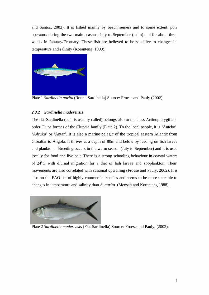
6
and Santos, 2002). It is fished mainly by beach seiners and to some extent, poli
operators during the two main seasons, July to September (main) and for about three
weeks in January/February. These fish are believed to be sensitive to changes in
temperature and salinity (Koranteng, 1999).
Plate 1 Sardinella aurita (Round Sardinella) Source: Froese and Pauly (2002)
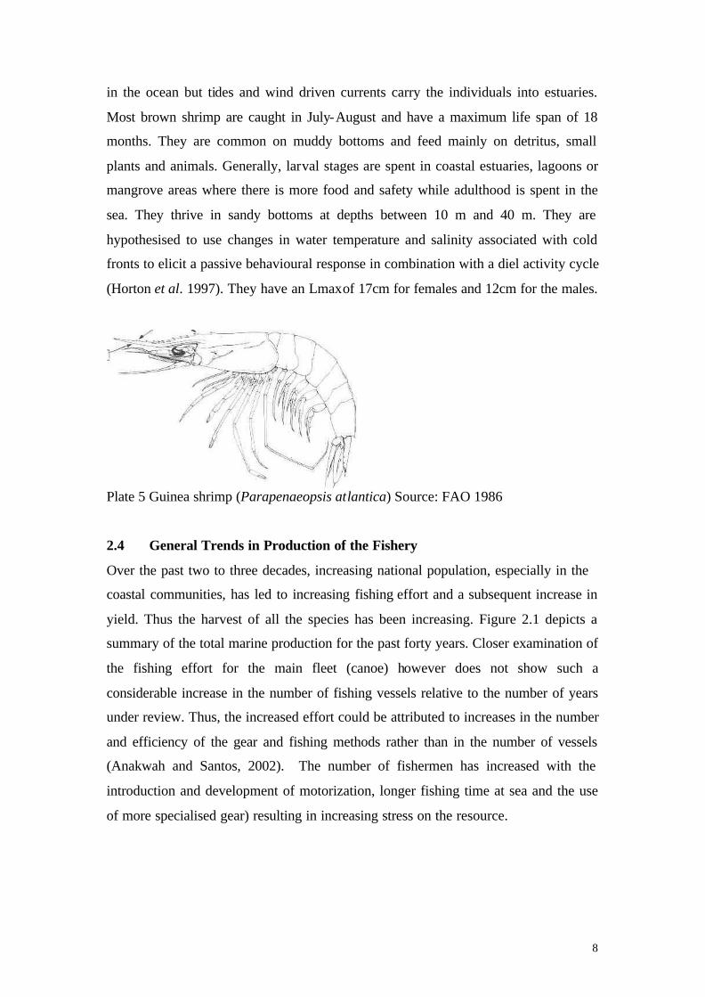
2.3.2 Sardinella maderensis
The flat Sardinella (as it is usually called) belongs also to the class Actinopterygii and
order Clupeiformes of the Clupeid family (Plate 2). To the local people, it is ‘Antebo’,
‘Adruku’ or ‘Antar’. It is also a marine pelagic of the tropical eastern Atlantic from
Gibraltar to Angola. It thrives at a depth of 80m and below by feeding on fish larvae
and plankton. Breeding occurs in the warm season (July to September) and it is used
locally for food and live bait. There is a strong schooling behaviour in coastal waters
of 24oC with diurnal migration for a diet of fish larvae and zooplankton. Their
movements are also correlated with seasonal upwelling (Froese and Pauly, 2002). It is
also on the FAO list of highly commercial species and seems to be more tolerable to
changes in temperature and salinity than S. aurita (Mensah and Koranteng 1988).
Plate 2 Sardinella maderensis (Flat Sardinella) Source: Froese and Pauly, (2002).

7
2.3.3 Scomber japonicus
This is a marine pelagic commonly called the Chub Mackerel. It occurs in waters up
to 300m deep in subtropical climates (60°N-55°S). It is locally referred to as ‘Saman’
and belongs to the family Scombridae, order Perciformes and Class Actinopterygii
(Plate 3). It shows strong schooling behaviour even with other species and also
migrates diurnally to feed mainly on copepods. It is also reported as one of the stocks
that could be affected directly or indirectly by climate change (Rothschild, 1996).
Plate 3 Scomber japonicus (Chub Mackerel) Source: Froese and Pauly (2002)
2.3.4 Engraulis encrasicolus
The anchovy is another marine pelagic found in the eastern north and central Atlantic
between 62°N and 19°S. It also occurs in brackish water. It is locally called ‘Bornu
or ‘Keta school boys’. It belongs to the family Engraulidae, order Clupeiformes and
class Actinopterygii (Plate 4). Breeding occurs during the warm months. It is
migratory and schooling occurs in saline waters. The diet is mainly composed of
plankton. They can thrive in salinities of 5-41ppt and in certain regions, migrate into
lagoons, estuaries and lakes during spawning. It is also classified by the FAO as
highly commercial.
Plate 4 Engraulis encrasicolus (Anchovy) Source: Froese and Pauly (2002)
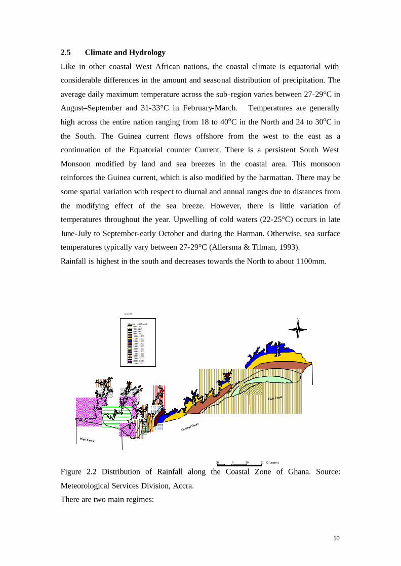
2.3.5 Parapeneospsis atlantica
This species of shrimp is commonly called the Guinea shrimp or the Brown Shrimp
by virtue of its brownish greyish colour. However, it turns a beautiful red after
cooking and is the main species caught off the West African coast. Spawning occurs
8
in the ocean but tides and wind driven currents carry the individuals into estuaries.
Most brown shrimp are caught in July-August and have a maximum life span of 18
months. They are common on muddy bottoms and feed mainly on detritus, small
plants and animals. Generally, larval stages are spent in coastal estuaries, lagoons or
mangrove areas where there is more food and safety while adulthood is spent in the
sea. They thrive in sandy bottoms at depths between 10 m and 40 m. They are
hypothesised to use changes in water temperature and salinity associated with cold
fronts to elicit a passive behavioural response in combination with a diel activity cycle
(Horton et al. 1997). They have an Lmax of 17cm for females and 12cm for the males.
Plate 5 Guinea shrimp (Parapenaeopsis atlantica) Source: FAO 1986
2.4 General Trends in Production of the Fishery
Over the past two to three decades, increasing national population, especially in the
coastal communities, has led to increasing fishing effort and a subsequent increase in
yield. Thus the harvest of all the species has been increasing. Figure 2.1 depicts a
summary of the total marine production for the past forty years. Closer examination of
the fishing effort for the main fleet (canoe) however does not show such a
considerable increase in the number of fishing vessels relative to the number of years
under review. Thus, the increased effort could be attributed to increases in the number
and efficiency of the gear and fishing methods rather than in the number of vessels
(Anakwah and Santos, 2002). The number of fishermen has increased with the
introduction and development of motorization, longer fishing time at sea and the use
of more specialised gear) resulting in increasing stress on the resource.

9
Figure 2.1 Summary of Total Marine Fish Production (1961-2001) Source: MFRD,
Ghana.
Table 2.2 Trend of Variation in the Canoe Fleet -1969-2001. Source, Anakwah and
Santos (2002), MFRD (2002). *Unavailable data
Year Canoes Outboard Motors %
Motorization
1969 8728 * *
1973 8238 * *
1977 8742 * *
1981 6983 3698 53.3
1986 8214 4250 51.7
1989 8052 4631 57.5
1992 8688 4262 49.1
1995 8641 5076 58.7
1997 8610 5139 61.2
1999 8895 * *
2001 9981 * *
The fishery has exhibited high fluctuations, especially the S. aurita that constitutes
over 50% of the annual landings. Its amount and availability seem to determine the
annual production of the fishery. There are corresponding yearly fluctuations in catch
and catch per unit effort (CPUE). Unusually high catches were recorded in 1972 due
to availability of the fish. However, a poor landing was recorded in the ensuing years
attributed mainly to overfishing and anomalous climatic conditions (Koranteng,
1991). Generally, the small pelagics are believed to be overexploited in spite of the
recent increases in landings (Mensah and Quaatey, 2002).
Trend in Total Marine Fish Production
0
100000
200000
300000
400000
500000
1961
1965
1969
1973
1977
1981
1985
1989
1993
1997
2001
Year
Cat
ch (m
etri
c to
nnes
)
10
2.5 Climate and Hydrology
Like in other coastal West African nations, the coastal climate is equatorial with
considerable differences in the amount and seasonal distribution of precipitation. The
average daily maximum temperature across the sub-region varies between 27-29°C in
August–September and 31-33°C in February-March. Temperatures are generally
high across the entire nation ranging from 18 to 40oC in the North and 24 to 30oC in
the South. The Guinea current flows offshore from the west to the east as a
continuation of the Equatorial counter Current. There is a persistent South West
Monsoon modified by land and sea breezes in the coastal area. This monsoon
reinforces the Guinea current, which is also modified by the harmattan. There may be
some spatial variation with respect to diurnal and annual ranges due to distances from
the modifying effect of the sea breeze. However, there is little variation of
temperatures throughout the year. Upwelling of cold waters (22-25°C) occurs in late
June-July to September-early October and during the Harman. Otherwise, sea surface
temperatures typically vary between 27-29°C (Allersma & Tilman, 1993).
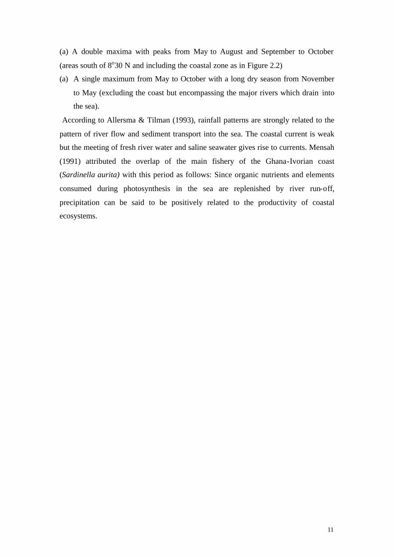
Rainfall is highest in the south and decreases towards the North to about 1100mm.
Figure 2.2 Distribution of Rainfall along the Coastal Zone of Ghana. Source:
Meteorological Services Division, Accra.
There are two main regimes:
East Coast
Central Coast
West Coast
Mean Annua l Rain fa ll600 - 70 0700 - 80 0800 - 90 0900 - 10 001000 - 1 1001100 - 1 2001200 - 1 3001300 - 1 4001400 - 1 5001500 - 1 6001600 - 1 7001700 - 1 8001800 - 1 9001900 - 2 0002000- 2 1002100 - 2 200
LEGEND
N
30 0 30 60 Kilometers
11
(a) A double maxima with peaks from May to August and September to October
(areas south of 8o30 N and including the coastal zone as in Figure 2.2)
(a) A single maximum from May to October with a long dry season from November
to May (excluding the coast but encompassing the major rivers which drain into
the sea).
According to Allersma & Tilman (1993), rainfall patterns are strongly related to the
pattern of river flow and sediment transport into the sea. The coastal current is weak
but the meeting of fresh river water and saline seawater gives rise to currents. Mensah
(1991) attributed the overlap of the main fishery of the Ghana-Ivorian coast
(Sardinella aurita) with this period as follows: Since organic nutrients and elements
consumed during photosynthesis in the sea are replenished by river run-off,
precipitation can be said to be positively related to the productivity of coastal
ecosystems.

12
3.0 LITERATURE REVIEW AND BACKGROUND THEORY
3.1 Short Overview of Climate Change Activities in Ghana
After ratifying the United Nations Framework Convention on Climate Change
(UNFCCC) on December 5, 1995 a number of activities have been carried out in line
with Ghana’s commitment to the UNFCCC. These include the preparation of an
inventory of greenhouse gases (GHGs), impact assessments for water resources,
agriculture, and the coastal zone. Others are the possible abatement options in the
forestry and energy sectors and the development of future national scenarios. The
occurrence of climate change was observed in the form of sea level rise, coastal
erosion and a general increase in GHG emissions. A warming rate of 0.2oC per
decade and 5.4% decrease in rainfall was observed for the whole nation (Republic of
Ghana, 2000). Using General circulation Models (GCMs), scenarios were developed
up to 2100 for nationa l air temperatures and precipitation. However, the Fisheries
sub-sector was not covered in these assessments and there are currently no
predictions for the sea surface temperature (Republic of Ghana, 2000).
3.2 The Coastal Climate and Its Interaction with the Fishery
The Guinea current, blows from Guinea-Bissau in the north of the sub-region to
Angola in the South, and has a weak link with local winds. According to Quaatey
(1996), seasonality is exhibited on the coastal waters, which are dominated by a
seasonal upwelling occurring twice a year. At this time, water temperatures typically
drop below 25oC. The major upwelling lasts about three months (late June or early
July to late September or early October). The minor one occurs in January, February
or March for not more than three weeks. The only exception to this trend was in 1986
when it lasted for 10weeks.
The two seasons are characterised by decreases in SST, increases in salinity and
decrease in dissolved oxygen. The mixing of cold and nutrient rich lower layers with
water surface layers enhances productivity. The increased population of phyto and
zooplankton leads to increased production of higher taxa, particularly fish. For the rest
of the year, a strong thermocline exists which fluctuates in depth between 10 and
40m. The coastal climate has been linked to the abundance and availability of pelagic
13
stocks by several authors including Mensah and Koranteng, 1988, Mensah, 1991,
FAO, 1997.
Oceans are an integral and responsive component of the climate system with
important physical and biogeochemical feedback to the climate. The atmosphere and
oceans store and exchange energy in the form of heat and moisture, with the oceans
being the largest reservoir of moisture. They are more effective heat absorbers than
land and ice surfaces and better heat reservoirs than land. Hence, oceans can alter
atmospheric conditions and the weather. Kawasaki (1992) observed that increased
concentration of greenhouse gases (Carbon Dioxide, Water Vapour, Methane, Nitrous
Oxide and Chlorofluorocarbons) and, hence, global warming could increase sea
surface temperatures or distort the rainfall pattern. It could also intensify wind stress
on the sea with a resultant acceleration in coastal upwelling. Climatic factors affect
the biotic and abiotic elements that influence the numbers and distribution of fish
species. The abiotic elements include water temperature, salinity, nutrients, sea level
and current conditions while biotic factors include food availability and presence and
species composition of predators and competitors. Water temperatures can directly
affect spawning and survival of juveniles as well as fish growth (Laevastu and Hayes,
1981).
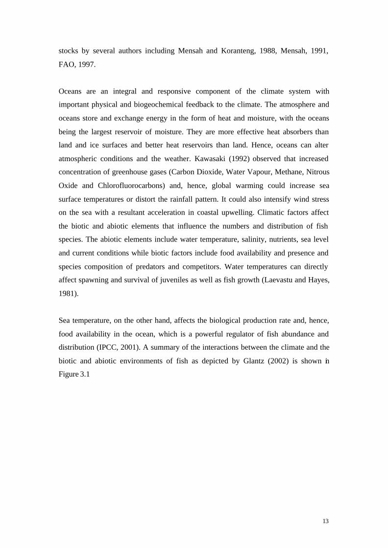
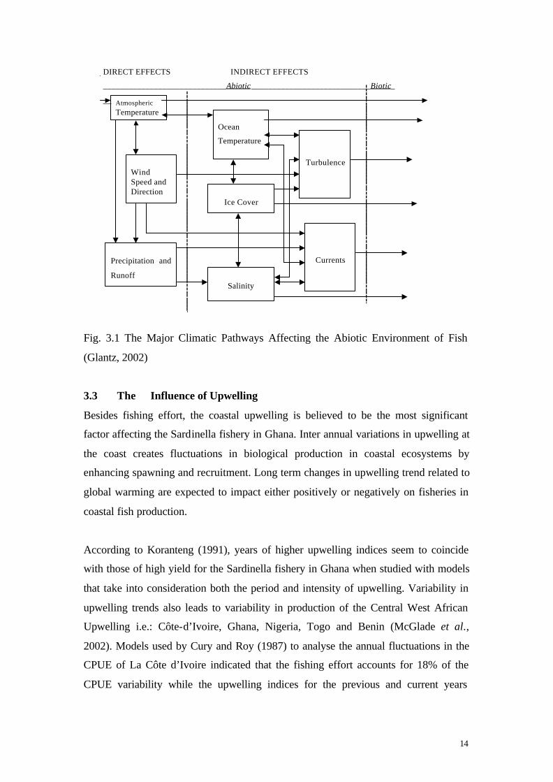
Sea temperature, on the other hand, affects the biological production rate and, hence,
food availability in the ocean, which is a powerful regulator of fish abundance and
distribution (IPCC, 2001). A summary of the interactions between the climate and the
biotic and abiotic environments of fish as depicted by Glantz (2002) is shown in
Figure 3.1
14
Fig. 3.1 The Major Climatic Pathways Affecting the Abiotic Environment of Fish
(Glantz, 2002)
3.3 The Influence of Upwelling
Besides fishing effort, the coastal upwelling is believed to be the most significant
factor affecting the Sardinella fishery in Ghana. Inter annual variations in upwelling at
the coast creates fluctuations in biological production in coastal ecosystems by
enhancing spawning and recruitment. Long term changes in upwelling trend related to
global warming are expected to impact either positively or negatively on fisheries in
coastal fish production.
According to Koranteng (1991), years of higher upwelling indices seem to coincide
with those of high yield for the Sardinella fishery in Ghana when studied with models
that take into consideration both the period and intensity of upwelling. Variability in
upwelling trends also leads to variability in production of the Central West African
Upwelling i.e.: Côte-d’Ivoire, Ghana, Nigeria, Togo and Benin (McGlade et al.,
2002). Models used by Cury and Roy (1987) to analyse the annual fluctuations in the
CPUE of La Côte d’Ivoire indicated that the fishing effort accounts for 18% of the
CPUE variability while the upwelling indices for the previous and current years
DIRECT EFFECTS INDIRECT EFFECTS
_____________________________Abiotic____________________________Biotic_
_____ _AtmosphericTemperature
WindSpeed andDirection
Precipitation and
Runoff
Ocean
Temperature
Ice Cover
Salinity
Turbulence
Currents

15
accounted for 40%. The seasonal coastal upwelling periodically modifies the physico-
chemical parameters of the water masses and controls the biology of the subsystem.
Mensah (1991) observed a correlation between the dominant rainfall pattern, river
discharge and sediment transportation and zooplankton production. This rainfall
pattern always precedes the major upwelling, which produces outbursts of fish yield.
The upwelling seems to provide a favourable habitat and occurs spontaneously with
spawning near Cape Three Points (Roy, 1996). Though the dynamics of upwelling
systems appear to be different and not clearly defined, wind stress is believed to be an
important cause. Binet (1997) noted that Sardinella catches are related to along-shore
wind stress of the year except during the early months of larval life. Increased wind
stress induces enrichment favourable for larval survival except immediately after
hatching when turbulence and offshore advection induce adverse effects. It would
therefore be expected that warmer years with higher sea surface temperatures would
be characterised by increased number of eddies at Cape Three Points. With spawning
occurring in this region, the enlarged turbulent structures would enable the survival of
a large number of larvae.
Verstraete (1983) also detected a linkage between the upwelling event, mean sea level
and dynamic height of the sea. Just before the start of the major upwelling, there is a
simultaneous drop in mean sea level and dynamic height at Tema and Takoradi. It has
been suggested that the changes in the Sardinella populations in the last decade could
have been induced by long-term environmental fluctuations (Roy, 1993). According
to Bakun (1993), the dramatic changes in the pelagic fish yield in the Gulf of Guinea
could either be a result of global scale climatic effects that could lead to
intensification of coastal upwelling, or of teleconnections to the Pacific El Nino
Southern Oscillation (ENSO) system. However, each of these causes suggests
differing scenarios for the future of the local fishery and would require further
research for adequate scientific basis to choose between them.

16
3.4 SST- Related Studies in the Gulf of Guinea Large Marine Ecosystem
(GOGLME) Fishery
In his analysis of the ocean environment, Mendelssohn (1988) observed that salinity,
SST and wind (North-South) have a strong long-term memory component. He
suggested that SST might even be an infinite variance series since it seems to reflect
the essential processes that affect fish dynamics. However, Aman (1999) pointed out
that measurements of only SST do not adequately describe the rise of the thermocline
during the upwelling season. Nevertheless, SST is often used to quantify the
upwelling.
Observations of remotely sensed SST data and the mean percentage of cloud
contamination showed a close relation between atmospheric and oceanographic
processes, which are subject to high variability (Hardman-Mountford and McGlade
2002). This was reflected in the seasonal feature of the fishery and suggests the
possib le presence of a 3-5year El Nino cycle and to some extent, the forcing of SST
by global scale climate interactions.
3.5 Climate Models
General Circulation Models or Global Climate Models (GCMs) are computer
simulations of the earth’s surface and atmosphere. The latter is divided into grids.
Fundamental equations describing the conservation of mass, energy and momentum,
for each grid are solved. They numerically simulate changes in climate as a result of
slow changes in some boundary conditions (such as the solar constant) or physical
parameters (such as the greenhouse gas concentration). They can be run long enough
to learn about the climate in a statistical sense that is, the means and variability and to
predict future climatic condition (Kattenberg et al., 1995; Spencer, 2001).
Several types of GCM are used differently to model the different components of the
climate: 3DAtmospheric models (AGCM), 3D Ocean models (OGCM), Atmospheric
chemistry models, Regional Climate Models, Carbon cycle models and coupled
Atmosphere Ocean models (AGCM+OGCM). The most common are the AOGCMs
that can be used for the prediction and rate of change of future climate. They are also
used to study the variability and physical processes of the coupled climate system as
17
in this study. For example, an accurate coupling could be used to simulate the ENSO
(Kerr, 1984; Berger et al. 1989).
Generally, simulating interannual variability in the presence of an annually varying
sun continues to be a difficult problem. Although some models reproduce interannual
SST variability and others reproduce the annual cycle, reproduction of the full
spectrum of variability remains elusive. (Since the annual cycle is an average over all
the variability present in the system [i.e., the average of all Januarys, Februarys, etc.],
the annual cycle is not independent of interannual variability.)
The basic problem with these models is that is that the processes that determine the
annual cycle appear to be different from the processes that determine the interannual
variability. In particular, interannual SST variability in the Pacific is believed to be
dependent on wind-driven thermocline variations with heat fluxes at the surface
acting mainly to damp the interannual perturbations. Annual variations of SST depend
critically on heat flux variations at the surface and therefore depend in an essential
way on radiative and cloud feedback. The presence of low-level stratus clouds exhibit
a positive feedback to SST at low tropical SSTs and therefore induce a special
sensitivity. In existing GCMs, these are poorly dealt with. Also, vertical mixing is
poorly represented in the current generation OGCMs used for tropical studies is
believed to have affected the simulated SST in the eastern equatorial Pacific, where
the changes in the wind stress play a key role in causing annual SST variability
(Sloane and Tesche, 1991; Houghton, 1997; Schnur 2002).
In the literature reviewed so far, no SST predictions for the Gulf of Guinea by these
models were obtained. Thus, in the present study, an attempt was made to extract
patterns from historical climate data and to forecast the main trends for the next 20
years. Uncertainty of the future trends was suggested by the utilization of confidence
intervals.
3.6 Hypotheses
It is imperative to investigate further the effects of other climatic components on the
other small pelagics and to forecast the possible effects on future productivity. Based
on the current review and the observations of Anakwah and Santos (2002) showing

18
the SST to have a positive effect on the CPUE of the anchovy and a negative one on
the round sardine, we could hypothesise that:
(i) The climatic conditions affect the distribution of the fish thereby affecting
their catchability, or
(ii) The climatic conditions affect othe r aspects of the biology such as the growth
rate of the population
The present study will investigate which of these two hypotheses is more applicable
to the fish populations and would be useful in an ecosystem-based approach to
management. The analytical method utilized to test the hypotheses was a fishery
model, which could account for the additional effects of climatic variables. Different
climatic variables were included separately and the model adopted to reflect changes
in the catchability (and thus distribution) or in the rate of population growth. The
fishery resources considered were those exploited by the canoe fleet and considered
most important)
.
.
19
4.0 MATERIALS AND METHODS
4.1 Study Area
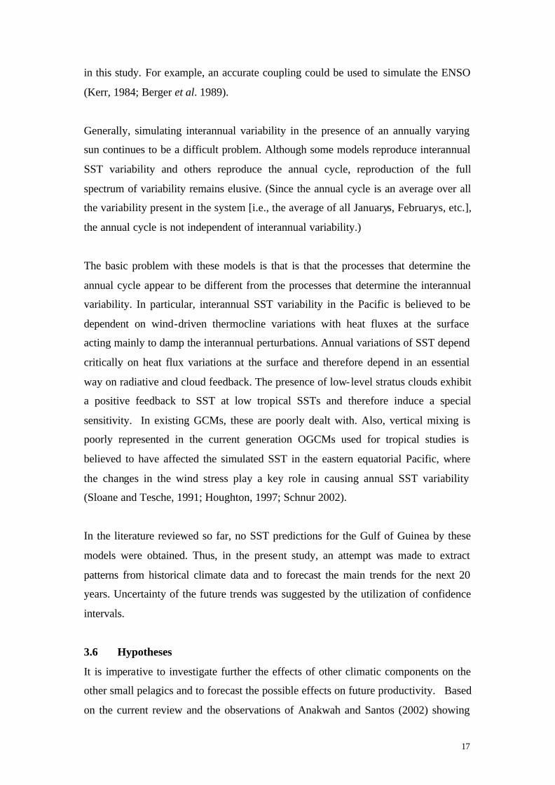
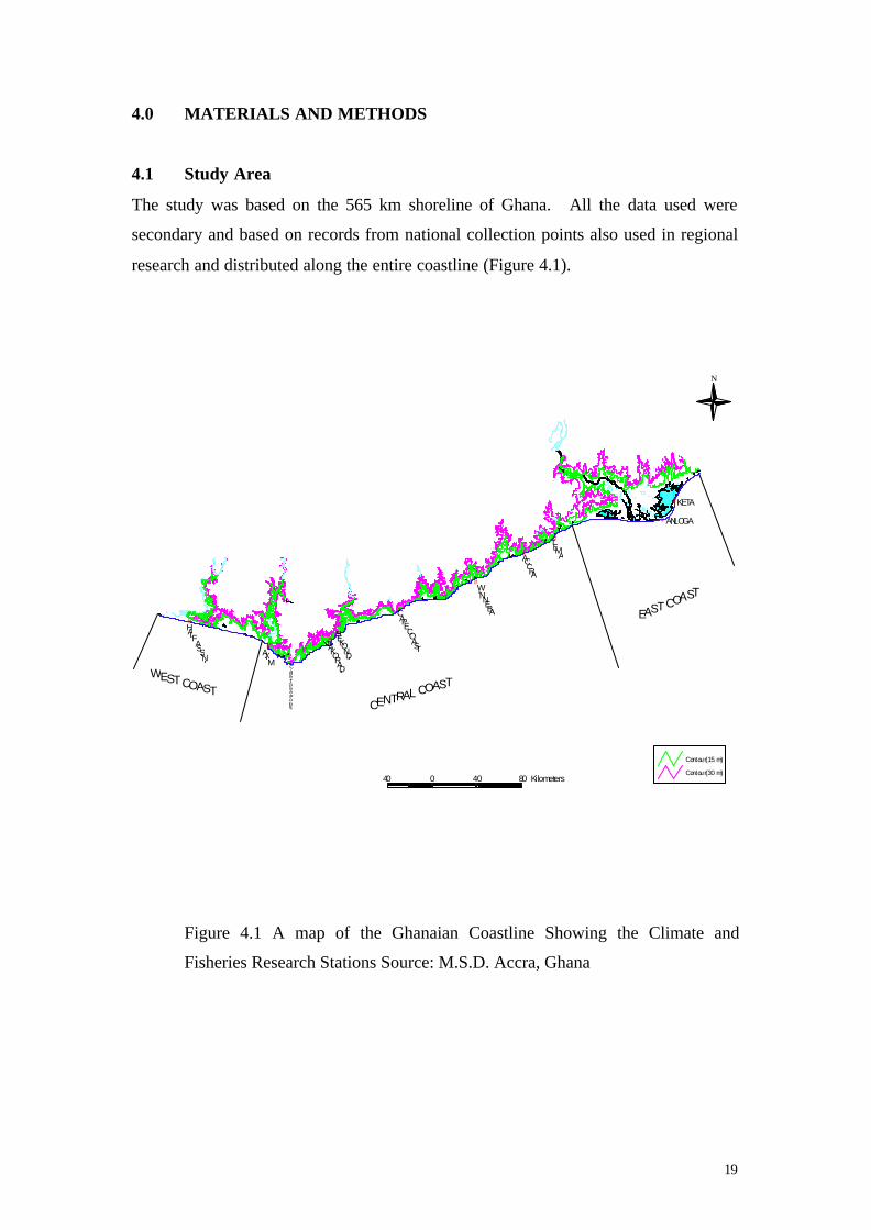
The study was based on the 565 km shoreline of Ghana. All the data used were
secondary and based on records from national collection points also used in regional
research and distributed along the entire coastline (Figure 4.1).
Figure 4.1 A map of the Ghanaian Coastline Showing the Climate and
Fisheries Research Stations Source: M.S.D. Accra, Ghana
#
#
#
#
#
##
#
#
#
HALFASSIN
IAXIM
TAKORADI
SEKONDI
CAPE
COAST
WINNEBA
ACCRA
TEMA
ANLOGA
KETA
EASTCOAST
CENTRAL COASTWESTCOAST
40 0 40 80 Kilometers
N
Contour(30 m)
Contour(15 m)
CapeThreePoints

20
4.2 Data Required and Collected Meteorological data in the form of precipitation (PPN), maximum, minimum and
mean air temperatures on land (MAT), sea surface temperatures (SST), salinity and
river run-off were required. For the fishery, all records of catch and effort data were
required.
The daily records of the maximum and minimum air temperatures from 1960-2001
were obtained from the electronic database of the Meteorological Services
Department, Accra. Daily readings of precipitation and the mean air temperature from
1961-2001 were also obtained from the same source. The values were measured at six
coastal stations along the coast as depicted in Figure 4.1. These six stations are Accra,
Ada, Tema, Takoradi, Axim and Saltpond (Nkansah, 2002). Daily records of SST
(1963-2001) and Salinity (1968-2001) were obtained from data files of the Marine
Fisheries Research Division (MFRD), Tema. These readings were taken at eight
stations: Keta, Tema, Winneba, Takoradi, Cape Three Points, Axim, Half Assini and
Elmina (Quaatey, 2002).
The annual landings (metric tonnes) and average price per kilo for the canoe and
shrimp fisheries were compiled from the MFRD’s annual summaries of Marine Fish
Production from 1961 to 2001 (MFRD, 2001). The best record of fishing effort was
culled from past reports and technical papers of the Department (Quaatey, 2002).
All the data obtained are considered authentic and are used by the organisations
responsible for both national and international studies.
4.3 Analysis Materials
Annual means for the air temperatures, salinity and sea surface temperature were
computed and put into a time series database created in MS Excel together with the
total of all readings for the precipitation, fish catch and the effort. The Multivariate
Statistical Software for Canonical Community Ordination in MS Windows
(CANOCO 4) and the Biomass Dynamic Model were used in the analysing the
meteorological and fishery data respectively.

21
4.4 Methodology
4.4.1 Biological and Economic Production of stocks
The general production trend and annual revenue obtained by species was assessed
and the most significant stocks identified. The catch, effort and SST data was filtered
and smoothened by comparison with the most recently used data analysed by
Anakwah and Santos (2002) and from the same source.
4.4.2 Meteorological data
The investigation of past climatic trends was performed by means of correlation
analyses of the MAT, SST and PPN and Salinity. The salinity value for 1995, which
was unavailable, was interpolated by finding the average of the preceding and
following years.
However, Pearson’s correlation allows only pairwise analysis of variables. For a
simultaneous analysis of all climatic variables (common time-series 1972-2001), a
multivariate analysis was called for. The data were log transformed and analysed with
the Multivariate Statistical Software for Canonical Community Ordination in MS
Windows (CANOCO 4, ter Braak & Smilauer 1998). Linear models and correlation
matrices were utilised in the ordination by means of Principal Component Analysis
(PCA). The relationships among climatic variables with and without the effect of the
annual trends (year as a covariate), and with the temperature of the previous year as
the explanatory variable were assessed. The aim was to find a parsimonious set of
environmental variables that adequately described the past climate. The selected
variables were later combined with catch rate data into a fishery-environmental
model.
4.5 Fishery Models
The stock dynamics were simulated using a biomass-dynamic model with observation
error estimation (Hilborn & Walters 1992; Haddon 2001). The exploited population
was assumed to grow according to the (logistic) Schaefer model described by the
following difference equation:
tt
ttt CKB
rBBB −−+=+ )1(1 …………………………………………..Equation 1
22
where Bt is the biomass of the stock in year t, r is the population growth rate (i.e. the
difference between birth and death rates), K (or Bmax) is the maximum population
size, and Ct the yield in year t.
The basic information required to fit the model was a time-series of yield (Ct ) and
effort (Et) for that fishery. The biomass of the stock was projected forward from the
first year in the series, given an estimate of the initial biomass (BI or B0). The
observed catch per unit effort (cpue) was assumed to be linearly related to the
abundance of the stock through a constant catchability term q:
tt
ttt qB
EC
cpueI ===∧
The caret symbol is used because an index of abundance is estimated from the model.
It is the difference between an estimated I (=qBt) and the observed I (=Ct/Et) that is
used to fit the model to reality. The observation error assumes that the model exactly
describes the population dynamics but that the observations were made with error:
εeqBEC
I tt
tt ==
∧∧
This implies that the residual error (e) is multiplicative and log-normally distributed
with a constant variance.
In the base model, the catchability variable was sometimes modified to reflect the
effect of increasing fishing effort with the relation:
tinct qqq 0= …………………………………………………………….. Equation 2
where qt is the catchability in year t and q0 is the catchability in the first year of the
series. Catchability could therefore show annual proportional increases. For a 0%
increase in catchability qinc =1, and for a 5% per annum increase qinc=1.05. The values
of qt were estimated using the closed-form procedure of Haddon (2001) because the
model is easier to fit when it has fewer directly estimated parameters. The classical
performance estimators derived from this model were the maximum sustainable yield
(MSY), the corresponding effort (EMSY) and the instantaneous fishing mortality rate at
MSY, FMSY. All these estimators should be regarded as long-term averages rather than
unique (constant) values for the population.
23
4.5.1 The Fit of the Model
The base model utilised here includes five parameters B0, r, K, q0 and qinc from
which the values of interest for fishery management are calculated. The model
parameters were obtained using lognormal residuals by two alternative methods: the
least-squares criterion
2)ln(min ∑ ∧t
t
t
I
I and the log- likelihood criterion
)1)(2)2((2
++−=∧
σπ LnLnn
LL for which n is the number of observations and
∑∧
∧ −=
t
tt
nILnILn 2
2 )(σ
Similar results are obtained with both methods. The fits were performed using Solver
in MS Excel.
4.5.2 Refinement of the Base Model (Covariates)
The time-series of catch and effort for the different species were relatively long and
this allowed the inclusion of other explanatory variables (covariates) into the base
model. The covariates that seemed more appropriate to include were the sea-surface
temperatures (T, in oC) and precipitation (P, in mm), for reasons explained before. It
was assumed in all formulations that linear changes in these environmental variables
would result in proportional changes in the output.
Two hypotheses were tested in addition to the base model. Firstly that changes in the
environmental variables would result in changes in the catchability of the fish, and
thereby in the estimated cpue:
)()( minmin PPbTTattt tt eeqBI −−
∧= …………………………………………Equation 3
where Tt and Pt are the average temperature and total precipitation in year t
respectively, Tmin and Pmin are the minimum values in the two series, and a and b are
the rate parameters for temperature and precipitation, respectively.
The second hypothesis was that these environmental variables directly influenced the
growth of the population rather than its catchability:
)()(0
minmin PPbTTat
tt eerr −−= …………………………………………….Equation 4

24
where rt is the annual growth rate of the population, which will thereby vary from
year to year depending on the observed temperature, precipitation, or both, and r0 is
the rate at the origin (i.e. at Tmin, Pmin or the two combined). In relation to the base
model, the fishery-environment model has one (e.g., a or b) or two (e.g., a and b)
extra parameters, depending on the number of environmental variables included in the
fit.
4.5.3 Selection of the Best Model
Analysis of residuals (estimated I versus observed I) after fitting the models was the
most important tool in checking for acceptable error structure and model fit. Two
criteria normally used to select robust and parsimonious models (Quinn and Deriso
1999) were also employed. The Akaike information criterion (AIC) is a means of
selecting the best model, even when the models are not hierarchical (i.e. nested):
pLLLnAIC 22 +−=
where Ln LL is the log- likelihood, and p is the number of model parameters. The AIC
was calculated for candidate models, and the most parsimonious one was that with the
lowest AIC. An alternative criterion is the Bayesian information criterion (BIC)
defined as:
)(2 nLnpLLLnBIC +−=
where n is the number of observations. The BIC forms an approximation to Bayes
factors, an important consideration when the model is used for forecasting. The AIC
tends to be a conservative criterion in that a model with more parameters results than
when using the BIC, but the BIC is more likely to result in a parsimonious model.

25
5.0 RESULTS
5.1 Trends in Climatic Parameters
The analysis showed certain features of the climatic variables that may be attributed
to naturally occurring variability or atmospheric warming. The summary of variations
is shown in Appendix 1.
5.1.1 Temperatures
Both maximum and minimum air temperatures increased by 2.5 and 2.2oC
respectively between 1960 and 2001 (Appendix 2A). Thus, MAT also increased by
about 0.9oC and a positive autocorrelation with a significant lag of one year was
observed. The highest MAT was recorded in 1998 (27.8oC) and the lowest in 1975
(26.3oC) as shown in Figure 5.1. Except for the marked decreases between 1972 and
1975, variability was generally low. An analysis of Variance indicated that the linear
regression trend was statistically significant (p-value of 0.00009) as shown in
Appendix 2B.
Figure 5.1 Trends in Mean Annual Air Temperature along the Coast of Ghana.
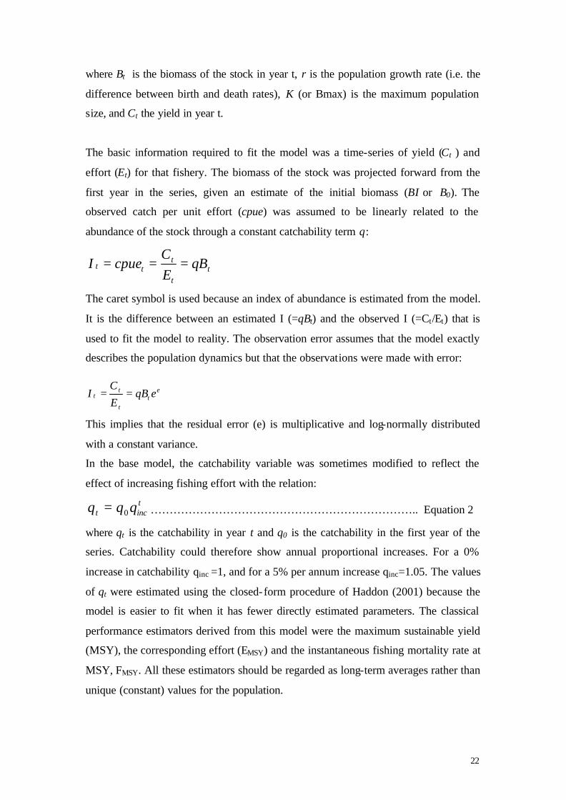
A comparison of the present SSTs with that used by Anakwah and Santos (2002)
showed minimal variation between the two data sets. (Appendix 3B). The SST (Fig.
5.2) showed a higher variability with more frequent and greater inter-annual changes
than the MAT. Cooling periods seemed to alternate with warm periods at an average
cycle of two to four years but the most significant interannual change occurred
between 1983 –84 and 1986-87. There was a slight but non-significant (p= 0.153)
increase in SST with time (Appendix 3A).
y = 0.0159x - 4.5543R2 = 0.3293
25.5
26
26.5
27
27.5
28
1960 1970 1980 1990 2000 2010Year
Tem
pera
ture
(o C
)
26
Figure 5.2 Trends in SST along the Coast of Ghana
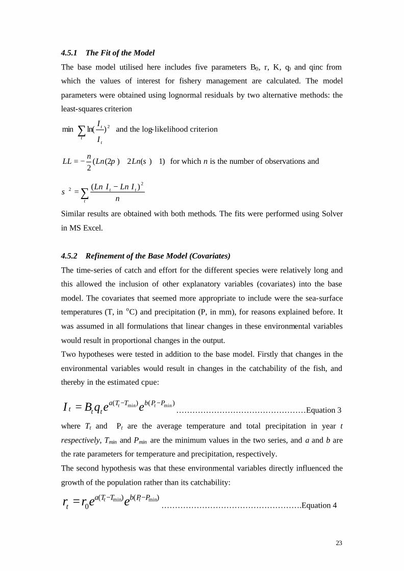
5.1.2 Salinity
This data series was the shortest and poorest of the lot due to unavailability of
historic readings. The value for 1995 had to be interpolated by finding the average of
the readings for the previous and ensuing years. For the first two years, the readings
were too low (31.10 & 32.95 ppt respectively), implying an almost impossible drastic
increase from 1968-72 (Fig. 5.3). Between 1983 and 1996, there was no clear trend. A
positive autocorrelation was, however, observed between 1970 and 1994 implying an
expected increase in salinity over the years.
Figure 5.3 Salinity Observations (1968-2001)
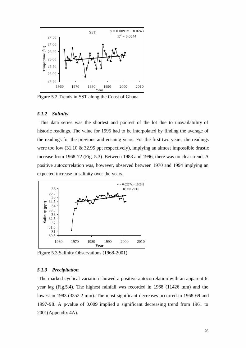
5.1.3 Precipitation
The marked cyclical variation showed a positive autocorrelation with an apparent 6-
year lag (Fig.5.4). The highest rainfall was recorded in 1968 (11426 mm) and the
lowest in 1983 (3352.2 mm). The most significant decreases occurred in 1968-69 and
1997-98. A p-value of 0.009 implied a significant decreasing trend from 1961 to
2001(Appendix 4A).
SST y = 0.0091x + 8.0243R 2 = 0.0544
24.50
25.00
25.50
26.00
26.50
27.00
27.50
1960 1970 1980 1990 2000 2010Year
Tem
pera
ture
(o C
)
y = 0.0257x - 16.248R2 = 0.2939
30.531
31.532
32.533
33.534
34.535
35.536
1960 1970 1980 1990 2000 2010Year
Salin
ity
(ppt
)
27
Figure 5.4 Precipitation Trend (1961 –2001).
The variability of the parameters described above is also observed in plots of annual
deviations from the mean (Appendices 4B-5C). The seasonal trends mentioned in
chapter 2 were reflected in the graphical summary of all the historic data (Appendices
6A – 7A).
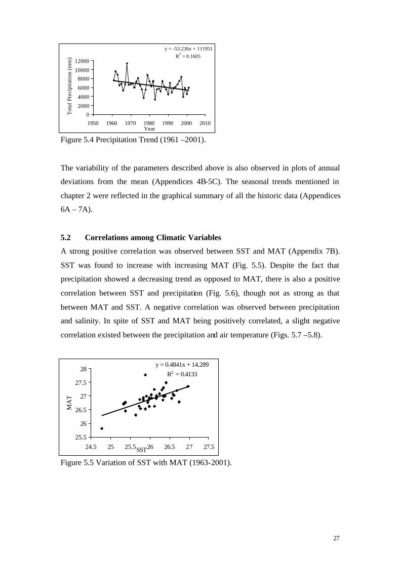
5.2 Correlations among Climatic Variables
A strong positive correla tion was observed between SST and MAT (Appendix 7B).
SST was found to increase with increasing MAT (Fig. 5.5). Despite the fact that
precipitation showed a decreasing trend as opposed to MAT, there is also a positive
correlation between SST and precipitation (Fig. 5.6), though not as strong as that
between MAT and SST. A negative correlation was observed between precipitation
and salinity. In spite of SST and MAT being positively correlated, a slight negative
correlation existed between the precipitation and air temperature (Figs. 5.7 –5.8).
Figure 5.5 Variation of SST with MAT (1963-2001).
y = -53.236x + 111951R2 = 0.1605
02000
4000
6000
800010000
12000
1950 1960 1970 1980 1990 2000 2010Year
Tot
al P
reci
pita
tion
(mm
)
y = 0.4841x + 14.289R2 = 0.4133
25.5
26
26.5
27
27.5
28
24.5 25 25.5 26 26.5 27 27.5SST
MA
T

28
Figure 5.6 Variation of Coastal Precipitation with SST
Figure 5.7 Variation of Precipitation with Mean Air Temperature
Figure 5.8 Variation of Salinity with Changes in Precipitation
These relationships were confirmed by the PCA and RDA in CANOCO 4 and are
summarised in the multivariate analysis biplots (Figures. 5.9 – 5.12).
y = -8E-05x + 35.329R2 = 0.094
3434.234.434.634.8
3535.235.435.6
0 2000 4000 6000 8000 10000Precipitation
Salin
ity
y = 1735.5x - 38828R2 = 0.2522
0
2000
4000
6000
8000
10000
12000
24.5 25 25.5 26 26.5 27 27.5SST
Prec
ipita
tion
y = -497.15x + 19857
R2 = 0.0107
0
2000
4000
6000
8000
10000
12000
25.5 26 26.5 27 27.5 28Precipitation (mm)
MA
T (o
C)

29
Fig 5.9 PCA Showing Correlation among Climatic Variables (Log-transformed
Species from 1970 to 2001). SAL = Salinity, MAT = Mean Air Temperature, PPN =
Precipitation, SST = Sea Surface Temperature
Figure 5.10 PCA Showing Correlation among Climatic Variables from 1970 -2001
(Log-transformed Series with Year as Covariate).

30
Figure 5.11 RDA Showing Correlation among Climatic Variables (Log-transformed
Data with the Previous Year’s Temperature (MAT-1) as an Explanatory Variable).
Figure 5.12. RDA Showing Correlation among Climatic Variables (Log-transformed
Data with Year as a Covariate to Filter the Annual Trends.

31
The pattern of residuals remained the same even after removal of the major time
trends (figure 5.11- 5.12). SST showed a strong positive correlation with the MAT
and PPN showed a strong negative correlation with salinity. Simultaneously, years of
high SST and MAT corresponded to years of higher salinity. These correlations were
also observed in plots of the seasonal variability (Appendices 6A-7A). The mean air
temperature of the previous year also seemed to determine the magnitude of the
parameters in the current year. The higher the MAT in the previous year, the higher
the current SST and precipitation and the lower the salinity and MAT.
5.3 Projected Climatic Scenarios
Forecasts for the next 20 years indicated that a continual decrease in the precipitation
would result if the current climatic trend were maintained (Figure 5.13). By 2021, the
precipitation could fall to an average value of 4361 cm with 6005 and 2718 cm being
the upper and lower 95% confidence limits respectively. Figure 5.13. Projected
Rainfall for the Coast of Ghana for 2002 – 2021, Based on Regression of Historical
Data (1961 – 2001).
For the forecasts of SST two scenarios could be envisaged:
(a) The observed increasing trend could not be statistically demonstrated owing to
undue variability of the historical data (type II statistical error). In the case of type
II error, avoidance, the regression line could be extrapolated (Figure 5.14). There
is considerable uncertainty about future values in year 2021 with the confidence
limits varying from 25.9 to 26.9 oC (95% lower and upper confidence limits). The
best estimate for 2021 would be 26.40 oC.
0
2000
4000
6000
8000
10000
12000
1940 1960 1980 2000 2020 2040Year
Tot
al A
nnua
l Rai
nfal
l (m
m)
Trend in PPNPPN Series
up 95%low 95%

32
Figure 5.14 Projected SST Scenario for the Coast of Ghana for years 2002 –2021
Based on Regression of Historical Data (1961-2001)
(b) If the mean trend of historical is rejected to avoid type I statistical error, the mean
of the historical data can give an indication of the expected mean temperature in
the future. (5.15).
For 2021, the expected mean SST is 26.1oC with the 95% lower and upper confidence
limits of 26.2 and 25.9oC (5.15).
Figure 5.15 Projected Mean SST Scenario for the Coast of Ghana Based on
Regression of Historical Data (1961 –2001).
24.525
25.526
26.527
27.5
1960 1980 2000 2020 2040Year
SST
(oC
)SSTSSTup 95%low 95%
24.525
25.526
26.527
27.5
1960 1980 2000 2020 2040Year
SST
(o C)
up 95%
low 95%SST

33
5.4 Production Trends of the Canoe Fishery
The most significant contributors to revenue were the round sardine, flat sardine and
anchovy (decreasing order of significance). Of the average annual revenue obtained
from the five species under study between 1980 and 2001 (C46,939,615), the Round
Sardinella, Flat Sardinella, Anchovy, Chub Mackerel and Guinea Shrimp constituted
57%, 24%, 11%, 7% and 1% respectively. The most significant stock in terms of yield
was the Anchovy followed by the Round Sardinella, Flat Sardinella, Chub mackerel
and the Guinea Shrimp (Figures 5.16 - 5.17). The prices of each species and revenues
obtained are summarised in Appendix 13.
Figure 5.16 Relative Significance of the Five Species in Terms of Revenue to the
Canoe Fleet (1980 –2001)
Figure 5.17 Relative Significance of the Five Species in Terms of Yield to the Canoe
Fleet (1980-2001)
57 %
11 %
24 %
7 % 1 %Round Sardinella
Flat SardinellaAnchovyChub Mackerel
Guinea Shrimp
41 %
10 %
43 %
5 % 1 %
Round SardinellaFlat SardinellaAnchovyChub MackerelGuinea Shrimp

34
5.5 Dynamic Production Model
The effect of fishing effort coupled with climate on the catch dynamics were best
observed for the anchovy, Round Sardinella and Flat Sardinella. The observed
parameters are presented in Tables 5.1-5.3.
The first fit performed concerned the base model. Climatic forcing was introduced in
the CPUE-based model and r-based models. In the CPUE based models, the base
model was combined with a function (equation 3) that modified catchability and
thereby expected CPUE in terms of SST, PPN or both (CPUE f (T, P)). Another
family of models utilised these covariates to change the population growth rate (rf
(T,P)) in agreement with equation 4, combined in the base model. This gave rise to
seven models fitted to each species.
Table 5.1 Production Model Estimates for the Anchovy (1974 –2001)
Parameter r K MSY qinc a b AIC BIC Base model 0.13 1,010,162 32447 1.04 0 0 45.47961 52.14064 CPUE f (T) 0.12 1036443 30502 1.05 0.028246 0 48.23129 56.22452 CPUE f (T, P)
0.12 1036581 30498 1.03 0.02983 9.66E-07 49.11555 58.44098
CPUE f (P) 0.13 1012795 32976.74 1.04 0 1.3E-05 47.26677 55.26 r f (T) 0.05 679641.7 7869.94 1.01 1.690865 0 31.74402 39.73725 r f (T, P) 0.38 206581.3 19563.63 0.96 0.954672 -5.5E-06 33.64584 42.97127 r f ( P) 0.00 2042.547 0.18 1.11 0 -0.00293 42.28003 50.27326
Table 5.2 Production Model Estimates for the Round Sardinella (1973 –2001)
Parameters r K MSY qinc a b AIC BIC Base model 0.36 620953 56174 1.17 0.00 0.00 59.50 66.34 CPUE f(T) 0.36 626315 56022 1.17 -0.04 61.28 69.48
CPUE f(T, P) 0.35 630736 55677 1.16 0.15 -9E-05 62.08 71.65 CPUE f(P) 0.35 630736 55189 1.17 0.00 -3E-05 60.73 68.93 r f(T) 1.50 3551752 1331907 0.98 -1.02 0.00 41.68 49.88 r f(T,P) 1.50 8650234 3243838 0.98 -0.86 -2.3E-05 42.81 52.38 r f( P) 0.68 712838 121477 1.01 0.00 -7.9E-05 47.86 56.06

35
Table 5.3 Production Model Estimates for the Flat Sardinella (1972 –2001)
Parameter r K MSY qinc a b AIC BIC Base model 0.336 500,000 42058 1.04 0 0 46.91 53.57 CPUE f (T) 0.336 500,000 42058 1.04 0.0073 0 48.90 56.89
CPUE f (T, P)
0.336 500,000 42058 1.04 0.028 -1.57E-05 51.28 60.60
CPUE f ( P) 0.5 600000 75000 1.00 0 2.97E -06 51.41 59.41 r f (T) 0.322 549959 44245 0.99 0.115 0 44.43 52.42 r f (T, P) 5.99E-05 405489 6.073 1.04 0.028 -1.6E-05 36.81 46.13 r f (P) 0.5 600000 75000 0.97 0 0.00203 35.43 43.42
In most cases the introduction of climatic variables improved the fit of the fishery
model and this was reflected in both the distributions of residuals and fit statistics
such as AIC and BIC (Figures 5.18-5.26). The increase in efficiency fishing effort
(technological creep) was reflected in values of qinc > 1.
The Anchovy showed the highest variability in CPUE and sensitivity to climatic
changes. Runs of the r-based model had MSY, BI, qinc, K and r, which showed much
greater variation compared to the CPUE-based model. Catch rates could increase
variably from 2.8% (for CPUE-base model) to about 169% (for r-based model) as a
result of a 1oC increase in temperature. Precipitation seemed to have a minimal
positive effect on the production of the CPUE of anchovy and a slight negative effect
on catches of the r-based model. The stock level fell gradually between 1974 to 1986
after which it shot from about 80000 to nearly 200000 mt by 1990. In 1992, it reduced
to about 120000mt. Between then and 1999, there was little variation about 150000
mt until an eventual reduction to 117391 mt in 2001 (Figures 5.18-5.20). By virtue of
the observed fluctuations the stock could not be described as an increasing or
decreasing one. It would be more appropriate to call it a variable stock that responds
to current climatic conditions.
36
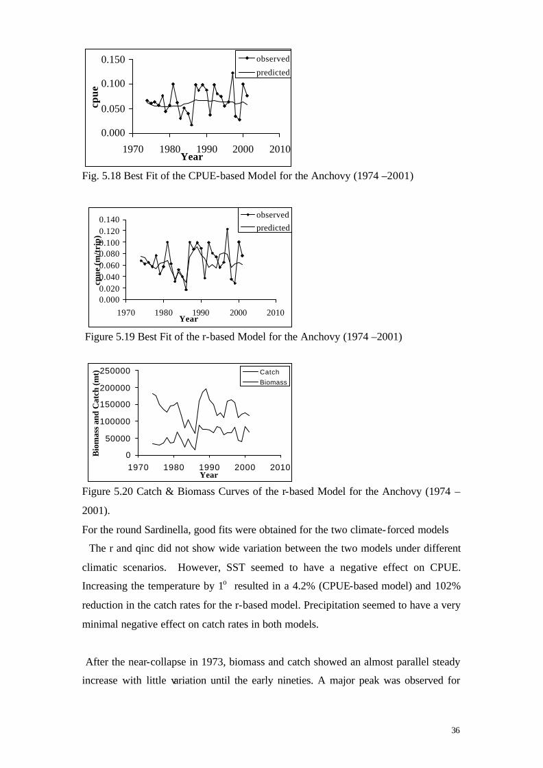
Fig. 5.18 Best Fit of the CPUE-based Model for the Anchovy (1974 –2001)
Figure 5.19 Best Fit of the r-based Model for the Anchovy (1974 –2001)
Figure 5.20 Catch & Biomass Curves of the r-based Model for the Anchovy (1974 –
2001).
For the round Sardinella, good fits were obtained for the two climate-forced models
The r and qinc did not show wide variation between the two models under different
climatic scenarios. However, SST seemed to have a negative effect on CPUE.
Increasing the temperature by 1o resulted in a 4.2% (CPUE-based model) and 102%
reduction in the catch rates for the r-based model. Precipitation seemed to have a very
minimal negative effect on catch rates in both models.
After the near-collapse in 1973, biomass and catch showed an almost parallel steady
increase with little variation until the early nineties. A major peak was observed for
0.0000.0200.0400.0600.0800.1000.1200.140
1970 1980 1990 2000 2010Year
cpue
(m/t
rip)
observedpredicted
0
50000
100000
150000
200000
250000
1970 1980 1990 2000 2010Year
Bio
mas
s an
d C
atch
(mt) Catch
Biomass
0.000
0.050
0.100
0.150
1970 1980 1990 2000 2010Year
cpue
observed
predicted

37
both in 1992 followed by a decreasing trend with the exception of a lower peak in
2000. The biomass then declined to 233664 mt in 2001 (Figs. 5.21 -5.23). These
variations were indicative of the matured fishery in which a further increase in effort
could deplete the stock.
Figure 5.21 SST-Dependent Fit for the Round Sardinella in the CPUE- based model
(1973-2001).
Figure 5.22 Best Fit for the Round Sardinella in the r-based Model (1973-2001).
Figure 5.23 Catch & Biomass curves of the r-based Model for the Round Sardinella
(1973 –2001).
0
100000
200000
300000
1970 1980 1990 2000 2010YearBio
mas
s an
d C
atch
CatchBiomass
0.000
0.050
0.100
0.150
1970 1980 1990 2000 2010Year
cpue
observed
predicted
0.000
0.050
0.100
0.150
1970 1980 1990 2000 2010Year
cpue

38
However, for the CPUE –based model, the best fit was obtained with PPN as the
covariate and suggests that precipitation had a greater effect on the distribution than
the SST (Figure 5.24).
Figure 5.24 Best Fit of the CPUE-Based Model for the Round Sardinella (1973 –
2001).
The Flat Sardinella showed the least response to SST effects and the highest response
to changes in precipitation. The catchability was best described with SST as covariate
while the r-based model had the best fit when the population growth rate depended
only on precipitation. Thus, distribution of the fish is more dependent on the
temperature while the population growth rate is more influenced by precipitation.
There seemed to be a general reduction in the CPUE. The highest was in 1976. This
was followed by a sharp reduction the next two year and a more gradual continuation
of the trend until 1985. There was a sharp increase to a peak in 1987. Thereafter the
recorded peaks have been lower as observed in 1997 and 2000. The catch trends seem
relatively constant and small when compared to the stock size. Peaks for the latter
were recorded in 1974 and 1997 (Figs 5.25-5.27).
0 .000
0 .050
0 .100
0 .150
1970 1980 1990 2000 2010Year
cpue
observed
predicted

39
Figure 5.25 Best Fit of the CPUE-based Model for the Flat Sardinella (1972 –2001)
Figure 5.26 Best Fit of the Precipitation Dependent r-based Model for the Flat
Sardinella (1972 –2001)
Figure 5.27 Catch & Biomass Curves of the r-based Model for the Flat Sardinella
(1972 –2001).
0.0000.0050.0100.0150.0200.0250.0300.0350.0400.045
1970 1980 1990 2000 2010Year
cpue
(mt/
trip
)observedpredicted
0.000
0.010
0.020
0.030
0.040
0.050
1970 1980 1990 2000 2010Year
cpue
(mt/
trip
)
observed
predicted
0
200000
400000
600000
800000
1970 1980 1990 2000 2010Year
Bio
mas
s an
d C
atch Catch
Biomass
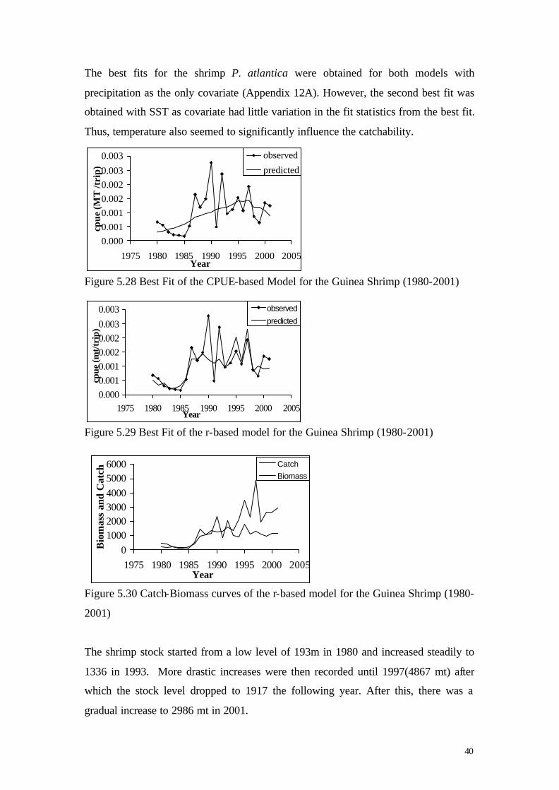
40
The best fits for the shrimp P. atlantica were obtained for both models with
precipitation as the only covariate (Appendix 12A). However, the second best fit was
obtained with SST as covariate had little variation in the fit statistics from the best fit.
Thus, temperature also seemed to significantly influence the catchability.
Figure 5.28 Best Fit of the CPUE-based Model for the Guinea Shrimp (1980-2001)
Figure 5.29 Best Fit of the r-based model for the Guinea Shrimp (1980-2001)
Figure 5.30 Catch-Biomass curves of the r-based model for the Guinea Shrimp (1980-
2001)
The shrimp stock started from a low level of 193m in 1980 and increased steadily to
1336 in 1993. More drastic increases were then recorded until 1997(4867 mt) after
which the stock level dropped to 1917 the following year. After this, there was a
gradual increase to 2986 mt in 2001.
0.0000.0010.0010.0020.0020.0030.003
1975 1980 1985 1990 1995 2000 2005Year
cpue
(mt/t
rip)
observed
predicted
0.0000.0010.0010.0020.0020.003
0.003
1975 1980 1985 1990 1995 2000 2005Year
cpue
(MT
/tri
p)
observed
predicted
0100020003000400050006000
1975 1980 1985 1990 1995 2000 2005Year
Bio
mas
s an
d C
atch
CatchBiomass
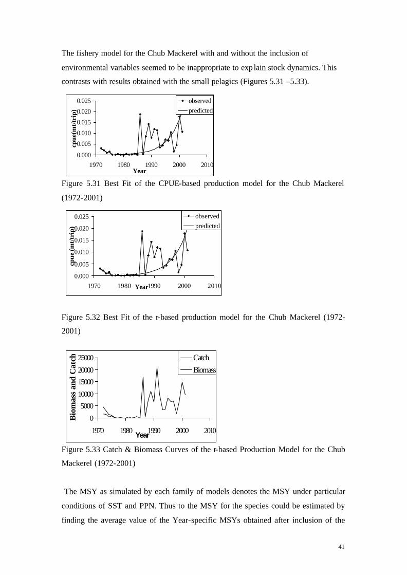
41
The fishery model for the Chub Mackerel with and without the inclusion of
environmental variables seemed to be inappropriate to exp lain stock dynamics. This
contrasts with results obtained with the small pelagics (Figures 5.31 –5.33).
Figure 5.31 Best Fit of the CPUE-based production model for the Chub Mackerel
(1972-2001)
Figure 5.32 Best Fit of the r-based production model for the Chub Mackerel (1972-
2001)
Figure 5.33 Catch & Biomass Curves of the r-based Production Model for the Chub
Mackerel (1972-2001)
The MSY as simulated by each family of models denotes the MSY under particular
conditions of SST and PPN. Thus to the MSY for the species could be estimated by
finding the average value of the Year-specific MSYs obtained after inclusion of the
0
5000
10000
15000
20000
25000
1970 1980 1990 2000 2010Year
Bio
mas
s an
d C
atch Catch
Biomass
0.000
0.005
0.010
0.015
0.020
0.025
1970 1980 1990 2000 2010Year
cpue
(mt/
trip
)
observedpredicted
0.000
0.005
0.010
0.015
0.020
0.025
1970 1980 1990 2000 2010Year
cpue
(mt/t
rip)
observedpredicted

42
SST into the fishery model. The level of fishing of the two most significant stocks can
therefore be judged from the number of times they have been overfished.
Thus, whereas the cpue-based models for the Anchovy state that the stock is
overfished, the r-based model (the best fit) says that the MSY has only been overshot
during nine out of the 28 years (Appendix 14). This occurred in the particularly in
early years of the series until the 1980's when there was a marked decline in the stock
(cool period). This implies that SST mostly causes variations in landings in spite of
the overfishing component. For the Round Sardinella, the cpue-based models indicate
overfishing while the r-based model shows that the MSY has never been reached.
That is, the SST has mostly caused the variations in the landings (Appendix 15).
From all the observations obtained, climatic factors seemed to exert a significant
influence on the production of the three most significant small pelagics and the
shrimp. Catches varied from year to year depending on the magnitude of SST and
precipitation influence. This means that the MSY for each stock is not a constant
value but varies from year to year depending on the climatic condition.

1
6.0 DISCUSSION
The MAT and precipitation are the most significant indicators of change in the
climate system. The SST and salinity seem to be direct responses of the ecosystem to
variation of the former two factors. According to the multivariate analysis, years of
higher SST should have corresponded to those of higher precipitation but this was not
reflected in the rainfall pattern and forecasts.
6.1 Climatic Trends: Merely Local Changes?
The increases in the maximum, minimum and mean air temperatures may well be
associated with the suspected trend for the sub-region or simply a result of long-term
natural variability. The 0.5oC increase in average daily coastal temperatures was 50%
lower than the value obtained for the national vulnerability assessment to climate
change from 1961 to 1990 (Republic of Ghana, 2000). This could be attributed to the
fact that the coastline falls under the coldest climatic zone.
The total decrease in precipitation (about 27.7%) was higher than the 20% observed
for the whole country between 1961 and 1990. Again, this could be explained by the
fact that the coastline is also the area with the highest precipitation. Although a
decrease in rainfall has been projected for the inland areas, an almost contradictory
increase has been predicted for the coast. This could be also be explained as follows:
1. The presence of the high forest zone near Axim implies a higher evapo-
transpiration rate during warmer temperatures, which would be accompanied by
higher rainfall (Republic of Ghana, 2000).
2. The ocean influences the coastal atmosphere by affecting its moisture content.
With atmospheric warming come greater currents and intensified upwelling. This
causes higher evaporation of water and hence increased rainfall (Brown et. al.,
1989).
However, there seems to be general conformity with predictions of overall or seasonal
decreases in tropical areas as opposed to the reverse, which would occur at higher
latitudes (IPCC, 2001).
Despite a clear warming trend for MAT and its correlation with SST, there was no
significant warming of water temperatures. This could be a reflection of the ‘Latent

2
Heat’ effect. Oceans have a buffer effect that enables them to absorb and store heat
much more effectively than the land. Thus heat uptake and loss result in a smaller
surface temperature change than would occur on land. According to Banks and Wood
(2002), SST is commonly useful in detecting changes in ocean climate because it
provides a good signal-to-noise ratio. Its distribution is also a major factor influencing
atmospheric circulation in the form of winds and precipitation (Brown et. al. 1989).
The alternating pattern in SST was in conformity with the findings of Hardman-
Mountford and McGlade (2002) for the interannual SST variations in the entire Gulf
of Guinea. Cooling occured from 1982 to 1986 and warming from 1987-1990 with
exceptional warming in 1984. By virtue of the frequency of occurrence, the 3-year
peaks were linked to El Nino events, particularly in 1984. The upwelling index
showed a similar inverse pattern with a weak upwelling in 1984 and between 1987
and 1990. An interannual variability of 3year-frequency indicative of the Atlantic El
Nino was observed to impact on the interannual upwelling intensity. The trend in SST
anomalies in Cananeia - Brazil observed by Koranteng (1998) in Tema- Ghana at a
lag of three years, and the pattern of anomaly in precipitation and river discharge in
the Ghanaian inshore area (decline between 1970 and 1983), also show that climatic
trends in the Atlantic could be related to the Pacific ENSO.
Thus, previous postulates of interaction of the global climate system with the coastal
one under study could be acceptable.
6.2 Yield-Climate Interactions
The wide interannual variations for the individual species confirm that fishing effort
alone does not account for the variations in CPUE. According to Koranteng (1991),
the erratic fluctuations in abundance of the small pelagics are due to differences in the
amounts of fish available to the fishermen, which in turn depend on coastal upwelling,
rainfall, recruitment and migratory pattern of the fish. Mensah and Quaatey (2002)
also reported that the increasing trend obtained for the small pelagics are due mainly
to the intensity of upwelling. Hence, an assessment of and projections about the
fishery cannot be made without due consideration of the climatic influences.
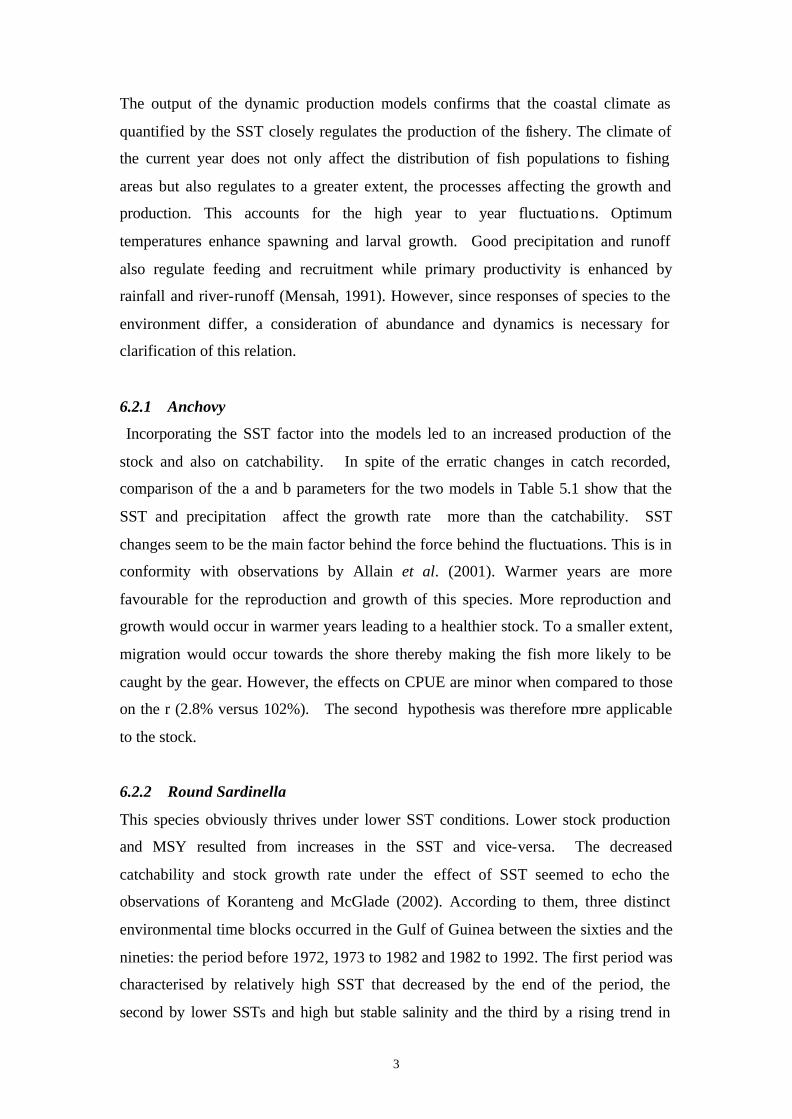
3
The output of the dynamic production models confirms that the coastal climate as
quantified by the SST closely regulates the production of the fishery. The climate of
the current year does not only affect the distribution of fish populations to fishing
areas but also regulates to a greater extent, the processes affecting the growth and
production. This accounts for the high year to year fluctuations. Optimum
temperatures enhance spawning and larval growth. Good precipitation and runoff
also regulate feeding and recruitment while primary productivity is enhanced by
rainfall and river-runoff (Mensah, 1991). However, since responses of species to the
environment differ, a consideration of abundance and dynamics is necessary for
clarification of this relation.
6.2.1 Anchovy
Incorporating the SST factor into the models led to an increased production of the
stock and also on catchability. In spite of the erratic changes in catch recorded,
comparison of the a and b parameters for the two models in Table 5.1 show that the
SST and precipitation affect the growth rate more than the catchability. SST
changes seem to be the main factor behind the force behind the fluctuations. This is in
conformity with observations by Allain et al. (2001). Warmer years are more
favourable for the reproduction and growth of this species. More reproduction and
growth would occur in warmer years leading to a healthier stock. To a smaller extent,
migration would occur towards the shore thereby making the fish more likely to be
caught by the gear. However, the effects on CPUE are minor when compared to those
on the r (2.8% versus 102%). The second hypothesis was therefore more applicable
to the stock.
6.2.2 Round Sardinella
This species obviously thrives under lower SST conditions. Lower stock production
and MSY resulted from increases in the SST and vice-versa. The decreased
catchability and stock growth rate under the effect of SST seemed to echo the
observations of Koranteng and McGlade (2002). According to them, three distinct
environmental time blocks occurred in the Gulf of Guinea between the sixties and the
nineties: the period before 1972, 1973 to 1982 and 1982 to 1992. The first period was
characterised by relatively high SST that decreased by the end of the period, the
second by lower SSTs and high but stable salinity and the third by a rising trend in

4
SSTs. These time blocks are believed to have influenced the S. aurita fishery in
Ghana and La Côte d’Ivoire as follows: a healthy phase before the high landings of
1972, a ‘collapsed’ phase from 1973 to 1982 and a phase of recovery from 1983 to
1992. These are clearly observed in the development of CPUE and stock biomass
shown in Figures 5.21-5.24. The a components for the CPUE and r-based models
(4% and 102%) also show that the population growth rate is much more variable to
climate than the distribution. The second hypothesis is also more applicable to the
round sardine than the first.
6.2.3 Flat Sardinella
The relative insensitivity of the stock to changes in SST (0.7%) as clearly reflected in
the CPUE-based model indicates that the distribution and catchability of this species
are hardly affected by changes in the ocean climate. The first hypothesis seems
inappropriate to account for the changes in the production and can be rejected. On the
other hand, the a component for the r-based model (11.5%) explains why this species
thrives during the warm season and is more tolerable to changes in SST and salinity.
The higher sensitivity of the r-based model to precipitation emphasizes the lower
sensitivity of the growth rate to SST changes.
6.2.4 Guinea Shrimp and Chub Mackerel
Precipitation was the environmental variable that strongly influenced both the
catchability and population growth rate of the guinea shrimp (Appendix 12A). Being
an estuarine shrimp that spawns in the coastal lagoons and is washed out during
adulthood into the ocean. Periods of higher precipitation are more favourable for its
distribution or migration into the coastal fishing area. Increase in precipitation lead to
higher river runoff and the washing of nutrients into coastal lagoons that harbour this
species. Salinity is also regulated by precipitation. The fit statistics obtained with the
SST as covariate also signify that the SST also affects the stock to some extent.
Studies by Haas et al., (2001) showed that 24% of the interannual variability in
offshore catch of the brown shrimp (Penaeus aztecus Ives) was explained by
environmental variables viz. water temperature, salinity, turbidity, river flow rate,
acres of suitable habitat, and precipitation. Fifty-five percent of the remaining
variation was accounted for by biological variables in the model that was used. Later,
Haas et al., (2001) confirmed that early juvenile abundance, salinity and temperature
5
are the key regulators of adult abundance. Childers et al. (1990) found that
climatological forcing has direct effects on estuarine flooding regimes and
consequently affects inshore shrimp harvests while Agbesi (2002) detected that the
influence of salinity is in itself not a significant factor but becomes essential when in
combination with other factors like temperature and precipitation. Thus observed
precipitation effects rightly describe its significance with respect to shrimp production
A stock assessment for the Chub mackerel based on the current analysis would be
unrealistic. However, Perrotta et al., 2001 indicated that this species migrates from
coastal waters at higher SST values. Cury and Roy (2002) also observed a similar
behavioural pattern in S. japonicus as that in S. aurita. Migration occurs to deeper
waters during the warm season. Thus a lower abundance would be expected in a
warming climate.
6.3 Future Production
The differences in the CPUE-based models and the r-based models indicate that the
influence of the climate is exerted more on the stock production than on the
catchability. Cury and Roy (1987) studied the pelagic stocks off Côte d’Ivoire and
suggested that the introduction of the SST into a Fox production model showed that
the influence is exerted on the fish abundance rather than on their catchability. Thus
the second hypothesis would be more acceptable than the first although the first is
also applicable.
If the current trend of decrease in precipitation should continue, the yield is not
expected to be affected significantly for the round sardine, flat sardine, anchovy and
chub mackerel, though productivity will not be maximised. For the Guinea Shrimp, a
decrease in precipitation is expected to result in a lower catch. If SST changes
continue until a significant level, an increase in catch of the anchovy is expected
while a decrease would be recorded for the chub mackerel, shrimp and most
obviously in the round sardine. The flat sardine would record slight reductions in
catch. Even if the fluctuations in SST remain insignificant, the various species
populations are expected to exhibit variability according to the extent of their
correlation with this variable. For the guinea shrimp, there seems to be an
underexploitation. However, though usually harvested by the fleet, the stock seems to

6
have been underestimated since there are also commercial shrimpers operating in the
fishing area.
It is necessary to note the positive value of qinc for all the species reflects the continuing
increase in effeciency of the effort, which was recorded for the entire canoe fleet.
Mensah and Quaatey (2002) suggested that the small pelagics in the CECAF are
overexploited but are still recording high catches as a result of the intensity of the
upwellings. This inference seems to have been based on the CPUE as reflected in the
CPUE-based model of this study. According to Cury and Roy (2002) the patterns of
SST indicate a shift in the timing and intensity of the major upwelling. The rate of
warming between August and September seems to have intensified with a more
pronounced shift in the SST drop between June and July. The minor upwelling is also
believed to have intensified in favour of the round sardine. Cury and Roy’s
assessment of the SST patterns showed that this effect was unnoticeable in the
monthly SST time series but its consequence has led to the greatest changes in the
pelagic fishery observed between 1975 and 1995. Even for the demersals, this relation
was observed and attributed to ‘an environmental forcing event’ related to climate
variability, which occurred between the sixties and the nineties. With the observations
of the current study, it is obvious that SST changes and upwelling impact more on the
population growth rate thereby compensating for the any effect of overfishing. It can
therefore be accepted that the influences of climate underplay the effect of fishing
effort and should be seriously considered if any fishery is to be managed sustainably.
If these ‘small’ changes in the ocean climate (as measured by the SST) can induce
such variability, then in the face of warming climate, the fishery would expected to
experience changes which would impact on the biology of the species as well as on
the socio-economic lives of its dependants. For the Round Sardine, Chub Mackerel
and Shrimp, revenue would be expected to decrease while that for the Anchovy would
be expected to increase. Small changes would be recorded for the flat sardine. In the
face of changing precipitation, the guinea shrimp and the flat sardine would be most
affected. The decreasing trend of precipitation implies that lower catches would be
obtained for both species. These estimates are based on the assumption that pricing of
the species and factors that determine it remain constant in the future. Further, it is
assumed that the trends observed in this simple study of historical climate (a slight

7
increase in SST and a significant decrease in the precipitation) are quantitative in
nature. Should a climate change in the next 20 years bring about changes of predictive
nature, such as reversal of ocean currents, these empirical fishery models would be
poorly suited to forecast ecosystem changes.
6.4 Limitations of the Study
1. The major limitation in this study was the inability to obtain a longer time
series for fish yield to match the climatic parameters. Most related studies
have spanned longer periods for example but data series up to 50 years could
not be obtained. A longer series of fishing effort and salinity to match that of
the MAT and precipitation would have been more useful for assessing the
historic fishery-climate relation.
2. Owing to the nature of the available data (catch rates) the fishery-environment
models had simple logistic formulations.
3. The fish yield was not representative of the entire coast since it constitutes
records from only 54 out of about 200 landing sites. Thus estimates for the
MSY and CPUE may well be underestimated.
4. It would have been useful to underline the influence of precipitation by
assessing the rate of river discharge into the sea. Data on this could not be
obtained due to time and logistic constraints.
5. An exponential relationship was assumed between production and the
climatic variables, which might not necessarily be true.
6. Complete monthly records of some of the meteorological data were not
available for some stations and the averages were only based on readings for
the other stations.
7. Good theoretical models for prediction of the climate in the sea, particularly
in the Gulf of Guinea are still unavailable. Forecasts were based on simple
empirical analysis of a short series of climate data.
8. The model parameters obtained in this are with uncertainty. The impact on
future states of the stocks and corresponding catch rates, should be the target
of simulation studies

8
7.0 CONCLUSION
7.1 Lessons
The facts discussed show that the stocks exploited by the canoe fishery are not
completely immune to changes in the climate. The SST has quite a dramatic effect on
the production of the coastal fishery and its minor interannual variations should never
be dismissed as insignificant. The influence of precipitation is also essential and
cannot be ruled out. An adverse effect on the ocean climate leading to changes in
these factors would only add to the current problem of overfishing. Since variations in
the stocks are subject to global climatic changes, management of the fishery would
require a holistic approach with due consideration of the changes in the ecosystem.
7.2 Recommendations
The first step towards the solution from the scientific point of view would be to step
up the monitoring of these and other selected environmental factors on a regular basis.
Oceans and their ecosystems, as stated earlier are relatively ‘conservative and
regulative with respect to changes. A longer time is thus needed for observable
responses to atmospheric forcing. This seems a tough challenge considering the lack
of logistics and human resource demands of the management organisations in
developing countries like Ghana. However, this and the previous studies undertaken
in the Gulf of Guinea provide a firm grounding on which to base future studies.
With the current high dependence of coastal communities on the fishery it is tasking
to effectively monitor catches completely let alone to introduce controls on the effort
and the catch. However, funding by the government and international management
organisations that recognise the importance of these shared Sardinella and Anchovy
stocks could make this more practical. Innovation through research on the ecosystem
should be strongly promoted while aquaculture activities are expanded to stabilise
seafood and employment. The data, financial and human resource requirements of the
Integrated Coastal Zones Management Program should be met to ensure the
incorporation of fisheries management with other uses of the coastal area. Close co-
operation with forestry, water and other resource managers will ensure the adequacy
of management practices in all sectors affecting the fishery. Since most people in the

9
fishing communities are ignorant of the problems accompanying overfishing and
climate change, programmes of education and capacity building should be initiated in
this regard.
Considering the uncertainties that still surround the stock-climate relation, the
management policies should be flexible enough to adapt to potential changes in the
resource and market conditions. This means that the exploitation of lesser-known
species should be encouraged to ease the pressure on the main stocks.

10
REFERENCES
Agbesi E. N., 2002. Environmental Influence on Marine Pelagic Fish: Evidence from
Bioeconomic Modelling. PhD. Department of Economics University of
Portsmouth CEMARE, UK.
Allain G., P. Petitgas and Lazure P. 2001. The Influence of Mesoscale Ocean
Processes on Anchovy (Engraulis encrasicolus) Recruitment in the Bay of
Biscay Estimated with a Three-dimensional Hydrodynamic Model. Fisheries
Oceanography Volume 10 No.2 pp. 151-163. Blackwell and Sons.
Allersma E. and M. K.W. Tilman, 1993. Coastal Conditions in West Africa- A
Review in Ocean and Coastal Management Vol., pp 199- 240.
Aman A, 1999. A Multi-Data Approach to Assess the Spatio-Temporal Variability of
The Ivorio-Ghanaian Coastal Upwelling, Ocean Circulation Science derived
from the Atlantic, Indian and Arctic Sea Level Networks ed. Mitchum, G.
2000. No. 171 pp76-80
Anakwah E and. Santos J. 2002. Department of Aquatic Biosciences, Norwegian
College of Fishery Science (NFU), University of Tromsø. Norway.
Arfi R, Bouvy M, and Ménard F. 2002. Environmental Variability in a Coastal station
near Abidjan: Oceanic and continental influences in the Gulf of Guinea Large
Marine Ecosystem. Environmental Forcing & Sustainable Development of
Marine Resources. Eds. J. M. McGlade, P. Cury, K. A. Koranteng, N. J
Hardman-Mountford. The Gulf of Guinea Large Marine Ecosystem.
Environmental Forcing & Sustainable Development of Marine Resources. Ed.
K. Shemann. Elsevier Series Amsterdam, Netherlands. 391pp
Bages, M. And A. Fonteneau, 1980. Catches of the Franco-Ivory Coast – Senegal
Tuna Fleet, and Surface Temperatures in 1997. Meeting of the Standing
Committee on Research and Statistics, ICCAT- Madrid, Spain. November.
1979.Collect-Vol-Sci-Pap-Iccat; Recl-Doc-Sci-Cicta; Colecc-Doc-Cient-
Cicaa 9(1): 180-198.
Bakun, A., 1993. Global Climate Variations and Potential Impacts on the Gulf of
Guinea Sardinella Fishery in Dynamics and Use of Sardinella Resources from
Upwelling off Ghana and Ivory Coast. Eds. Bard, F. X.; Koranteng, -K. A.-
eds. Paris France. Orstom 1995 pp 60-85.
Banks K. & R. Wood, 2002. Where to look for Anthropogenic Climate Change in the

11
Ocean, Journal of Climate Vol. 15, no. 8, pp. 879-891. American
Meteorological Society, USA.
Berger A., R. E. Dickinson, John W. Kidson (1989) Eds. Understanding Climate
Change. American Geophysical Union : International Union of Geodesy and
Geophysics (IUGG) Vol .7, Washington. 187pp
Binet,-D..1997 Climate and pelagic fisheries in the Canary and Guinea currents 1964-
1993: the role of trade winds and the Southern Oscillation in LONG-TERM-
CHANGES-IN-MARINE-ECOSYSTEMS. -LES-CHANGEMENTS-A-
LONG-TERME-DANS-LES-ECOSYSTEMES-MARINS Castel, -J.-eds.
PARIS-FRANCE GAUTHIERS-VILLARS 1997 vol. 20, no. 1 pp. 177-190.
Brown J., A. Colling, D. Park, J. Phillips, D. Rothery & J. Wright, 1989. Ocean
Circulation. Oceanography Course Series, The Open University, England.
Ed. G. Bearman. Butterworth Heinemann, United Kingdom. 238 pp.
Childers DL, JW Day and RA Muller. Relating Climatological Forcing to Coastal
Water Levels in Louisiana Estuaries and the Potential Importance of El Nino-
Southern Oscillation Events in Climate Research. Oldendorf / Luhe [CLIM.
RES.], Vol. 1, no. 1, pp. 31-42.
Condrey R. and D. Fuller, 1992. The US. Gulf shrimp Fishery. Ch. 5 in Climate
Variability, Climate Change and Fisheries, ed. M. H. Glantz,
Cambridge University Press, ISBN, UK. 450 pp.
Cury, P. And C. Roy, 1987. Upwelling et Peches des Espèces Pélagique Cotieres de la
Cote d’Ivoire: Une approche globale. Oceanol. -Acta. 10 (3): 347-357
Cury P. and C. Roy, 2002. Environmental Forcing and Fisheries Resources in Côte
d’Ivoire and Ghana: Did Something Happen? pp. 241-274 In McGlade J. M,
Cury P, Koranteng K .A, Hardman-Mountford N.J, 2002 The Gulf of Guinea
Large Marine Ecosystem. Environmental Forcing & Sustainable Development
of Marine Resources. Ed. K. Shemann. Elsevier Series Amsterdam.
Demarcq H and Aman A .2002 A Multi-Data Approach for assessing the Spatio-
Temporal variability of the Ivorian-Ghanaian Coastal Upwelling:
Understanding Pelagic Fish Stock Dynamics in The Gulf of Guinea Large
Marine Ecosystem. Environmental Forcing & Sustainable Development of
Marine Resources. Eds. J. M. McGlade, P. Cury, K. A. Koranteng, N. J.
Hardman-Mountford. The Gulf of Guinea Large Marine Ecosystem.

12
Environmental Forcing & Sustainable Development of Marine Resources. Ed.
K. Shemann. Elsevier Series Amsterdam, Netherlands. 391pp
Dykhuizen P and Zei M, 1970.Clupeid Fisheries in the Eastern Atlantic. Information
Report No.3, Fisheries Research Unit, Tema, Ghana
F.A.O. 1986. Guia Campo Para as Especies Comercais Marinhas de Aguas
Salobras de Angola Fichas de Identificacao de Especies Para Actidades de
Pesca. Organizacao das Nacoes Unidas Para a Agrucultura e a Alimentacao
Rome.
FAO, 1997. Review of the State of the World Fishery Resources: FAO Fisheries
Circular No. 920 FIRM/C920, Marine Resources Services, Fishery Resources
Division, FAO, Rome.
Froese R. and D. Pauly. 2002. FishBase. World wide Web Electronic Publication.
(www.fishbase.org)
Glantz, M: H., 1992. Climate Variability, Climate Change and Fisheries, Cambridge
University Press, ISBN, UK. 450 pp.
Haas, HL, R. F Shaw. K A Rose, MC Benfield, WR Keithly 2001. Regression
Analysis of the Relationships among Life-stage Abundances of Brown
Shrimp (Penaeus aztecus) and Environmental Variables in Southern
Louisiana, USA in Proceedings of the Gulf and Caribbean Fisheries Institute
[Proc. Gulf Caribb. Fish. Inst.]. No. 52, pp. 231-241.
Haas HL, E C. Lamon III, KA Rose, RF Shaw, 2001. Environmental and Biological
Factors Associated with the Stage-specific Abundance of Brown Shrimp
(Penaeus aztecus) in Louisiana: Applying a New Combination of Statistical
Techniques to long-term monitoring data. Canadian Journal of Fisheries and
Aquatic Sciences [Can. J. Fish. Aquat. Sci./J. Can. Sci. Halieut. Aquat.]. Vol.
58, no. 11, pp. 2258-227
Haddon, N., 2001. Modelling and Quantitative Methods in Fisheries. Chapman and
Hall/CRC, USA
Hardman-Mountford, N. J. and J.M. McGlade 2002. Variability of Physical
Environmental Processes in the Gulf of Guinea and Implications for Fisheries
Recruitment. An Investigation Using Remotely Sensed SST. In The Gulf of
Guinea Large Marine Ecosystem. Eds. J. M: McGlade, P. Cury, K: A.
Koranteng & N. J. Hardman-Mountford. The Gulf of Guinea Large Marine

13
Ecosystem. Environmental Forcing & Sustainable Development of Marine
Resources. Ed. K. Shemann. Elsevier Series Amsterdam, Netherlands. 391pp
HillBorn and Waters, 1992. Quantitative Fisheries Stock Assessment: Choice,
Dynamics and Uncertainty. Chapman & Hall, London.
Horton R W., R F Shaw, J C Cope and C Benfield, 1997. Atmospheric Cold Fronts
and Coastal Ocean-estuarine Physical Forcing as a Brown Shrimp (Penaeus
aztecus) Recruitment Enhancement Mechanism. Midyear Meeting of the
Southern Division of the American Fisheries Society. San Antonio, Texas.
(www.sdafs.org/meetings/97sdafs/pollute/horton1.htm)
Houghton, J.T, 1997 An Introduction to simple climate models used in the IPCC
Second Assessment Report, IPCC Technical paper; Vol. II
IPCC, 2001. Climate Change: Impacts Adaptation and Vulnerability. A Report of
Working Group II. Technical Summary pp. 35 – 36, Summary for Policy
Makers, pp. 11 – 12. (www.ipcc.org).
Isaka, D., S. O. Minta, V. Obeng and J Sackey, 2002 A Report on Ghana’s Fisheries.
Norwegian College of Fishery Science, University of Tromsø, Norway.
Kattenberg, -A. J.; Giorgi, -F.; Grassl, -H.; Meehl, -G.A.; Mitchell,-J.F.B.; Stouffer,-
R.J., Tokioka, -T.; Weaver, -A. J.; Wigley, -T.M.L. Climate models—
Projections of Future Climate in Climate Change 1995- The Science of
Climate Change. Houghton, J. T.; Meira – Filho, L. G.; Callander, B. A.;
Harris, N.; Kattenberg, A.; Maskell, Eds. Cambridge University Press, New
York, USA
Kawasaki, T., 1992. Effects of Global Climate Change on Marine Ecosystems and
Fisheries in Climate Change: Science, Impacts and Policy, Proceedings of the
Second World Climate Conference, Ed. J. Jager and H. L. Ferguson,
Cambridge University Press, U.K.
Kerr, R. A., 1984. Computer Models Gain on El Nino. Science Wash., Vol. 225, No.
4657, pp. 37-38
King M., 1995. Fisheries Biology, Assessment and Management. Fishing News
Books, Oxford. 341pp.
Koranteng, K: A., 1991. Some Aspects of the Sardinella Fishery in Ghana. in
Pêcheries Ouest Africaines Variabilité, Instabilité et Changement. Pp. 269 –
277 Editeurs Scientifique Philippe Cury et Claude Roy ORSTOM Ed. Institut

14
Français De Recherche Scientifique Pour Le Development Et Cooperation,
Paris.
Koranteng, K.A.1999. Biodiversity Status and Threats on Demersal Fish
Communities in continental Shelf Waters of the Gulf of Guinea in
International-Workshop-on-status-of-the-freshwater; coastal; marine- living-
resources-with-particular-emphasis-on-threats-and-options- in-coastal-areas, -
15-18-november-1999-in-Montpellier,-France Vidy,-G.-(ed.); Albaret,-J.J.-
(ed.); Baran,-E.-(ed.) Montpellier-France IRD 1999 pp. p. A.3.15-16.
Koranteng K.A and McGlade J .M, 2002. Physico-Chemical Changes in Continental
Shelf Waters of the Gulf of Guinea and Possible Impacts on Resource
Variability in the Gulf of Guinea Large Marine Ecosystem. Environmental
Forcing & Sustainable Development of Marine Resources. Eds. J. M.
McGlade, P. Cury, K. A. Koranteng, N. J. Hardmann-Mountford. Elsevier
Series, Amsterdam, Netherlands. 391pp.
Laevastu T. and M. L. Hayes, 1988. Fisheries Oceanography and Ecology, 3rd Ed.
Fishing News Books Ltd. England. 199 pp.
Marine Fisheries Research Division (MFRD), 2001. Summary of Total Marine Fish
Production for Ghana. Fisheries Directorate of the Ministry of Food and
Agriculture, Tema, Ghana
McGlade J. M, Cury P, Koranteng K .A, Hardman-Mountford N.J, 2002 The Gulf of
Guinea Large Marine Ecosys tem. Environmental Forcing & Sustainable
Development of Marine Resources. Eds. J. M. McGlade, P. Cury, K. A.
Koranteng, N. J. Hardmann-Mountford. Elsevier Series
Amsterdam. 391p.
Mendelssohn, R. 1988 Relating Fisheries to the Environment in the Gulf of Guinea:
Information, Causality and Long-Term Memory. in Pêcheries Ouest
Africaines Variabilité, Instabilité et Changement. Pp. 269 –277 Editeurs
Scientifique Philippe Cury et Claude Roy ORSTOM Ed. Institut Français De
Recherche Scientifique Pour Le Deve loppement Et Cooperation, Paris
Mensah, M. A. and Koranteng, K. A., 1988. A Review of the Oceanography And
Fisheries Resources in the Coastal Waters of Ghana, 1981 –1986. Marine
Fisheries Research Report No. 8, Fishery Research Unit, 35pp.
Mensah M. A. & S.N.K Quaatey, 2002. An Overview of Fishery Resources and
Fishery Research in the Gulf of Guinea. in The Gulf of Guinea Large Marine
15
Ecosystem. Environmental Forcing & Sustainable Development of Marine
Resources. Eds. J. M. McGlade, P. Cury, K. A. Koranteng, N. J. Hardman-
Mountford. The Gulf of Guinea Large Marine Ecosystem. Environmental
Forcing & Sustainable Development of Marine Resources. Ed. K. Shemann.
Elsevier Series Amsterdam, Netherlands. 391pp
Mensah, M. A.1991. The Influence of Climatic Changes in the Coastal Oceanography
of Ghana in Pêcheries Ouest Africaines Variabilité, Instabilité et Changement.
Pp. 67 –79. Editeurs Scientifique Philippe Cury et Claude Roy ORSTOM Ed.
Institut Français De Recherche Scientifique Pour Le Developpement Et
Cooperation, Paris
Nkansah A, 2002. Meteorological Services Department, Accra, Ghana.
Perrotta RG, MG Vinas, Hernandez DR, Trigali L. 2001 Temperature conditions in
the Argentine chub mackerel (Scomber japonicus) fishing ground:
implications for fishery management Fisheries Oceanography [Fish.
Oceanography.]. Vol. 10, no. 3, pp. 275-283
Quaatey, S. N. K., 1996. Report on the Synthesis of Recent Evaluations Undertaken
On the Major Fish Stock in Ghanaian Waters, Marine Fisheries Research
Division, Fisheries Directorate of the Ministry of Food and Agriculture, Tema,
Ghana.
Quaatey S. N. K., 2002. Marine Fisheries Research Division, Fisheries Directorate of
the Ministry of food and Agriculture, Tema, Ghana.
Quinn T. S. II and Deriso R. B.1999. Quantitative Fish Dynamics. Oxford Univerity
Press. New York
Republic of Ghana, 2000. Ghana’s Initial National Communication under the United
Nations Framework Convention on Climate Change, Environmental
Protection Agency, Accra- Ghana.
Rothschild, B. 1996. How Bountiful are Ocean Fisheries? CONSEQUENCES: 2. No1.
(www. gcrio.ciesin.org/CONSEQUENCES/winter96/oceanfish.html)
Roy,-C..1993. The Cote-d'Ivoire and Ghana Coastal Upwellings Dynamics and
Changes Dynamics-and-use-of-Sardinella-resources-from-upwelling-off-
Ghana-and-Ivory-coast.-DYNAMIQUE-ET-USAGE-DES-RESSOURCES-
EN Bard,-F.X.-eds.; Koranteng -K.A.-eds. Paris-France ORSTOM 1995 pp.
346-361.
Roy, C. 1996. An Upwelling Induced Retention Area off Senegal: A Mechanism to

16
Link Upwelling and Retention Processes in South African Journal of Marine
Science 1998. Vol. 19 pp. 89-98.
Schnur R, 2002 Climatic Science: The forecast. Nature Vol.415, No.6871. pp 483-
484.ccc Mac Millan publishers
Sharp G., 1992. Climate Change, the Indian Ocean Tuna Fishery, and Empiricism.
Ch. 16 in Climate Variability, Climate Change and Fisheries, ed. M. H.
Glantz, Cambridge University Press, ISBN, UK. 450 pp.
Sloane, Christine S and Tesche T.W, c1991, Atmospheric Chemistry: Models and
Predictions for Climate and Air Quality, Lewis Publishers, 169pp
Spencer W., 2001. The Discovery of Global Warming: General Circulation Models
of the Atmosphere Based on Edwards, P., 2000. A Brief History of
Atmospheric General Circulation Modelling in General Circulation Model
Development, Ed. David A. Randall, pp67-90. San Diego, CA: Academic
Press
ter Braak CJF and Petr Smilauer, 1998. CANOCO Reference Manual and User’s
Guide to CANOCO for Windows. Software for Canonical Community
Ordination (Version 4) Centre for Biometry, Wageningen, and Nederlands.
pp15-301
Verstraete, -J. -M.; Picaut, -J. 1983. Variation of Sea Level, Sea Surface Temperature
and Dynamic Height along the Northern Coast of the Gulf of Guinea.
OCEANOGR.-TROP. 1983. Vol. 18, no. 2, pp. 139-162

17
APPENDIX 1
Summary of Annual Variation in Climatic Variables Source MSD Database, MFRD,
Ghana * Data Unavailable
YEAR SST(o C MAT(oC) SALINITY (ppt) PRECIPITATION
(mm) MINIMUM
TEMPERATURE MAXIMUM
TEMPERATURE
1960 * * * * 23.2 29.9 1961 * 26.6 * 7602.7 23.2 30.0 1962 * 26.6 * 9651 23.2 30.1 1963 26.6 27.0 * 8857.7 23.5 30.5 1964 25.4 26.5 * 6501.2 23.0 29.9 1965 26.1 26.6 * 6864.8 23.3 30.1 1966 26.0 26.9 * 5324.7 23.6 30.0 1967 25.9 26.5 * 6711.4 23.2 29.9 1968 26.7 26.8 31.10 11426.5 23.6 30.1 1969 26.0 27.0 32.95 6594.2 23.9 30.3 1970 26.2 26.9 33.67 6696.9 23.6 30.5 1971 25.8 26.5 33.69 6928.5 23.1 30.0 1972 26.0 26.8 34.56 6014.9 23.4 30.1 1973 26.3 27.3 34.82 7303.4 23.9 30.7 1974 26.0 26.6 34.51 8155.7 23.2 29.9 1975 25.6 26.3 34.73 6411.1 22.9 29.7 1976 24.8 25.8 34.59 5586.7 23.0 29.2 1977 25.4 26.8 35.05 3667.4 23.7 30.0 1978 25.7 26.6 34.53 5534.5 23.5 29.7 1979 26.4 27.0 34.22 8766.6 23.9 30.1 1980 25.9 26.8 34.42 7370.3 23.7 29.9 1981 26.0 26.9 34.27 6270.6 23.8 30.2 1982 25.7 26.9 34.59 7426.4 24.0 30.8 1983 25.3 26.7 35.09 3352.2 24.4 30.8 1984 26.4 27.0 34.98 5569.5 24.2 31.0 1985 25.8 26.9 35.21 5778.8 24.2 30.9 1986 25.4 26.7 35.16 5115.7 23.7 30.1 1987 27.0 27.3 35.17 7422.1 24.1 30.2 1988 26.6 26.9 35.22 6235.1 23.1 30.1 1989 26.3 26.9 34.87 5602 23.2 30.3 1990 25.9 27.0 35.46 4492.6 23.3 30.1 1991 26.2 27.0 35.17 7077.3 23.5 29.8 1992 25.8 26.9 35.18 4877.9 23.6 30.3 1993 26.6 27.1 35.06 5947.8 23.8 30.5 1994 26.4 27.0 35.12 6137.8 23.7 30.3 1995 26.7 27.2 * 6715.6 23.9 30.7 1996 26.2 27.1 35.38 7460.4 24.0 30.3 1997 26.2 27.0 34.81 8405.12 23.9 30.3 1998 25.9 27.8 34.84 3893.5 24.6 31.1 1999 26.3 27.2 35.14 5901.7 23.9 30.5 2000 26.1 27.2 34.45 4519.6 24.0 30.4 2001 26.4 27.5 34.49 5953.7 25.4 32.5

18
APPENDIX 2
Appendix 2A Trends in Maximum & Minimum Air Temperature
Appendix 2B Autocorrelation Analysis: Mean Air Temperature
y = 0.0233x + 23.163R2 = 0.3429
y = 0.0191x + 29.87R2 = 0.2075
20.0
22.0
24.0
26.0
28.0
30.0
32.0
34.0
1960
1965
1970
1975
1980
1985
1990
1995
2000
Year
Tem
pera
ture
(o C)
SUMMARYOUTPUT
RegressionStatistics
MultipleR
0.573844
R Square 0.329297AdjustedR Square
0.3121
StandardError
0.274785
Observations
41
ANOVAdf SS MS F Significance F
Regression
1 1.445796 1.445796 19.14794956 8.76378E-05
Residual 39 2.944756 0.075507Total 40 4.390552
Coefficients
StandardError
t Stat P-value Lower 95% Upper 95% Lower 95.0% Upper95.0%
Intercept -4.55428 7.18503 -0.63386 0.529874569 -19.0873623 9.978801023 -19.0873623 9.978801XVariable1
0.015871 0.003627 4.375837 8.76378E-05 0.008534649 0.023206857 0.008534649 0.023207

19
APPENDIX 3
Appendix 3A Autocorrelation Analysis: Sea Surface Temperature
Appendix 3B Comparison of SST values used by Anakwah and Santos, 2002 &
Minta, 2003, 1975-1999.
SUMMARYOUTPUT
RegressionStatistics
MultipleR
0.23332
R Square 0.054438AdjustedR Square
0.028882
StandardError
0.437952
Observations
39
ANOVAdf SS MS F Significance F
Regression
1 0.408572 0.408572 2.130174334 0.152863077
Residual 37 7.096679 0.191802Total 38 7.505252
Coefficients
StandardError
t Stat P-value Lower 95% Upper 95% Lower 95.0% Upper95.0%
Intercept 8.024258 12.3502 0.649727 0.519882167 -16.99959529 33.04811107 -16.99959529
33.04811
XVariable1
0.009094 0.006231 1.459512 0.152863077 -0.00353102 0.021719686 -0.00353102 0.02172
y = 1.0019xR2 = 0.9367
24.5
25.0
25.5
26.0
26.5
27.0
27.5
24.5 25 25.5 26 26.5 27 27.5
Minta, 2003
Ana
kwah
, 200
2
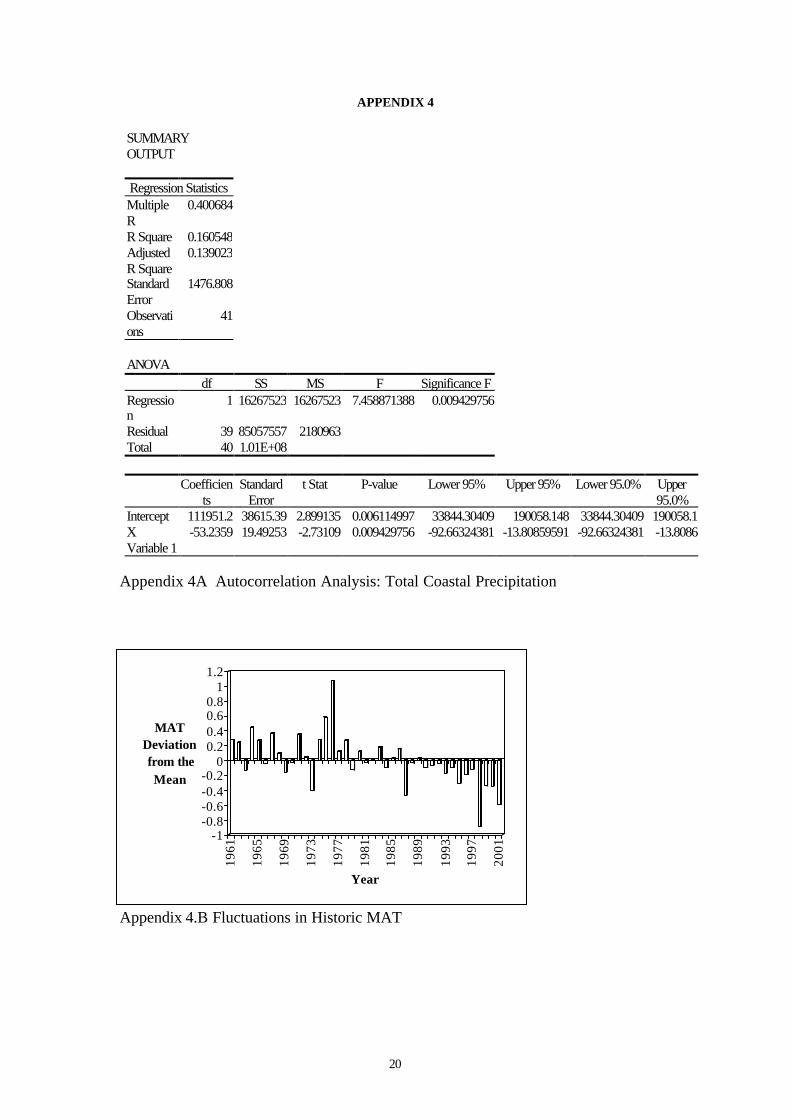
20
APPENDIX 4
Appendix 4A Autocorrelation Analysis: Total Coastal Precipitation
Appendix 4.B Fluctuations in Historic MAT
SUMMARYOUTPUT
Regression StatisticsMultipleR
0.400684
R Square 0.160548AdjustedR Square
0.139023
StandardError
1476.808
Observations
41
ANOVAdf SS MS F Significance F
Regression
1 16267523 16267523 7.458871388 0.009429756
Residual 39 85057557 2180963Total 40 1.01E+08
Coefficients
StandardError
t Stat P-value Lower 95% Upper 95% Lower 95.0% Upper95.0%
Intercept 111951.2 38615.39 2.899135 0.006114997 33844.30409 190058.148 33844.30409 190058.1XVariable 1
-53.2359 19.49253 -2.73109 0.009429756 -92.66324381 -13.80859591 -92.66324381 -13.8086
-1-0.8-0.6-0.4-0.2
00.20.40.60.8
11.2
MAT Deviation from the Mean
1961
1965
1969
1973
1977
1981
1985
1989
1993
1997
2001
Year
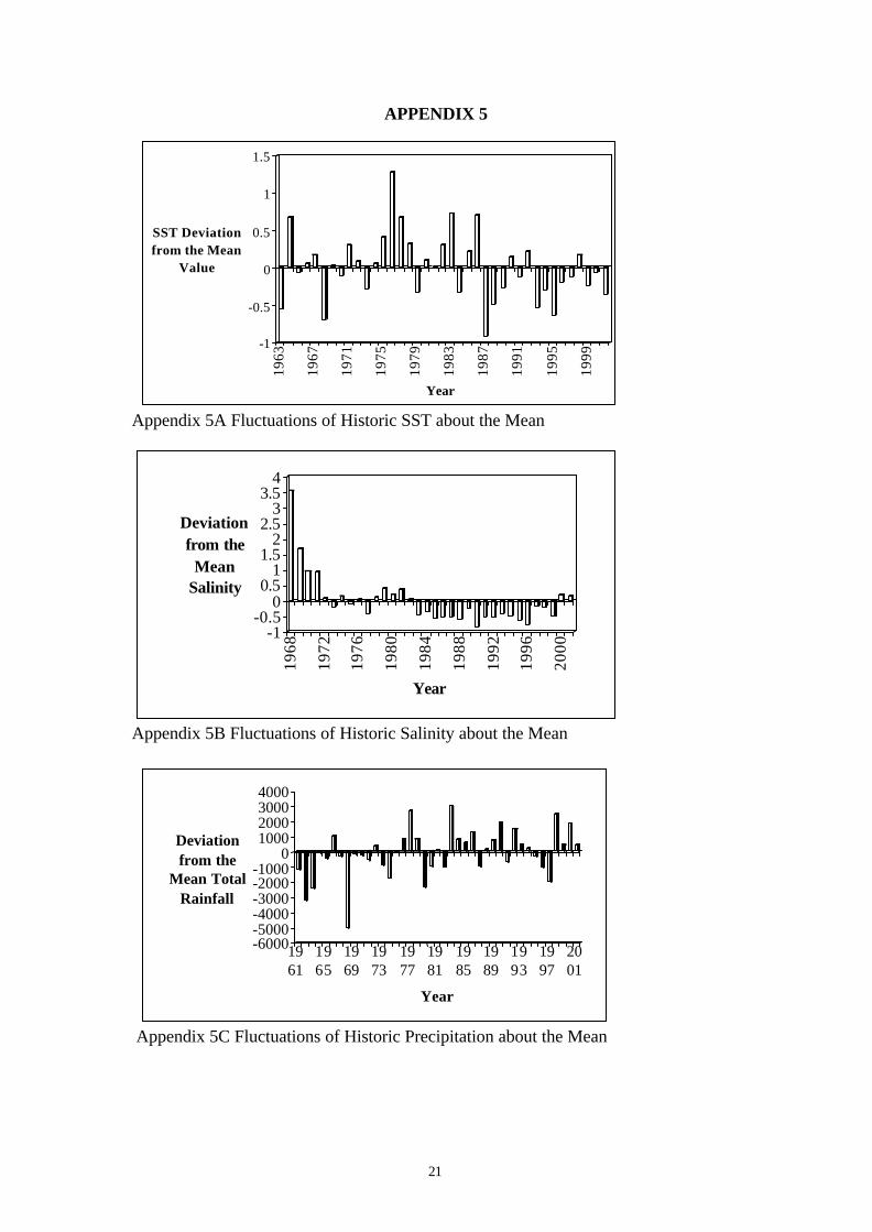
21
APPENDIX 5
Appendix 5A Fluctuations of Historic SST about the Mean
Appendix 5B Fluctuations of Historic Salinity about the Mean
Appendix 5C Fluctuations of Historic Precipitation about the Mean
-1
-0.5
0
0.5
1
1.5
SST Deviation from the Mean
Value19
63
1967
1971
1975
1979
1983
1987
1991
1995
1999
Year
-1-0.5
00.5
11.5
22.5
33.5
4
Deviation from the
Mean Salinity
1968
1972
1976
1980
1984
1988
1992
1996
2000
Year
-6000-5000-4000-3000-2000-1000
01000200030004000
Deviationfrom the
Mean TotalRainfall
1961
1965
1969
1973
1977
1981
1985
1989
1993
1997
2001
Year

22
APPENDIX 6
Appendix 6A Seasonal Variation of MAT (based on 1961-2001)
Appendix 6B Seasonal Variation of Precipitation (Based on 1961-2001)
Appendix 6C Seasonal Variation of Salinity (Based on 1968-2001)
23.023.524.024.525.025.526.026.527.027.528.028.5
Temperature (oC)
Jan
Feb
Mar
Apr
May Jun
Jul
Aug
Sep
t
Oct
Nov dec
Month
0.0
50.0
100.0
150.0
200.0
250.0
300.0
Total Precipitation
(mm)
Jan
Feb
Mar
Apr
May
Jun
Jul
Aug
Sep
t
Oct
Nov de
c
Month
33.600
33.800
34.000
34.200
34.400
34.600
34.800
35.000
35.200
Jan
Feb
Mar
Apr
May Jun
Jul
Aug
Sept
Oct
Nov de
c

23
Appendix 7
Appendix 7A Seasonal Variation of Maximum and Minimum Temperature (Based
on 1960 – 2001)
Appendix 7B Results of Correlation Analysis for Climatic Variables Measured along
the Coast of Ghana
0.0
5.0
10.0
15.0
20.0
25.0
30.0
35.0
Jan Feb
Mar Apr May Jun Ju
lAug Sep
tOct No
vdec
Month
Tem
per
atu
re (o
C)
MaximmumMinimum
Pearson CorrelationsSST MAT SAL PPN
SST 1.000 0.643 -0.167 0.502MAT 1.000 0.134 -0.103SAL 1.000 -0.593PPN 1.000
PearsonProbabilities
SST MAT SAL PPNSST 0.000 0.000 0.317 0.001MAT 0.000 0.424 0.536SAL 0.000 0.000PPN 0.000

24
APPENDIX 8 Appendix 8A. Regression Statistics for Precipitation Trend along the Coast of Ghana Multiple R 0.400684 R Square 0.160548 Adjusted R Square
0.139023
Standard Error 1476.808 Observations 41
ANOVA
df SS MS F Significance F Regression 1 16267523 16267523 7.458871 0.00943 Residual 39 85057557 2180963 Total 40 1.01E+08
Coefficien
ts Standard
Error t Stat P-value Lower
95% Upper 95%
Lower 95.0%
Upper 95.0%
Intercept 111951.2 38615.39 2.899135 0.006115 33844.3 190058.1
33844.3
190058.1
X Variable 1 -53.2359 19.49253 -2.73109 0.00943 -92.6632
-13.80
86
-92.66
32
-13.8086
Appendix 8B Regression Statistics for SST Trend along the Coast of Ghana Multiple R 0.2333198
47
R Square 0.054438151
Adjusted R Square
0.028882425
Standard Error 0.437952222
Observations 39
ANOVA df SS MS F Significance F
Regression 1 0.408572014
0.408572
2.130174
0.152863
Residual 37 7.0966795 0.191802
Total 38 7.505251514
Coefficients
Standard Error
t Stat P-value Lower 95%
Upper 95%
Lower 95.0%
Upper 95.0%
Intercept 8.024257888
12.35019775
0.649727
0.519882
-16.9996
33.04811
-16.9996
33.04811
Year 0.009094333
0.006231079
1.459512
0.152863
-0.00353
0.02172 -0.00353
0.02172

25
APPENDIX 9
Appendix 9 Annual Production of the Major Marine Stocks in Ghana. Source: MRFD
* Data Unavailable
Year Species Catch (mt) Effort
(trips)
Round
Sardinella
Flat
Sardinella
Anchovy Chub
Mackerel
Guinea
Shrimp
1972 71267.4 3001 * 1682.4 * 538751
1973 3074.5 7537.3 * 1543.3 * 698196
1974 1408.1 16110.9 33440.8 484.7 * 496180
1975 1931.1 18328.5 32172.1 832.7 * 520989
1976 12008.7 17472 28656.6 71.6 * 442201
1977 9581.6 14696 35042.9 93.3 * 613729
1978 40257.3 11069.5 51424.1 304.2 * 672414
1979 9247.4 14249.1 36675.9 51.8 * 827836
1980 19426.1 11310.1 37908.1 43.4 451.9 662540
1981 10066.5 12445.3 67535.5 327.4 385.8 676161
1982 20110.4 12378.3 46435 87.9 230.3 745190
1983 36299 7667.6 24392.3 194.9 163.4 787211
1984 34816.3 10077.1 47230.9 540.3 172.5 908052
1985 54072.5 22233.9 27590.3 45.2 106.8 695981
1986 45488.9 16633.5 15208.5 16865.7 482.6 897500
1987 45670.7 25479.2 87984.4 397.3 1455.4 3546324
1988 75851.5 10450.4 75902.3 7423.5 1039.8 867841
1989 61158.5 14097.7 76347.9 11035.8 1152.9 773203
1990 43166.5 14549 74668.1 6671.9 2326.4 839811
1991 50447 8206.7 65490 21028.5 865.2 1757136
1992 119514.7 14240.3 85384.4 9819.2 2042.4 860681
1993 90600.4 16797.1 81349.7 3455.5 977.9 1009118
1994 67565.6 12309.5 60519.3 3554.7 907.4 813104
1995 65597.5 13091.6 65496.7 8323.1 1798.3 1168906
1996 77866.2 13038.5 66552 6852.3 1104.5 1028128
1997 46383.9 14069.7 82723.6 7086.1 1303.1 674750
1998 54595.6 14770.3 44643.7 1972 1109.8 1269328
1999 48498.2 12850.1 39840 6572.9 922.3 1418903
2000 98864.7 14934.9 83500.8 14835.4 1130.6 834937
2001 64103.6 15853.4 68174.6 9574.3 1121.6 892534

26
Appendix 10
Appendix 10A Fluctuation in Landings of Round Sardinella in Relation to SST
Deviations from the Mean
Appendix 10B Fluctuation in Landings of Flat Sardinella in Relation to SST
Deviations from the Mean
Appendix 10C Fluctuation in Landings of the Anchovy in Relation to SST Deviations
from the Mean.
0
20
40
60
80
100120
140
160
1972
1975
1978
1981
1984
1987
1990
1993
1996
1999
Year
CPU
E (k
g/tr
ip)
-1.5
-1
-0.5
0
0.5
1
1.5
SST
Dev
iatio
n fr
om M
ean
rssstdev
0
10
20
30
40
50
1972
1975
1978
1981
1984
1987
1990
1993
1996
1999
Year
CP
UE
(kg/
trip
)
-1.5
-1
-0.5
0
0.51
1.5SS
T D
evia
tion
from
th
e M
ean(
o C)
fssstdev
0
20
40
60
80
100
120
140
1972
1975
1978
1981
1984
1987
1990
1993
1996
1999
Year
CPU
E (k
g/tr
ip)
-1.5
-1
-0.5
0
0.5
1
1.5
SST
Dev
iatio
n(o C
)
ancsstdev

27
APPENDIX 11
Appendix 11A Fluctuation in Landings of the Chub Mackerel in Relation to SST
Deviations from the Mean
Appendix 11B Fluctuation in Landings of the Guinea Shrimp in Relation to SST
Deviations from the Mean
Appendix 11C Model Estimates for the Chub Mackerel (1972 – 2001)
Parameter r K MSY qinc a b AIC BIC
Basic 0.01 517112.8 1292.8 1.2235- - 105.0598 110.5151CPUE f(T) 0.3 50000 3750 1.2235 0- 107.0598 113.6061
CPUE f(T, P)
0.3 4000 3000 1.2235 0.1 0 109.6067 117.2439
CPUE f(P) 0.4 5000 500 1.2235- 0 107.0598 113.6061
r f(T) 0 33537.6 0 1.2235 0.4- 107.0598 113.6061r f (T, P) 0 517112.8 0 1.2235 0.025.2546E -
05 109.06 116.70
r f (P) 0.7 22599 3954.8 1.2235- 0.000128 107.0598 113.6061
0
5
10
15
20
1972
1975
1978
1981
1984
1987
1990
1993
1996
1999
Year
CP
UE
(kg/
trip
)
-1.5-1
-0.50
0.5
1
1.5
SST
Dev
iati
on fr
om th
e M
ean
cmsstdev
0
0.5
1
1.5
2
2.5
3
1972
1975
1978
1981
1984
1987
1990
1993
1996
1999
Year
CPU
E (k
g/tr
ip)
-1.5
-1
-0.5
0
0.5
1
1.5SS
T D
evia
tion
from
the
Mea
ngssstdev
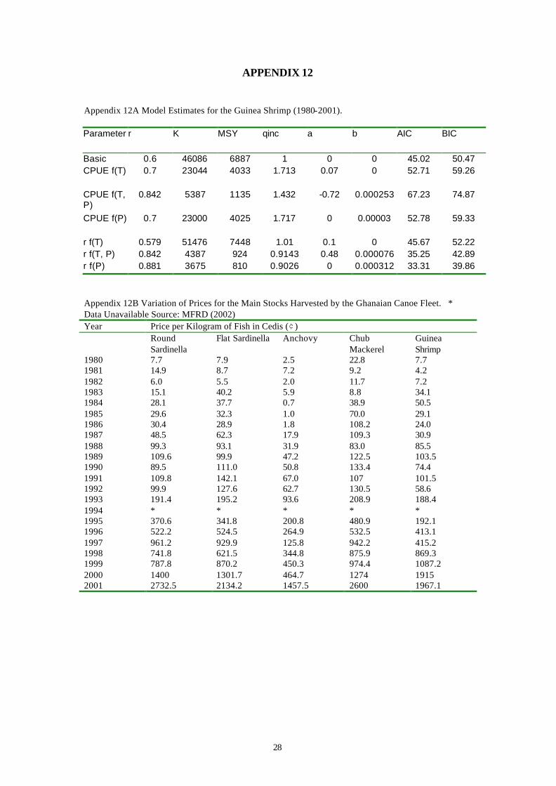
28
APPENDIX 12 Appendix 12A Model Estimates for the Guinea Shrimp (1980-2001). Parameter r K MSY qinc a b AIC BIC
Basic 0.6 46086 6887 1 0 0 45.02 50.47 CPUE f(T) 0.7 23044 4033 1.713 0.07 0 52.71 59.26
CPUE f(T, P)
0.842 5387 1135 1.432 -0.72 0.000253 67.23 74.87
CPUE f(P) 0.7 23000 4025 1.717 0 0.00003 52.78 59.33
r f(T) 0.579 51476 7448 1.01 0.1 0 45.67 52.22 r f(T, P) 0.842 4387 924 0.9143 0.48 0.000076 35.25 42.89 r f(P) 0.881 3675 810 0.9026 0 0.000312 33.31 39.86
Appendix 12B Variation of Prices for the Main Stocks Harvested by the Ghanaian Canoe Fleet. * Data Unavailable Source: MFRD (2002) Year Price per Kilogram of Fish in Cedis (¢) Round
Sardinella Flat Sardinella Anchovy Chub
Mackerel Guinea Shrimp
1980 7.7 7.9 2.5 22.8 7.7 1981 14.9 8.7 7.2 9.2 4.2 1982 6.0 5.5 2.0 11.7 7.2 1983 15.1 40.2 5.9 8.8 34.1 1984 28.1 37.7 0.7 38.9 50.5 1985 29.6 32.3 1.0 70.0 29.1 1986 30.4 28.9 1.8 108.2 24.0 1987 48.5 62.3 17.9 109.3 30.9 1988 99.3 93.1 31.9 83.0 85.5 1989 109.6 99.9 47.2 122.5 103.5 1990 89.5 111.0 50.8 133.4 74.4 1991 109.8 142.1 67.0 107 101.5 1992 99.9 127.6 62.7 130.5 58.6 1993 191.4 195.2 93.6 208.9 188.4 1994 * * * * * 1995 370.6 341.8 200.8 480.9 192.1 1996 522.2 524.5 264.9 532.5 413.1 1997 961.2 929.9 125.8 942.2 415.2 1998 741.8 621.5 344.8 875.9 869.3 1999 787.8 870.2 450.3 974.4 1087.2 2000 1400 1301.7 464.7 1274 1915 2001 2732.5 2134.2 1457.5 2600 1967.1
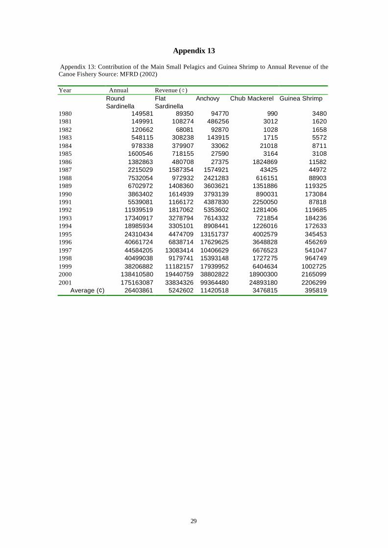
29
Appendix 13 Appendix 13: Contribution of the Main Small Pelagics and Guinea Shrimp to Annual Revenue of the Canoe Fishery Source: MFRD (2002) Year Annual Revenue (¢) Round
Sardinella Flat Sardinella
Anchovy Chub Mackerel Guinea Shrimp
1980 149581 89350 94770 990 3480 1981 149991 108274 486256 3012 1620 1982 120662 68081 92870 1028 1658 1983 548115 308238 143915 1715 5572 1984 978338 379907 33062 21018 8711 1985 1600546 718155 27590 3164 3108 1986 1382863 480708 27375 1824869 11582 1987 2215029 1587354 1574921 43425 44972 1988 7532054 972932 2421283 616151 88903 1989 6702972 1408360 3603621 1351886 119325 1990 3863402 1614939 3793139 890031 173084 1991 5539081 1166172 4387830 2250050 87818 1992 11939519 1817062 5353602 1281406 119685 1993 17340917 3278794 7614332 721854 184236 1994 18985934 3305101 8908441 1226016 172633 1995 24310434 4474709 13151737 4002579 345453 1996 40661724 6838714 17629625 3648828 456269 1997 44584205 13083414 10406629 6676523 541047 1998 40499038 9179741 15393148 1727275 964749 1999 38206882 11182157 17939952 6404634 1002725 2000 138410580 19440759 38802822 18900300 2165099 2001 175163087 33834326 99364480 24893180 2206299
Average (¢) 26403861 5242602 11420518 3476815 395819

30
APPENDIX 14 Calculation of the MSY for the Anchovy Using Annual Values Estimated by Incorporation of the SST Factor Year SST(oC) r_T MSY_t Catch (mt) No. Of Years with
Catch>MSY 1974 25.9833333 0.357331 60714.31 33440.8 1975 25.6416667 0.200527 34071.7 32172.09 1976 24.775 0.046318 7869.939 28656.6 1 1977 25.375 0.127747 21705.58 35042.9 1 1978 25.725 0.23087 39227.28 51424.1 1 1979 26.375 0.692923 117734.8 36675.9 1980 25.9416667 0.333023 56584.02 37908.1 1981 26.0416667 0.394373 67008.08 67535.5 1 1982 25.7416667 0.237469 40348.47 46435 1 1983 25.325 0.117391 19945.95 24392.3 1 1984 26.375 0.692923 117734.8 47230.9 1985 25.8333333 0.277282 47113.03 27590.3 1986 25.35 0.12246 20807.18 15208.5 1987 26.9666667 1.884368 320173.7 87984.4 1988 26.55 0.931522 158275.4 75902.3 1989 26.325 0.636749 108190.3 76347.9 1990 25.9083333 0.314772 53483.03 74668.1 1 1991 26.1666667 0.48719 82778.75 65490 1992 25.8333333 0.277282 47113.03 85384.4 1 1993 26.5833333 0.985533 167452.3 81349.7 1994 26.35 0.664242 112861.7 60519.3 1995 26.6833333 1.16709 198300.8 65496.7 1996 26.2416667 0.553062 93971.01 66552 1997 26.1666667 0.48719 82778.75 82723.6 1998 25.8833333 0.301743 51269.34 44643.7 1999 26.3 0.610394 103712.2 39840 2000 26.1083333 0.441431 75003.71 83500.8 1 2001 26.4083333 0.733099 124561.2 68174.6
Average 0.510939 86813.95 55081.8 Total No. Of times Catch>MSY=9

31
APPENDIX 15
Calculation of the MSY for the Round Sardinella Using Annual Values Estimated by
Incorporation of the SST Factor
Year SST r_T MSY_t Catch(MT) 1973 26.34167 0.30552 271282.8 3074.5 1974 25.98333 0.439642 390374.9 1408.1 1975 25.64167 0.622024 552319 1931.1 1976 24.775 1.5 1331907 12008.7 1977 25.375 0.815517 724128.7 9581.6 1978 25.725 0.571544 507495.2 40257.3 1979 26.375 0.29535 262252.1 9247.4 1980 25.94167 0.458647 407249.8 19426.1 1981 26.04167 0.414351 367918.2 10066.5 1982 25.74167 0.56195 498976.7 20110.4 1983 25.325 0.858001 761852 36299 1984 26.375 0.29535 262252.1 34816.3 1985 25.83333 0.511993 454617.8 54072.5 1986 25.35 0.83649 742750.9 45488.9 1987 26.96667 0.16194 143792.7 45670.7 1988 26.55 0.247255 219546.8 75851.5 1989 26.325 0.310736 275914.1 61158.5 1990 25.90833 0.47444 421273.5 43166.5 1991 26.16667 0.364948 324051.6 50447 1992 25.83333 0.511993 454617.8 119514.7 1993 26.58333 0.239024 212238.3 90600.4 1994 26.35 0.302945 268996.4 67565.6 1995 26.68333 0.215939 191740.6 65597.5 1996 26.24167 0.338181 300283.8 77866.19 1997 26.16667 0.364948 324051.6 46383.9 1998 25.88333 0.486641 432107.3 54595.63 1999 26.3 0.318727 283009.6 48498.2 2000 26.10833 0.387224 343830.8 98864.7 2001 26.40833 0.285518 253522.1 64103.6
AVERAGES 0.465408 413253.6 45092.17