An Assessment of the Flux Profile Method for Determining Air–SeaMomentum and Enthalpy Fluxes from Dropsonde Data in

Tropical Cyclones

DAVID H. RICHTER AND RACHEL BOHAC

Department of Civil and Environmental Engineering and Earth Sciences, University ofNotre Dame, Notre Dame, Indiana

DANIEL P. STERN

University Corporation for Atmospheric Research, Monterey, California

(Manuscript received 2 November 2015, in final form 4 March 2016)

ABSTRACT

An analysis of the reliability of using dropsonde profile data to compute surface flux coefficients of mo-mentum and heat is performed. Monin–Obukhov (MO) similarity theory forms the basis for the flux profilemethod, where mean profiles of momentum, temperature, and moisture are used to estimate surface fluxes,from which bulk flux coefficients can then be determined given surface conditions. The robustness of thismethod is studied in terms of its sensitivity to internal, method-based parameters, as well as the uncertaintydue to variability in the measurements and errors in the estimates of surface conditions, particularly seasurface temperature. In addition, ‘‘virtual sondes’’ tracked through a high-resolution large-eddy simulation ofan idealized tropical cyclone are used to evaluate the flux profile method’s ability to recover known surfaceflux coefficients given known, prescribed surface conditions; this provides a test of whether or not MO as-sumptions are violated and under which regions they hold. Overall, it is determined that the flux profilemethod is only accurate within 50% and 200% for the drag coefficient CD and enthalpy flux coefficient CK,respectively, and thus is limited in its ability to quantitatively refine model estimates beyond typically usedvalues. Factors such as proximity to the storm center can cause significant errors in both CD and CK.

1. Introduction

The specification of bulk flux coefficients in high windsover the ocean has been the subject of much debate inthe past two decades. These coefficients, which ultimatelydetermine the surface fluxes of momentum, heat, mois-ture, and other scalars, are a highly idealized represen-tation of surface transport and are typically cast asfunctions only of near-surface (typically 10m) windspeed. At low wind speeds (less than, say, 20m s21),the general behavior of these transfer coefficients is wellpredicted by bulk parameterizations such as the COAREalgorithm (Fairall et al. 2003; Edson et al. 2013); in highwinds, particularly within tropical cyclones, however,large degrees of observational uncertainty preclude any

consensus on their specific behavior. For instance, be-ginning with the efforts of Powell et al. (2003), it is nowgenerally believed that the drag coefficient CD eithersaturates or peaks in high winds, but many details of thissaturation process, including the exact ‘‘roll off’’ windspeed or the ultimate physical cause of this plateau, remainunknown. Furthermore, it is becoming increasingly clearthat CD is a function of other factors, particularly waveproperties, which can cause modifications of near-surfaceatmospheric turbulence, leading to a systematic spread inthe CD versus wind speed formulation (Holthuijsen et al.2012; Takagaki et al. 2012; Reichl et al. 2014; Sullivanand McWilliams 2010).While many studies attempt to measure the drag co-

efficient at high winds (Powell et al. 2003; Jarosz et al.2007; Troitskaya et al. 2012; Vickers et al. 2013; Frenchet al. 2007; Donelan et al. 2004; Potter et al. 2015), farfewer attempt to measure or constrain the thermody-namic flux coefficients. The Humidity Exchange Over

Corresponding author address: David Richter, University ofNotre Dame, 156 Fitzpatrick Hall, Notre Dame, IN 46556.E-mail: david.richter.26@nd.edu

JULY 2016 R I CHTER ET AL . 2665

DOI: 10.1175/JAS-D-15-0331.1

! 2016 American Meteorological Society

the Sea (HEXOS) program (DeCosmo et al. 1996)measured sensible and latent heat fluxes using eddycovariance from a fixed platform in the North Sea andfound no statistically significant trend, albeit with ex-pected observational data scatter, of either the sensibleheat flux coefficient CH or the water vapor exchangecoefficient CE with wind speeds up to roughly 20ms21.From these measurements they hypothesize that theinfluence of waves and/or spray is either nonexistent orcompensated in some way to yield unchanged fluxcoefficients.The high-wind component of the Coupled Boundary

Layer Air–Sea Transfer (CBLAST) campaign produceddirect, eddy covariance sensible and latent heat fluxmeasurements made from aircraft flown through theboundary layers of Hurricanes Fabian and Isabel in 2003and found an extended range of insensitivity of CH andCE to wind speed out to nearly 30m s21 (Zhang et al.2008; Drennan et al. 2007). For these measurements, seasurface temperatures (SSTs) were estimated by adownward-looking infrared radiometer (Black et al.2007) so that surface temperature and moisture condi-tions could be used to compute the flux coefficients. Bysumming the sensible and latent heat fluxes, the totalmoist enthalpy flux coefficient CK is also found to re-main statistically constant up to 30ms21 (Zhang et al.2008). Furthermore, from other components of theCBLAST data (i.e., not just eddy covariance measure-ments, but including radar, flight-level, and microwaveradiometer data as well), Bell et al. (2012) constructedazimuthally averaged energy and angular momentumbudgets to estimate the surface fluxes of momentum andenthalpy in regions where direct measurements are un-available and concluded that CK, within a large degreeof uncertainty, remains in the same range as previousestimates, even beyond wind speeds of 70m s21.In the laboratory, attempts to measure air–sea energy

transfer have been performed for many years (Mangarellaet al. 1973), but only recently have high-wind conditionsbeen successfully achieved. Haus et al. (2010) and Jeonget al. (2012) usedwater-side energy budgets to solve for theair–water moist enthalpy flux and found once again thatthe values ofCK are relatively unchanged up to 10-m windspeeds of roughly 40ms21. While the measurement un-certainties of this dataset aremuch better constrained thanthe observationally based estimates of CK, questions re-main regarding practical laboratory limitations on factorssuch as wave age, wave height, spray, and fetch.The importance of the flux coefficients CD and CK,

and more generally of the relative balance betweenenergy dissipation through drag and energy inputthrough sensible and latent heat at the air–sea interface,has long been recognized as a key factor for accurately

predicting tropical cyclone development and intensity(Rosenthal 1971). The theoretical/numerical work ofEmanuel (1986) and Emanuel (1995) predicts that thestorm intensity will vary as the square root of the ratiobetween CK and CD, based on axisymmetric thermo-dynamic budgets of a steady-state system. Other studieshave shown the direct, substantial influences of varyingsurface flux coefficients in numerical predictions oftropical cyclone development, structure, and strength(Montgomery et al. 2010; Bryan 2013, 2012; Green andZhang 2013; Bao et al. 2011). Generally speaking, in-creases in CK lead to overall increases in storm strength,while increases to CD may nominally decrease stormstrength (as defined by the maximum 10-m wind speed),albeit through more complicated alterations to thepressure-gradient wind balance and near-surface inflow.Other studies actually exploit the sensitivity of stormstructure to surface flux coefficients to estimate the‘‘best’’ values of CD or CK using parameter estimationprocedures (Sraj et al. 2013; Green and Zhang 2014;Rios-Berrios et al. 2014).Meanwhile, it is well recognized that these transfer

coefficients are meant to represent myriad small-scaleprocesses in some sort of bulk sense. Therefore manyattempts have been made to predict high-wind fluxes ofmomentum, heat, and moisture based on parameterizedconsiderations of processes such as waves (Kudryavtsevand Makin 2007; Troitskaya et al. 2012; Reichl et al.2014) or spray (Mueller and Veron 2014; Makin 2005;Fairall et al. 1994; Andreas 2004, 2010; Veron 2015).Unfortunately, however, these often-intricate modelsare difficult to verify because of the practical difficultiesassociated with making small-scale, in situ measure-ments of quantities such as spray generation functions orhigh-wavenumber surface wave spectra. Moreover, incertain cases, appealingly sound theoretical argumentsseem at odds with uncertain measurements, whichhighlights the need for continuous improvement of both.For instance, surface enthalpy flux models that accountfor spray, including those of Andreas (2011), MuellerandVeron (2014), and Bao et al. (2011), indicate thatCK

may undergo a systematic increase with wind speedsexceeding 30ms21, which is seemingly at odds with theobservations mentioned above. The observations, how-ever, are highly uncertain at high winds and cannotconclusively rule out the predicted model behavior.It is this continued limited understanding of air–sea

thermodynamic fluxes at high winds that motivates thecurrent work. In a previous study, Richter and Stern(2014) show that mean profiles of temperature andmoisture obtained from dropsondes launched withintropical cyclones can be used to construct mean enthalpyprofiles that are fitted to estimate surface enthalpy fluxes

2666 JOURNAL OF THE ATMOSPHER IC SC IENCES VOLUME 73

[using Monin–Obukhov (MO) similarity theory—hereinreferred to as the flux profile method]. The work ofRichter and Stern (2014) specifically focuses on the evi-dence of spray-mediated enthalpy fluxes containedwithinthese profiles. Rather than focusing on the behavior ofthe flux coefficient CK, power-law scaling exponents ofthe dimensional enthalpy fluxHK versus wind speed wereused to distinguish between laboratory cases, where so-called interfacial fluxes were dominant over spray-mediatedenthalpy fluxes and field observations.The current study aims to quantify the general utility

and accuracy of the flux profile method in the context oftropical cyclone winds. The flux profile method is thebasis for the study of Powell et al. (2003), which pro-vided the first observational evidence that CD saturatesat high winds. The work of Holthuijsen et al. (2012) isalso based on the flux profile method, where the quad-rant dependence ofCDwas used to infer wave influenceson surface momentum fluxes. While each of thesestudies used profiles obtained from dropsondes, otherstudies, such as the recent work by Zhao et al. (2015),use multilevel tower data for the same purpose.Many factors exist, however, that may render in-

appropriate the use of MO theory (or, equivalently, theexistence of a logarithmic surface layer or ‘‘log layer’’) inhurricane boundary layers, including, for example, radialpressure balances near the core (Smith and Montgomery2014). The current work computes dynamic and ther-modynamic fluxes and flux coefficients based on meanvertical profiles obtained from dropsondes and discussesthe sources of uncertainty and sensitivity in this pro-cess. In addition, high-resolution large-eddy simulations,where the turbulent boundary layer is not parameterized,are used to test the ability of emulated dropsonde profilesto recover known surface temperature and flux condi-tions, thereby assessing the general ability of this methodnear the core of a simulated tropical cyclone vortex. Ingeneral, it appears that the estimates of CD are accuratewithin roughly 50%, while estimates of CK are moresubject to uncertainty and are only accurate withinroughly 200%.

2. Dropsonde data

a. Method

1) THEORY

To estimate surface fluxes from tropical cyclones, datafrom GPS dropsondes were obtained from the publiclyavailable datasets provided by theNational Oceanic andAtmospheric Administration’s (NOAA) HurricaneResearch Division (HRD). In total, 2425 dropsondeprofiles from 37 different tropical cyclones (ranging in

intensity from tropical depression to category-5 hurri-cane) were used to construct mean profiles of pressure,temperature, humidity, and wind speed. Pressure, tem-perature, and humidity are measured at a frequency of2Hz, as were winds prior to 2010. Starting in 2010, aredesigned sonde was introduced, and winds are nowmeasured at 4Hz; of the 2425 total sondes, 616 of themwere launched in 2010 or later and thus used the rede-signed sonde. The sondes are advected horizontally andvertically by the winds, while falling at a density-dependent rate, which is approximately 10–12m s21 inthe lower troposphere. Based on this fall speed, data aresampled every 5–6m vertically (;3m for wind speed forthe newer sondes). For this dataset, all sondes weredropped by either Air Force C130 or NOAAP3 aircraft,which typically fly at heights of 1.5–4 km. Therefore, thesondes typically take about 3–6min to fall to the surface.All sondes in this dataset were quality controlled byHRD, using either HRD’s Editsonde software or theNational Center for Atmospheric Research’s Atmo-spheric Sounding Processing Environment (ASPEN)software. The stated instrumental accuracy of the GPSdropsonde is 0.5mb (1mb = 1hPa), 0.28C, 2%, and0.5m s21 for pressure, temperature, relative humidity,and wind speed, respectively (Hock and Franklin 1999).The underlying basis of MO theory (see, e.g., Monin

and Yaglom 1971) is that mean gradients of velocity orother quantities (referred to here as an arbitrary scalarf) are based solely on the surface flux of that quantityand the height z above the surface (assumed to be muchlarger than a typical roughness length: z ! z0). Thus, inregions of the flow without the influence of small-scalesurface details, large-scale forcings, or elevated sourcesor sinks, dimensional analysis predicts that the meanvelocity and scalar profiles observe a logarithmicbehavior:

hui5u*k

ln

!z

z0

"and (1)

hfi2f05

f*k

ln

!z

zf

", (2)

where it is assumed that the surface conditions areneutrally stable, the surface currents (i.e., the watervelocity u0 at the surface) are negligible,1 and that thesame scaling parameter k (the von Kármán constant;

1 If a surface current u0 was somehow known and not negligible,Eq. (1) could be modified by subtracting u0 from the left-hand side.Obtaining estimates for surface currents under sonde profiles is,however, nearly impossible, and we assume that the wind speed iseverywhere much higher than u0.

JULY 2016 R I CHTER ET AL . 2667

taken to be k 5 0.4 throughout) is valid for all meanprofiles. Note that, by taking k 5 0.4 for both the ve-locity and scalar relationships, we have implicitlyassumed a turbulent Prandtl number equal to 1; that is,we assume that the turbulent diffusivity of momentumand passive scalars is identical. In general, the value maybe slightly less than unity (Monin andYaglom 1971), butfor the present purposes a value of 1 is chosen for sim-plicity. The averages denoted by h"i indicate horizontalor ensemble averages, z0 is the roughness length, whichis defined as the height at which the velocity profilebecomes equal to the (negligible) surface current, and zfis analogously the height where f attains its surfacevalue of f0.In Eq. (1), u* refers to the friction velocity, which is

defined based on the total surface stress tw:

ru2*5 t

w, (3)

where r is the air density. Likewise, in Eq. (2), f* is ascale for f determined dimensionally from the surfacescalar flux Hf:

2ru*f*5Hf, (4)

where Hf is the upward-directed surface flux of f. It isassumed that the momentum flux tw and scalar flux Hf,and thus u* and f*, are constant with height given theabove conditions. Typically, the constant surface layerfluxes are understood as the turbulent fluxes rhu0w0i andrhw0f0i in the absence of other mechanisms of verticalmomentum or scalar transfer (form stress due to waves,elevated spray sources, etc.), where the primes indicateperturbations from the mean.Finally, the bulk parameterizations of interest relate

the surface fluxes tw and Hf to reference conditions,which are often taken as the 10-m mean quantities U10

and f10:

tw5 ru2

*5 rCDU2

10 and (5)

Hf52ru*f*5 rC

fU10(f10 2f0) , (6)

where CD is the familiar drag coefficient and Cf is thebulk flux coefficient for the scalar f.Thus, as long as the aforementioned assumptions

hold—namely, negligible surface shape influences (i.e.,can be captured solely through a roughness parameter-ization), no large-scale influences, no elevated sources/sinks, and neutral stability—one can, in theory, obtainthe quantities u* and f* by determining the slope of huiand hfi plotted versus the logarithm of z (see Fig. 2).From u* and f*, the surface fluxes tw and Hf can bereadily obtained from the first equality of Eqs. (5) and

(6), which, given the surface quantity f0, can also beused to obtain CD and Cf via the second equality.In the present study, the flux coefficients for mo-

mentum CD and enthalpy CK are of particular interestand will be based on mean profiles of wind speed, po-tential temperature, specific humidity, and moist en-thalpy. Moist enthalpy is defined as the total specificenthalpy of moist air:

k5 [(12 q)cp,a 1qc

l]u1L

yq , (7)

where cp,a is the specific heat of dry air at constantpressure, cl is the specific heat of liquid water, u is thepotential temperature, Ly is the latent heat of vapor-ization, and q is the specific humidity. Note that thepotential temperature u is used in place of true tem-perature T to eliminate effects of adiabatic expansionwith decreasing pressure. In this regard, the referencepressure for converting temperature to potential tem-perature is the pressure recorded by each individualsonde at the lowest elevation and not the standard ref-erence of 1000mb.For determining CD, the flux profile strategy is rela-

tively straightforward, since surface currents are ne-glected in comparison to the high-wind speeds. Thus,the value of u* obtained from the profiles of hui canreadily be used to compute CD, as done in Powell et al.(2003), Holthuijsen et al. (2012), Bi et al. (2015), andZhao et al. (2015) (again assuming conditions for MOtheory hold). For determining the thermodynamic fluxcoefficients, however, knowledge of SST is required inorder to compute the surface conditions of tempera-ture, moisture, and enthalpy [viz., f0 in Eq. (2)]. Esti-mates of surface conditions will be discussed in thefollowing section.

2) ADJUSTABLE PARAMETERS

One of the primary goals of the current study is toassess the accuracy with which the flux profile methodcan be applied to dropsonde profiles obtained withintropical cyclones, and this requires understanding firsthow the quantities of interest are sensitive to the pa-rameters of the method. What follows is therefore adescription of the procedure for applying the flux profilemethod to dropsonde data (see Fig. 1 for a schematic).First, for each sonde, vertically averaged values of the

velocity magnitude UPBL [where the subscript refers toplanetary boundary layer (PBL)] and enthalpy kPBL arecomputed by averaging the wind speed and enthalpyprofiles below some user-specified height, defined hereas Hmean. Based on the value of UPBL, the sonde profileis then placed into the appropriate wind speed bin; eachhas a width DUbin 5 10ms21 (the value of DUbin does

2668 JOURNAL OF THE ATMOSPHER IC SC IENCES VOLUME 73

not change throughout this study)2. For purposes ofcomputing surface momentum fluxes and the corre-sponding values ofCD, no further binning of the sonde isrequired. For computing surface enthalpy fluxes, how-ever, the thermodynamic profiles (temperature, mois-ture, enthalpy) are further binned according to kPBL intoranges of Dkbin, the width of which (measured in kilo-joules per kilogram) must be chosen.Once the velocity profiles have been binned according

to UPBL and the thermodynamic profiles have beenbinned according to both UPBL and kPBL (thick lines inFig. 1), each individual sondemeasurement contained ineach profile is further binned into uniformly spacedvertical height ranges Dzbin (thin lines in Fig. 1), wherethe measurements within each height bin are collectedand averaged together. Note that the value of Dzbinchosen must be large enough to provide enough samplesin each height bin for meaningful statistics but smallenough to provide sufficient resolution in the meanvertical profile. What results is a single vertical profile ofmean velocity for each wind speed bin and a single meanprofile of temperature, moisture, and enthalpy for eachcombined wind speed and enthalpy bin.

Finally, a choice is made on the height range overwhich the fit to the mean profiles will be made, whichincludes specifying a minimum and maximum elevation,denoted zmin and zmax, respectively. Over this range, alinear regression is then made, where only averagesrepresenting the mean of at least 10 data points andregressions over at least 7 vertical points are used. Anexample is shown in Fig. 2 for a calculation of u* frommean velocity profiles, where the wind speed bins have awidth of DUbin 5 10ms21, Hmean 5 500m, zmin 5 10m,zmax 5 100m, and Dzbin 5 5m.Finally, to compute CK, an estimate is needed of k0,

the surface value of enthalpy, in order to use Eq. (6).This requires knowledge of SST immediately below themean profiles, which is not recorded by the dropsonde,and therefore an estimate is needed. From the SST, thesurface enthalpy is computed by assuming saturation atthe SST using the Magnus relation (Dingman 2008):

e*5 6:11 exp

!17:3SST

SST1 237:3

", (8)

where e* is the saturation vapor pressure in units ofmillibars, and SST is provided in degrees Celsius.As described in Richter and Stern (2014), we use as

an estimate for SST the 0.258 Reynolds daily SSTanalysis (www.ncdc.noaa.gov/cdr/operationalcdrs.html;Reynolds et al. 2007), linearly interpolated to the

FIG. 1. Schematic of the sonde measurement binning strategy. (left) Each mean velocity profile is binned into a range with width DUbin

(in this study, DUbin 5 10m s21) based on its value of UPBL, and each individual sonde measurement is binned into vertical ranges Dzbin.(right) Thermodynamic profiles are binned into ranges of both DUbin and Dkbin based on values ofUPBL and kPBL, respectively, and againeach individual sonde measurement is binned into vertical ranges Dzbin.

2 For context, Powell et al. (2003) uses Hmean 5 500m andDUbin 5 10m s21.

JULY 2016 R I CHTER ET AL . 2669

location of the dropsonde using the nearest analysis intime. Clearly, this method of determining SST immedi-ately below each dropsonde can only be considered arough estimate. The analysis product is once-daily, so apotentially significant time lag is present for each of thesonde interpolations. Furthermore, this method almostcertainly does not adequately capture upper-oceanmixing dynamics, where slow-moving, intense stormsupwell cold water to the surface (see, e.g., D’Asaro et al.2013). In this case, values of SST may be systematicallyoverestimated under certain conditions, which couldlead to overestimates of the enthalpy flux coefficient,since large fluxes would be incorrectly associated withsmall air–sea temperature differences. While the SSTestimate is therefore likely amajor source of uncertainty(to be evaluated in a later section), it is important to notethat this uncertainty only affects the coefficient CK andnot the slope k* (note that enthalpy k replacesf from thegeneral MO equations of the previous section). By re-arranging Eq. (6), it is clear that the uncertainty of SSTand therefore CK is enhanced when k0 is close in mag-nitude to k10 because the difference appears in thedenominator:

CK5

u*k*U

10(k

102 k

0). (9)

Thus,asanadditionalparameter,wedefineDu05 ju102 SSTj,which is the absolute magnitude of the difference be-tween the 10-m potential temperature and the interpo-lated value of SST. As done in Richter and Stern (2014)to minimize the impact of the uncertainty of SST, we can

exclude sonde profiles with values of Du0 under aspecified value.

b. Parameter uncertainty

As outlined above, we identify six primary parametersthat we are free to choose when extracting momentumand enthalpy flux quantities from dropsonde profilesusing the flux profile method: Hmean, Dkbin, zmin, zmax,Dzbin, and Du0. The only requirement of these parame-ters is that they be as consistent with MO theory aspossible: that is, quantities such as zmax must be within areasonable range of where one could expect MO theoryto hold in the hurricane boundary layer (if it holds at all).Within this broad constraint, the specific values of theseparameters are therefore somewhat arbitrary, and forthe purposes of this study we choose them to span rangesthat are both realistic (e.g., Hmean no larger than 500m,since it is unclear whether or not the boundary layerextends beyond this range) and practical given theavailable data. As an example, the parameter Dzbinchosen should, in general, be large enough to contain asufficient number of samples but small enough to pro-vide adequate vertical resolution. While this is nomi-nally straightforward, the dropsondes used for this studywere upgraded in 2010, and wind speed collection fre-quency transitioned from 2 to 4Hz. Therefore, thechoice of Dzbin, while somewhat arbitrary, may poten-tially influence the mean velocity profiles in nonuniformways if held constant for all dropsondes. It is this type ofinfluence (as well as that resulting from the other fiveparameters) that we aim to quantify. We note here that

FIG. 2. Semilogarithmic profiles of mean velocity hUi with elevation z for wind speed bins of width DUbin 5 10m s21, beginning with20m s21. The horizontal error bars reflect two standard deviations in each direction, and the solid line is a linear regression with a slope ofk/u*, as noted in the figure. Profiles were created with all 2425 sonde profiles, binning by the mean velocity in the bottomHmean 5 500m.(left) The small triangle illustrates the slope of the fitted line.

2670 JOURNAL OF THE ATMOSPHER IC SC IENCES VOLUME 73

the sensitivity to wind speed collection frequencythrough Dzbin is ultimately found to be minor comparedto other sources of uncertainty.To characterize the robustness of the flux profile

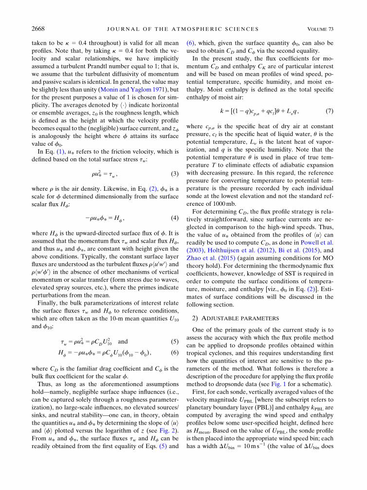
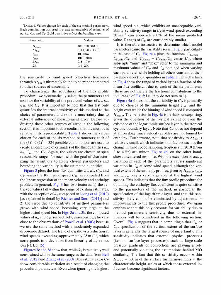
procedure, we systematically select the parameters andmonitor the variability of the predicted values of u*, k*,CD, and CK. It is important to note that this test onlyquantifies the internal sensitivity of this method to thechoice of parameters and not the uncertainty due toexternal influences or measurement error. Before ad-dressing these other sources of error in the followingsection, it is important to first confirm that the method isreliable in its reproducibility. Table 1 shows the valueschosen for each of the six method parameters; each ofthe (3)4 3 (2)2 5 324 possible combinations are used tocreate an ensemble of estimates of the flux quantities u*,k*, CD, and CK. Again, the values are chosen to spanreasonable ranges for each, with the goal of character-izing the sensitivity to freely chosen parameters andbounding the variability in the estimated quantities.Figure 3 plots the four flux quantities u*, k*, CD, and

CK versus the 10-m wind speed U10, as computed fromthe linear regression of the mean velocity and enthalpyprofiles. In general, Fig. 3 has two features: 1) the re-trieved values fall within the range of existing estimates,with the exception of k* compared to Jeong et al. (2012)[as explained in detail by Richter and Stern (2014)] and2) the error due to sensitivity of method parametersgrows with wind speed, becoming very large at thehighest wind speed bin. In Figs. 3a and 3b, the computedvalues of u* andCD, respectively, unsurprisingly lie veryclose to the observations of Powell et al. (2003) becausewe use the same method with a moderately expandeddropsonde dataset. The trend ofCD shows a reduction atwind speeds exceeding approximately 35m s21, whichcorresponds to a deviation from linearity of u* versusU10 [cf. Eq. (5)].Figures 3c and 3d show that, while k* is relatively well

constrained within the same range as the data from Bellet al. (2012) andZhang et al. (2008), the estimates forCK

show considerable variation as a result of changing theprocedural parameters. Even when ignoring the highest

wind speed bin, which exhibits an unacceptable vari-ability, sensitivity ranges inCK at wind speeds exceeding30ms21 can approach 200% of the mean predictedvalue. Ranges of CD are considerably smaller.It is therefore instructive to determine which model

parameters cause the variability seen in Fig. 3, particularlyin the case of CK. Figure 4 plots the fractions jCD,max 2CD,minj/CD and jCK,max 2 CK,minj/CK versus U10, wheresubscripts ‘‘min’’ and ‘‘max’’ refer to the minimum andmaximum values of CD and CK obtained when varyingeach parameter while holding all others constant at theirbaseline values (bold quantities in Table 1). Thus, the linesin Fig. 4 show the range of variability as a fraction of themean flux coefficient due to each of the six parameters(these are not merely the fractional contributions to thetotal range of Fig. 3; i.e., they do not sum to 1).Figure 4a shows that the variability in CD is primarily

due to choices of the minimum height zmin and theheight over which the binning of wind speed is computedHmean. The behavior in Fig. 4a is perhaps unsurprising,given the question of the vertical extent or even theexistence of the logarithmic surface layer in the tropicalcyclone boundary layer. Note that CD does not dependat all on Dkbin since velocity profiles are not binned byenthalpy. Furthermore, note that sensitivity to Dzbin isrelatively small, which indicates that factors such as thechange in wind speed sampling frequency in 2010 (from2 to 4Hz) are minor. Figure 4b, on the other hand,shows a scattered response. With the exception of Dkbin,variation in each of the parameters causes significantvariation in CK at some wind speed, although the ver-tical extent of the enthalpy profiles, given byHmean, zmin,and zmax, play a very large role at the highest windspeeds. This indicates that the flux profile procedure forobtaining the enthalpy flux coefficient is quite sensitiveto the parameters of the method, in particular thespecification of the logarithmic layer, and that this sen-sitivity likely cannot be eliminated by adjustments orimprovements to the flux profile procedure. We againemphasize that this only accounts for variability due tomethod parameters; sensitivity due to external in-fluences will be considered in the following section.Overall, Fig. 4 suggests that in computing either CD orCK, specification of the vertical extent of the surfacelayer is generally the largest source of uncertainty. Thissensitivity indicates that external physical processes(i.e., nonsurface-layer processes), such as large-scalepressure gradients or convection, are playing a roleand potentially violating the assumptions behind MOsimilarity. The fact that this sensitivity occurs withinHmean 5 500m of the surface furthermore hints at thecharacteristic height scales at which these external in-fluences become significant factors.

TABLE 1. Values chosen for each of the six method parameters.Each combination was used to create an ensemble of estimates ofu*, k*, CD, and CK. Bold quantities reflect the baseline case.

Parameter Values

Hmean 100, 250, 500mDkbin 5, 10, 20 kJ kg21

zmin 10, 30mzmax 100, 150mDzbin 2, 5, 10mDu0 0, 1, 2K

JULY 2016 R I CHTER ET AL . 2671

c. Measurement and SST uncertainty

Aside from sensitivity to internal parameters of theflux profile method, estimates of CD and CK are subjectto scatter present in the mean profiles of velocity,moisture, and temperature as well. Furthermore, in thecase of enthalpy, the unknown value of SST, which hasbeen interpolated from 0.258 reanalysis data, remains alarge source of uncertainty as well. In this section a

Monte Carlo–based uncertainty quantification schemewill be used to assess the reliability of the flux co-efficient estimates based on the robustness of thelogarithmic fit through mean profile data as well asvariation in SST.The horizontal error bars in Fig. 2 illustrate the spread

of wind speed data contained within each height andwind speed bin; a similar picture exists for the meanprofiles of enthalpy as well (not shown here). Because

FIG. 3. (a) Friction velocity u*, (b) drag coefficientCD, (c) mean enthalpy profile slope k*, and (d) enthalpy flux coefficientCK obtainedusing the flux profile method. The 10-m wind speed determined by the linear regression through the mean velocity and enthalpy profiles isrepresented by U10. Points and error bars represent the mean and two standard deviations based on the 324-member ensemble withvarying combinations of method parameters. Included are existing observational estimates from the literature.

2672 JOURNAL OF THE ATMOSPHER IC SC IENCES VOLUME 73

the flux profile method depends entirely on the linearregression through the mean values in each height bin,we first consider this regression subject to the 95%confidence interval of each of these mean values. Thebaseline parameters denoted in boldface in Table 1 areused to perform the binning and fitting procedure.Because the regression is performed only on the

mean values—of which there are only O(10) dependingon zmin, zmax, and Dzbin—and not the ‘‘cloud’’ of allavailable velocity/enthalpy measurements, standard lin-ear regression errors can be somewhat misleading. Fora given wind speed and enthalpy bin (i.e., a singlemean profile), we instead use the 95% confidence in-terval of the mean value in each of the height binsto generate a randomly sampled mean value at eachheight, where the confidence interval is given by(hxi2 1:96sx/

ffiffiffiffiffiffiffiffiffiffinsamp

p, hxi1 1:96sx/

ffiffiffiffiffiffiffiffiffiffinsamp

p), where hxi is

the mean value of either wind speed or enthalpy in aparticular height bin, sx is the standard deviation withinthat bin, and nsamp is the number of samples in that bin.For aMonte Carlo sample size of 10000, we then assume anormal distribution of the mean value in each height binwith a standard deviation of 1:96sx/

ffiffiffiffiffiffiffiffiffiffinsamp

p, and compute

u* or k* (i.e., the slope) as the average of all 10 000fitted slopes through the profiles of randomly sampledmean values. This is illustrated in Fig. 5, which for asingle wind speed and enthalpy bin shows the meanenthalpy points at each height z with their 95% con-fidence interval, along with 100 of the 10 000 lines

fitted through randomly sampled mean values (graylines). Each of these individual gray lines has its ownslope k*, and the average value across the entireMonte Carlo ensemble results is shown in the solidblack line.Figure 6 shows the values of u* and k* as a function of

U10, where the error bars now refer to the 10% and 90%quantiles of the 10 000-member ensemble. Compared toFigs. 3a and 3c, the errors associated with the un-certainty of the mean profiles are roughly the same as,perhaps slightly smaller than, the uncertainty associatedwith the parameters of the flux profile method. Again,the uncertainty increases with increasing wind speed,which results primarily from a decreased number ofobservational samples and not necessarily a poorer fit.The uncertainty range in Fig. 6 thus illustrates both thespread in available data within each wind speed andenthalpy bin, as well as the robustness of the linear re-gression. It should be noted that Fig. 6 indicates thatMOtheory may perhaps hold to an appreciable degreewithin tropical cyclones in regions where the wind speedis less than roughly 50m s21, insofar as the existence oflogarithmic mean velocity and enthalpy profiles is proofof this, contrary to Smith and Montgomery (2014). Inother words, we would expect the variability in slopes u*and k* to be much larger if the mean velocity and en-thalpy profiles were not generally logarithmic—a fea-ture suggestive of (but not proof of) the applicability ofMO theory.

FIG. 4. Plots of (a) jCD,max 2 CD,minj/CD and (b) jCK,max 2 CK,minj/CK vs U10, where ‘‘max’’ and ‘‘min’’ refer to the maximum andminimumobtained by varying each of the six parameters outlined in Table 1. See legend for the line associations. Gaps in various curves atthe highest wind speed result from a lack of data, where certain combinations of parameters do not meet the criteria for sample size.

JULY 2016 R I CHTER ET AL . 2673

As noted above and in Richter and Stern (2014), u*and k* are independent of surface conditions, and thusk* is not influenced by uncertainty in SST. The flux co-efficient CK, on the other hand, depends heavily on SSTthrough k0, as shown in Eq. (9). Therefore, for each ofthe 10 000 Monte Carlo members used to compute theensemble ofmean profile regressions, the value of SST isalso sampled from a normal distribution whose meanand standard deviation are equal to the mean andstandard deviation of all interpolated values of SST inthe corresponding wind speed and enthalpy bin. Notethat, because we are using the baseline case, sondeprofiles with Du0 , 2K are excluded from this MonteCarlo procedure, and their inclusion in the analysiswould only work to increase uncertainty beyond what isreported.Figure 7 presents CD and CK versus U10, where again

the symbols refer to the mean of the 10 000-memberensemble and the error bars reflect the 10% and 90%quantile ranges. Included in each panel is a sampleprobability density function (PDF) from the 40–50m s21

wind speed, 350–360kJ kg21 enthalpy bins. The esti-mates ofCD are not in any way sensitive to SST, and thustheir error is only associated with the robustness of theestimate of u*, as determined by the logarithmic fit. Thecomputed values lie very near those of Powell et al.

(2003) and Holthuijsen et al. (2012) because the sameprocedure is used on nearly the same dataset, but moreimportantly the uncertainty range is relatively narrow.Aside from the highest wind speed, estimates of CD

obtained from mean velocity profiles appear to be ac-curate within roughly 50%, taking into account bothprocedural sensitivity (Fig. 3b) and profile variability(Fig. 7a). The PDF included in the inset shows that thedistribution of CD due to variations of u* is indeed rel-atively compact.Estimates of CK, however, are again quite uncertain,

and the mean computed values are only accurate withinroughly 200%. This indicates that, even when excludingsonde profiles where Du0 , 2K, stochastic variability inSST as well as in the mean enthalpy profile leads torelatively large uncertainty in the final value of CK—anuncertainty on the same order as that resulting from theparameter choices outlined in Table 1. The histogramshown in the inset illustrates the heavy tail that occurs inthe PDF of CK, which is indicative of its largeruncertainty.Finally, we should note that additional sources of

uncertainty exist beyond those induced by proceduralparameters, mean profiles, and SST—particularly errorsassociated with instrumentation. We implicitly assumethroughout this analysis that these errors are smallcompared to those outlined above.

3. Simulation data

As an additional test for determining the reliability ofcomputing CD and CK using the flux profile method, weuse a high-resolution large-eddy simulation (LES) of anidealized tropical cyclone to construct ‘‘virtual sondes’’that are transported in time and space through thesimulated vortex. By taking a large number of virtualsonde profiles and subjecting them to an identical pro-cedure as used for the real dropsonde data, we cancompare the computed estimates of CD and CK againstthe surface flux parameterizations that were specified inthe LES code. Moreover, a primary benefit of this test isthat one of the major sources of uncertainty, SST, is nowknown exactly. It should be emphasized that this test ismeant to further determine the ability of the flux profilemethod to recover prescribed surface flux parametersfrom simulated sonde data and not to somehow improvequantitative predictions of CD or CK.We use the Cloud Model 1 (CM1; Bryan and Fritsch

2002; Bryan and Morrison 2012) to simulate an idealizedintense tropical cyclone. CM1 is a three-dimensional, non-hydrostatic, fully compressible cloud model that has beenused to study a wide range of mesoscale and convective-scale phenomena, including tropical cyclones (e.g., Davis

FIG. 5. Sample mean enthalpy profile for the 40–50m s21 windspeed bin, 350–360 kJ kg21 enthalpy bin. Black symbols representmean enthalpy with 95% uncertainty range given by error bars. Solidblack line represents linear regression through mean enthalpy profileusing average value of k* (over all individual Monte Carlo samples).Gray lines represent 100 of the 10 000 Monte Carlo samples usingrandomly sampled mean values, given the 95% uncertainty range.

2674 JOURNAL OF THE ATMOSPHER IC SC IENCES VOLUME 73

2015; Bryan and Morrison 2012). CM1 uses a single do-main and has grid stretching in both the vertical andhorizontal directions in order to maximize resolution inan area of interest while minimizing computational ex-pense. Tropical cyclones are synoptic-scale vortices, so to

contain the entire tropical cyclone within our domain, weuse a 1486km 3 1486km grid, with the model top at25km. To explicitly resolvemost of the large eddies in theboundary layer, we use a horizontal grid spacing of62.5m. It is infeasible and unnecessary to use such fine

FIG. 7. Plots of (a)CD and (b)CK vsU10, where the symbols are the mean of a 10 000-member ensemble, where the SST and the averagevelocity and enthalpy in each height bin are sampled from normal distributions. The error bars denote the 10% and 90% quantiles of theensemble. The insets provide probability density functions for representative bins: the 40–50m s21 wind speed bin and 350–360 kJ kg21

enthalpy bin.

FIG. 6. Plots of (a) u* and (b) k* vsU10, where the symbols refer to the average of the 10 000-memberMonte Carlo ensemble, where themean velocity and enthalpy values in each height bin are randomly sampled according to the 95% confidence interval. The error bars referto the 10% and 90% quantiles of the ensemble.

JULY 2016 R I CHTER ET AL . 2675

resolution over the entire domain. Our area of interest isthe inner-core region, where the eyewall updraft andstrongest winds occur; this is also where most of thesondes within our observational dataset are found.Therefore, we use constant 62.5-mhorizontal grid spacingin an 80km3 80km box centered on the vortex, which issufficient to cover the entire inner-core region.Outside ofthis box, the horizontal grid spacing stretches to 15km bythe outer boundary. In the lowest 3km, vertical gridspacing is constant at 31.25m (half of the horizontal) andstretches to 500m near the model top.We simulate our storm on an f plane, in a quiescent

environment (no mean flow), and over a homogeneousand fixed SST of 288C. The initial atmospheric envi-ronment is horizontally homogeneous, using theDunion(2011) ‘‘moist tropical’’ mean sounding. We insert abalanced, weak vortex into this environment, with initialmaximum winds of 20m s21. For microphysics, we usethe Morrison double-moment scheme (Bryan andMorrison 2012), and we do not parameterize either ra-diation or convection. Outside of the fine-mesh region,turbulence is entirely unresolved and must be parame-terized; for this, we use the turbulence scheme of Bryanand Rotunno (2009). Inside of the fine-mesh region, weturn this parameterization off and only use an LESsubgrid model based on that of Deardorff (1980).Tropical cyclones typically intensify over a period of

several days, and even with the grid stretching in CM1, itremains impractical to run our simulation for such a pe-riod (there are 16643 16643 160 grid points). Therefore,we first spin up a tropical cyclone in an axisymmetricversion ofCM1 and use the time-averagedoutput from 72to 84h, when the tropical cyclone is approximately cate-gory 5, to initialize the LES. We then integrate theLES for only 2h. Though this may seem short, three-dimensional turbulence develops within only 10min, andthe turbulence is statistically steady after an hour (notshown). In a future publication, we will present this andother such simulations in much greater detail.To emulate dropsondes within the simulation, we cal-

culate parcel trajectories that we modify by adding a fallspeed.Weuse the exact samedensity-dependent fall speedformulation that is used in ASPEN for the observedsondes. These virtual dropsonde trajectories are integratedwithin the model using a second-order Runge–Kuttascheme. For the results presented below, we releasedsondes in a 20km 3 20km box that covers the southwestquadrant of the simulated tropical cyclone (TC). Sondesare placed at 62.5-m intervals horizontally (i.e., at everymodel grid point), and in total there are 103041 virtualsondes. The initial height of all sondes is 2500m, which is atypical release height for observed sondes. Recall that theobserved sondes sample two or four times per second; in

order to minimize storage space, we output virtual sondedata only every 3 s. As each virtual sonde samples slightlydifferent heights because of differences in vertical veloci-ties (of the air) and as we are bin averaging the profiles,this difference in sampling rate between the observed andvirtual sondes should not substantially affect our results.The sondes are all released at t5 2h, and their trajectoriesare integrated for 10min, which is enough time for almostall of the sondes to fall to the surface.For estimating CD and CK from the virtual sonde pro-

files, the exact same procedure outlined in section 2a isused, but now the parameter Du0 is not needed becausethere is only a single known value of SST. Once again thereliability of this method is evaluated based on the sensi-tivity of CD and CK to method parameters. Table 2 isanalogous to Table 1 and shows the values chosen forHmean,Dkbin, zmin, zmax, andDzbin used in the virtual sondeanalysis. Note that zmin andDkbin both deviate slightly fromthe previous case because of restrictions of the computa-tional grid and choice of boundary conditions, respectively.Figure 8 showsCD andCK computed from the 103 041

virtual sonde profiles from a single storm using the fluxprofile method. As with the real sondes, internal vari-ability of CK due to method parameters is much largerthan that associated withCD. Predictions of bothCD andCK lie in the general proximity of the prescribed values(given by the solid blue lines), particularly at the highestwind speeds. Between wind speeds of 20 and 40m s21,however, bothCD andCK underpredict the true value byover 100% (i.e., by a factor of 2).While this test is of course limited by the accuracy of

the turbulence generated by the simulation, it onceagain confirms that the flux profile method is able toprovide estimates of flux coefficients that lie in the cor-rect general range but that are limited in their quanti-tative calculation. It is worthwhile to caution that purelynumerical aspects, such as the vertical grid resolutionand details of the LES subgrid model, can and do in-fluence the calculation of CD and CK using the virtualsonde approach (not shown). While these factors areunavoidable, we argue that they are small enough thatvaluable insight can be gained into the validity and ro-bustness of the flux profile method.

TABLE 2. Values chosen for each of the method parameters forthe virtual sonde experiments. Each combination was used tocreate an ensemble of estimates of CD and CK.

Parameter Values

Hmean 100, 250, 500mDkbin 2, 5, 10 kJ kg21

zmin 20, 50mzmax 100, 150mDzbin 2, 5, 10m

2676 JOURNAL OF THE ATMOSPHER IC SC IENCES VOLUME 73

4. Discussion

Given the above results for both the real and simu-lated sonde profiles, two specific points merit furtherdiscussion. The first is regarding the agreement (or lackthereof) between the virtual sonde predictions of thesurface flux coefficients and the prescribed values shownin Fig. 8. The other is regarding the relationship betweenCK and its sensible and latent heat counterparts CH andCE, since these are typically the values of practical in-terest in numerical weather prediction models.

a. Radius dependence

In section 3, virtual sonde trajectories in a turbulence-resolving LES were used to test the flux profile methodunder conditions where both the SST and the actualsurface flux parameterizations are known exactly.Figure 8 indicated that the mean values obtained by theflux profile method agreed qualitatively with real sondedata but underestimated the prescribed values some-what, particularly at lower wind speeds.Under conditions where the mean profiles of various

quantities are not determined exclusively by the surfaceflux and the height above the surface (i.e., the underlyingbasis of MO theory), the existence of a logarithmic layermay be called into question, particularly one that ex-tends an appreciable distance upward from the oceansurface. One such violation is discussed in detail bySmith and Montgomery (2014), who argue that radial

pressure balances near the eye of the tropical cycloneviolate the underlying assumptions behind the existenceof a logarithmic velocity profile.We therefore perform a simple test to determine

what, if any, sensitivity the flux profile predictions of CD

and CK have to rsonde, the distance from the simulatedstorm center at which the virtual sonde is released. InFig. 9, two curves of CD and CK are provided: one usingsondes in the range 0, rsonde, 10km and the other onlyusing sondes in the range 10 , rsonde , 20km. For thissimulated storm, the radius of maximum wind near thesurface is approximately 12 km.It is clear from Fig. 9 that proximity to the storm

center indeed significantly changes the prediction of thesurface flux coefficients via the flux profile method. Forthe range 0 , rsonde , 10km, both CD and CK severelyunderpredict the prescribed values, while for the range10 , rsonde , 20km the estimated mean values are inclose agreement with the prescribed values. In this case,however (Figs. 9c,d), a large degree of uncertaintycontinues to exist, particularly for CK, as given by thevariability resulting from changing the parameters of themethod (see discussion in section 3).Figure 9 would therefore suggest that the flux profile

method is inappropriate in regions near the tropicalcyclone eye and could possibly lead to underpredictionsof CD and CK if these sonde profiles are included in theflux profile analysis, perhaps for reasons given by Smithand Montgomery (2014). Another possibility is that we

FIG. 8. Plots of (a) CD and (b) CK vs U10 as estimated from the virtual sonde data. The solid blue lines correspond to the prescribedsurface flux coefficients in the code. The error bars reflect two standard deviations from the mean of the (3)3 3 (2)2 5 108-memberensemble based on the combinations of parameters in Table 2.

JULY 2016 R I CHTER ET AL . 2677

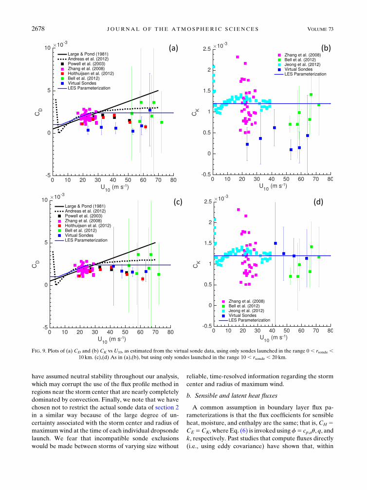
have assumed neutral stability throughout our analysis,which may corrupt the use of the flux profile method inregions near the storm center that are nearly completelydominated by convection. Finally, we note that we havechosen not to restrict the actual sonde data of section 2in a similar way because of the large degree of un-certainty associated with the storm center and radius ofmaximumwind at the time of each individual dropsondelaunch. We fear that incompatible sonde exclusionswould be made between storms of varying size without

reliable, time-resolved information regarding the stormcenter and radius of maximum wind.

b. Sensible and latent heat fluxes

A common assumption in boundary layer flux pa-rameterizations is that the flux coefficients for sensibleheat, moisture, and enthalpy are the same; that is, CH 5CE5CK, where Eq. (6) is invoked usingf5 cp,au, q, andk, respectively. Past studies that compute fluxes directly(i.e., using eddy covariance) have shown that, within

FIG. 9. Plots of (a) CD and (b) CK vs U10, as estimated from the virtual sonde data, using only sondes launched in the range 0 , rsonde ,10 km. (c),(d) As in (a),(b), but using only sondes launched in the range 10 , rsonde , 20 km.

2678 JOURNAL OF THE ATMOSPHER IC SC IENCES VOLUME 73

uncertainty, this relationship holds true (DeCosmo et al.1996; Drennan et al. 2007; Zhang et al. 2008). In thecurrent context, we noted above that one of the re-quirements of MO theory is that there exist no elevatedsources of the quantity of interest, including those due toevaporation/condensation. Thus, instead of computingfluxes of heat and moisture separately (which are po-tentially influenced by evaporation and condensation ofrain and/or spray), we have focused so far primarily onthe flux of moist enthalpy k, since it is conserved duringphase transitions and therefore does not violate this MOcriterion.It is worthwhile to comment, however, on the pre-

dictions of latent and sensible heat flux as computed bythe flux profile method using the observational (i.e., notthe virtual) dropsonde dataset. The procedure outlinedin section 2 can be used on mean profiles of temperatureand moisture, in conjunction with Eq. (6), to computeestimates of surface fluxes of sensible and latent heatover all 37 tropical cyclones:

HS52rc

p,au*u* (10)

and

HL52r(L

y1 c

p,luSST)u*q*, (11)

respectively, where u* and q* are computed via theslopes of the mean temperature and moisture profiles,

and uSST is a mean SST, which we have crudely esti-mated to be 300K (this term is overwhelmed by the la-tent heat of vaporization).Figure 10a shows HS and HL as a function of U10,

along with the enthalpy flux as computed by HK 52ru*k* for the real sonde data. Also shown is thesum ofHS andHL, which should ideally sum to exactlyHK. Discrepancies between HK and HS 1 HL arelikely due to violations of MO assumptions inducedby evaporating/condensing rainfall or spray withinthe lower boundary layer, thus making neither temper-ature nor moisture a conserved quantity. Figure 10ashows a close agreement between the two, suggestingthat nonconservative effects may be small. Figure 10aillustrates that latent heat overwhelmingly dominates thetotal enthalpy flux, somewhat unsurprisingly, and thatthe sensible heat flux, as computed by this method, isslightly negative.If the flux coefficients CH and CE are computed,

however, (Fig. 10b), the values of CH are actually neg-ative, suggesting that sensible heat is being transportedcountergradient according to Eq. (6). This is likely un-physical and results from a combination of small-in-magnitude sensible heat fluxes and highly uncertainvalues of SST. The values of CE, on the other hand, arequite similar to the values of CK. Therefore, in this case,the relationship CE 5 CK seems plausible (within un-certainty) but cannot be confirmed or refuted for CH

FIG. 10. (a) The fluxes of enthalpy, sensible heat, and latent heat as computed byEq. (6). The sumof the latent and sensible heat is shownas well, which should ideally match the enthalpy flux as computed via k* and u*, given perfect adherence to MO theory. (b) The sensibleheat and water vapor flux coefficients CH and CE, respectively, as a function of U10.

JULY 2016 R I CHTER ET AL . 2679

because of what is essentially a large signal-to-noiseratio of sensible heat flux to unknown SST values.

5. Conclusions

Dropsonde data recorded across 37 different tropicalcyclones were used to construct mean profiles of windspeed and enthalpy in order to use MO theory and theflux profile method to estimate surface fluxes and surfaceflux coefficients. Of primary interest in this study is thereliability of this method when subjected to variability inthe internal parameters of the method (i.e., binning pro-cedures, threshold values, etc.), scatter among individualprofiles and the robustness of the linear regression throughtheirmean, anduncertainty in theSSTestimate. In addition,a high-resolution large-eddy simulation of an idealizedtropical cyclone vortex was used to further validate thisprocedure by constructing simulated sonde profiles fromthe simulation and performing an identical retrieval ofsurface flux coefficients. In this case, the value of SST isknownexactly, and the estimated values ofCD andCKwerecompared to the prescribed values in the numerical code.Overall, the results show that estimates of CD using

dropsonde data, as done by Powell et al. (2003) andHolthuijsen et al. (2012), are accurate to within ap-proximately 50% up to wind speeds of roughly 50ms21.This includes the sensitivity of this method to regressionprocedures as well as its ability to quantitatively recoverprescribed surface values in the numerical simulations.While a relative error of 50% could be consideredsomewhat large, it does not preclude one from using theflux profile method estimates of CD to confirm qualita-tive conclusions about the behavior of the drag co-efficient at high winds.For computing CK, on the other hand, this analysis

shows that, while the estimated values lie in the samegeneral range as others in the literature (Zhang et al.2008; Bell et al. 2012; Jeong et al. 2012), variability of theestimated values is relatively high, restricting a quanti-tative prediction to only within 200%. The uncertaintyin SST is a major source of this variability, but inherentsensitivity in the binning procedure leads to large spreadas well, limiting the ability of the flux profile method topredict surface flux coefficients even if SST weresomehow known. Beyond this, violations of MO theory,particularly near the tropical cyclone eye, potentiallycorrupt the predictions of both CD and CK; likewise,other factors, such as neglecting surface currents in thecomputation of CD, may impact the accuracy as well.The flux profile technique thus provides a means of

roughly estimating quantities such as CD and CK, how-ever with limited quantitative skill. While it may guidequalitative considerations, such as whether or not the

value of CD saturates (Powell et al. 2003) or whether ornot spray influences enthalpy fluxes (Richter and Stern2014), its use as a tool for refining values of CD or CK isnot recommended. If one were interested in the surfacefluxes themselves (as opposed to the flux coefficients),knowledge of SST and other surface conditions is notrequired, and predictions via the flux profile method arequite robust (assuming conditions for MO theory hold);however, these quantities are of much less practical usefor universal surface flux parameterizations.

Acknowledgments. The authors would like to acknowl-edge the National Oceanic and Atmospheric Adminis-tration’s Hurricane Research Division for making thedropsonde data used in this study publicly available. Theauthors would also like to thank George Bryan forhelpful discussions, as well as three reviewers who helpedimprove the quality of the manuscript.

REFERENCES

Andreas, E. L, 2004: Spray stress revisited. J. Phys. Oceanogr., 34,1429–1440, doi:10.1175/1520-0485(2004)034,1429:SSR.2.0.CO;2.

——, 2010: Spray-mediated enthalpy flux to the atmosphere andsalt flux to the ocean in highwinds. J. Phys. Oceanogr., 40, 608–619, doi:10.1175/2009JPO4232.1.

——, 2011: Fallacies of the enthalpy transfer coefficient over theocean in high winds. J. Atmos. Sci., 68, 1435–1445, doi:10.1175/2011JAS3714.1.

Bao, J.-W., C. W. Fairall, S. A. Michelson, and L. Bianco, 2011:Parameterizations of sea-spray impact on the air–sea mo-mentum and heat fluxes. Mon. Wea. Rev., 139, 3781–3797,doi:10.1175/MWR-D-11-00007.1.

Bell, M. M., M. T. Montgomery, and K. A. Emanuel, 2012: Air–seaenthalpy and momentum exchange at major hurricane windspeeds observed during CBLAST. J. Atmos. Sci., 69, 3197–3222, doi:10.1175/JAS-D-11-0276.1.

Bi, X., and Coauthors, 2015: Observed drag coefficients in highwinds in the near offshore of the South China Sea. J. Geophys.Res. Atmos., 120, 6444–6459, doi:10.1002/2015JD023172.

Black, P. G., and Coauthors, 2007: Air–sea exchange in hurricanes:Synthesis of observations from the Coupled Boundary LayerAir–Sea Transfer experiment. Bull. Amer. Meteor. Soc., 88,357–374, doi:10.1175/BAMS-88-3-357.

Bryan, G. H., 2012: Effects of surface exchange coefficients andturbulence length scales on the intensity and structure of nu-merically simulated hurricanes. Mon. Wea. Rev., 140, 1125–1143, doi:10.1175/MWR-D-11-00231.1.

——, 2013: Comments on sensitivity of tropical-cyclone models tothe surface drag coefficient. Quart. J. Roy. Meteor. Soc., 139,1957–1960, doi:10.1002/qj.2066.

——, and J. M. Fritsch, 2002: A benchmark simulation for moist non-hydrostatic numerical models. Mon. Wea. Rev., 130, 2917–2928,doi:10.1175/1520-0493(2002)130,2917:ABSFMN.2.0.CO;2.

——, and R. Rotunno, 2009: The maximum intensity of tropicalcyclones in axisymmetric numerical model simulations. Mon.Wea. Rev., 137, 1770–1789, doi:10.1175/2008MWR2709.1.

——, and H. Morrison, 2012: Sensitivity of a simulated squallline to horizontal resolution and parameterization of

2680 JOURNAL OF THE ATMOSPHER IC SC IENCES VOLUME 73

microphysics. Mon. Wea. Rev., 140, 202–225, doi:10.1175/MWR-D-11-00046.1.

D’Asaro, E. A., and Coauthors, 2013: Impact of typhoons on theocean in the Pacific. Bull. Amer. Meteor. Soc., 95, 1405–1418,doi:10.1175/BAMS-D-12-00104.1.

Davis, C., 2015: The formation of moist vortices and tropical cy-clones in idealized simulations. J. Atmos. Sci., 72, 3499–3516,doi:10.1175/JAS-D-15-0027.1.

Deardorff, J.W., 1980: Stratocumulus-cappedmixed layers derivedfrom a three-dimensional model. Bound.-Layer Meteor., 18,495–527, doi:10.1007/BF00119502.

DeCosmo, J., K. B. Katsaros, S. D. Smith, R. J. Anderson, W. A.Oost, K. Bumke, and H. Chadwick, 1996: Air–sea exchange ofwater vapor and sensible heat: The Humidity Exchange overthe Sea (HEXOS) results. J. Geophys. Res., 101, 12 001–12 016, doi:10.1029/95JC03796.

Dingman, S. L., 2008:Physical Hydrology. 2nd ed.Waveland Press,646 pp.

Donelan,M.A., B. K.Haus, N.Reul,W. J. Plant, M. Stiassnie, H. C.Graber, O. B. Brown, and E. S. Saltzman, 2004: On the limitingaerodynamic roughness of the ocean in very strong winds.Geophys. Res. Lett., 31, L18306, doi:10.1029/2004GL019460.

Drennan, W. M., J. A. Zhang, J. R. French, C. McCormick, andP. G. Black, 2007: Turbulent fluxes in the hurricane boundarylayer. Part II: Latent heat flux. J. Atmos. Sci., 64, 1103–1115,doi:10.1175/JAS3889.1.

Dunion, J. P., 2011: Rewriting the climatology of the tropical NorthAtlantic and Caribbean Sea atmosphere. J. Climate, 24, 893–908, doi:10.1175/2010JCLI3496.1.

Edson, J. B., and Coauthors, 2013: On the exchange of momentumover the open ocean. J. Phys. Oceanogr., 43, 1589–1610,doi:10.1175/JPO-D-12-0173.1.

Emanuel, K. A., 1986: An air–sea interaction theory for tropical cy-clones. Part I: Steady-state maintenance. J. Atmos. Sci., 43, 585–605, doi:10.1175/1520-0469(1986)043,0585:AASITF.2.0.CO;2.

——, 1995: Sensitivity of tropical cyclones to surface exchangecoefficients and a revised steady-state model incorporatingeye dynamics. J. Atmos. Sci., 52, 3969–3976, doi:10.1175/1520-0469(1995)052,3969:SOTCTS.2.0.CO;2.

Fairall, C. W., J. D. Kepert, and G. J. Holland, 1994: The effect ofsea spray on surface energy transports over the ocean.GlobalAtmos. Ocean Syst., 2, 121–142.

——, E. F. Bradley, J. E. Hare, A. A. Grachev, and J. B. Edson,2003: Bulk parameterization of air–sea fluxes: Updates andverification for the COARE algorithm. J. Climate, 16, 571–591,doi:10.1175/1520-0442(2003)016,0571:BPOASF.2.0.CO;2.

French, J. R., W. M. Drennan, J. A. Zhang, and P. G. Black, 2007:Turbulent fluxes in the hurricane boundary layer. Part I: Mo-mentumflux. J.Atmos. Sci.,64, 1089–1102, doi:10.1175/JAS3887.1.

Green, B. W., and F. Zhang, 2013: Impacts of air–sea flux parameter-izations on the intensity and structure of tropical cyclones. Mon.Wea. Rev., 141, 2308–2324, doi:10.1175/MWR-D-12-00274.1.

——, and ——, 2014: Sensitivity of tropical cyclone simulations toparametric uncertainties in air–sea fluxes and implications forparameter estimation. Mon. Wea. Rev., 142, 2290–2308,doi:10.1175/MWR-D-13-00208.1.

Haus, B. K., D. Jeong,M.A.Donelan, J. A. Zhang, and I. Savelyev,2010: Relative rates of sea–air heat transfer and frictional dragin very high winds. Geophys. Res. Lett., 37, L07802, doi:10.1029/2009GL042206.

Hock, T. F., and J. L. Franklin, 1999: The NCAR GPS dropwind-sonde. Bull. Amer. Meteor. Soc., 80, 407–420, doi:10.1175/1520-0477(1999)080,0407:TNGD.2.0.CO;2.

Holthuijsen, L. H., M. D. Powell, and J. D. Pietrzak, 2012: Windand waves in extreme hurricanes. J. Geophys. Res., 117,C09003, doi:10.1029/2012JC007983.

Jarosz, E., D. A. Mitchell, D. W. Wang, and W. J. Teague, 2007:Bottom-up determination of air–sea momentum exchangeunder a major tropical cyclone. Science, 315, 1707–1709,doi:10.1126/science.1136466.

Jeong, D., B. K. Haus, andM. A. Donelan, 2012: Enthalpy transferacross the air–water interface in high winds including spray.J. Atmos. Sci., 69, 2733–2748, doi:10.1175/JAS-D-11-0260.1.

Kudryavtsev, V. N., and V. K. Makin, 2007: Aerodynamic rough-ness of the sea surface at high winds. Bound.-Layer Meteor.,125, 289–303, doi:10.1007/s10546-007-9184-7.

Makin, V. K., 2005: A note on the drag of the sea surface at hur-ricane winds. Bound.-Layer Meteor., 115, 169–176, doi:10.1007/s10546-004-3647-x.

Mangarella, P. A., A. J. Chambers, R. L. Street, and E. Y. Hsu, 1973:Laboratory studies of evaporation and energy transfer througha wavy air–water interface. J. Phys. Oceanogr., 3, 93–101,doi:10.1175/1520-0485(1973)003,0093:LSOEAE.2.0.CO;2.

Monin, A. S., and A. M. Yaglom, 1971: Statistical Fluid Mechanics.Vol. 1. Dover Publications, 769 pp.

Montgomery, M. T., R. K. Smith, and S. V. Nguyen, 2010:Sensitivity of tropical-cyclone models to the surface dragcoefficient. Quart. J. Roy. Meteor. Soc., 136, 1945–1953,doi:10.1002/qj.702.

Mueller, J. A., and F. Veron, 2014: Impact of sea spray on air–seafluxes. Part II: Feedback effects. J. Phys. Oceanogr., 44, 2835–2853, doi:10.1175/JPO-D-13-0246.1.

Potter, H., H. C. Graber, N. J.Williams, C. O. Collins, R. J. Ramos,and W. M. Drennan, 2015: In situ measurements of momen-tum fluxes in typhoons. J. Atmos. Sci., 72, 104–118, doi:10.1175/JAS-D-14-0025.1.

Powell, M. D., P. J. Vickery, and T. A. Reinhold, 2003: Reduceddrag coefficient for high wind speeds in tropical cyclones.Nature, 422, 279–283, doi:10.1038/nature01481.

Reichl, B. G., T. Hara, and I. Ginis, 2014: Sea state dependence ofthe wind stress over the ocean under hurricane winds. J. Geophys.Res. Oceans, 119, 30–51, doi:10.1002/2013JC009289.

Reynolds, R. W., T. M. Smith, C. Liu, D. B. Chelton, K. S. Casey,and M. G. Schlax, 2007: Daily high-resolution-blended ana-lyses for sea surface temperature. J. Climate, 20, 5473–5496,doi:10.1175/2007JCLI1824.1.

Richter, D. H., and D. P. Stern, 2014: Evidence of spray-mediatedair–sea enthalpy flux within tropical cyclones. Geophys. Res.Lett., 41, 2997–3003, doi:10.1002/2014GL059746.

Rios-Berrios, R., T. Vukicevic, and B. Tang, 2014: Adopting modeluncertainties for tropical cyclone intensity prediction. Mon.Wea. Rev., 142, 72–78, doi:10.1175/MWR-D-13-00186.1.

Rosenthal, S. L., 1971: The response of a tropical cyclone modelto variations in boundary layer parameters, initial condi-tions, lateral boundary conditions, and domain size. Mon.Wea. Rev., 99, 767–777, doi:10.1175/1520-0493(1971)099,0767:TROATC.2.3.CO;2.

Smith, R. K., andM. T. Montgomery, 2014: On the existence of thelogarithmic surface layer in the inner core of hurricanes.Quart. J. Roy. Meteor. Soc., 140, 72–81, doi:10.1002/qj.2121.

Sraj, I., and Coauthors, 2013: Bayesian inference of drag parame-ters using AXBT data from Typhoon Fanapi.Mon. Wea. Rev.,141, 2347–2367, doi:10.1175/MWR-D-12-00228.1.

Sullivan, P. P., and J. C. McWilliams, 2010: Dynamics of winds andcurrents coupled to surface waves.Annu. Rev. FluidMech., 42,19–42, doi:10.1146/annurev-fluid-121108-145541.

JULY 2016 R I CHTER ET AL . 2681

Takagaki, N., S. Komori, N. Suzuki, K. Iwano, T. Kuramoto,S. Shimada, R. Kurose, and K. Takahashi, 2012: Strong cor-relation between the drag coefficient and the shape of thewindsea spectrum over a broad range of wind speeds. Geophys.Res. Lett., 39, L23604, doi:10.1029/2012GL053988.

Troitskaya, Y. I., D.A. Sergeev, A.A.Kandaurov, G.A. Baidakov,M. A. Vdovin, and V. I. Kazakov, 2012: Laboratory and the-oretical modeling of air–sea momentum transfer under severewind conditions. J. Geophys. Res., 117, C00J21, doi:10.1029/2011JC007778.

Veron, F., 2015: Ocean spray.Annu. Rev. FluidMech., 47, 507–538,doi:10.1146/annurev-fluid-010814-014651.

Vickers, D., L. Mahrt, and E. L Andreas, 2013: Estimates of the10-m neutral sea surface drag coefficient from aircraft eddy-covariance measurements. J. Phys. Oceanogr., 43, 301–310,doi:10.1175/JPO-D-12-0101.1.

Zhang, J. A., P. G. Black, J. R. French, and W. M. Drennan, 2008:First direct measurements of enthalpy flux in the hurricaneboundary layer: The CBLAST results.Geophys. Res. Lett., 35,L14813, doi:10.1029/2008GL034374.

Zhao, Z.-K., C.-X. Liu, Q. Li, G.-F. Dai, Q.-T. Song, and W.-H.Lv, 2015: Typhoon air–sea drag coefficient in coastal re-gions. J. Geophys. Res. Oceans, 120, 716–727, doi:10.1002/2014JC010283.

2682 JOURNAL OF THE ATMOSPHER IC SC IENCES VOLUME 73