AN ASSESSMENT OF THE ECONOMIC IMPACT - document search

Economic Commission for Latin America and the Caribbean

Subregional Headquarters for the Caribbean

AN ASSESSMENT OF THE ECONOMIC IMPACT OF CLIMATE CHANGE ON THE AGRICULTURE SECTOR IN JAMAICA

__________

This document has been reproduced without formal editing.

LIMITED

LC/CAR/L.324

22 October 2011

ORIGINAL: ENGLISH

i

Notes and explanations of symbols: The following symbols have been used in this study: A full stop (.) is used to indicate decimals The use of a hyphen (-) between years, for example, 2010-2019, signifies an annual average for the calendar years involved, including the beginning and ending years, unless otherwise specified. The word “dollar” refers to United States dollars, unless otherwise specified. N.d. refers to forthcoming material with no set publication date. The boundaries and names shown and the designations used on maps do not imply official endorsement or acceptance by the United Nations.

ii

Acknowledgement

The Economic Commission for Latin America and the Caribbean (ECLAC) Subregional Headquarters for the Caribbean, wishes to acknowledge the assistance of Michael Witter, consultant, in the preparation of

this report.

iii

Table of contents

Notes and explanations of symbols: .................................................................................................. i I. INTRODUCTION AND BACKGROUND...................................................................................... 1 II. LITERATURE REVIEW ................................................................................................................ 1

A. MODELS FOR ECONOMIC ANALYSIS....................................................................................... 2 1. Production Function Model.......................................................................................................... 2 2. Ricardian Model .......................................................................................................................... 2 3. Agronomic-Economic/Crop Growth Model.................................................................................. 3 4. Agro-Ecological Zones (AEZ) (Land Zone Models)..................................................................... 4 5. Integrated Impact Assessment Models (IAMs) ............................................................................. 4

B. CHOICE OF METHODOLOGY ..................................................................................................... 6 C. CHOICE OF CROPS....................................................................................................................... 6

III. THE AGRICULTURAL SECTOR IN JAMAICA ....................................................................... 7 A. RURAL SOCIAL STRUCTURE..................................................................................................... 7

1. Population ................................................................................................................................... 7 2. Migration..................................................................................................................................... 9 3. Ageing......................................................................................................................................... 9 4. Poverty ...................................................................................................................................... 10

B. RURAL ECONOMIC STRUCTURE ............................................................................................ 10 1. Employment .............................................................................................................................. 11 2. Water......................................................................................................................................... 12 3. Output of Agriculture, Forestry and Fishing ............................................................................... 13 4. Contribution to GDP.................................................................................................................. 14 5. Livestock................................................................................................................................... 15 6. Beef and Poultry ........................................................................................................................ 17 7. Forestry ..................................................................................................................................... 18 8. Fishing....................................................................................................................................... 19

C. EXPORT AGRICULTURE........................................................................................................... 20 1. Sugar cane ................................................................................................................................. 20 2. Citrus......................................................................................................................................... 22 3. Bananas ..................................................................................................................................... 22 4. Coffee........................................................................................................................................ 22

D. DOMESTIC CROPS..................................................................................................................... 23 E. VULNERABILITY....................................................................................................................... 23 F. PROJECTIONS............................................................................................................................. 24

IV. ESTIMATING THE IMPACT OF CLIMATE CHANGE .......................................................... 24 A. CLIMATE CHANGE SCENARIOS.............................................................................................. 24 B. THE APPROACH......................................................................................................................... 27

1. Modelling the yield of Sugar cane.............................................................................................. 28 2. Forecasts.................................................................................................................................... 31 3. Forecast Statistics for Sugar Cane .............................................................................................. 33 4. Adaptation ................................................................................................................................. 33

iv

5. Modelling the yield of Yellow Yam ........................................................................................... 33 6. Forecast Statistics for Yam......................................................................................................... 37 7. Modelling the yield of Escallion................................................................................................. 38 8. Forecasts.................................................................................................................................... 39 9. Forecast Statistics for Escallion.................................................................................................. 40

C. OTHER IMPACTS ON THE WIDER AGRICULTURAL SECTOR.............................................. 40 1. Sea level rise.............................................................................................................................. 41 2. Flooding .................................................................................................................................... 42 3. Drought ..................................................................................................................................... 42 4. Hurricanes ................................................................................................................................. 42

V. ADAPTATION ............................................................................................................................. 43 A. INSURANCE ............................................................................................................................... 43

1. Sugar cane ................................................................................................................................. 49 2. Yam........................................................................................................................................... 50 3. Escallion.................................................................................................................................... 52

VI. CONCLUSIONS AND RECOMMENDATIONS ...................................................................... 56 REFERENCES...................................................................................................................................... 58

v

List of tables Table 1: Net Benefit = Avoided loss under each Scenario minus Cost of adaptation, US$ million, at different discount rates ........................................................................................................................... ix Table 2: Population indicators ................................................................................................................. 8 Table 3: Farm Size Group in Hectares .................................................................................................. 11 Table 4: Area in Farming in Jamaica 1996, 2000, 2007.......................................................................... 11 Table 5: Water Consumption by Sector.................................................................................................. 13 Table 6: Profile of Dairy Farms in Jamaica ............................................................................................ 17 Table 7: Agriculture Sector Plan- Proposed Outcome Indicators ............................................................ 24 Table 8: Unit Root Tests........................................................................................................................ 30 Table 9: Factors determining the Yield of Sugar Cane per year in tonnes per hectare............................. 31 Table 10: Forecast Statistics for the Sugar Cane model .......................................................................... 33 Table 11: Unit Root Tests...................................................................................................................... 34 Table 12: Factors determining Yield of Yellow Yam per year in tonnes per hectare .............................. 35 Table 13: Forecast Statistics for the Yam model .................................................................................... 37 Table 14: Unit Root Test ....................................................................................................................... 38 Table 15: Factors determining the Yield of Escallion per year in tonnes per hectare ............................... 39 Table 16: Forecast Statistics for the Escallion model.............................................................................. 40 Table 17: Estimates of Hurricane Damage to Agriculture....................................................................... 43 Table 18: Comparative Costs of No Adaptation vs Net Benefits of Adaptation, 2012-2050 – Sugar Cane, US$ millions ......................................................................................................................................... 50 Table 19: Comparative Costs of No Adaptation vs Net Benefits of Adaptation, 2012-2050 – Sugar Cane, as a percentage of GDP in 2008 ............................................................................................................. 50 Table 20: Comparative Costs of No Adaptation vs Net Benefits of Adaptation, 2012-2050 – Yam, US$ millions ................................................................................................................................................. 51 Table 21: Comparative Costs of No Adaptation vs Net Benefits of Adaptation, 2012-2050 – Yam, as a percentage of GDP in 2008.................................................................................................................... 52 Table 22: Comparative Cost of Adaptation vs No Adaptation – Escallion .............................................. 53 Table 23: Comparative Costs of No Adaptation vs Net Benefits of Adaptation, 2012-2050 – Escallion, as a percentage of GDP in 2008 ................................................................................................................. 53 Table 24: Comparative Costs of No Adaptation vs Net Benefits of Adaptation, 2012-2050 – Sugar cane, Yam, and Escallion, as a percentage of GDP in 2008 ............................................................................. 53 Table 25: Net Benefit = Avoided loss under A2 minus Cost of adaptation, US$ million, at discount rate 54 Table 26: Return on Investment in Adaptation ....................................................................................... 55 Table 27: Net Benefit = Avoided loss under each Scenario minus Cost of adaptation, US$ million, at discount rate.......................................................................................................................................... 56

I.

vi

List of figures Figure 1: Integrated Impact Assessment Model........................................................................................ 5 Figure 2: Average annual growth rate of the population for the previous decade (%)................................ 8 Figure 3: Rural Population as a percentage of total population (%)........................................................... 9 Figure 4: Agriculture, Forestry, Fishing: % of total employment ............................................................ 12 Figure 5: Production Index - Agriculture, Livestock, Gross per capita.................................................... 13 Figure 6: Contribution of Total Agriculture, Export Agriculture and Domestic Agriculture to GDP....... 14 Figure 7: Contribution to GDP- Domestic Agriculture, Root Crops........................................................ 15 Figure 8: Contribution of total exports of agriculture and sugar cane to GDP ......................................... 15 Figure 9: Contribution to GDP - Livestock, Forestry, Fishing, % ........................................................... 16 Figure 10: Milk output, million litres, 1969-2009................................................................................... 16 Figure 11: Index of poultry and livestock production ............................................................................. 18 Figure 12: Fish Production, tonnes......................................................................................................... 20 Figure 13: Sugar production (1978- 2007) ............................................................................................. 21 Figure 14: ECHAM A2, maximum, mean, minimum temperature (0C)................................................... 25 Figure 15: ECHAM B2 Maximum, Mean, Minimum Temperature, °C .................................................. 26 Figure 16: ECHAM A2, B2 mean temperature, °C................................................................................. 26 Figure 17: ECHAM A2, B2 Precipitation, mm....................................................................................... 27 Figure 18: Rainfall and the Sugar Cane Cycle........................................................................................ 31 Figure 19: Projected Average Sugar Cane Yield, tonnes per Hectare 2011-2050 .................................... 32 Figure 20: Rainfall and the yield of yellow yam..................................................................................... 36 Figure 21: Projected Average Yellow Yam Yield, tonnes/ha, 2011-2050 ............................................... 37 Figure 22: Projected Average Escallion Yield (tonnes per hectare), 2011-2050 ..................................... 40 Figure 23: Contaminated Aquifers ......................................................................................................... 42

vii

List of Acronyms 1. AEZ – Agro-Ecological Zones 2. CC – Climate Change 3. BAU – Business as usual 4. ECLAC – Economic Commission on Latin America and the Caribbean 5. SRES - Special Report on Emissions Scenarios 6. GoJ – Government of Jamaica 7. FAO – Food and Agricultural Organization 8. INSMET – Institute for Meteorology in Cuba 9. IIASA - International Institute for Applied Systems Analysis 10. DICE – Dynamic Integrated Model of Climate and the Economy 11. RICE - Regional Integrated Model of Climate and the Economy 12. FEEM-RICE – extended version of RICE model that includes endogenous technology changes 13. WITCH – World Induced Technology Change Hybrid 14. MERGE – Model for Evaluating Regional and Global Effects of GHG reduction policies 15. ICAM – Integrated Climate Assessment Model 16. MIND – Model of Investment and Technological Development 17. DEMETER-1/DEMETER-1CCS 18. STATIN – Statistical Institute of Jamaica 19. PAHO – Pan American Health Organization 20. KMA – Kingston Metropolitan Area 21. NIC – National Irrigation Commission 22. PIOJ – Planning Institute of Jamaica 23. EPA – Economic Partnership Agreement 24. ADRM – Agriculture Disaster Risk Management Plan 25. SIRI – Sugar Industry Research Institute 26. UNFCCC – United Nations Framework Convention on Climate Change 27. RADA – Rural Agricultural Development Authority 28. UWI – University of the West Indies 29. IPCC – Intergovernmental Panel on Climate Change 30. IDB – Inter-American Development Bank 31. UNICEF – United Nations Fund for Children

viii

Executive Summary

The agricultural sector’s contribution to GDP and to exports in Jamaica has been declining with the post-war development process that has led to the differentiation of the economy. In 2010, the sector contributed 5.8% of GDP, and 3% to the exports (of goods), but with 36% of employment, it continues to be a major employer. With a little less than half of the population living in rural communities, agricultural activities, and their linkages with other economic activities, continue to play an important role as a source of livelihoods, and by extension, the economic development of the country.

Sugar cane cultivation has, with the exception of a couple of decades in the twentieth century

when it was superseded by bananas, dominated the agricultural export sector for centuries as the source of the raw materials for the manufacture of sugar for export. In 2005, sugar cane itself accounted for 6.4% of the sector’s contribution to GDP, and 52% of the contribution of agricultural exports to GDP. Production for the domestic market has long been the larger subsector, organized around the production of root crops, especially yams, vegetables and condiments.

To analyse the potential impact of climate change on the agricultural sector, this study selected

three important crops for detailed examination. In particular, the study selected sugar cane because of its overwhelming importance to the export subsector of agriculture, and yam and escallion for both their contribution to the domestic subsector as well as the preeminent role yams and escallion play in the economic activities of the communities in the hills of central Jamaica, and the plains of the southwest respectively.

As with other studies in this project, the methodology adopted was to compare the estimated

values of output on the SRES A2 and B2 Scenarios with the value of output on a “baseline” Business As Usual (BAU), and then estimate the net benefits of investment in the relevant to climate change for the selected crops.

The A2 and B2 Scenarios were constructed by applying forecasts of changes in temperature and

precipitation generated by INSMET from ECHAM inspired climate models. The BAU “baseline” was a linear projection of the historical trends of yields for each crop. Linear models of yields were estimated for each crop with particular attention to the influence of the two climate variables – temperature and precipitation. These models were then used to forecast yields up to 2050 (table1). These yields were then used to estimate the value of output of the selected crop, as well as the contribution to overall GDP, on each Scenario.

The analysis suggested replanting sugar cane with heat resistant varieties, rehabilitating irrigation systems where they existed, and establishing technologically appropriate irrigation systems where they were not for the three selected crops.

ix

Table 1: Net Benefit = Avoided loss under each Scenario minus Cost of adaptation, US$ million, at different discount rates

Scenario A2 - costs of

adaptation Scenario B2 - costs of

adaptation

1% 2% 4% 1% 2% 4% Sugar cane -229.74 -223.47 -211.90 -245.16 -239.20 -228.06 Yam 24.44 23.30 21.26 14.78 13.98 12.55 Escallion 14.92 14.24 13.03 8.97 8.48 7.59

2012-20

Total -190.39 -185.92 -177.61 -221.42 -216.74 -207.92 Sugar cane 67.27 59.37 46.53 59.72 51.37 38.27 Yam 92.50 80.66 61.73 66.99 58.38 44.61 Escallion 43.70 38.08 29.10 36.81 32.08 24.52

2021-30

Total 203.47 178.11 137.36 163.52 141.84 107.40 Sugar cane 246.72 197.52 127.62 100.28 79.19 49.84 Yam 108.65 86.06 54.49 99.07 78.48 49.70 Escallion 56.07 44.44 28.18 51.33 40.66 25.75

2031-40

Total 411.44 328.03 210.28 250.68 198.33 125.29 Sugar cane 209.34 151.03 79.64 109.06 78.12 40.55 Yam 133.13 95.78 50.17 117.37 84.42 44.21 Escallion 65.03 46.73 24.42 61.44 44.18 23.11

2041-50

Total 407.50 293.54 154.23 287.87 206.72 107.87 Source: Author’s compilation

It is clear that the net benefits are: Greater when they are the losses avoided under Scenario A2 Greatest for a discount rate of 1%, under both scenarios, and smallest for a discount rate of 4% Negative for the years 2012-2020, but positive for the decades up to 2050

The study also discusses a range of other adaptation strategies to climate change that are relevant

to both the agricultural sector as a whole, such as educating farmers on climate change and expanding the sector’s research agenda, as well as activity specific adaptation strategies, such as cooling techniques for animal, and particularly poultry, houses.

In the conclusion, it is recommended that new systems for collecting relevant data relevant for

monitoring the impact of climate change on the agricultural sector be instituted so that future studies such as this will not be as severely constrained by the lack of data as this one was.

1

II. INTRODUCTION AND BACKGROUND

This study seeks to estimate the impact of climate change on a sector deemed to be vulnerable, namely the agricultural sector in Jamaica. The two main objectives are:

1. To collect relevant data on the agricultural sector in Jamaica to estimate the costs of identified and anticipated impacts with and without impacts [sic] associated with climate change

2. To present an analysis of CC related impacts on agriculture over the next 90 years based on various carbon emissions trajectories under a business as usual (BAU) scenario and a scenario with adaptation measures The first goal entails difficult challenges in data collection, despite the generous cooperation of

the National Focal Point, the Ministry of Agriculture, and the other relevant sources of data on the agricultural sector. There are many gaps in the data because they were not collected, not recorded properly or simply lost. Existing data are primarily in hard copy formats, with the earlier years in ageing paper documents. These had to be sourced for relevant data, which were then converted to electronic formats and compiled for subsequent analysis. This process is still incomplete as the draft is prepared.

The second goal involved making projections for the next 40 years, ending in 2050. Further, it

was agreed to compare the Special Report on Emissions Scenarios (SRES) A2 and B2 scenarios with a BAU scenario so as to estimate the differential costs among them. Estimating models to quantify climate change impacts has spawned a vast literature in which there is the usual trade-off between data intensive models of extensive detail which tend to inspire more confidence on the one hand, and simpler models on the other that are more appropriate for analyses that have to be based on weak databases. Work on estimating the relevant models to study the impact on agriculture in Jamaica is also incomplete. This document reports on its most recent developments.

III. LITERATURE REVIEW

The literature review for this study has focused on the methodology for assessing the impact of changes in specific climate conditions on agriculture in Jamaica. The profile of the agricultural sector has been sketched from official published data of the GoJ and the databases of the Food and Agricultural Organization (FAO). The climate change scenarios used are the SRES A2 and B2 scenarios recommended by the project sponsors and agreed by the research team. Data for these were sourced from the Institute of Meteorology (INSMET) in Cuba.

The literature on the impact of climate change on the agriculture and water sectors abounds with efforts to quantify the potential effects on crop yields, land values, and farm revenues. This study found a “compendium”1 of methods and tools for studying the impact of climate change, a “workbook” (Rivero Vega, 2008) of climate change impact on agriculture, featuring methodologies and tools, a “handbook” (Feenstra and others., 1998) of methods for impact assessment, and literature reviews in papers investigating impacts on specific crops and in some cases on regions. Downes and others (2009) presented a brief review of econometric models as well in their paper estimating the impact of climate change on selected Caribbean countries. 1 Stratus Consulting Inc, 2005

2

A. MODELS FOR ECONOMIC ANALYSIS

There are currently five models used in conducting climate change economic impact assessments:

1. Production function model 2. Ricardian model 3. Agronomic-economic model 4. Agro-ecological zones model 5. Integrated assessment model

1. Production Function Model

According to Mendelsohn, Nordhaus and Shaw (MNS 1994), production function models use empirical or experimental production functions, which include climate variables as inputs, to estimate the impact of climate change by examining the yield of specific crops under different climate scenarios. These models, however, have an inherent bias because they assume little or no adaptation by farmers, and tend to overestimate the damage costs of climate change.

2. Ricardian Model Originally presented by MNS, the Ricardian model is a cross sectional analysis of the impact of climate on land value or farm revenue. In countries with a large percentage of small farmers and undeveloped land markets, farm revenue is used (Jain 2007). The model uses a multiple regression approach where the farm value/land revenue is regressed on climatic variables such as temperature, rainfall and rate of runoff of rainfall, geophysical variables such as soil type, soil erosion, salinity, flood probability and wind erosion and economic variables. The estimated model is then used to predict the effects of future changes in the climatic and geophysical variables on farm revenues or land values.

Land value is measured as the net yield per acre of land [value of output minus inputs (excluding land rents)]. In a competitive market, land rent equals the net yield of the highest and best use of land. Farm value is calculated as the present value of future land rents. If the interest rate, rate of capital gains and capital per acre are equal for all parcels of land, then farm value is proportional to land rent. The model assumes that input and output markets are perfectly competitive and the prices of inputs and outputs remain constant. Since farmers take climate as given and adapt inputs and outputs accordingly, using a cross sectional approach will take account of adaptation by farmers, unlike the production function approach.

According to Quiggin and Horowitz (1999), though the Ricardian model takes account of

farmers’ adaptation strategies, it takes no account of adjustment costs borne by the farmers. The model also cannot distinguish between a one-time instantaneous increase in temperature and a gradual increase of the same magnitude over a number of years. The original Ricardian model did not take account of irrigation, but this was however addressed in a subsequent paper by two of the original authors (Mendelsohn and Nordhaus 1999) by including irrigation as one of the independent variables in the regression equation.

The Ricardian model has been applied to climate change impact assessments in several countries

with varying results. In the seminal Ricardian study by MNS, the model was applied to the United States

3

of America. When the size of each county in the study was measured using its percentage of land under cultivation, the study concluded that a 5°F increase in average global temperature and a 8% increase in rainfall would cause farm value to be reduced by between 4 and 5 percent. When each county was weighted using crop revenue, the study concluded that global warming might increase farm value. In a similar study conducted by Michelle J. Reinsborough for Canada (Reinsborough 2003), the author concluded that a 5°F increase in global mean temperature and an 8% increase in rainfall would cause farm values to increase by 0.004% per year.

In a study conducted in Zambia, (Jain 2007) net farm revenue was used as the dependent variable

instead of farm value. The author examined the impact of climate change on the three stages of crop development: germination, growing and maturing. He concluded that a 1°C increase in temperature during the germination period (November – December) would result in losses of 243% of marginal net farm revenue per hectare (including cost of inputs) of the order of 243% of mean net revenue per hectare; a 1°C increase in temperature during the growing period (January – February) would result in marginal net farm revenue increasing by 237% of mean net revenue. A 20% reduction in rainfall in the growing season would cause losses of marginal net revenue of the order of 252% of mean net revenue, and a 1cm increase in mean annual runoff would increase marginal net revenue by 2.5% of mean net revenue. These results suggest that the net revenue was extremely, and perhaps implausibly, sensitive to temperature and precipitation changes

3. Agronomic-Economic/Crop Growth Model Agronomic-Economic Models assess the relationship between crop productivity and environmental factors using simulation modeling. The results of the simulation models are then fed into economic models in order to predict the impact on the economy in general. Specific software programmes are used for different crops. Examples of software programmes include: SOYGRO used for soy bean, EPIC model used for maize, millet, rice, cassava, sorghum, DSSAT used for wheat, corn, potato, soybean, sorghum, rice and tomato and CENTURY used for hay and grassland crops including cane. Programmes come preloaded with soil, climatic and cultivar data for specific regions of the world. If data for a region are not preloaded, then reprogramming has to be done. Programmes have to be calibrated and validated before use in a particular region. Validation involves comparing simulated results with actual data and comparing differences. If there are large (unacceptable) differences between simulated and actual data, then calibration of the software programme has to be done. Calibration includes ensuring that data are as accurate as possible. If the model cannot be calibrated, then the best results may not be obtained. Agronomic-Economic models assume that soil nutrients are not limiting and ignore potential threats to crop growth and yield from pests, insects, diseases, and weed. According to Adejuwon, crop growth models can be used to assess:

Impacts of climate change and variability on crop yields Vulnerability of production techniques to climate change and variability where vulnerability is

defined as the probability of crop failure. Crop failure occurs when a crop does not grow to produce any seed or grain and is measured using value of farm output minus costs of production. Therefore, crop failure occurs when costs of production exceed the value of farm output

Adaptation options and techniques.

According to Iglesias (Iglesias and others, 2009), agronomic-economic models offer the advantages of being widely calibrated and validated, are useful for testing different types of adaptation techniques and can be used to test mitigation and adaptation techniques simultaneously. However, the models require detailed weather and farm management data, and omit the effects of crop pests and diseases. According to Rosenzwieg and others (1993) the models are calibrated to experimental field

4

data which often have yields higher than those currently typical under farming conditions and as such the effects of climate change on yields in farmers’ fields may be different than simulated.

Agronomic-economic models have been applied in studies in the United States of America and Europe and the EPIC model has been calibrated for use in Africa. According to Iglesias and others, 2009, agronomic-economic models predict productivity increases in Northern Europe under all climate change scenarios considered as a result of a lengthened growing season, decreasing cold effects on growth and an extension of the frost-free period. The models, however, predict productivity decreases in Southern Europe as a result of a shortened growing period. In a worldwide study, Rosenzweig (1993) concluded that developed countries are likely to be less affected by climate change than developing countries and that the incidence of food poverty for the latter increases even in the mildest climate change scenario.

4. Agro-Ecological Zones (AEZ) (Land Zone Models) The AEZ methodology and land resources database were developed by the Food and Agriculture Organization of the United Nations (FAO) in collaboration with the International Institute for Applied Systems Analysis (IIASA). In the AEZ model land is divided into smaller units, which have similar characteristics such as climate, soil, terrain constraints to crop production, potential productivity and environmental impact. (Fischer and others, 2006) Crops are then assigned to different zones and yields are calculated under different climatic and zonal conditions.

Different methodologies such as the Ricardian analysis (Seo and others, 2008 WP4599) and the

multinomial logit model (Medelsohn and others, 2008 WP4717) are used with the AEZ framework to analyse the impact of climate change on agriculture production. Medelsohn and others (2008) calculated current cropland and net revenues earned by farms in each AEZ in Africa. A multinomial logit model was used to calculate the probability of the occurrence of each AEZ in each district across Africa. The study explained that as the climate changes, the probability of each AEZ occurring will change so the AEZ will shift across Africa. The findings suggest that climate change will negatively impact agricultural production in Africa as it reduces the value of cropland. It will also cause land to shift from high value to low value AEZ.

In the analysis of Seo and others (2008) Africa is divided into 16 AEZ’s obtained from the FAO.

Ricardian analysis is used to determine the net revenue (combination of crop and livestock income) earned by farms in each AEZ fewer than four different conditions: a two season model, a four season model, a temperature and precipitation interaction model, and a country fixed effect model. The results showed that climate change would only have a negative impact on Africa in harsh climates. This could be as a result of the inclusion of both crop and livestock income. Increased temperatures would positively impact livestock income which would offset the negative impact on crop income. (Seo and others, 2008 WP 4599).

The major limitations of the AEZ model are that the quality and reliability of data on AEZ are uneven across regions. Also, the current level of land degradation cannot be inferred from the Soil Map of the World, and this will impact the potential productivity of the land. (Fischer and others, 2006)

5. Integrated Impact Assessment Models (IAMs) Integrated Impact Assessment models try to analyse how changes in the climate system will impact the economy. Numerous integrated models of climate change have been developed. (see Nordhaus, 1994, 2007, 2008; Nordhaus and Boyer, 2000; Toth 2005; Stanton and others, 2008). The family of integrated impact assessment models are shown in figure 1.

5

Figure 1: Integrated Impact Assessment Model

Source: Ortiz and Markandya, 2009

DICE and RICE models are the most popular of the Integrated Impact Assessment Models and

both are extensions of the Ramsey growth theory to include climate investments. The DICE model focuses on the global economy while ignoring the fact that decisions are made at the national level. It is individual countries which will decide on their energy and environmental policy. (Ortiz and Markandya, Oct 2009) ENTICE is a modified version of DICE that includes endogenous technology changes.

The RICE model examines the economy at the regional/national level to see how nations will

choose climate change polices in light of economic trade-offs and national self interest. In the RICE model, the world is divided into 12 regions, each divided into an economic and geophysical sector. In the economic sector, output is modelled using a Cobb-Douglas production function adapted to include carbon-energy inputs. The geophysical sector includes different variables affecting climate change such as CO2 emissions and global mean temperature. (Nordhaus, 2009) FEEM-RICE is an extended version of the RICE model that includes endogenous technology changes.

In analysing how countries/nations choose climate change policies a cooperative as well as a

noncooperative approach is examined. The countries/nations choose from three strategies: (i) Market policy (where there is no control over carbon emissions); (ii) cooperative policy (where countries together decide on the efficient level of carbon emission); (iii) noncooperative policy (where countries choose the level of carbon emission in their own self interest ignoring the impact of their actions on other countries). It is shown that though the cooperative approach gives a lower and more efficient level of carbon emission, it is the noncooperative approach that is more realistic. Larger economies would be more willing to engage in a cooperative policy to reduce carbon emissions than smaller economies (Nordhaus and Yang, 1996).

6

The major disadvantage of the IAMs is that they only examine the impact of climate change on

total output and no application was seen where the models impacted on a particular sector/economy. The models did not account for non-climate factors (such as policies, change in population, and change in technology) which will also affect output and the regional variability in adapting to climate change is not assessed. (Ortiz and Markandya, 2009)

Some other models in this genre are:

WITCH – World Induced Technology Change Hybrid MERGE – Model for Evaluating the Regional and Global Effects of GHG Reduction Policies ICAM – Integrated Climate Assessment Model MIND – Model of Investment and Technological Development DEMETER-1/DEMETER-1CCS

B. CHOICE OF METHODOLOGY The methodology that was selected for this study is a modified version of the Ricardian approach, similar to the approach utilised in studies in Zambia, Zimbabwe and Ethiopia. These studies used crop yield instead of land value as the dependent variable. The countries, in which this approach was used, like Jamaica, have underdeveloped property markets, which make land value difficult to determine and hence makes the original Ricardian model inapplicable. Unlike the studies in Africa, which utilize time-series techniques, a panel-data technique was selected for this study. Based on the literature review, the Agronomic-Economic Model was deemed to be the most appropriate model. However, this class of models require daily crop management and climate data. Neither daily climate data nor daily crop management data were available. The simple production function model does not allow for adaptation by farmers, and hence was not selected. The Agro-ecological Zones model was inapplicable because of high data demands. The IAMs were deemed inapplicable as they only examine the impact of climate change on total output and not individual sectors.

C. CHOICE OF CROPS In order to achieve the objectives of this research, the decision was made to look at the impact of climate change on six major crops and then extrapolate from this to estimate the impact on the entire agricultural sector. The crops chosen were: sugarcane, coffee, banana, citrus, yams and escallion. Sugarcane, coffee and banana are major export crops from the island while citrus, yams and escallion are the major crops grown primarily for local consumption though small quantities are also exported.

7

IV. THE AGRICULTURAL SECTOR IN JAMAICA

A. RURAL SOCIAL STRUCTURE It is well known that the rural social structure of Jamaica was moulded by the colonization of the main island of Jamaica2, followed by the experience of plantation production using slaves imported from Africa, and the actions of the ex-slaves in the aftermath of their emancipation. The process of colonization wiped out the indigenous Taino (Arawak) population, and the lands they occupied were appropriated by the colonizers. Today, there are no descendants of these people in Jamaica.

Subsequently, plantation production of sugar for export to England was established on the plains

adjacent to the sea and on the basis of the exploitation of slaves from Africa, roughly from 1670 to the emancipation of the slaves in 1838. This is the source of the predominantly African population, with their cultural traditions, in Jamaica today.

After their emancipation, many freed slaves settled in villages on marginal lands near to the

plantations where they worked. Many others fled the estates to “capture” Crown lands in the hills of Jamaica where they established self-sufficient villages based on small-scale production on family farms and in their households. These farmers produced primarily for own consumption and the domestic market, but they also developed important new exports, such as banana and coffee, that would complement sugar. In the 1930s and 1940s, bananas even eclipsed sugar as the most important export from Jamaica. In the 1970s, marijuana (ganja) exports, though illegal, came to be an important source of foreign exchange for Jamaica and its rural communities. Today, these villages constitute one part of the fabric of the rural social structure in the hills, with the other part connected to and/or contiguous with the traditional sugar plantations in the plains.

With the emancipation of the African slaves, hundreds of people from India were imported to

work as indentured servants on the sugar plantations. Today, many of the descendants of these people live in communities around the former plantations.

1. Population

The Jamaican population in 2009 was estimated to be 2.7 million, growing at an annual average of 0.41% for the previous decade. Table 2 shows the annual rate of growth of the previous decade ending in the specified year, depicted as a declining trend.

2 It is estimated that Jamaica is made up of 69 islands, many of which are very small outcroppings. Only the main island is inhabited on a permanent basis.

8

Table 2: Population indicators

1960 1970 1980 1990 2000 2009 Population (millions) * 1.6 1.8 2.1 2.4 2.6 2.7

Average Annual Growth rate of the Population * 1.60 1.45 1.38 1.05 0.89 0.41 Rural as a percentage of total population (%) 66.4 58.8 52.2* 49.9** 52.0***

Source: STATIN, Demographic Statistics, annual * Data for 1982

** Data for 1991

** * Data for 2001

Figure 2: Average annual growth rate of the population for the previous decade (%)

Source: Source: STATIN, Demographic Statistics, annual

* Data for 1982

** Data for 1991

** * Data for 2001

Table 2 also shows the declining share of the rural population in the total population, reflecting the rural-urban migration, as well as the emigration from the rural communities to overseas. Figure 3 displays the declining trend.

9

Figure 3: Rural Population as a percentage of total population (%)

Source: STATIN, Demographic Statistics, annual

In 2007, only 48% of the population lived in rural communities, and this share is projected to

decline to about 35% by 20303.

2. Migration A high percentage of the migrants are young. “As a percentage of migrants4:

a. children under 15 constituted 29.5% of the migrants to the United States of America b. persons under 19 comprised 37.3% of the migrants to Canada for the years 2001-2004. For this

period the share has declined from a high of 39.6% in 2001 to 32.9% in 2004 c. children under 18 years comprised 14.4% of migrants to the United Kingdom for the years 2000-

2004.”5 d.

3. Ageing The population is ageing. Currently estimates of male life expectancy ranges from 69.2 to 73 years, and 72.7 to 75 years6. In 2007, 8.4% of the population was over 65 years old. The share of this age group is expected to rise to 11.2% in 20307. Ageing has long been observed in the population of farmers where the average age is now over 55 years.

3Vision 2030 projection of the total population was extrapolated from the projection that there will be 321,664 persons over 65 years old in 2030, constituting 11.2% of the population. The plan estimated that the urban population will be about 1.9 million person, implying that the rural population will be marginally greater than 1 million 4 See Economic and Social Survey of Jamaica, 2003, 2004, Tables 20.3b (US) and 20.3c (Canada) on P. 20.5, 20.6 5 M.Witter, “Fiscal Expenditure ---“, December 2006 6 The lower estimates are made by PAHO, and the higher ones by STATIN 7 Vision 2030, p.40

10

4. Poverty

As in many countries of Latin American and the Caribbean, the rate of poverty in Jamaica is higher in the rural than the urban communities with the country having a 20-year series of estimates of the poverty rate. The rural rate has averaged 30% greater than the rate for the Kingston Metropolitan Area (the main urban centre) for each year of the series.

B. RURAL ECONOMIC STRUCTURE

Agriculture is the main sector of the rural economy, broadly defined for statistical purposes to include the rearing of livestock, forestry and fishing. This study will address the last two sub-sectors cursorily. The other important sectors located in the rural communities are mining, primarily for bauxite for export as well as for processing into export grade alumina and construction. The bauxite/alumina industry hires a relatively small but high paid workforce whose spending has significant multiplier effects in the rural retail trade and construction. Most of the industry was closed down as a result of the global crisis in mid-2008, but there are signs (in 2010) that at least a partial re-opening has begun.

There are tourism facilities in rural communities as well, and while the main resort areas are quite

urban in character, and despite their transformation, remain contiguous to rural communities. This industry hires a large low-paid labour force, and generates high consumption demonstration effects in rural communities. In addition, there are business and personal services in the small towns and quasi-urban centres catering to the farming household and to commercial farms in their environs. Of these, the retail trades and (the transport) operation of private cars as taxis are perhaps the largest employers. Except for the parish of Kingston, which hosts the capital city of the same name, all parishes of Jamaica reported some cultivated farmland as recently as 2007. In Kingston, there are also several activities classified as urban farming, primarily poultry rearing, backyard production of cash crops, and horticulture. Five parishes accounted for almost 57% of the cultivated farmland in 2007, according to the agricultural census of 2007. Table 3 presents the distribution of farms by parish. In order of hectarage, they were Clarendon, St. Catherine, St. Ann, Westmoreland and St. Elizabeth, with the first two being geographically adjacent to the Kingston Metropolitan Area, the largest urban concentration in the country. The same five parishes accounted for approximately the same share – 57% - of acreage in 1996, with a slightly different order among them (table 4). However, total acreage in production declined by 20% over the decade 1996-2007. The major contraction was in pastures – 50% less in 2007 than in 1996 – reflecting the sharp decline in livestock production which has been attributed to competition from cheaper imported dairy and meat products.

11

Table 3: Farm Size Group in Hectares Parish Total Farms Under 1

ha 1 to

under 5 ha

5 to under 10 ha

10 to under 25 ha

25 to under 50 ha

50 to under 100 ha

100 to under 200

ha

200 + ha

All Jamaica 325,810 47,712 86,011 19,721 19,166 11,896 11,742 13,707 115,854

St. Andrew 8,354 2,629 4,000 598 460 175 218 274 -

St. Thomas 22,257 2,301 6,673 1,721 1,400 825 429 420 8,488

Portland 16,201 1,802 6,132 1,733 1,909 1,302 888 1,017 1,418

St. Mary 20,890 2,586 7,422 2,183 2,072 1,226 998 1,333 3,070

St. Ann 37,099 4,972 7,678 1,462 1,620 941 990 2,388 17,048

Trelawny 24,803 2,656 3,428 440 619 562 539 295 16,263

St. James 13,893 1,670 3,121 617 851 878 1,335 837 4,583 Hanover 9,751 1,634 2,896 627 754 261 732 724 2,123

Westmoreland 35,241 3,652 5,165 1,789 2,212 1,600 1,768 2,573 16,483

St. Elizabeth 30,022 6,995 6,251 1,212 1,865 1,116 1,104 1,393 10,087

Manchester 24,521 5,800 8,654 1,746 1,420 931 462 438 5,069

Clarendon 44,856 6,462 15,284 3,607 2,642 1,311 1,668 1,182 12,699

St. Catherine 37,922 4,553 9,307 1,986 1,342 768 611 833 18,523 Source: STATIN, Census of Agriculture 2007 - Preliminary Report

Table 4: Area in Farming in Jamaica 1996, 2000, 2007 2007 2000 1996 Change 1996-2007 Items Area in

Hectares % of Total

Area in Hectares

%of Total

Area in Hectares

%of Total

Absolute Change

% Change

Total Land in Farming 325810 100 372619 100 407434 100 -95740 -22.7

Active Farmland 202727 62.2 247592 66.4% 273229 64.8 -70502 -25.8 Crops 154524 47.4 169196 45.4% 177580 42.1 -23056 -13 Pasture 48203 13.8 78396 21.0% 95649 22.7 -47446 -49.6 Inactive Farmland 114048 35 126874 34.0% 134204 31.8 -20157 -15 Ruinate and Fallow 80560 24.7 84849 22.8% 87300 20.7 -6740 -7.7 Woodland & other land on farm

33488 10.3 42026 11.3% 46905 11.1 -13417 -28.6

Land Identified to be in farming but not information reported

9035 2.8 14166 3.2

Source: STATIN, Census of Agriculture 2007 - Preliminary Report; 1996, Vol.1; 1978-79, Vol.1

1. Employment

Employment in agriculture has been in secular decline. Figure 4 shows that the decline in the share of agriculture in employment for the years 1968-2006 was almost continuous after 1977.

12

Figure 4: Agriculture, Forestry, Fishing: % of total employment

Source: STATIN, The Labour Force, annual

2. Water

The National Water Sector Adaptation Strategy8 estimated that: “Irrigated agriculture accounts for approximately 25,214 ha (9.3% of cultivated lands), while representing around 85% of Jamaica’s total water usage (excluding environmental needs). This high demand reflects low irrigation efficiencies, estimated to be around 40%, although this varies dependent upon method of irrigation, management of the irrigation system, investment and other factors. There is scope to improve irrigation efficiencies, moving away from surface furrow methods, which in the mid-1990s accounted for 80% of the systems supplied by the NIC and 70% of the systems operated privately, including aquaculture, to more efficient drip irrigation systems.”

It presented a table9 to show the sectoral contribution to GDP and the consumption of water to highlight the disproportionate consumption of water by the agricultural sector because of the critical importance of water to plants and animals (table 5).

8 Environmental Solutions Ltd, “Development of a National Water Sector Adaptation Strategy to address Climate Change in Jamaica”, January 2009, p.83. Note that it says that agriculture accounts for 85% of Jamaica’s water usage excluding environmental needs. However, as Table III.4 shows, it should have excluded residential consumption along with environmental needs as well. 9 Ibid, p.155, Table 6.1

13

Table 5: Water Consumption by Sector

Cited by ESL, 2009

3. Output of Agriculture, Forestry and Fishing

The FAO has constructed a production index for agriculture, and estimated it for the years 1961 to 2007. Figure 5 shows the growth of the production index for the whole sector, averaging 1.5% per annum. The decade of the 1990s had the highest growth rate, exactly twice the annual average for the whole period reviewed. Figure 5 also shows the production index on a per capita basis, increasing at a slower rate. The index of livestock production has been increasing faster, and by the turn of the century, the index was growing faster than the index for the whole sector.

Figure 5: Production Index - Agriculture, Livestock, Gross per capita

0

20

40

60

80

100

120

1961

1962

1963

1964

1965

1966

1967

1968

1969

1970

1971

1972

1973

1974

1975

1976

1977

1978

1979

1980

1981

1982

1983

1984

1985

1986

1987

1988

1989

1990

1991

1992

1993

1994

1995

1996

1997

1998

1999

2000

2001

2002

2003

2004

2005

2006

2007

Agriculture (PIN) + Gross per capita PIN Livestock Linear (Agriculture (PIN) +) Linear (Gross per capita PIN)

Source: FAOSTAT

14

4. Contribution to GDP Even as the production index suggested that the agricultural sector grew fairly steadily over the 45 year period after 1961, its contribution to GDP was in secular decline between 1970 and 2005 as shown in figure 6.

The share of domestic agriculture in GDP has been larger than that of export agriculture since

1971, and as figure 6 shows, the gap has increased since then. It is easily seen that the pattern of decline of domestic agriculture mirrored, and probably accounted for, the decline in the contribution of the sector as a whole to GDP. The smaller sub-sector, export agriculture, declined at a slower rate, remaining essentially stable/constant at around 1% of GDP. About 45% of the contribution of domestic agriculture to GDP was due to production of root crops, and indeed the pattern of change over the review period is quite similar for domestic agriculture as a whole and root crops as figure 7 shows. Figure 6: Contribution of Total Agriculture, Export Agriculture and Domestic Agriculture to GDP

0.00

2.00

4.00

6.00

8.00

10.00

12.00

1964

1965196

6196

71968

1969197

01971

1972197

3197

41975

1976

1977

1978

1979198

0198

11982

1983

1984

1985198

6198

7198

81989

1990

1991

19921993

1994

19951996

1997

1998

1999200

0200

1200

22003

2004

2005

Year

Perc

enta

ge

Total Agriculture Total Exports Total Dom. Agriculture

Source: PIOJ, Economic and Social Survey, annual

15

Figure 7: Contribution to GDP- Domestic Agriculture, Root Crops


Similarly, figure 8 compares the contribution of export agriculture and sugar cane to GDP. Again, it is clear that, the patterns of change for both are similar. In the years 1996-1998, the direction of change is the same, but sharper for agriculture exports as a whole than for sugar cane. Again, the trend of each contribution is declining.

Figure 8: Contribution of total exports of agriculture and sugar cane to GDP


5. Livestock

Figure 9 shows the contribution of three important but small subsectors of domestic agriculture – livestock, fishing and forestry, in order of their contribution to GDP. The shares of Livestock and

16

Forestry in GDP were essentially constant over the review period, but there was an increase in the contribution of fishing in the mid-1990s with the expansion of fish farming.

Figure 9: Contribution to GDP - Livestock, Forestry, Fishing, %

0.00

0.50

1.00

1.50

2.00

2.50

1970

1980

1990

1991

1992

1993

1994

1995

1996

1997

1998

1999

2000

2001

2002

2003

2004

2005

YEAR

PER

CE

NT

AG

E

Livestock & Hunting Forestry & Logging Fishing


Yet another indicator of livestock production is the annual output of milk for the 40 years beginning in 1969. In the mid-1980s output started to decline sharply following the liberalization of the import market for dairy products, eventually ending up in 2009 at about 40% of the output levels achieved in the 1970s. Figure 10 presents the annual output of milk for the period 1969-2009.

Figure 10: Milk output, million litres, 1969-2009

Source: FAO

The analysis of a survey of the dairy industry in 2005 reported a sharp contraction in the industry over the decade and a half starting in 1990, which it attributed to the competition from cheap imports under the import liberalization policy. Table 6 presents some of these indicators.

17

Table 6: Profile of Dairy Farms in Jamaica

Size Group 1990 Census

2004 Survey

% Change 1990-2004

Mean acreage

% of farms

% of acreage

Small <10 acres (4 ha) 613 185 -69.8 7.8 72.8 7.9 Medium 10 – 100 acres (4-40 ha) 109 39 -64.2 41.8 15.4 9.0 Large >100 acres (>40 ha) 31 30 -3.2 504.7 11.8 83.1 All 753 25410 -66.3 71.7 100.0 100.0

Source: Jennings and others, 2005, table 2, P.4, and table 3, P.7

The data in table 6 show a sharp contraction of small (less than 4 hectares) and medium (4- 40

hectares) farms, and a marginal decline in large farms (more than 40 hectares). Of course, the large farms were in the minority, accounting for less than 12% of the total in 2004, but they engrossed the vast majority of the land, 83.1%, used for dairy cattle. This is the typical pattern in an agrarian structure characterized by the dualism of the institutional structure of plantations versus small and medium holdings.

The survey also found that between 1990 and 2004:

the acreage in dairy farming had declined from 27,03311 to 18,216; that is, one-third of the acreage in dairy had been re-allocated to other activities;

the total dairy herd was estimated at 18,511, but in a study of the cattle sector the following year, this estimate was reduced to 17,300;

the size of the national breeding herd contracted by 15.6% from 13,551 to 11,440.12

6. Beef and Poultry Figure 11 shows the production of beef and poultry production since 1961. It is evident that:

the quantity of poultry production almost equalled beef production in 1969, and has surpassed it by an increasing margin to the present. By 2008, poultry output was almost 18 times the output of beef.

whereas poultry output has been increasing secularly over the 4 decades reviewed, beef production increased to 1992, and has been in decline since then.

10 This estimate was reduced to 245 by Duffus and others, 2005 11 Citing Jennings and Wellington, 1992 12 Jennings and others, 2005, P.8

18

Figure 11: Index of poultry and livestock production

Source: FAOSTAT

Both beef and poultry are produced for the domestic market. There was a clear shift in consumer

preferences in favour of poultry by the decade of the 1970s, and by the 1990s the poultry industry was better able to cope with the impact of the liberalization of imports. The poultry industry has utilized a model of commercial farmers contracted to two strong marketing companies that provide technical guidance and financial support to the farmers. Backyard farmers account for about 10% of total sales on the fresh market. Commercial farmers operate chicken houses that accommodate between 10,000 and 20,000 birds. These houses are fitted with huge fans to keep the air circulating for cooling. In the context of increasing temperatures due to climate change, farmers will have to adapt by installing better ventilation systems for their chicken houses.

7. Forestry

Jamaica’s forests are both terrestrial (highland and lowland) and marine – the mangroves. With regard to the terrestrial forests, “About 30 percent of Jamaica, approximately 336,000 hectares, is classified as forest.13 The majority of forest land has been disturbed and degraded, and only about 8 percent of the island remains as natural forest showing little evidence of human disturbance. Approximately 110,000 hectares of land are designated as forest reserves, but over one-third of forests in reserves or other protected areas have been significantly disturbed by human encroachment.”14

A range of products are produced in the forest, some in unsustainable ways. Some examples are

honey harvested from hives in logwood trees, sticks to make fish pots and supports for yam vines, palm leaves for straw baskets, hats, and other products, lumber for construction and so on. The estimates of the contribution of forestry to GDP are very small, of the order of 0.09% in 2005, down from 0.46% in 1964, for an average of 0.23% for the 4-decade period 1964-2005. 13 Forest Policy 2001 (updated Forest and Land Use Policy 1996) 14 Jamaica’s Protected Area System Master Plan, 2010-2015 – Draft, p.10

19

8. Fishing

The fishing industry in Jamaica is dominated by small artisanal fishers, the majority of whom use fibreglass boats shaped like traditional wooden canoes, but more than 8 metres long, and therefore a little longer than the traditional canoe. In 2008, there were over 18000 registered fishers, 94% of whom are males, and 46% of these males had no more than a primary education15. Adding the indirect employment, the industry, excluding aquaculture, hires about 40,000 persons full-time and part-time. While most of the fishers are on the south coast of the island, there are 148 landing sites almost covering the entire coast line.16

There are a small number of large commercial vessels, called “carrier” or “packer” boats that

receive catch from fishers operating on off-shore cays. In addition, there are steel hulled vessels that are engaged in lobster and conch capture. The National Marine Fisheries Atlas estimated that in 1997 15% of the lobsters and 95% of the Queen conch were exported. At the time, Jamaica was one of the largest suppliers of conch to the international market.

Sea level rise (SLR) and warmer seas associated with climate change may impact the industry in

several ways. SLR will also reduce the sizes of fishing beaches and force them to move further inland. Rising temperatures may affect the migratory patterns of certain species. Of course, this will compound the challenges of managing Jamaica’s fisheries which are now overfished within the context of the scant attention been paid to preserving the habitats of the marine animals that are caught for both domestic production and export. Figure 12 shows that the production of fish grew steadily for the 3-decade period 1976-2008, and was boosted by the introduction of aquaculture production of tilapia in the mid-1970s.

15http://www.moa.gov.jm/Fisheries/data/Education%20level%20of%20registered%20fishers%20by%20gender%202008.pdf 16 National Marine Fisheries Atlas, p.21

20

Figure 12: Fish Production, tonnes

0.00

5000.00

10000.00

15000.00

20000.00

25000.00

30000.00

35000.00

40000.00

19761977

19781979

19801981

19821983

19841985

19861987

19881989

19901991

19921993

19941995

19961997

19981999

20002001

20022003

20042005

20062007

2008

YEARS

Fish

Pro

duct

ion,

ton

nes

Fish Production, tonnes Farmed Fish, tonnes

Sources:

http://www.fao.org/figis/servlet/SQServlet?file=/usr/local/tomcat/FI/5.5.23/figis/webapps/figis/temp/hqp_21408.xml&outtype=html

http://www.fao.org/figis/servlet/SQServlet?file=/usr/local/tomcat/FI/5.5.23/figis/webapps/figis/temp/hqp_21655.xml&outtype=html

While the contribution of fisheries to GDP and exports is relatively small, its contribution to employment and livelihoods for the coastal population is far more important. Figure 12 shows that domestic production both of marine and farmed tilapia accounted for an increasing share, but still the minor share, of total fish consumption for the years 2001-2007. For these years, per capita consumption of fish averaged 15.2 kg per annum.

C. EXPORT AGRICULTURE

1. Sugar cane

Historically, the most important export crop was sugar cane, grown on large commercial farms, referred to as plantations or estates, for processing into sugar for export to the United Kingdom. For the three hundred years between the middle of the seventeenth and the twentieth centuries, the sugar industry dominated the Jamaican economy. It produced the majority of domestic output, occupied and used the majority of land, and was the major employer of labour, first as slaves, and after Emancipation, as free wage labour. In retrospect, the industry began its long decline at least at the beginning of the 19th century with the abolition of the slave trade, and later the abolition of slavery itself.

21

Sugar cane is also grown on small and medium sized farms for sale to the factories on the estates to be processed into sugar. Throughout the rest of the 19th century, there was a continuous process of consolidation of sugar manufacturing into fewer and fewer factories, the amalgamation of abandoned estates into going concerns, as well as the reallocation of abandoned estate lands to small farmers and to non-sugar, and especially non-agricultural use. In the first half of the twentieth century, bananas challenged sugar’s pre-eminence in export earnings for a few years until disease ended the banana boom.

From the days of slavery, 1670-1838, the estates were located on the plains adjacent to the sea to

facilitate large scale scientific commercial farming and easy access to the ports. As the estates broke up, either through abandonment or deliberate subdivision for sale, some of the land was used as small farms, and some of these produced sugar cane as well as cash crops for self-consumption and sale on the domestic market. Today, sugar cane farming accounts for about 40,000 hectares, or 13% of the cultivated farmland, primarily in the parishes of St. Catherine, Clarendon, Westmoreland, and St. Thomas. The sugar industry has gone through a number of changes over the last forty years. Production peaked at 505,000 tons of sugar in 1965 and since then there has been a steady decline in production, as illustrated in figure 13.

Figure 13: Sugar production (1978- 2007)

Sugar Production

-

50,000

100,000

150,000

200,000

250,000

300,000

350,000

1978

1979

1980

1981

1982

1983

1984

1985

1986

1987

1988

1989

1990

1991

1992

1993

1994

1995

1996

1997

1998

1999

2000

2001

2002

2003

2004

2005

2006

2007

years

tonn

es

Source: Lozer, 2008

In 1978 production was at 305,594 tonnes of sugar from twelve factories which were owned by both the public and private sectors (3 public and 9 privately owned). In 2008 production was 140,871 tonnes sugar from seven factories (2 private and 5 publicly owned) two of which are targeted for closure by the government17.

17 Kemmehi Lozer, November 2008, p.5-6

22

The Water sector study estimated that sugar cane accounts for 76% of irrigated lands. “While a wide range of crops is irrigated, 76% of all irrigated lands are under sugar cane production, followed by bananas (8%), pasture (6%), and vegetables (4%). The remaining 6% comprise papaya, orchards, coffee and other crops”.18

2. Citrus Citrus is also primarily grown on the plains in large privately owned commercial farms that supply fruit for processing, primarily into juices, for both the export and the domestic markets. Citrus is also grown on small farms in the hills that were settled by ex-slaves after Emancipation, primarily for the domestic market.

3. Bananas Bananas were originally grown by small farmers in the hills in the late 19th century, but during the banana boom of the 20th century, large commercial farms were developed on the plains. For many years, fruit for export was supplied by both types of farms. However, in the 1980s, competitive pressures for high quality fruit on the international market led to the restriction of fruit for export to a small number of large modern commercial farms on the plains. Small farm production continued, but for the domestic market. In 2006, Jamaica ceased the export of fresh fruit, and some of the commercial farms were closed. Production for the domestic fresh fruit market and for processing into chips and other banana based products continues.

4. Coffee Of the leading export crops, coffee is the only one grown in the hills where the environmental conditions favour a high quality bean. Perhaps the finest quality coffee in the world is the Blue Mountain coffee which is grown in the Blue Mountain range. The rapid expansion of export production in the 1980s led to the removal of forest cover with the attendant sharp increase in the vulnerability of the steep slopes to erosion from heavy rains. Direction of export trade Historically, the bulk of agricultural exports, primarily sugar and bananas, were exported to England, and later the European Union (EU), with the second most important markets being the United States of America and Canada. These continue to be the most important markets, with Japan being the lead market for Jamaican coffee exports. The process of trade liberalization that led up to the Economic Partnership Agreement (EPA) has eliminated the preferential access to the EU markets, and sharply reduced the price of sugar.

The sugar industry is undergoing a transformation of ownership and output. The majority of

estates was owned by the government and is currently being divested to a Chinese firm. Prior to that, the strategic plan was to reorient output to the rum and ethanol markets and away from sugar. There has been speculation that a new large rum refinery will be built which suggests that Jamaica will continue to be a significant stakeholder in the export of sugar. Banana exports have ceased, and production redirected to the local fresh fruit and banana chips processing factories. Coffee never benefitted from preferential access, and faces problems with its vulnerability to pests and climate hazards as well as the marketing of output. All the other agricultural 18 ESL, “Development of a National Water Sector Adaptation Strategy to Address Climate Change in Jamaica, p.84

23

export commodities are relatively small and primarily directed to the ethnic markets in the United States of America and the United Kingdom. There is no current forecast for any major expansion of the export of these crops.

D. DOMESTIC CROPS Domestic crops have traditionally been grown by small farmers in the hills and on the margins of commercial farms on the plains, primarily at a subsistence level with surpluses disposed of on the domestic market. Several varieties of yams are grown in the hills of Trelawny, Manchester, St. Ann, Westmoreland, and Hanover as staples for household and village consumption. As with coffee and marijuana, the removal of forest cover on steep hillsides has increased the vulnerability to erosion. Several projects have been implemented over the years to encourage terracing to minimize soil loss.

This study has selected yams and escallion (called locally, skellion) as the two main domestic crops for focus. Whereas yams are important in the village economies of the hills, escallion, along with carrots and water melons have been a mainstay in the production of the small farmers in the plains of St, Elizabeth in the south west of the island, located in a dry climatic zone. All parishes have some agriculture. There are various cultivation and livestock rearing activities that fall under the heading of urban farming, even in the main urban centre, Kingston and St. Andrew. Some of the more common activities are poultry rearing, and the cultivation of callaloo, tomatoes and other vegetables, and flowers.

E. VULNERABILITY

According to the Agricultural Disaster Risk Management (ADRM) plan for Jamaica, “Greatest physical and social impacts of disasters on the agricultural sector are related to hydro-meteorological and epidemiological hazards and as such this draft of the ADRM focuses on:

i) Hurricanes (strong winds) ii) Floods iii) Droughts iv) Crop/livestock infestation”19

It goes on to cite the Caribbean Hurricane Network, 2008 that 16% of the 43 major storms that have hit Jamaica since the 1850s have been category 3 or stronger.

“Like the rest of the Caribbean region flooding is the most recurrent hazard and cumulatively accounts for more damage than other hazards combined. Of the 95 hydro-meteorological hazard-related events listed in the DesInventar database for Jamaica, over 50 percent were classified as flood.”20

The Agricultural Sector Plan in the Vision 2030 Strategic Plan for Jamaica cites climate change as one of the threats facing the sector, particularly the “increasing frequency and severity of flooding and droughts, as well as greater intensity of hurricanes”21. Drought impacts Jamaica’s agriculture severely because production for the domestic market is primarily rain-fed. Water shortage not only impacts production directly, but drought conditions are favourable to destructive fires. “---periods of extreme drought usually occur between December and March with a shorter period in July.”22

19 B. Spence, p.4 20 Ibid, p.8 21 Vision 2030, 2009, p.43 22 Op cit, p.15

24

F. PROJECTIONS The vision for agriculture set out in Vision 2030 is set out in the Box below.

Source: Vision 2030, p.45

In elaborating the five (5) most important highlights of the statement, the Vision 2030 Plan points to the commitment of the sector’s practices to environmental sustainability and the “widespread use of appropriate technology [and] supported by relevant research and development”.23 The proposed targets are set out in table 7.

Table 7: Agriculture Sector Plan- Proposed Outcome Indicators

Baseline Proposed Targets 2007 20102 2015 2030 Agricultural Production Index, (2003=100) 95.9 105.9 112.4 ≥150 % change in exports of non-traditional agricultural products >5 11 19 Irrigated land as a percentage of total crop land, % 8.8

Source: Vision 2030, p.49, table 12

V. ESTIMATING THE IMPACT OF CLIMATE CHANGE

A. CLIMATE CHANGE SCENARIOS The Business As Usual (BAU) scenario for each selected crop was derived as a projection of the historical trend of the yield of that crop. Based on INSMET data and the methodology for assembling the A2 and B2 scenarios, the ECHAM estimates, 1991-2099, for Scenarios A2 and B2 for (the average of 10 points of) Jamaica, are presented below. The estimates were computed by:

23 Op cit, p.45

25

adding the estimated “anomaly” for each month of each year, 2010-2099, to the average temperature for the corresponding month of the years 1961-1990, for each scenario.

applying the estimated “anomaly” as a percentage change for each month of the years 2010-2099 to the average precipitation for each month of the years 1961-199024, for each scenario.

Figures 14 – 17 illustrate. Notice that:

the minimum, mean and maximum temperatures are projected to increase under both scenarios for the ECHAM model;

the rate of increase and the level of the temperature is the same for both the A2 and B2 up to the decade of 2050s for the ECHAM forecasts, but thereafter the temperature for the A2 scenario increases much more rapidly toward the end of the century;

the ECHAM model indicates that precipitation decreases under both scenarios A2 and B2 in the decade of the 2030s.

This study focuses on the period 2012-2050.

Figure 14: ECHAM A2, maximum, mean, minimum temperature (0C)

Source: Data compiled by author

24 The bimodal pattern of annual rainfall is almost identical to the pattern based on data from 1881-2007 shown in Figure 2-4 on p. 25 in ESL Ltd., January 2009.

26

Figure 15: ECHAM B2 Maximum, Mean, Minimum Temperature, °C

15.0

17.0

19.0

21.0

23.0

25.0

27.0

29.0

31.0

33.0

2010-19 2020-29 2030-39 2040-49 2050-59 2060-69 2070-79 2080-89 2090-99

°C

Annual-Mean B2 Annual-Max Annual-Min


Figure 16: ECHAM A2, B2 mean temperature, °C


27

Figure 17: ECHAM A2, B2 Precipitation, mm

1000.0

1200.0

1400.0

1600.0

1800.0

2000.0

2200.0

2400.0

2010-19 2020-29 2030-39 2040-49 2050-59 2060-69 2070-79 2080-89 2090-99

mill

imet

ers

Annual-B2 Annual-A2


B. THE APPROACH

Figure 7 showed the overwhelming importance of domestic agriculture to total agriculture as measured by the contribution to the sector’s GDP, and figure 8 showed the dominance of sugar25 in the export subsector. The forestry, livestock and fishing subsectors together account for less than 2% of the GDP of the agricultural subsector, and will be ignored for the purposes of estimating the impact. However, measures for adaptation to projected climate change will be identified in the subsequent section on adaptation.

The management of the sugar industry has traditionally been very focused on the importance of

collecting data on the operations and activities of the industry to guide decision-making. Recall that the industry was an early beneficiary of the industrial revolution in England and was one of the first industries that took a scientific approach to organizing production. As a result, this industry is relatively well-endowed with data compared to even the other export industries, such as bananas and coffee, and much more endowed than the subsectors dealing with domestic crops. It was originally intended to try to estimate a model for the banana and coffee industries as well, but the available and accessible data do not support that at this time. Accordingly, the study will focus on estimating a model for sugar cane cultivation, and infer results for the export subsector as a whole.

With regard to the domestic crops, while the available data are not as plentiful, nor of a high

quality that is desirable for econometric work, it has been decided to estimate a model for yam as a proxy for the root crop subsector. In addition to yam, this study has selected escallion for special attention because of its importance in the output mix of the farmers of south St. Elizabeth, frequently acknowledged as the bread-basket of Jamaica. 25 Strictly speaking, sugar is a manufactured good, and sugar cane cultivation is the agricultural activity on which it is based.

28

1. Modelling the yield of Sugar cane The annual sugar cane crop cycle in Jamaica can be divided into three seasons: growing/vegetative – usually April to August; maturity/ripening – usually September to November; and harvesting- usually December to March. For this study, rainfall and temperature are the two variables that constitute our climatic conditions. Greater rainfall in the months of sprouting is more desirable than in the ripening and harvesting seasons. Adequate rainfall in the growing period allows the cane plant to achieve its potential height. However, in the ripening season heavy rainfall reduces the sucrose content of the cane and increases the moisture of the cane tissue. In the harvesting period, heavy rainfall makes harvesting difficult as labour and heavy equipment cannot access the cane and transportation from the field to factory is hindered.

The growth of sugar cane is affected by temperature and higher temperatures are preferred for the

growing season than for the ripening period. The relatively higher temperature mixed with adequate sunshine is particularly important for the cane seed to germinate and sprout leaves. The process of photosynthesis is also important in the growth period. For the ripening, relatively lower temperatures are desired to allow the sucrose level to increase. High temperatures in the ripening period transform sucrose into fructose and glucose.

In Jamaica, an investigation into the influence of minimum temperature on the variation in the cane/sugar ratio from year to year concluded that:

“It has been shown1 by using regressions [sic] analyses, that 75% of the variance in year to year cane/sugar ratio in Jamaica is attributable to the influence of minimum air temperature, and that a further 5% is explainable by March to June rainfall.”26 That is, higher minimum temperatures were associated with higher cane/sugar ratios, or cane of

lower quality. A study of the “influence of rainfall and minimum temperature on sugar yield”27 at the Frome Sugar Estate, one of the largest in Jamaica, concluded that:

“The analysis revealed that minimum temperature and rainfall one month before the actual harvesting and significant influence on sugar yield, accounting for 75% of the variation. Also it was confirmed that low minimum temperature enhanced sugar yield.”28

This study sought to investigate the role of climate variables on the yield, or the output of cane

per hectare using panel data, where the panel consists of different climatic regions for which data were available.

Data on the price of cane, output of cane per hectare, cost of production, soil types, and monthly

rainfall and temperature for the major estates for the period 1976-2006 were collected and collated by the Sugar Industry Research Institute (SIRI). There were many gaps in the data series, particularly for climate data. The data for the estates were aggregated into the five main climatic regions used by SIRI: Central, Dry North, Irrigated, Wet West and Wet East.

A Generalized Least Squares (GLS) model29 was estimated30 on the basis of the data from the

panel of 5 regions. The model used the price of cane, the cost of production, monthly average maximum

26 M. Shaw, p.1 27 P. Wright, 1999, p.1 28 Ibid, p.1 29 For the model of Sugar Cane yields, the researchers encountered cross-sectional correlated errors and as such instead of Dummy Variable OLS (Fixed Effect Model), the regression analysis was conducted using GLS Weights:

29

temperature, precipitation for three (3) periods (April-July, August-November and December-March), soil types and regional trend dummies as independent variables that determine the yield of cane output. As shown below, the climate variables were included in both linear and quadratic forms. The model estimated for the yield of sugar cane is described by:

ititititit

itit Dmeantmeantprpr

cp

yit 22 _max_max

where, ity - represents the output of cane per year in tonnes per hectare itc - represents the average cost of production per tonne in Jamaican dollars (J$), in a given

year itp - represents the average sale price in Jamaican dollars per tonne of cane, in a given year

itpr - is a vector of period specific precipitation in millimetres. April-July is the planting and germination season; August-November is the ripening period; and December-March is the harvesting period. For each period it is average monthly rainfall that is entered in the model.

itmeant _max - represents the deviation of the average maximum monthly temperature around the mean maximum temperature of 29.1418 ⁰C for the period 1976 to 2006, in a given year.

Soil type represents the number of soil types that exist in each region itD - are dummy variables, which capture region specificity including trends in each region

D1t– Irrigated multiplied by the trend in the yield D2t- Wet East multiplied by the trend in the yield D3t- Dry North multiplied by the trend in the yield

D4t- Central multiplied by the trend in the yield

In this study, the temperature data series for the Central (sugar cane growing) region were used for all regions because it was the most complete series. The variable, soil type, was assumed to control for the heterogeneity across the regions. Panel unit root tests, Im-Pesara and Shin (2003), Maddala and Wu (1999) and Levin, Lin and Chu (2002) suggested unanimously that output of cane per year in tonnes per hectare, precipitation and temperature are stationary (I(0)). The price and production cost of sugarcane were found to be non-stationary (I(1)). Accordingly, the ratio of price to production cost was used. (see table 8)

Cross-section Seemingly Unrelated Regression. On the contrary, the models for Yam and Escallion yields are fixed effect models as the problem of cross-sectional correlated errors were not present. 30 The Statistical package used was Eviews.

30

Table 8: Unit Root Tests Variables Im-Pesara and Shin ADF-Fisher Levin, Lin and Chu t Cane 0.0000*** 0.0000*** 0.0005*** Price/Production Cost 0.1331 0.0702* 0.0002*** Temperature 0.0000*** 0.0000*** 0.0000*** Temperature Less Mean 0.0000*** 0.0000*** 0.0000*** Rain (April–July) 0.0000*** 0.0000*** 0.0240*** Rain (August–November) 0.0000*** 0.0000*** 0.1003 Rain (December–March) 0.0000*** 0.0000*** 0.0000***

*** -Significant at the 1% level ** -Significant at the 5% level * -Significant at the 10% Source: Data compiled by author

The model was estimated with cross-sectional dummies to control for differences across the different regions. It is important to note that the DW-Statistic is different from 2, which suggests the presence of auto-correlation. Although, autocorrelation is present the coefficients are said to be unbiased, but inefficient; that is, they fail to achieve minimum variance. Hence, inferences about the significance of the variables are inconclusive (see table 9).

The results show that the ratio of the price to production cost is positively related to the yield of

sugar cane. That is, a unit increase in the ratio of price to production will lead to a 0.12 increase in sugar cane per hectare. The signs of the coefficients for the rainfall variables over the lifetime of the crop are as expected. According to the model, for sugar cane production to be maximized, rain in the growing season (April to July) must be greater than or equal to the optimal minimum of 189.93. mm per month. By the contrast, in the ripening season (August to November) rain must be less than, or equal to, the optimal maximum of 195.76 mm per month. Additionally, in the reaping season (December to March), rain of at most 101.77 mm per month is optimal. Deviation around the mean temperature in Jamaica has a negative impact on sugar cane yield. Increases in temperature above the average temperature of 29.43 °Celsius have a negative impact on sugarcane yield, while decreases below the average increases the yield (figure 18).

31

Table 9: Factors determining the Yield of Sugar Cane per year in tonnes per hectare

Regressors Coefficients P_values

Price/Production Cost 0.1197 0.0464**

Rain (April–July) -0.1273 0.2115

Rain (April–July) Squared 0.0003 0.2420

Rain (August–November) 0.4910 0.0004**

Rain (August–November) Squared -0.0012 0.0003**

Rain (December–March) 0.2666 0.2203

Rain (December–March) Squared -0.0013 0.2063

Maximum Temperature less Mean -7.1727 0.0010***

Maximum Temperature less Mean Squared 14.7688 0.0039***

Number of Soil Types 2.4186 0.0075***

Dummy Dry North*@trend 0.3071 0.0429**

Dummy Wet-West*@trend 0.1904 0.0288**

Dummy Central *@trend 0.7849 0.0000***

Dummy Wet-East*@trend 0.5444 0.0003***

F-statistic 470.9814***

R-squared 0.97595

Adjusted R-squared 0.9738

Durbin-Watson stat 1.711

Jarque-bera 0.3031

Root MSE 9.4674

N 165*** -Significant at the 1% level ** -Significant at the 5% level * -Significant at the 10%


2. Forecasts

Figure 19 shows the forecasts of the yield of cane projected on the BAU, A2 and B2 scenarios according to the ECHAM inspired model. Note that the forecasts show that cane yields under both the A2 and B2 scenarios decline at first and then increase, with the yields on the B2 scenario beginning to increase in the 2020s, a decade before the yields on the A2 scenario begin to increase. Yields rise steadily through to 2050 on the BAU scenario.

32

Figure 18: Rainfall and the Sugar Cane Cycle


Figure 19: Projected Average Sugar Cane Yield, tonnes per Hectare 2011-2050

65.0

70.0

75.0

80.0

85.0

90.0

95.0

100.0

2011-2020 2021-2030 2031-2040 2041-2050

Decade

Cane

Yie

ld p

er h

ecta

re

BAU EA2 EB2


33

3. Forecast Statistics for Sugar Cane The sugar cane model has a root mean squared error and a mean absolute error of 9.689 and 7.225 respectively. The model’s projections produced a Theil Inequality Co-efficient31 of 0.07, which can be decomposed into a bias proportion of 0.02, a variance proportion of 0.17, and a covariance proportion of 0.81 (see table 10).

Table 10: Forecast Statistics for the Sugar Cane model Root Mean Squared Error 9.688636 Mean Absolute Error 7.225193 Mean Abs. Percent Error 12.08024 Theil Inequality Co-efficient 0.070302 Bias proportion 0.019959 Variance Proportion 0.165457 Covariance Proportion 0.814584


The model suggests that: the yields on Scenarios A2 and B2 will be almost identical and decline together throughout the

decade of the 2020s; the yield under the BAU will exceed the yields under the A2 and B2 Scenarios beginning in the

decade 2011-20, and through to 2050 at least.

4. Adaptation The principal adaptation to climate change for sugar cane will be improved management of the application of water in the growing cycle, and research into varieties that are more suitable to higher temperatures. In the case of water, the results suggest the increased imperative for the employment of efficient irrigation systems. This will drive up the production costs, if water is increasingly scarce, and if the cost of energy is not reduced. Both of these conditions reinforce the need for sustainable development practices that take climate change as a point of departure. Specifically, the scarcity of water has to be managed by more efficient rainwater harvesting, storage and conservation, and energy costs can only be reduced with the adoption of efficient utilization of renewable energy resources.

Except for the ‘Wet west’, sugar cane yields have been declining since at least 1980. The

additional costs of irrigation required for adaptation will reinforce the need for more efficient cultivation and harvesting methods. The yield of sugar cane is important for all products of cane, but, in the case of sugar, the yield of sugar depends also on the sucrose content of the variety. The Jamaican sugar cane industry is currently in transition, toward a wider mix of products that includes ethanol. With the sale of the government’s holdings to a Chinese company, it is uncertain as to the direction the industry will take in terms of the mix of products from the output of cane. The precise adaptation to climate change will have to be considered in this context.

5. Modelling the yield of Yellow Yam Using panel data for the 13 rural parishes of Jamaica a Generalized Least Squares (GLS) model was estimated for the yield of yellow yam. The model takes the functional form:

31 The closer the Theil Inequality Co-efficient is to zero the better the forecast.

34

ititititititit

itit trendDttprpr

cpy 22 maxmax

where,

ity - represents the yield of yellow yam per hectare. itc - represents the average cost of production per tonne in Jamaican dollars (J$), in a given

year itp - represents the average sale price in Jamaican dollars per tonne of yam, in a given year

itpr - is a vector of period specific precipitation in millimetres (wet season (may to November, excluding July) and the dry season (December to April))

ittmax - represents the average maximum monthly temperature, in a given year, in degrees Celsius

itD is a vector of dummy variables, which captures structural breaks in the time series32. ittrend captures the trend in yield per hectare.

Tests for unit roots indicated that the yield of yellow yam yield was stationary. The ratio of price to production cost, temperature, and rainfall in the wet and dry were found to be I(0) (see table 11).

Table 11: Unit Root Tests

Variables Im-Pesara and Shin ADF-Fisher Levin, Lin and Chu t Yellow Yam Yield 0.0000*** 0.0000*** 0.0001*** Price/Production Cost 0.0000*** 0.0000*** 0.0001*** Temperature 0.0000*** 0.0000*** 0.0001*** Rain (Wet Season ) 0.0000*** 0.0000*** 0.9840 Rain (Dry Season) 0.0000*** 0.0000*** 0.0001***

*** -Significant at the 1% level ** -Significant at the 5% level * -Significant at the 10% Source: Data compiled by author

The yellow yam yield model was also estimated using a GLS methodology as seemingly unrelated regression. The model suggests that there is a positive and significant relationship between yellow yam yield and the ratio of price to production cost. A unit increase (decrease) in the ratio will lead to a 0.03 unit increase (decrease) in yellow yam yield per hectare.

Annual precipitation was divided into dry (reaping season) and wet (planting season) seasons to

capture the practice of farmers planting yellow yam to “follow the rain”. The model suggests that in each period, there exists an optimal maximum precipitation. The optimal maximum in wet season is 192 mm per month and in the dry season the optimal maximum is 109.8 mm per month (figure 20). That is, rainfall above the desired optimal will impact the crop negatively. The model also suggests that there is a minimum optimal temperature of 29.6 °Celsius33 per month. There is also a significant positive trend in yield per hectare over the period 1977 to 2009, indicating increasing efficiency in yam production (table 12). The Director of Agricultural Marketing and Information in the Ministry of Agriculture and Fisheries

32In 1992, the Ministry of Agriculture change the way the data was captured from yield per acre to yield per hectare. After adjustment a break was still evident in the time series. 33 This seems quite high for the yam growing regions in the hills of central Jamaica.

35

attributes this to improved access to inputs and greater market incentives with the opening of export markets.34

Table 12: Factors determining Yield of Yellow Yam per year in tonnes per hectare

Regressors Coefficient P_values

Constant 581.8972 0.0036***

Price/Production Cost 0.031161 0.0003***

Rainfall in Wet Season 0.024311 0.0028***

Rainfall in Wet Season Squared -6.33E-05 0.0009***

Rainfall in Dry Season 0.028099 0.0296 **

Rainfall in Dry Season Squared -0.000128 0.0302 **

Maximum Temp. -38.84232 0.0042 **

Maximum Temp. Squared 0.6568 0.0043***

Dummy_Clarendon 35 5.63769 0.0000*** Dummy_Westmoreland 1.746985 0.0000*** Dummy_Kingston & St. Andrew 1.283092 0.0000***

Dummy_St. Catherine 1.99383 0.0000***

Dummy_St. Elizabeth 1.727095 0.0000*** Dummy_Manchester 4.25722 0.0000***

Dummy_St. Thomas 1.012881 0.0000***

Dummy_St. James 2.374994 0.0000***

Dummy_Portland 1.067234 0.0000***

Dummy_St. Mary 1.670345 0.0000***

Dummy_Hanover 1.555448 0.0000***

Trend 0.142969 0.0000***

F-statistic 18244.31 0.0000*** R-squared 0.998821 Adjusted R-squared 0.998767 Durbin-Watson stat 1.668971 Jarque-Bera 1.86037 Root MSE 1.11500 N 429

*** -Significant at the 1% level ** -Significant at the 5% level * -Significant at the 10%

34 Telephone conversation with Mr Michael Pryce, Director of the Agricultural Marketing and Information Division 35 Clarendon, Westmoreland, Kingston and St. Andrew, St. Catherine, St. Elizabeth, Manchester, St. Thomas, St. James, Portland, St. Mary, and Hanover are parishes (administrative units) of the island of Jamaica. Dummies were used to capture structural breaks in the data on yields in the parishes. St. Ann and Trelawny, two important yam producing parishes, did not present problems for the model in this regard.

36

Optimal Precipitation and Temperature Precip - Wet Season 192.0 Maximum Precip - Dry Season 109.8 Maximum Max_Temp 29.6 Minimum


Figure 20: Rainfall and the yield of yellow yam


Figure 21 shows the forecasts of the yield of yellow yam projected on the BAU, A2 and B2

scenarios.

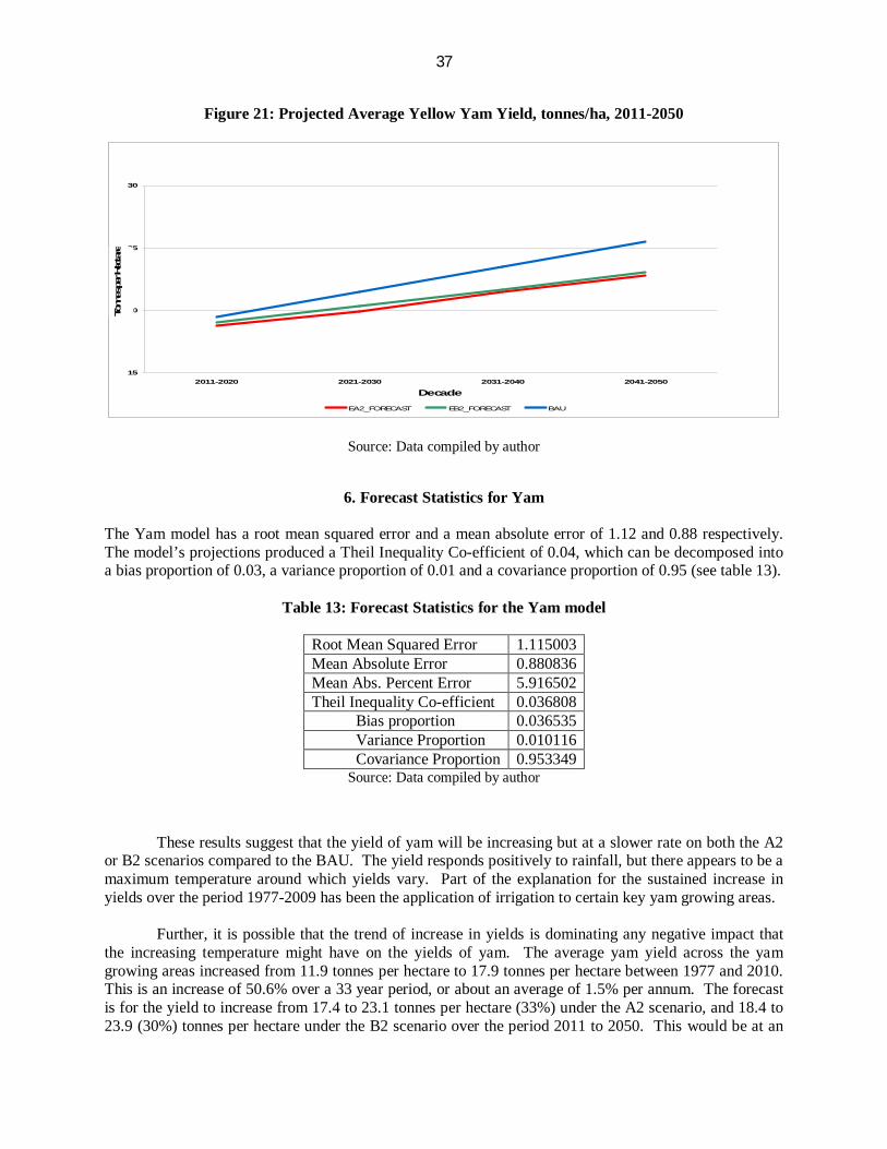
37

Figure 21: Projected Average Yellow Yam Yield, tonnes/ha, 2011-2050

15

20

25

30

2011-2020 2021-2030 2031-2040 2041-2050

Decade

Tonn

es p

er H

ecta

re

EA2_FORECAST EB2_FORECAST BAU


6. Forecast Statistics for Yam

The Yam model has a root mean squared error and a mean absolute error of 1.12 and 0.88 respectively. The model’s projections produced a Theil Inequality Co-efficient of 0.04, which can be decomposed into a bias proportion of 0.03, a variance proportion of 0.01 and a covariance proportion of 0.95 (see table 13).

Table 13: Forecast Statistics for the Yam model

Root Mean Squared Error 1.115003 Mean Absolute Error 0.880836 Mean Abs. Percent Error 5.916502 Theil Inequality Co-efficient 0.036808 Bias proportion 0.036535 Variance Proportion 0.010116 Covariance Proportion 0.953349


These results suggest that the yield of yam will be increasing but at a slower rate on both the A2 or B2 scenarios compared to the BAU. The yield responds positively to rainfall, but there appears to be a maximum temperature around which yields vary. Part of the explanation for the sustained increase in yields over the period 1977-2009 has been the application of irrigation to certain key yam growing areas.

Further, it is possible that the trend of increase in yields is dominating any negative impact that

the increasing temperature might have on the yields of yam. The average yam yield across the yam growing areas increased from 11.9 tonnes per hectare to 17.9 tonnes per hectare between 1977 and 2010. This is an increase of 50.6% over a 33 year period, or about an average of 1.5% per annum. The forecast is for the yield to increase from 17.4 to 23.1 tonnes per hectare (33%) under the A2 scenario, and 18.4 to 23.9 (30%) tonnes per hectare under the B2 scenario over the period 2011 to 2050. This would be at an

38

average annual rate of growth of less than 1%, somewhat slower than the annual average of 1.5% for the last 3 decades.

7. Modelling the yield of Escallion Using panel data for 6 parishes of Jamaica, a Fixed Effects Ordinary Least Squares Regression (Dummy-OLS) Model of the following functional form was estimated for escallion.

ititititititit

itit trendDttprpr

cpy 22 maxmax

where, ity - represents the yield of escallion per hectare. itc - represents the average cost of production per tonne in Jamaican dollars (J$), in a given

year itp - represents the average sale price in Jamaican dollars per tonne of escallion, in a given

year. pr - represents annual precipitation in millimetres.

ittmax - represents the average maximum monthly temperature, in a given year, in degrees Celsius

itD is a vector of dummy variables, which captures structural breaks in the time series36. ittrend captures the trend in yield per hectare.

The panel unit root tests (table 14) suggest that the yield of escallion, the ratio of price to production cost, temperature and annual rainfall are I(0).

Table 14: Unit Root Test

Variables Im-Pesara and Shin ADF-Fisher Levin, Lin and Chu t Escallion Yield 0.0041*** 0.0047*** 0.0127** Price/Production Cost 0.0000*** 0.0000*** 0.0001*** Temperature 0.0000*** 0.0000*** 0.0001*** Annual Rain 0.0000*** 0.0000*** 0.0001*** *** -Significant at the 1% level ** -Significant at the 5% level * -Significant at the 10%


The Fixed Effects Ordinary Least Squares Regression (Dummy-OLS) Model was estimated for

escallion. The model is limited by autocorrelation, and while the coefficients are unbiased, they are not the Best Linear Unbiased Estimator (BLUE). The model suggests that there is a positive relationship between escallion yield and the ratio of price to production cost37. A unit increase (decrease) in the ratio

36In 1992, the Ministry of Agriculture changed the way the units in which the data was recorded from output per acre to output per hectare. After adjusting the series for consistency, a break was still evident in the time series.

37 The ratio of price to production cost is held constant over the forecast period by using the arithmetic mean of the last 10 years of actual data

39

will lead to a 1.66 unit increase (decrease) in the yield of escallion per hectare. Since escallion is planted all year round total annual precipitation was used in the model. The model suggests that there is optimal maximum of rainfall for the crop per year of 2112.8 mm or, on average, 176.1 mm per month. By way of contrast, temperature has a minimum optimal of 29.5°Celsius per month. There is also a significant positive trend in yield per hectare, which, like yellow yam, suggests that over the period 1977 to 2009 production became more efficient (table 15).

Table 15: Factors determining the Yield of Escallion per year in tonnes per hectare

Escallion Model Regressors Coefficient P_values

Constant 952.2971 0.0114 **

Price/Production Cost 1.656697 0.0000***

Rainfall 0.005451 0.0248 **

Rainfall Square -1.29E-06 0.0399 **

Maximum Temp. -6.48E+01 0.0114 **

Maximum Temp. Squared 1.099493 0.0113 **

DUMMY 1.602883 0.0000***

DUMMYELIZ98 3.896615 0.0000***

DUMMYANN00 5.144469 0.0000***

DUMMYMAN 2.129756 0.0001***

DUMMYMAN2 8.677105 0.0000***

DUMMYELIZ -2.198558 0.0000***

@TREND 0.106679 0.0000***

F-statistic 304.3737 0.0000***

R-squared 0.966382

Adjusted R-squared 0.963208

Durbin-Watson stat 1.251581

Jarque-Bera 0.614686

Root MSE 0.976200 N 198

*** -Significant at the 1% level ** -Significant at the 5% level * -Significant at the 10%

Optimal Precipitation and Temperature Annual Rainfall 2112.8 Maximum Maximum Temperature 29.5 Minimum


8. Forecasts

Figure 22 shows the forecasts of the yield of escallion projected on the BAU, A2 and B2 scenarios. The model forecasts yields increase by all three scenarios but slower on the A2 and B2 scenarios than on the BAU.

40

Figure 22: Projected Average Escallion Yield (tonnes per hectare), 2011-2050

10.0

11.0

12.0

13.0

14.0

15.0

16.0

17.0

18.0

19.0

20.0

2011-2020 2021-2030 2031-2040 2041-2050Decade

Yiel

d pe

r hec

tare

EA2 EB2 BAU Source: Data compiled by author

9. Forecast Statistics for Escallion

The escallion model has a root mean squared error and a mean absolute error of 0.98 and 0.77 respectively. The model’s projections produced a Theil Inequality Co-efficient of 0.06, which can be decomposed into a bias proportion of 0.01, a variance proportion of 0.16 and a covariance proportion of 0.83 (see table 16).

Table 16: Forecast Statistics for the Escallion model Root Mean Squared Error 0.976521 Mean Absolute Error 0.770981 Mean Abs. Percent Error 14.72119 Theil Inequality Co-efficient 0.060676 Bias proportion 0.012690 Variance Proportion 0.161721 Covariance Proportion 0.825589


The difference between the yields for the A2 and B2 scenarios is very small. As with the forecasts of yam yields, the model’s forecasts suggest that yields will continue to increase up to 2050 in spite of changes in the temperature and precipitation conditions.

C. OTHER IMPACTS ON THE WIDER AGRICULTURAL SECTOR The approach to estimating the potential impact of climate change on agriculture in Jamaica adopted by this study was to focus on the dominant export crop and two of the most important domestic crops. Because of their relative weight in the GDP of agriculture, the intention was to extrapolate the potential impact on these crops to the sector as a whole. As shown above, the econometric results are ambiguous for the selected crops. In addition, whereas the econometric analysis focused exclusively on temperature and precipitation, there are other aspects of the climate that are changing which are likely to impact on agricultural activities. These are:

41

sea level rise, which will affect the salinity of the underground water sources and increase the risk of extreme wave actions;

Rising sea surface temperatures, that will increase the risk of coral bleaching with attendant negative impacts on reef life;

Flooding, alternating with periods of severe drought, as the precipitation pattern changes. Flooding and drought destroy crops. In addition, flooding increases the rate of soil erosion on the steep slopes cultivated by the small farming community, and drought increases the frequency of fires in all cultivations;

Increase in the rate of evaporation of soil moisture; Decrease in stream-flows. The Water Sector Adaptation Strategy developed by ESL in January

2009 forecasted the decline in flows for three major rivers in Jamaica – the Great River, the Hope River, and the Rio Grande River;

Higher temperatures will increase the breeding rate of pests and carriers of bacteria and viruses that are harmful to plants and animals.

While the scientific evidence for the link between climate change and the frequency of hurricanes

is mixed, there is a growing consensus that the intensity of hurricanes will increase. The Agriculture Disaster Risk Management Plan (ADRMP) noted that since the devastation caused by Hurricane Gilbert in 1988, there is evidence of enhanced resilience arising from greater awareness and preparedness especially at the community level. An indication of this is the practice adopted by fishermen of storing their boats and gear away from the beaches.

1. Sea level rise

The ESL 2009 study noted that the sea level is forecasted to rise by “0.18m to 0.59 m, possibly as high as 1.4m by 2090”, and as a result, there was a high risk of saltwater intrusion. There is already evidence of such intrusion as follows: “Saltwater intrusion has also degraded water quality along sections of the south coast in the St. Catherine and Clarendon Plains near the Black River and Alligator Pond and along the northern coast near Montego Bay.”38.

Also noted was the following:

“Many production water wells in the south are no longer pumped and many sugarcane fields have been abandoned. In the Rio Minho and Rio Cobre areas (central-southern part; 1 in figure 23) the increase in salinity is being observed at distance more than 10 km from the coast. However, one should point out that the saline intrusion along the south coast occurred prior to the 1961 period when the control of licensing was introduced onto the island. Since then the moratorium on new abstraction has reduced.”39

“Given the coastal location of many of Jamaica’s wells, for agriculture, public water supply and

industrial use, such increases in sea level increase the potential risk of saline intrusion into the coastal aquifers and thus the vulnerability of these wells in terms of negative water quality impacts.”40

38 ESL, 2009, p.73 39 Ibid, p.75 40 Ibid p.103

42

Figure 23: Contaminated Aquifers

Source: ESL, figure 3.7, p.75

2. Flooding “A 100 year review (1887-1987) of destructive events from natural hazards in Jamaica reveals one disastrous flood event every four years (WMORAIV Hurricane Committee, 1987)”41 At this rate, Jamaica can expect 10 more ‘disastrous floods’ between now and 2050. The flood of 2001 was classified by the ADRM as a major flood and the damage it caused was estimated to cost J$541 million42, or 2% of the agricultural GDP in that year. In the following year, 2002, heavy rains in the last week of May and the first week of June caused an estimated J$781 million, or 3% of agricultural GDP of in that year43.

3. Drought Because more than 90% of Jamaica’s agriculture is rain-fed, the sector is particularly vulnerable to drought in the bi-modal pattern of rainfall that obtains. According to the ADRM, the second most frequent hydro-meteorological hazard is drought. The drought of “December 1996 to 1998” caused $331.7 million dollars of damage or 1.4% of agricultural GDP in 1998.

4. Hurricanes According to the ADRM, “Since the 1850s when meteorological records became available for the Caribbean some 43 major storms have affected Jamaica of which over 16 percent were devastating category 3 and stronger --- ”and “Of the Category 3 and stronger storms impacting Jamaica since 1851, 57 percent occurred in the last decade (since 2000)”44.

41 Ibid, p.18 42 Balfour Spence, “Agriculture Disaster Risk Management Plan – Jamaica”, May 2009 43 See IDB-ECLAC, 2007, p.17, Table 4.2 44 ADRM, p.4,5

43

Table 17 presents some estimates of hurricane damage to the agriculture sector in recent years. Note that these estimates do not include damage to forests and fisheries, and tend to be conservative with regard to crop and livestock losses.

Table 17: Estimates of Hurricane Damage to Agriculture

Hurricane, Tropical Storm J$ billion % of Agriculture GDP 1988 Gilbert 8.8 2004 Ivan 8.55 27.6 2005 Emily, Dennis, Wilma 0.99 2.7 2007 Dean 3.76 9.1 2008 Gustav 1.63 3.3

Source: World Bank, “Toward a Strategy for managing agricultural weather risks”, June 2009, McGlashan and others, 2008

VI. ADAPTATION Adaptation to climate change in the agricultural sector is properly situated within adaptation strategies for the economy as a whole, and must take account of adaptation in other critical sectors. With regard to the national economy, mainstreaming climate change in national plans and policies is fundamental to coordinating the various sectoral initiatives. In terms of agriculture’s linkages with relevant sectors, the most immediate is with the water sector because of the critical dependence on water and the increasing importance of water for irrigating heat-stressed plants and preventing dehydration of animals.

“According to a report in 2005, although Jamaica signed the UNFCCC 13 years ago, it has not

achieved as much as could have been reasonably expected within the given time frame. The main reason for this may be the lack of sustained focus on climate change activities, perhaps due in part to the absence of the Climate Change Committee to guide and focus the country’s programmes. Other reasons could be the relatively low levels of public awareness with respect to the implications of climate change for national development, along with the absence of full political buy-in, in light of other pressuring social issues which are often the main focus of government actions.”45 Indeed, policy-makers have for decades been caught up in addressing the economic crisis, and consequently, not sufficiently engaged in resolving long term issues such as the actual and potential impact of climate change.

Jamaican agriculture must adapt to projected increases in temperature, shifts in rainfall patterns,

and extreme events such as hurricanes. While very little agriculture takes place on the island’s coasts which are vulnerable to sea level rise, the beaches that are used by fisherfolk as landing sites are threatened by the erosion it brings, and are vulnerable to extreme wave action. As such, communities of fisherfolk have been moving their boats and fishing equipment to higher ground to protect them from anticipated extreme wave action from hurricanes. This practice can evolve into an adaptation to permanent sea level rise that inundates some of the existing beaches. Crops cultivated inland, however, are at risk from the salination of underground aquifers.

A. INSURANCE Managing agricultural production in the context of climate variability is consistent with the development of strategies for adapting to climate change. One that was used in the early 20th century in Jamaica was 45 ECLAC 2010, p.75

44

crop insurance. More recently, a new form of insurance based on an index of probable weather outcomes has been advanced. “Weather indexed risk management products represent a newly developed alternative to the traditional crop insurance programs for smallholder farmers in the emerging markets. These products are based on local weather indices, ideally highly correlated to local yields. Indemnifications are triggered by pre-specified patterns of the index, not by actual yields. This reliance on factors beyond the control of farmers reduces the occurrence of moral hazard and adverse selection. It also eliminates the need for field visits, which speeds up claim settlement and significantly reduces costs. Because the insurance is based on a reliable and independently verifiable index, it can be reinsured, allowing insurance companies to transfer part of their risk efficiently to international markets.”46

Like traditional insurance, this approach to managing risk tends to favour increased productivity

in so far as it reduces the risk-aversion of the farmer to the adoption of new technologies and new crops. In addition to insurance, the principal adaptation strategies to climate change specific to agricultural crop and livestock production are:

Research into more heat-resistant plants. This is a natural area of collaboration between the

academic and farming communities. Jamaica has a good record of scientific research into the development, adoption and adaptation of plant and animal varieties to the local environment. The Sugar Industry Research Institute (SIRI) has a proud record of research into new varieties and cultivation practices for sugar cane. The work of T. P. Lecky in developing the Jamaica Hope breed of cattle is internationally recognized. In recent years, the University of the West Indies has been conducting research to develop food and medicinal products from Jamaican plants. In this regard, researchers need to engage the traditional knowledge of the farming communities47. It is this knowledge which has accumulated as folklore that has helped to sustain these communities for almost two centuries. There is a need for resources over and above the capabilities of the government to strengthen the research tradition. The scientific community will have to tap into available international funding for local research. In addition to primary research, the local academic community can facilitate the transfer of international knowledge of climate adaptable varieties to the local farming communities. Brazilian researchers estimated that it takes 15 years to develop a new variety of sugar cane.48 However, there are varieties that can be accessed from warmer areas than Jamaica for the ultimate replanting of the total crop. The estimate of the return to investment in research in sugar cane varieties in Barbados49 was put at 4 to 1.

Education of the farming community on the global, regional, and where possible, the national trends in climate change will enhance the abilities of the people to interpret changes in the local climate. This will enable them to build on their traditional knowledge of the local climate and become more conscious of the traditional adaptation strategies that have helped them to cope with the changes in the past. In addition, it will make them more receptive to national policies to adapt to climate change that impact both directly and indirectly on the sector. In addition to the schools for children in rural communities, public and private extension services will have to develop programmes to sensitize and teach farmers about climate change and the appropriate technologies to adapt to both climate variability and the longer run climate change. In this regard, the education programmes must be supported by information flows on weather, climate variability

46 Bryla and Syroka, 2007, p.3 47 Douglas W. Gamble and others, 2010 have conducted a study to “[integrate] local knowledge and perception of drought and its physical characteristics manifested in remotely sensed precipitation and vegetation data”, p.1 48New sugarcane varieties reduce costs and improve productivity 09/15/2010, http://english.unica.com.br/noticias/show.asp?nwsCode={9B7AAE53-8BC4-4576-8578-95D763B12E42} 49 De Boer and Bellamy, 1998

45

and climate change prepared by the Meteorological services in formats that are readily comprehensible by the farming community.

The majority of poor households are in rural communities with livelihoods based on agriculture, primarily subsistence activities supplemented with wage labour. The link between poverty and environmental despoliation for survival is well-known. Research into the environmental conditions in these communities will inescapably engage issues of poverty. Adaptation to climate change will offer opportunities for livelihoods for community members.

More and improved irrigation practices to better manage the provision of water to crops have long been recognized as a crucial service input for agriculture. Unlike export agriculture, domestic agriculture has traditionally been rain-fed, with farmers planting to “follow the rain”. Irrigation costs have been prohibitive, especially for farming areas in the hills that require water to be pumped from below. Here, the requirements of agriculture meet the requirements of the energy and water sectors, and the plans for the three have to complement each other and share a common alignment in public policy.

In a review of 192 irrigation projects funded by the World Bank, it was estimated that the average

internal rate of return on 67% of the projects deemed to be successful was 15%.50 RADA has designed a drip irrigation system for a 0.1 hectare plot based on a 1000 gallon tank on a reinforced tank base which costs approximately J$65,000.00. In addition, there is the cost of water which will vary according to its source. Rainwater harvesting is obviously the cheapest source. On average the tank can be filled twice per week, but in general, the rate of usage depends on the conditions such as the soil type, the daytime temperature, the type of crops, and others.

Jamaica as a whole and the agriculture sector in particular, needs better water management practices. The principal elements of this are:

o Management of the forests, so as to reduce the rate of deforestation, especially in the watershed areas. Forests in the hills also serve to hold the soil from being eroded as rainwater rushes down the steep slopes. Jamaica loses millions of hectares of topsoil annually to erosion from heavy rainfall in the hills. Furthermore, the soil eventually ends up in inshore and in the harbours producing negative consequences for coastal resources. In the case of the Kingston Harbour, the continual siltation of the harbour from run-off forces the Port Authority to conduct frequent dredging of the harbour at great financial and environmental costs. The wave of establishment of commercial coffee farms in the hills in the 1980s led to the denuding of the hill-sides and accelerated the erosion of the steep slopes of the parishes of St. Andrew and Portland. Similarly, in search of sticks for yam vines and fish pots, the mangroves on the coasts are exploited with less than due regard for their sustainability. Enforcement of environmental laws will be more effective, the more educated the farming communities are to the connection with their own livelihoods through climate impacts.

o Harvesting rainwater is essential both for household and farming needs as well as to minimize the destructive flows across the land. It has been proposed that the depressions and pits left from the mining of bauxite as mini-reservoirs be utilized and farmers be encouraged to acquire sealed tanks for storage at their houses and farms. Traditionally, roofs have been used as catchment surfaces to lead rainwater into tanks or barrels. Recent work at the UWI’s Mona Informatics has been mapping old waterways. This information will be useful for both avoiding cultivation and housing construction in flood prone areas, as well as for harvesting rainwater.

50 W. Jones, 1995, p.60

46

o Almost 175 years after Emancipation, there has still not been comprehensive land reform to give the propertyless ex-slaves, who constitute the majority of the population, access to land. After Emancipation, many ex-slaves illegally occupied Crown Lands and built their communities – houses, farms, roads, schools, churches, water supplies and so on – in defiance of the colonial government and without the assistance of what are today called international development agencies. The tradition of illegally occupying land has persisted to the present, with migrants from the rural areas establishing communities on marginal lands in the Kingston Metropolitan Area and other urban centres such as gully banks, swamps, and even river beds that have run dry.

One consequence of the settlement of steep slopes in rural hills and fragile lands in the urban centres is that often these settlements impede water courses and lead to flooding from even light rains. It is imperative that the government enforce the proper zoning of lands for agriculture and housing with a view to managing water run-off without the kind of flooding that has increasingly cost the country in terms of the damage and destruction of private property and public infrastructure, and loss of life. With regard to agriculture, as mentioned above, floods carry off a lot of top soil annually to the sea. Not only housing and other sectors compete with agriculture for land, but poor land and water management ultimately account for the loss of potential agricultural production. As the traditional pattern of rainfall changes, agriculture has to deal with both the lack of water in the form of severe droughts, and too much water even when light rains fall. Long term solutions reside in improved land and water management.

o Warmer weather has been shown to speed up the reproductive cycle of mosquitoes and other disease vectors. For agriculture, this portends more pests, in addition to the other sources of pests. Improved management of pests and diseases will be mandatory. An appropriate balance will have to be found between chemical and other methods of control since the former is costly to the health of both humans and the soil.

Adjusting the planting cycle to changing rainfall patterns has occurred in the past. With the acceleration of climate change, it will be necessary to anticipate the changes and adapt more quickly. ECLAC 2010 reports on the oral testimony of a rural teacher:

“When I was growing up, the 8th of August used to be the day to plant maize, and there were other dates for other crops, but now the farmers are confused by the weather and we have lost the certainty of when to plant crops”51

Education on climate change will ease the “confusion” of these farmers so that they can recognize the changes more quickly and adjust the planting cycle accordingly. To do so, farmers must develop confidence in the services of the Meteorological Office, which must be able to present technical information in a form that farmers can readily comprehend and understand the implications for their farming activities. Adjusting planting cycles will adjust the corresponding marketing cycle and in turn impact on farming household incomes. At the same time, domestic food supply and/or the export supply will be impacted by the changes. The social impacts of climate change are also to be consideres.

The practice of protecting cultivation using trees and shrubs as natural windbreaks is well-known and must be encouraged. While there is no consensus on the frequency of hurricanes in the future, a lot of evidence suggests that hurricanes will tend to be more intense. Accordingly,

51 ECLAC, 2010, p. 74

47

agriculture must prepare for extreme wind events. Windbreaks formed by trees strategically planted:

o Help to control soil erosion; o Cooler daytime temperatures, and warmer night-time temperatures; o Increase yields; o Reduce stress on animals thereby facilitating weight gain and reducing mortality of

young animals; o Can provide additional income from wood products, fruits, and fuel wood; o Enhance the habitats of birds and other forms of wildlife.

The decision about the choice of trees to plant as windbreaks, and in what array, will be determined by the shape and topography of the land, the direction of wind flows, the farm activities to be protected, the wood products targeted, and the cost. Helmers and Brandle [2005] estimated that an optimally space windbreak in the Great Plains of the United States of America resulted in increased yields of 7.61% and 9.23% respectively for corn and soybeans. While the Great Plains are prone to cyclonic activity of tornadoes, the Caribbean is prone to the cyclonic activity of hurricanes. Windbreaks will lower the risk of damage to crops and animals in extreme wind events like hurricanes.

Commercial agriculture in Jamaica is linked to protected agriculture by way of the construction of green houses. These too have to be strategically located in protected areas with disaster preparedness plans that allow for quick disassembly to minimize wind damage.

A lot of scientific work has been done on managing the temperature in chicken houses. Even so, in the face of increasing temperatures, ways will have to be found to improve the ventilation of chicken houses. This will probably entail more electrical power for fans, and therefore more costs to the farmers.

There are proposals52 to re-design poultry houses using new materials and more efficient cooling fans powered by cheaper no-fossil fuels to protect the birds from high temperatures. In lieu of that, the stocking density of houses should be reduced to allow for more air flow around and between the birds, while at the same time decreasing the natural heat from their bodies. Suitable designs and scales for Jamaica in the 21st century will, however, have to be determined, and these will have to inform new construction as well as retrofitting of extant poultry housing. As such costs will vary as farmers try to minimize heat-induced mortality rates.

Indeed, the ventilation of all animal houses, such as barns for cows and horses, will have to be improved to minimize the risk of heat stress to animals. The complement to this will be ready access to clean water both for drinking and for washing down the animals and their facilities.

52 See for example Czarick and van Wicklen, 2009

48

Ultimately, food security is the principal policy objective for agriculture. The 4th IPCC report suggested that agriculture in the temperate zones may benefit from warmer climates, even as the productivity of agriculture in the more tropical areas will suffer. This could lead to yet another reason for the increased international demand for food surpluses of developed countries with the consequent upward movements of international prices of food. Jamaica and the Caribbean must plan for such probable tightening of international food markets by pursuing the locally specific and appropriate adaptation strategies to climate change. One form of adaptation is the development of and/or expansion of crops to meet the needs of domestic food supply. In the event that wheat prices become prohibitive, it will become necessary to develop and promote blends of wheat with flour from local root crops, such as cassava and sweet potato. It is to be noted that the potential for regional integration presents itself even more urgently, not only as an economic platform for engaging the global economy, but as a plank in the strategies for adapting to climate change. For with the land resources of the continental countries – Guyana, Suriname and Belize – and the markets of Haiti, Jamaica and Trinidad, many food crops can be produced at competitive prices for relatively secure markets, provided the various political and legal obstacles to the movement of labour, capital and other resources to bring idle lands into production are addressed.

In a wide ranging study of adaptation measures, Adger and others (2007) noted that: “The

literature [on adaptation in agriculture] mainly reports on adaptation benefits, expressed in terms of increases in yield or welfare, or decreases in the number of people at risk of hunger. Adaptation costs, meanwhile, were generally not considered in early studies.”53 They go on to give a reason: “A particular limitation of adaptation studies in the agricultural sector stems from the diversity of climate change impacts and adaptation options but also from the complexity of the adaptation process. Many studies make the unrealistic assumption of perfect adaptation by individual farmers. Even if agricultural regions

53 Adger and others, 2007, p.725

Egg Production

A manual prepared for egg producers under the auspices of the Caribbean Poultry Association addresses the impact of heat stress on chickens. One of the main effects is the loss of appetite which affects growth, and for layers, causes reduced egg sizes, lower production and poorer shell quality. “When panting fails to prevent the rise in body temperature the bird becomes listless, then comatose, and soon dies.”1 Birds reared from young at high temperatures tend to adapt, but they too react to temperature spikes. The manual advises farmers on measures they can use to adapt to higher temperatures. Some of these are:

Provide the birds with plenty cool water Increase ventilation of the houses Avoid activity that will increase the body temperatures of the birds Prepare and administer more concentrated feed Design houses to facilitate more natural cooling that are insulated

from external heat, and that are made of materials that are cool. Houses should be oriented to minimize solar heating.

49

can adapt fully through technologies and management practices, there are likely to be costs of adaptation in the process of adjusting to a new climate regime.”54

1. Sugar cane Assumptions

Costs – no adaptation o These are defined to be the decrease of yields as compared to the BAU, valued in 2008

US$, and inflated by the GDP multiplier for export crops55, 1.7, on both scenarios A2 and B2

Costs – of adaptation. The two adaptation strategies are replanting with heat resistant sugar cane varieties, and establishing and rehabilitating irrigation systems. The adaptation strategies seek to offset the losses due to higher temperatures and shifts in the precipitation pattern. Other strategies to increase the yield of sugar cane, and ultimately, to increase the quantity of sugar that can be recovered from a tonne of sugar cane are assumed to be relevant whether or not there is adaptation to climate change.

o Plant 5000 hectares each year of 2012-2017 or a total of 30,000 hectares with heat resistant varieties. Thereafter, replanting with the same or similar heat resistant varieties and maintenance costs are assumed to be the same as would have occurred without adaptation to higher temperatures. That is, the costs of adaptation to higher temperature will be incurred in the first 6 years;

o Cost of replanting a hectare is US$1000 in 2008 prices; o The IDB estimated US$7000/ha for establishment of irrigation system and US$6000 for

rehabilitation56; o 76% of the 25000 hectares (19,000) that are irrigated are in sugar cane. Assume that over

the next 6 years, these are rehabilitated, and irrigation systems are established on the other 11.000 hectares;

o The inflation rate for Jamaica was conservatively estimated at 9.8% per year, the average for 1962 to 2009, after excluding 13 years with rates greater than or equal to 20% and as high as 77.3% in 1992. If all years were included, the average inflation rate would be 15.5% for 1962-2009. For the United States of America for 1962-2010, the inflation rate averaged 4.2%. The average rate of inflation for the United States of America was assumed for the calculations, since the estimates are expressed in 2008 USA dollar values;

o Amortization of irrigation equipment over 30 years; o Maintenance of irrigation equipment assumed to cost 2% of purchase value per year.

Table 18 shows estimates of (a) the costs of no adaptation according to both A2 and B2 scenarios in columns [2] and [3]; (b) the cost of adaptation by way of replanting with heat resistant varieties and establishing and rehabilitating irrigation systems for sugar cane farms in column [4]; and (c) the net benefits of adaptation on both scenarios in columns [5] and [6]. Recall that benefits on each scenario are the avoided costs of no adaptation.

54 Ibid, p.726 55 Supplied in personal correspondence with the Planning Institute of Jamaica

56 - IDB National Irrigation Development Program, http://idbdocs.iadb.org/wsdocs/getdocument.aspx?docnum=416673

50

Table 18: Comparative Costs of No Adaptation vs Net Benefits of Adaptation, 2012-2050 – Sugar Cane, US$ millions

Discount rate, %

Cost of no adaptation,

Scenario A2

Cost of no adaptation, Scenario B2

Cost of adaptation

Benefitsa under Scenario A

minus costs of adaptation

Benefitsb under Scenario B


[1] [2] [3] [4] [5] [6] 1 646.58 376.89 352.99 293.59 23.90 2 512.51 297.54 328.06 184.46 -30.51 4 331.16 189.87 289.28 41.88 -99.41

a Benefit = avoided loss under Scenario A2 b Benefit = avoided loss under Scenario B2

Source: Author’s compilation

By way of summary, table 18 shows that net benefits for the adaptation strategies recommended for sugar cane are positive at the three selected discount rates for avoided costs under Scenario A2, with the highest net benefits occurring when the discount rate is 1%. The net benefit of adaptation for Scenario B2 is positive only for a 1% discount rate. However, while net benefits on Scenario B2 are negative for the discount rates 2% and 4% respectively, the losses are much smaller than the losses that would occur under a no adaptation strategy. Table 19 presents the same estimates as in table 18 but as a percentage of GDP in 2008.

Table 19: Comparative Costs of No Adaptation vs Net Benefits of Adaptation, 2012-2050 – Sugar Cane, as a percentage of GDP in 2008

Discount rate, %

Cost of no adaptation

Scenario A2


Scenario B2

Cost of adaptation





[1] [2] [3] [4] [5] [6] 1 4.7 2.7 2.5 2.1 0.2 2 3.7 2.1 2.4 1.3 -0.2 4 2.4 1.4 2.1 0.3 -0.7



2. Yam Assumptions


US$, and inflated by the GDP multiplier for domestic crops57, 1.9, on both scenarios A2 and B2.

Costs – of adaptation. The adaptation is establishing drip irrigation systems, based on 1000 gallon plastic storage tanks designed for 0.1 hectare farms. This adaptation seeks to offset the loss due to the shift in the precipitation pattern, and reinforces the recent trend to utilize irrigation services for yam farming.

57 Supplied in personal correspondence with the Planning Institute of Jamaica

51

o Establish drip irrigation on 200 hectares each year of 2012-2021 or a total of 2,000 hectares;

o RADA estimated approximately US$7438.77/ha for establishment of a drip irrigation system, using a 0.1 ha farm as a model;

o The inflation rate for Jamaica was conservatively estimated at 9.8% per year, the average for 1962 to 2009, after excluding 13 years with rates greater than or equal to 20% and as high as 77.3% in 1992. If all years were included, the average inflation rate would be 15.5% for 1962-2009. For the United States of America for 1962-2010, the inflation rate averaged 4.2%. The average rate of inflation for the United States of America was assumed for the calculations, since the estimates are expressed in 2008 USA dollar values;

o Amortization of irrigation equipment over 30 years; o Maintenance of irrigation equipment assumed to cost 2% of purchase value per year.

Similarly, table 20 shows estimates of (a) the costs of no adaptation according to both A2 and B2

scenarios in columns [2] and [3]; (b) the cost of adaptation by way of establishing drip irrigation systems for small farms in column [4]; and (c) the net benefits of adaptation on both scenarios in columns [5] and [6]. Recall that benefits on each scenario are the avoided costs of no adaptation.

Table 20: Comparative Costs of No Adaptation vs Net Benefits of Adaptation, 2012-2050 – Yam, US$ millions

Discount rate, %

Cost of no adaptation, US$

million Scenario A2


million Scenario B2

Cost of adaptation, US$ million

Benefitsa under Scenario A2

minus costs of adaptation, US$

million



million [1] [2] [3] [4] [5] [6] 1 379.64 319.12 20.92 358.72 298.20 2 305.40 254.87 19.60 285.80 235.27 4 205.07 168.49 17.42 187.65 151.07



The net benefits are positive and large for adaptation for both scenarios, with the highest benefits occurring at discount rate 1%, and the lowest at 4%. Table 21 presents the same estimates as in table 20 as a percentage of GDP in 2008.

52

Table 21: Comparative Costs of No Adaptation vs Net Benefits of Adaptation, 2012-2050 – Yam, as a percentage of GDP in 2008

Discount rate, %


Scenario A2


Scenario B2

Cost of adaptation





[1] [2] [3] [4] [5] [6] 1 2.7 2.3 0.2 2.6 2.2 2 2.2 1.8 0.1 2.1 1.7 4 1.5 1.2 0.1 1.4 1.1

a Benefit = avoided loss under Scenario A2: b Benefit = avoided loss under Scenario B2 Source: Author’s compilation

3. Escallion

Assumptions


US$, and inflated by the GDP multiplier for domestic crops58, 1.9, on both scenarios Costs – of adaptation. The farmers of St. Elizabeth produce upwards of 75% of the escallion

output in very dry conditions. They have developed a technique of covering the roots of the plants with dried grass (mulching) to contain the moisture. Nevertheless, the farmers in that part of the country have been clamouring for a long time for water supply systems to support both household consumption and irrigation. Small scale irrigation systems, such as those recommended below, are being implemented, and are credited with the rapid rise in yields.

This study supports the long-standing recommendation for irrigation services. The adaptation is the establishment of drip irrigation systems, based on 1000 gallon plastic storage tanks designed for 0.1 hectare farms. This adaptation strategy seeks to offset the loss due to the shift in the precipitation pattern, and reinforces the recent trend to utilize irrigation services for escallion farming to complement the traditional practice of mulching.

o Establish drip irrigation on 100 hectares each year of 2012-2021 or a total of 1,000 hectares;

o RADA estimated approximately US$7438.77/ha for establishment of a drip irrigation system, using a 0.1 ha farm as a model;

o The inflation rate for Jamaica was conservatively estimated at 9.8% per year, the average for 1962 to 2009, after excluding 13 years with rates greater than equal to 20% and as high as 77.3% in 1992. If all years were included, the average inflation rate would be 15.5% for 1962-2009. For the United States of America for the period 1962-2010, the inflation rate averaged 4.2%. The average rate of inflation for the United States of America was assumed for the calculations, since the estimates are expressed in 2008 United States of America dollar values;

o Amortization of irrigation equipment over 30 years; o Maintenance of irrigation equipment was assumed to cost 2% of purchase value per year.

Similarly, table 22 shows estimates of (a) the costs of no adaptation according to both A2 and B2

scenarios in columns [2] and [3]; (b) the cost of adaptation by way of establishing drip irrigation systems for small farms in column [4]; and (c) the net benefits of adaptation on both scenarios in columns [5] and [6]. Recall that benefits on each scenario are the avoided costs of no adaptation. 58 Supplied in personal correspondence with the Planning Institute of Jamaica.

53

Table 22: Comparative Cost of Adaptation vs No Adaptation – Escallion

Discount rate, %


million Scenario A2


million Scenario B2

Cost of adaptation, US$ million



million



million [1] [2] [3] [4] [5] [6] 1 190.98 169.82 11.27 179.72 158.55 2 154.10 136.00 10.60 143.50 125.39 4 104.24 90.48 9.52 94.72 80.97

a Benefit = avoided loss under Scenario A2; b Benefit = avoided loss under Scenario B2 Source: Author’s compilation

As with yam, the net benefits of adaptation are positive and large for the three selected discount

rates for both Scenarios A2, and B2, with the highest net benefits occurring at a discount rate of 1% and the lowest at 4%. Table 23 presents the same estimates as in table 22 but as a percentage of GDP in 2008.

Table 23: Comparative Costs of No Adaptation vs Net Benefits of Adaptation, 2012-2050 – Escallion, as a percentage of GDP in 2008

Discount rate, %


Scenario A2


Scenario B2

Cost of adaptation





[1] [2] [3] [4] [5] [6] 1 1.4 1.2 0.1 1.3 1.1 2 1.1 1.0 0.1 1.0 0.9 4 0.8 0.7 0.1 0.7 0.6



It may be recalled that sugar cane accounted for an average of 59% of export agriculture GDP for the years 1964-2005, and root crops accounted for an average of 45% of domestic agriculture GDP for the years 1970-2005. Yam is the most important root crop, and together with escallion, they account for at least 40% of domestic agriculture GDP. Table 24 combines the estimates.

Table 24: Comparative Costs of No Adaptation vs Net Benefits of Adaptation, 2012-2050 – Sugar cane, Yam, and Escallion, as a percentage of GDP in 2008

Discount rate, %


Scenario A2


Scenario B2

Cost of adaptation





[1] [2] [3] [4] [5] [6] 1 8.8 6.2 2.8 6.0 3.5 2 7.0 4.9 2.6 4.4 2.4 4 4.7 3.3 2.3 2.4 1.0

a Benefit = avoided loss under Scenario A2; b Benefit = avoided loss under Scenario B2 Source: Author’s compilation

54

Table 25 combines estimates for all crops using all discount rates from 2012 – 2050.

Table 25: Net Benefit = Avoided loss under A2 minus Cost of adaptation, US$ million, at discount rate

1% 2% 4%

Sugar cane 229.74 223.47 211.90

Yam 24.44 23.30 21.26

Escallion 14.92 14.24 13.03 2012-20

Total 190.39 185.92 177.61

Sugar cane 67.27 59.37 46.53

Yam 92.50 80.66 61.73

Escallion 43.70 38.08 29.10 2021-30

Total 203.47 178.11 137.36

Sugar cane 246.72 197.52 127.62

Yam 108.65 86.06 54.49

Escallion 56.07 44.44 28.18 2031-40

Total 411.44 328.03 210.28

Sugar cane 209.34 151.03 79.64

Yam 133.13 95.78 50.17

Escallion 65.03 46.73 24.42 2041-50

Total 407.50 293.54 154.23 Source: Author’s compilation

These estimates probably account for about a half of the agricultural sector. While the full impact on the agricultural sector would be much less than twice these estimates, they should be seen as conservative estimates of the impact of climate change on agriculture, and the net benefits from adaptation.

A second best approach to estimating the net benefits of investments in adaptation was to use rates of returns based on reported results in similar circumstances internationally. Specifically, the rate of return on investment in research was taken from Barbados and Brazil; the rate of return for investment in irrigation was taken from a review of successful irrigation projects funded by the World Bank; the rate of return on investment in terracing was taken from a study of watersheds in Jamaica; and the rate of return on investment in windbreaks was taken from a study of the impact of windbreaks on yields of soybeans and corn in the Great Plains of the United States of America. Table 26 summarizes the adaptation strategies and the rates of return that have been adopted.

55

Table 26: Return on Investment in Adaptation

Cost Benefit Return on investment

Climate variability

Insurance Private

increased productivity because of reduced risk aversion to investments, risky choices of crops

Climate Change

Education Public-private partnership more attention to adaptation measures

Warming

Research, including accessing extant heat-resistant varieties Public-private partnership Increased yield Benefit/cost ratio = 4

Ventilation of non-poultry Animal houses Private cost

Minimize heat induced and related mortality rates, especially for cattle and pigs

Poultry houses Private cost Reduce heat-induced mortality rates

Change in precipitation pattern

Irrigation per ha Private cost Increased yield Internal rate of return = 15%

Terracing

Private (public) cost for private (public) hill-side lands

manage erosion, protect top soil, reduce the potential and impact of flooding

Internal rate of return =12-22%

Water Management

Individual catchment Private cost

Increased yield, reduced mortality of plants and animals

Public catchment Public cost Increased yield, counter drought

Public drainage Public cost Flood management Hurricanes

Windbreaks Private cost Manage the impact of winds on crops

increase in yields of corn and soybeans = 7.6%-9.2% respectively, for an optimally spaced windbreak in the Great Plains of the USA


56

VII. CONCLUSIONS AND RECOMMENDATIONS

This study sought to model the probable impact of climate change on the agricultural sector in Jamaica in the event that either SRES scenarios A2 and B2, based on ECHAM forecasts, obtain in the 21st century, particularly up to 2050. In the future, this work will have to be revised as more and better quality data are generated and collated, and as modelling techniques improve. The study focused on modelling the impact of climate change on the major export crop, sugar cane, and the two most important domestic crops, yam and escallion. The forecasts of the models under the two scenarios, A2 and B2, were compared with the forecasts under a scenario, called BAU (business as usual), that was derived by extrapolating the 30-year historical trends of temperature and precipitation. For each crop, the study investigated the costs and benefit of investing in adaptation options to projected increases in temperature and changes in the pattern of precipitation. The essential results are summarized in table 27. Table 27: Net Benefit = Avoided loss under each Scenario minus Cost of adaptation, US$ million, at

discount rate

Scenario A2 - costs of adaptation

Scenario B2 - costs of adaptation

1% 2% 4% 1% 2% 4% 2012-20 -229.74 -223.47 -211.90 -245.16 -239.20 -228.06 2021-30 67.27 59.37 46.53 59.72 51.37 38.27 2031-40 246.72 197.52 127.62 100.28 79.19 49.84 2041-50 209.34 151.03 79.64 109.06 78.12 40.55

Sugar cane

Total 293.59 184.46 41.88 23.90 -30.51 -99.41 2012-20 24.44 23.30 21.26 14.78 13.98 12.55 2021-30 92.50 80.66 61.73 66.99 58.38 44.61 2031-40 108.65 86.06 54.49 99.07 78.48 49.70 2041-50 133.13 95.78 50.17 117.37 84.42 44.21

Yam

Total 358.72 285.80 187.65 298.20 235.27 151.07 2012-20 14.92 14.24 13.03 8.97 8.48 7.59 2021-30 43.70 38.08 29.10 36.81 32.08 24.52 2031-40 56.07 44.44 28.18 51.33 40.66 25.75

Escallion

2041-50 65.03 46.73 24.42 61.44 44.18 23.11 Source: Author’s compilation

The results are mixed, depending on the discount rate used to compute the present values of costs

and benefits over the period 2012 to 2050. For sugar cane, replanting and irrigation appear to generate net benefits at the three selected discount rates for Scenario A2, but only at a discount rate of 1% for Scenario B2. For yam and escallion, investment in irrigation will earn significant net benefits for both Scenarios A2 and B2 at the three selected rates of discount -1%, 2% and 4%. The estimates will be improved with better estimates for the benefits for adaptation. Without scientific estimates for the increased yields resulting from adaptation, this study has had to rely on interpreting benefits as the avoidance of costs of no adaptation on both Scenarios A2 and B2 respectively. Further, it is possible that if the recommended adaptation strategies are part of a package of strategies for improving efficiency and hence enhancing competitiveness, the yields of each crop can be raised sufficiently to warrant the investment in adaptation to climate change.

57

The study also recognizes that farmers have long been adapting by way of changing planting cycles to more closely follow the rain, and in the case of escallion, developing techniques of “dry farming” using dried grass as mulch to contain the moisture in the soil around the roots of the plants. The recommended adaptation strategies are proposed as complements to traditional adaptation measures, however called.

Finally, this study is a first attempt to analyse the impact of climate change on agriculture with a

view to generating data to inform public policy to manage the impact. Many more attempts will be justified in the future as the impact of climate change becomes more perceptible and measurable, and the data needed to model the impact become more available and accessible. This last, the development of a supply of relevant data, will be crucial to making the necessary advances on this preliminary attempt.

58

REFERENCES

Adejuwon, J. (2005). Assessing the suitability of the EPIC crop model for use in the study of impacts of climate variability and climate change in West Africa. Singapore Journal of Tropical Geography, 26(1), 44 – 60. Adger, W.N., S. Agrawala, M.M.Q. Mirza, C. Conde, K. O’Brien, J. Pulhin, R. Pulwarty, B. Smit and K. Takahashi, 2007: Assessment of adaptation practices, options, constraints and capacity. (2007). Climate Change 2007: Impacts, Adaptation and Vulnerability. Contribution of Working Group II to the Fourth Assessment Report of the Intergovernmental Panel on Climate Change, M.L. Parry, O.F. Canziani, J.P. Palutikof, P.J. van der Linden and C.E. Hanson, Eds., Cambridge University Press, Cambridge, UK, 717-743. http://www.ipcc.ch/pdf/assessment-report/ar4/wg2/ar4-wg2-chapter17.pdf. Anthoff D., Hepburn C. & Tol R. (2009) Equity weighting and the marginal damage cost of climate change. Ecological Economics, 68, 836-849. Bryla, Erin and Joanna Syroka. (2007). “Developing Index-Based Insurance for Agriculture in Developing Countries”, Sustainable Development Innovation Briefs, Issue 2, United Nations, March 2007, http://www.un.org/esa/sustdev/publications/innovationbriefs/no2.pdf. Bueno, Ramon, Herzfeld, Cornelia, Stanton, Elizabeth A., Ackerman, Frank (2008). “The Caribbean and Climate Change – the Costs of Inaction”, Tufts University, May 2008. Bynoe, M. (2010). The Methodological Approach to the Review of the Economics of Climate Change Study in the Caribbean. Caribbean Community Climate Change Centre, Bliss Parade, Belmopan, Belize. Caricom Fisheries Unit, National Marine Fisheries Atlas. (2000). Caricom Fishery Report, No. 4, Belize, (2000), http://www.moa.gov.jm/files/Jam_NMFA.pdf. Cline, W.R. (1996). The impact of global warming on agriculture: a Ricardian analysis: comment. The American Economic Review 86(5), 1309 – 1311. Cline, W. R., (2007). Global Warming and Agriculture: Impact estimates by country, Centre for Global Development, 2007. Cummings, Mark. (2002). "Cane Farmers angered by replanting loans process", Jamaica Observer, April 17, 2002, http://www.jamaicaobserver.com/news/24185_Cane-farmers-angered-by-replanting-loans-process. Czarick, Mick and Gary van Wicklen , “15 Cost Saving Ideas for Poultry Housing”, 2009-04-07, http://www.wattagnet.com/15_cost-saving_ideas_for_poultry_housing.html. Darwin, R. (1999). The impact of global warming on agriculture: a Ricardian analysis: comment .The American Economic Review, 89(4), 1049 – 1052. De Boer H.G. and S.R. Bellamy, “Sugar Cane Research in Barbados and its Costs and Benefits”. 1998 Barbados Agricultural Management Company, Groves, St. George, Barbados, Proceedings South Africa Sugar Technology Association 72.

59

http://www.sasta.co.za/wpcontent/uploads/Proceedings/1990s/1998_de%20Boer_Sugarcane%20research%20in%20Barbados.pdf.

Deressa, T.T. (2007). Measuring the economic impact of climate change on Ethiopian agriculture: Ricardian approach. The World Bank Development Research Group Sustainable Rural and Urban Development Team. Retrieved from http://econ.worldbank.org. Downes A. S. and C. Pemberton (2009). “Climate Change and the Agricultural Sector in the Caribbean”, prepared for an ECLAC Project on “The Economics of Climate Change in the Caribbean”, October 2009. ECLAC, (2003). Older Persons in Latin America and the Caribbean: Situation and Policies – Summary, LC/L.73, 29 October 2003, prepared for the Regional Intergovernmental Conference on Ageing: Towards a Regional Strategy for the Implementation in Latin America and the Caribbean of the Madrid International Plan of Action on Ageing, Santiago, Chile, 19-21 November 2003. ECLAC (2010). “Review of the Economics of Climate Change (RECC) in the Caribbean project: Phase I – Climate Change profiles in Select Caribbean Countries”, LC/CAR/L.250, 3 February 2010. ESL Management Solutions Ltd. (2009). “Development of a National Water Sector Adaptation Strategy to Address Climate Change in Jamaica”, prepared for Mainstreaming Adaptation to Climate Change Project, January 2009. FAO, 2008. “Climate Change and Adaptation and Mitigation in the Food and Agriculture Sector”, Technical Background document from the Expert Consultation held on 5 -o 7 March 2008, Rome. Feenstra Jan F, Ian Burton, Joel B. Smith, and Richard S. J. Tol (eds). (1998). “Handbook on Methods for Climate Change Impact Assessment and Adaptation Strategies”, UNEP, October 1998. Fischer G., Shah M., Velthuizen H. & Nachtergaele F. (2006) Agroecological zones assessment. International Institute for Applied Systems Analysis. Reprinted from Encyclopedia of Life Support Systems (EOLSS), EOLSS Publishers, Oxford, UK. Fischer G., Shah M., Velthuizen H. & Nachtergaele F. (1996). Global Agroecological assessment for the 21st century. International Institute for Applied Systems Analysis. Gamble, Douglas W., Campbell, Donovan, Allen, Theodore L., Barker, David, Curtis, Scott, McGregor, Duncan and Popke, Jeff (2010) “Climate Change, Drought, and Jamaican Agriculture: Local Knowledge and the Climate Record”, Annals of the Association of American Geographers, 5 August 2010. Galindo, Luis Miguel. 2009. “Methodological Suggestions for the Climate Change Study” ECLAC. Gay, C., F. Estrada, C. Conde, H. Eakin, and L. Villers (2006). “Potential Impacts of Climate Change on Agriculture: A Case Study of Coffee Production in Vera Cruz, Mexico”, Centro de Ciencias de la Atmósfera, UNAM, Springer, 2006. Hansen, James W., Walter Baethgen, Dan Osgood, Pietro Ceccato, Robinson Kinuthia Ngugi, “Innovations in Climate Risk Management: Protecting and Building Rural Livelihoods in a Variable and Changing Climate”, http://www.icrisat.org/Journal/SpecialProject/sp13.pdf.

60

Helmers, Glenn and James R. Brandle, “Optimal Windbreak Spacing in Great Plains Agriculture” 2005. Great Plains Research 15 (Fall 2005): 179-98. http://digitalcommons.unl.edu/cgi/viewcontent.cgi?article=1796&context=greatplainsresearch&sei-redir=1#search="cost+benefit+wind+breaks". IDB, Jamaica - National Irrigation Development Program: Loan Proposal, (JA-0106), http://idbdocs.iadb.org/wsdocs/getdocument.aspx?docnum=416673. Iglesias, A., Garrote, L., Quiroga, S., & Moneo, M. (2009). Impacts of climate change on agriculture in Europe. PESETA-Agriculture study. Luxembourg: Office for Official Publications of the European Communities EUR – Scientific and Technical Research series. EUR 24107 EN – Joint Research Centre – Institute for Prospective Technological Studies. Jain, S. (2007). An empirical economic assessment of impacts of climate change on agriculture in Zambia. The World Bank Development Research Group Sustainable Rural and Urban Development Team. Retrieved from http://econ.worldbank.org. Jennings, P. G., R. C. Miller, D. L. Ffrench and B. G. Duffus, “Revitalization of the Jamaican Dairy Sector: Biogas as an Option for Enhancing International Competitiveness”, http://www.jddb.gov.jm/files/Publications/Revitalization%20of%20the%20Jamaican%20Dairy%20Sector%20III%20draft%20221.pdf Kirton, C. and M. Witter (2006). “Liberalization of the Jamaican economy and the Impact of Import Surges on Dairy, Poultry and Onion Production”, prepared for FAO, May 31, 2006. Little, Derek W (2010). “Jamaica’s Sugar Industry Beyond 2010”, presentation to the Commission of Inquiry into the Sugar Industry, July 12, 2010. Lobell, D.B., Cahill, K.N., & Field, C.B. (2007). Historical effects of temperature and precipitation on California crop yields. Climatic Change, 81, 187–203. Lozer ,Kemmehi (2008). “Privatisation of the Jamaica Sugar Industry: An Opportunity to Blaze a New Trail”, Sugar Industry Authority, Jamaica, November, 2008. Mano, R., & Nhemachena, C. (2007). Assessment of the economic impacts of climate change on agriculture in Zimbabwe: A Ricardian approach. The World Bank Development Research Group Sustainable Rural and Urban Development Team. Retrieved from http://econ.worldbank.org. McGlashan Don,Mitchell, Sylvia, Pryce, Michael, Ryan, Josette, McKenzie, Claudette, Burke, Adrian, Stirling, Shaunakay, Strong, Yvette, and Smith, Marcia 2008. “Jamaica: Country Report on the State of Plant Genetic Resources for Food and Agriculture”, September 2008. McGregor, Duncan, David Barker, and Donovan Campbell, “Environmental Change and Caribbean Food Security: recent hazard impacts and domestic food production in Jamaica”, http://www.americas.sas.ac.uk/events/docs/Food_crisis_papers/McGregor_etal.pdf. Mendelson R. & Kurukulasuriya P. (2008) How Will Climate Change Shift Agro-Ecological Zones and Impact African Agriculture? World Bank Policy Research Working Paper 4717. Retrieved from http://econ.worldbank.org. Mendelsohn, R., & Nordhaus, W.D. (1999). The impact of global warming on agriculture: a

61

Ricardian analysis: reply. The American Economic Review, 89(4), 1053 – 1055. Mendelsohn, R., & Nordhaus, W.D. (1999). The impact of global warming on agriculture: a Ricardian analysis: reply. The American Economic Review, 89(4), 1046 – 1048. Mendelsohn, R., & Nordhaus, W.D. (1999). The impact of global warming on agriculture: a Ricardian analysis: reply. The American Economic Review, 86(5), 1312 – 1315. Mendelsohn, R., Nordhaus, W.D., & Shaw, D. (1994). The impact of global warming on agriculture: a Ricardian analysis. The American Economic Review, 84(4), 753 – 771. Ministry of Agriculture and Fisheries, 2009. “Jamaica: Towards a Strategy for Financial Weather Risk Management in Agriculture”, November 3, 2009. Nordhaus W. & Yang Z. (1996) A Regional Dynamic General-Equilibrium Model of Alternative Climate-Change Strategies. The American Economic Review, {JEL H41, Q4, Q2, Q20). Ortiz R. A. & Markandya A. (2009) Integrated impact assessment models of climate change with an emphasis on damage functions. BC3 Working Paper Series, October 2009. Parry M. L. and T. R. Carter 1988. “The Assessment of Effects of Climatic Variation: Aims, Methods and Summary of Results”, in M. L. Parry, T. R. Carter and N. T. Konijn (eds) The Impact of Climatic Variations on Agriculture, Volume 1: Assessments in Cool Temperate and Cold Regions, Kluwer, Dordrecht, The Netherlands, p.11-96. PIOJ, “Vision 2030 – Final Draft Agriculture Sector Plan”, September 2009. Quam, Vernon C., John Gardener, James R. Brandle and Teresa K. Boes, “Windbreaks in Sustainable Agricultural Systems”, http://www.unl.edu/nac/morepublications/ec1772.pdf Quiggin, J., and Horowitz, J.K. (1999). The impact of global warming on agriculture: a Ricardian analysis: comment. The American Economic Review, 89(4), 1044 – 1045. Reinsborough, M.J. (2003). A Ricardian model of climate change in Canada. Canadian Journal of Economics, 36(1), 21 – 40. Report of the Sugar Industry Enquiry Commission, September 2010. Rivero Vega, Roger E (2008). “Workbook of Climate Change Impact in Agriculture: Basic Knowledge, Methodologies and Tools”, Camaguey Meteorological Centre, 2008. Rosenzweig Cynthia and Martin L. Parry. “Potential Impact of Climate Change on World Food Supply”, Nature vol. 367, 13 January 1994. http://pubs.giss.nasa.gov/docs/1994/1994_Rosenzweig_Parry.pdf. Seo N., Mendelson R., Dinar A., Kurukulasuriya P. & Hassan R. (2008) Long term adaptation: selecting farm types across agro-ecological zones in Africa. World Bank Policy Research Working Paper 4602. Retrieved from http://econ.worldbank.org. Sheng T.C (1989). “Soil Conservation for small farmers in the humid tropics”, FAO Soil Bulletin 60, 1989.

62

Simpson, M.C., Scott, D., New, M., Sim, R., Smith, D., Harrison, M., Eakin, C.M., Warrick, R., Strong, A.E., Kouwenhoven, P., Harrison, S., Wilson, M., Nelson, G.C., Donner, S., Kay, R., Geldhill, D.K., Liu, G., Morgan, J.A., Kleypas, J.A., Mumby, P.J., Christensen, T.R.L., Baskett, M.L., Skirving, W.J., Elrick, C., Taylor, M., Bell, J., Rutty, M., Burnett, J.B., Overmas,M., Robertson, R. and Stager, H. (2009). “An Overview of Modelling Climate Change Impacts in the Caribbean Region with contribution from the Pacific Islands”, United Nations Development Programme (UNDP), Barbados, West Indies, 2009. Smith, David A. Y (2007). Jamaica Country Report: Final Phase II for Component 1 Risk Information through National Pilot Studies”, prepared for IADB-ECLAC Project Information and Indicators Program for Disaster Risk Management, February 2007. Spence, Balfour (2009). “Agricultural Disaster Risk Management Plan – Jamaica”, May 2009. Stratus Consulting Inc, “Compendium on methods and tools to evaluate impacts of, and vulnerability and adaptation to, Climate Change”, prepared for UNFCCC, January 2005. Williams, Norman (2008). “Caribbean Poultry Association: Table Egg Production Manual”, 2008. Williams, Norman “Caribbean Poultry Association, Table Egg Production Manual”, 2008 William Jones, “The World Bank and Irrigation: A World Bank Operations Evaluation Study”, 1995, http://www-wds.worldbank.org/external/default/WDSContentServer/WDSP/IB/1999/09/11/000178830_9810191154281/Rendered/PDF/multi_page.pdf Witter M (2006). “Economic Implications of the transformation of the Jamaican sugar industry into a sugar cane based industry”, prepared for the Planning Institute of Jamaica, March 2006. Witter, M (2006). “Fiscal Expenditure on Services for Children in Jamaica, 2003/4 -2005/6”, prepared for UNICEF and the PIOJ, December 2006. World Bank, “Towards a Strategy for Managing Agricultural Weather Risks”, June 2009, http://www.moa.gov.jm/files/Agri_Weather_Risks/Carlos_Jamaica_AgInsuranceStrategy_June%2018%202009v2.pdf Wright, Paulette A. E (1999). “Influence of Temperature and Rainfall on Sugar Yields at Frome”, SIRI, 1999.

AN ASSESSMENT OF THE ECONOMIC IMPACT - document search

Documents

Transcript of AN ASSESSMENT OF THE ECONOMIC IMPACT - document search