Algorithmica (2009) 53: 425–453DOI 10.1007/s00453-007-9113-7

An Approximation Algorithm and DynamicProgramming for Reduction in HeterogeneousEnvironments

Pangfeng Liu · May-Chen Kuo · Da-Wei Wang

Received: 20 November 2006 / Accepted: 25 September 2007 / Published online: 30 October 2007© Springer Science+Business Media, LLC 2007

Abstract Network of workstation (NOW) is a cost-effective alternative to massivelyparallel supercomputers. As commercially available off-the-shelf processors becomecheaper and faster, it is now possible to build a cluster that provides high computingpower within a limited budget. However, a cluster may consist of different typesof processors and this heterogeneity complicates the design of efficient collectivecommunication protocols. For example, it is a very hard combinatorial problem tofind an optimal reduction schedule for such heterogeneous clusters. Nevertheless,we show that a simple technique called slowest-node-first (SNF) is very effectivein designing efficient reduction protocols for heterogeneous clusters. First, we showthat SNF is actually a 2-approximation algorithm, which means that an SNF schedulelength is always within twice of the optimal schedule length, no matter what kind ofcluster is given. In addition, we show that SNF does give the optimal reduction timewhen the cluster consists of two types of processors, when the ratio of communicationspeed between them is at least two. When the communication speed ratio is less thantwo, we develop a dynamic programming technique to find the optimal schedule. Ourdynamic programming utilizes the monotone property of the objective function, andcan significantly reduce the amount of computation time. Finally, combined with anapproximation algorithm for broadcast 2004, we propose an all-reduction algorithmwhich sends the reduction answer to all processors, with approximation ratio 3.5.

P. Liu · M.-C. KuoDepartment of Computer Science and Information Engineering, National Taiwan University, Taipei,Taiwan

P. Liu (�)Graduated Institute of Networking and Multimedia, National Taiwan University, Taipei, Taiwane-mail: pangfeng@csie.ntu.edu.tw

D.-W. WangInstitute of Information Science, Academia Sinica Nankang, Taipei, Taiwan

426 Algorithmica (2009) 53: 425–453

We conduct three groups of experiments. First, we show that SNF performs betterthan the built-in MPI_Reduce in a test cluster. Second, we observe a factor of 93times saving in computation time to find the optimal schedule, when compared witha naive dynamic programming implementation. Thirdly, we apply the theoretical re-sults to a branch-and-bound search and show that they can reduce the search time ofthe optimal reduction schedule by a factor of 500, when the cluster has three kinds ofprocessors.

Keywords Heterogeneous workstation cluster · Scheduling optimization ·Reduction protocol · Slowest-node-first heuristic · Dynamic programming ·Branch-and-bound search

1 Introduction

Network of workstation (NOW) is a cost-effective alternative to massively paral-lel supercomputers [1]. As commercially available off-the-shelf processors becomecheaper and faster, it is now possible to build a PC or workstation cluster that pro-vides high computing power within a limited budget. High performance parallelismis achieved by dividing the computation into manageable subtasks, and distribut-ing these subtasks to the processors within the cluster. These off-the-shelf high-performance processors provide a much higher performance to cost ratio so that ahigh performance cluster can be built inexpensively. In addition, the processors canbe conveniently connected by industry standard network components. For example,Gigabit technology provides up to 1 gigabit per second (Gbps) of bandwidth withinexpensive network adaptors and switches.

In parallel to the development of inexpensive and standardized hardware compo-nents for network of workstations, system software for programming on NOW arealso advancing rapidly. For example, the Message Passing Interface (MPI) libraryhas evolved into a standard for writing message-passing parallel code [13, 17, 27].MPI programmers use a standardized high-level programming interface to exchangeinformation among processes, instead of a native machine-specific communication li-brary. MPI programmers can write highly portable parallel codes and run them on anyparallel machine (including network of workstation) that has MPI implementation [9,12, 36].

Most of the literature on cluster computing emphasizes on homogeneous clust-ers—clusters consisting of the same type of processors. However, we argue that het-erogeneity is one of the key issues that must be addressed in improving performanceof NOW. First it is always the case that one wishes to connect as many processorsas possible into a cluster to increase parallelism and reduce execution time. Despitethe increased computing power, the scheduling management of such a heterogeneousnetwork of workstation (HNOW) becomes complicated since these processors willhave different communication performance from one another. Second, since most ofthe processors that are used to build a cluster are commercially off-the-shelf products,they will very likely be outdated by faster successors before they become unusable.Very often a cluster will consist of “leftovers” from the previous installation, and

Algorithmica (2009) 53: 425–453 427

“new comers” that are recently purchased. The issue of heterogeneity is both scien-tific and economic.

Any workstation cluster, be it homogeneous or heterogeneous, requires efficientcollective communications [2, 28, 29]. For example, a barrier synchronization is of-ten placed between two successive phases of parallel computation to ensure that allprocessors finish the first phase before any processor goes to the second. In addition,a scatter operation distributes input data from the source to all the other processors forparallel processing, then a global reduction operation combines the partial solutionsobtained from individual processors into the final answer. The efficiency of thesecollective communications will affect the overall parallel performance, sometimesdramatically.

The focus of this paper is to optimize the reduction operation. A 5-year-profiling inproduction mode at the University of Stuttgart has shown that more than 40% of theexecution time of Message Passing Interface (MPI) routines is spent in the collectivecommunication routines MPI Allreduce and MPI Reduce [29]. As a result it is vital todevelop efficient algorithm to collect and combine the data in a cluster environment,especially in a heterogeneous environment.

It is very intuitive that one might want to use a heterogeneous broadcast algorithm[6, 7, 10, 22, 25, 26] and work in the reverse direction for reduction, since if all thedata flow in the opposite direction, a broadcast becomes a reduction. However, this isnot the case because in a reduction every processor must send and contribute its data,so every processor must send at least one message. On the other hand, a broadcast isfor a single processor to send the same messages to all the other processors. Althoughother processor could help relay this message, but this relay will not necessarily makethe broadcast faster. For example, if there is an extremely fast processor that wants tobroadcast a message to a lot of other extremely slow processors, the best schedule isfor the fast processor to send the messages one by one to all other slow processors,without any replaying. In contrast the reduction operation requires every processor tosend exactly one message.

There has been some work in the literature that focus on the optimization of collec-tion reduction [19, 23, 29, 30]. However, these works consider mostly homogeneousenvironments, and does not take the diversity of processor speed into consideration—mostly because these approaches rely on recursive processor halving techniques andlow level communication protocol improvements, and they may not perform well inheterogeneous clusters. Vadhiyar et al. [33] gave an experimental approach to tunethe collective communication, including reduction, via exhaustive search on hetero-geneous clusters.

Heterogeneity of a cluster complicates the design of efficient collective communi-cation protocols. When the processors send and receive messages at different speeds,it is difficult to synchronize them so that the message can arrive at the right processorat the right time for maximum communication throughput. On the other hand, in ahomogeneous NOW every processor requires the same amount of time to transmit amessage. For example it is straightforward to implement a reduction operation on P

processors as logP phases, and in each phase we reduce the number of processorsthat have received the combined results from other processors by half. In a hetero-geneous environment it is no longer clear how to complete the same task within the

428 Algorithmica (2009) 53: 425–453

minimum amount of time. As a result, the focus of this paper is to propose algorithmsthat perform reduction efficiently in irregular and loosely coupled clusters, instead ofregular network topology, because homogeneous and regular network topology likebutterfly, can perform vector reduction much more efficiently.

This paper treats the heterogeneity of a cluster mathematically, and derives prov-ably efficient algorithms for reduction operations. The goal is to find an optimal re-duction schedule that uses the least amount of time to complete the reduction. Thispaper shows that a simple heuristic called slowest-node-first (SNF) is very effectivein designing reduction protocols for heterogeneous cluster systems. Despite the factthat SNF heuristic does not guarantee the optimal reduction time we show that SNFis actually a 2-approximation algorithm. That means for any cluster, the total SNFschedule length is guaranteed to be within twice of the optimal schedule length. Thisis very important since we prove that the performance of SNF is within twice of theoptimum, no matter what kind of cluster we are given. In addition, we show that SNFdoes give an optimal reduction time when the cluster consists of two types of proces-sors and the communication speed ratio between them is at least two. When the ratiois less than 2, we develop a dynamic programming to find the optimal schedule. Ourdynamic programming utilizes the monotone property of the objective function, andcan significantly reduce the amount of computation time.

Here is a summary of the theoretical results from this paper.

• SNF does give an optimal reduction time when the communication time of anyprocessor is a multiple of the communication time of any other faster processor inthe cluster.

• SNF is not optimal, but is a 2-approximation algorithm.• SNF does give an optimal reduction time when the cluster consists of two types of

processors and the communication speed ratio between them is at least two.• A dynamic programming to find an optimal reduction for cluster with two types of

processors, in time O(f 2s log s) where s and f are the number of slow and fastprocessors.

• A all-reduction algorithm with an approximation ratio 3.5.

It is a very difficult to find an optimal reduction schedule for heterogeneous clus-ters. In practice we often resort to branch-and-bound search [2]. This paper showsthat we can reduce the number of search tree nodes we have to examine by the theo-retical results developed in the proof of SNF results. We want to emphasize that theexhaustive search techniques in this paper are guided by the theoretical foundation,and these techniques can be incorporated into the framework suggested by Vadhi-yar et. al [33] that actually measures the key communication parameters, to furtheroptimize the search efficiency.

We conduct experiments to show that these techniques can improve the searchefficiency by a factor of 500 when there are three types of processors. For the caseof two types of processors, we experiment our dynamic programming and show thatour technique can reduce the amount of computation time by a factor of 93.

The rest of the paper is organized as follows. Section 2 describes the communi-cation model in our treatment of reduction problem in HNOW. Section 3 describesthe concept of earliest possible schedule and Sect. 4 describes the slowest-node-first

Algorithmica (2009) 53: 425–453 429

heuristic for reduction in heterogeneous cluster. Section 5 states the theoretical re-sults, including a special dynamic programming for efficiently solving a cluster thathas two kinds of processors. Section 6 describes how the theoretical results help im-prove the efficiency in finding optimal schedule, and Sect. 7 concludes.

2 Communication Model

There have been two classes of models for collective communication in homogeneouscluster environments. The first group of models assume that all the processors arefully connected. As a result it takes the same amount of time for a processor to senda message to any other processor. For example, both Postal model [5] and LogPmodel [20] use a set of parameters to capture the communication costs. In additionPostal model and LogP model assume that the sender can engage in other activitiesafter a fixed startup cost, during which the sender injects the message into the networkand is ready for the next message. Optimal broadcast scheduling algorithm for thesehomogeneous models can be found in [5, 20]. The second group of models assumethat the processors are connected by an arbitrary network. It has been shown that evenwhen every edge has a unit communication cost (denoted as the Telephone model),finding an optimal broadcast schedule remains NP-hard [14]. Efficient algorithms andnetwork topologies for other similar problems related to broadcast, including multiplebroadcast, gossiping and reduction, can be found in [11, 15, 16, 18, 24, 31, 34, 35].

Communication models for heterogeneous environments have also been proposedin the literature. Bar-Noy et al. introduced a heterogeneous postal model [4] in whichthe communication costs among links are not uniform. In addition, the sender mayengage in another communication before the current one is finished, just like homo-geneous postal and LogP model. An approximation algorithm for multicast is given,with an approximation ratio logk where k is the number of destinations of the mul-ticast [4]. Banikazemi et al. [2] proposed a simple model in which the heterogeneityamong processors is characterized by the speed of sending processors. Based on thismodel, a 2-approximation algorithm for broadcast is given in [25]. The approxima-tion ratio for the same algorithm is later improved to 1.5, and the problem is shownto be NP-complete in [22]. We adopt the simple model from [2] for its simplicityand the high level abstraction of network topology. Other models for heterogeneousclusters can be found in [8, 21].

The communication model of a heterogeneous environment is defined as follows.The system consists of n processors {p1, . . . , pn}, each is capable of direct point-to-point communication to one another. A processor pi is characterized by its transmis-sion time t (pi), i.e. the time it takes for pi to send a message to any other processor.

In order to make the communication model realistic, we further assume that twocommunications cannot overlap, i.e. neither the sender nor the receiver of an ongo-ing communication can engage in any other communication at the same time. This isreferred to as 1-port model in the literature [2, 3, 22, 25, 32]. Although communica-tion hardware often allows some degree of overlapping, e.g., a receiver may receiveseveral messages at nearly the same time by using MPI non-blocking routines, thisdegree of communication parallelism may be limited because processors may only

430 Algorithmica (2009) 53: 425–453

have only limited resource for communication, and multiple communications usingthe same resource eventually have to be serialized. As a result, we focus on thoseclusters in which all processors have very limited resources, and different communi-cations have to be serialized.

Despite that we model every processor by a “communication time”, the compu-tation time can also be incorporated into the model as follows. For every processorp we define its t (p) as the sum of the computation time to generate the data, plusthe communication time to delivery the data. For example, let a processor p receivethe data from another processor q , combine its data with the data of q , then sendthe combined data to another processor r . The computation time to generate the datacorresponds to combining the data of p with the data of q , and the communicationtime to delivery the data corresponds to sending combined data to processor r .

We define the reduction problem for the communication model we just described.Suppose each processor in the system has a unit of information, and we would like tocombine all these informations into the final answer, how do we schedule the proces-sors so that the reduction takes the least amount of time? For example, each processormay have a number and we want to compute the total sum of these numbers by mes-sage passing. For a homogeneous system a simple tree algorithm can be used so thatduring each iteration half of the processors send their information to the other halfwhere the informations are combined. The algorithm takes logn rounds, where n isthe number of processors, to combine all the informations since the number of activeprocessors reduces by half per iteration. However, due to the differences in commu-nication speeds within a heterogeneous environment, this algorithm cannot guaranteeminimum reduction time.

We formally define the reduction as a scheduling problem. We assume that thereduction operator is both associative and commutative, such that all possible combi-nations are valid. This assumption is based on the fact that all 12 MPI reduction oper-ators, including maximum, minimum, sum, product, logical and, logical or, etc., areassociative and commutative. We observe that during the reduction process exactlyn−1 messages are sent by n−1 different processors—each processor except the finalreduction destination, sends out exactly one message. Based on this observation, wedefine a reduction schedule as a mapping function from a processor to the time that itstarts sending its message. Formally we define a function s so that for any processorp (except the reduction destination), p starts sending its message at time s(p), andcompletes sending its message at time s(p) + t (p). Let c(s,p) = s(p) + t (p) be thecompletion time of p under the scheduling function s. The interval [s(p), c(s,p)] isdefined as the transmission window of p under s.

To show that it is not beneficial for the reduction destination to send out any mes-sage, we define that a processor p can reach the reduction destination d if and onlyif there exists a series of transmission windows w1,w2, . . . ,wk , and the followingproperties are true.

1. The source of w1 is p.2. The destination of wk is d .3. The destination of wi is the source of wi+1, for 1 ≤ i < k.4. The starting time of wi+1 could not be earlier than the ending time of wi , for

1 ≤ i < k.

Algorithmica (2009) 53: 425–453 431

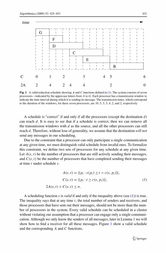
Fig. 1 A valid reduction schedule showing A and C functions defined in (1). The system consists of sevenprocessors—indicated by the uppercase letters from A to G. Each processor has a transmission window toindicate the time interval during which it is sending its message. The transmission times, which correspondto the duration of the windows, for these seven processors, are 10, 5, 5, 5, 4, 2, and 2, respectively

A schedule is “correct” if and only if all the processors (except the destination d)can reach d . It is easy to see that if a schedule is correct, then we can remove allthe transmission windows with d as the source, and all the other processors can stillreach d . Therefore, without lose of generality, we assume that the destination will notsend any messages in our scheduling.

Due to the constraint that a processor can only participate a single communicationat any given time, we must distinguish valid schedule from invalid ones. To formalizethis constraint, we define two sets of processors for any schedule at any given time.Let A(s, t) be the number of processors that are still actively sending their messages,and C(s, t) be the number of processors that have completed sending their messagesat time t under schedule s.

A(s, t) = |{pi : s(pi) ≤ t < c(s,pi)}|,C(s, t) = |{pi : t ≥ c(s,pi)}|, (1)

2A(s, t) + C(s, t) ≤ n.

A scheduling function s is valid if and only if the inequality above (see (1)) is true.The inequality says that at any time t , the total number of senders and receivers, andthose processors that have sent out their messages, should not be more than the num-ber of processors in the system. Every valid schedule can be scheduled in a clusterwithout violating our assumption that a processor can engage only a single communi-cation. Although we only know the senders of all messages, later in Lemma 1 we willshow how to find a receiver for all these messages. Figure 1 show a valid scheduleand the corresponding A and C functions.

432 Algorithmica (2009) 53: 425–453

3 Earliest-Possible Schedule

This section describe a technique called earliest possible scheduling that can “nor-malize” all the possible valid schedules. We use this canonical form to simplify thediscussion of finding an optimal schedule.

An earliest possible (EP) schedule is one in which all the communications areinitiated as earlier as possible. A new communication can be initiated as soon as thenumber of free processors reaches 2—one for the sender and one for the receiver.Let F(s, t) denote the number of processors that we are free to use to initiate a newcommunication at time t under schedule s. That is, F(s, t) = n − 2A′(s, t) − C(s, t),where A′(s, t) = |{pi |s(pi) < t < s(pi) + t (pi)}| is the number of processor thatare in the middle of sending and receiving messages. Note that A′(s, t) is differentfrom A(s, t). A′(s, t) does not include processors that will start sending and receivingmessage at time t but A(s, t) does. As a result all the first �n/2� processors will startsending messages at time 0, and the rest of the processors will start sending messagesas soon as the number of free processors reaches two, as illustrated by Fig. 2. Notethat after a message is received, only the receiver is considered “free” since it has theinformation from the sender, and should be kept active. The sender will no longer be“free” and will not participate in any further communication. The algorithm EP willassign non-decreasing start time to the processors in the order they appear in the inputprocessor sequence P . Since we do not need to schedule the reduction destination forsending, there are only n − 1 processors in the input processor sequence P .

By definition an earliest possible schedule s has the following properties.

1. n − 1 ≤ 2A(s, t) + C(s, t) ≤ n.2. For any processor p that s(p) > 0, there exist another processor q such that s(p) =

c(s, q).

Note that it is trivial to convert any valid schedule into an EP schedule withoutincreasing the total time—we just move the transmission window of each processor

Fig. 2 The pseudo code for theearliest possible schedulingalgorithm

Algorithm EP(P){

i = 1; time = 0; free = n;Active = empty set; Complete = empty set;while (i ≤ n-1) {

do while (free ≥ 2) {set the start time of the i-th processor in P to timeadd the i-th processor in P into Active;i = i + 1;free = free − 2;

}find the set of processors p that has the smallestcompletion time in Active;time = the completion time of p;move p from Active to Complete;free = free + the number of elements in p ;

}}

Algorithmica (2009) 53: 425–453 433

Fig. 3 The EP schedule converted from the schedule in Fig. 1. Note that when time is 2, both processors G

and F have completed sending their messages, and will no longer be “free” (C = 2). Meanwhile processorD is sending its message to another processor (2A′ = 2). The number of “free” processors is 7−2−2 = 3,which is more 2, the number of initiating another communication. Therefore we can initiate processor C

to start sending another message. Now we have 2A = 4 and the number of free processors is below 2

to the earliest possible time. As a result EP schedule servers as a canonical form inwhich we will limit our search of an optimal schedule. Since the EP algorithm cancompletely determine a schedule once the order of processors in the sequence P isfixed, we only have to consider up to (n− 1)! different schedules. Figure 3 shows theEP schedule that is converted from the schedule in Fig. 1.

3.1 Sender Dependency and Destination Assignment

Given an EP schedule, we need to specify the destinations for all messages in order toprogram a cluster to perform a reduction. We will show that under any EP schedule,it is always possible to do so without violating the constraint that a processor cannotparticipate more than one communication simultaneously.

Lemma 1 For any earliest possible schedule we can assign the destinations for allprocessors so that no two overlapping transmission windows have any sender or re-ceiver in common.

Proof First we would like to establish the dependency among the processors. Notethat in algorithm EP it requires two free processors to start a new transmission. Recallthat only the receiver of a communication remain “free” after the message passing,we need to wait for two communications to finish in order to have two new freeprocessors. As a result we define the predecessors of a sender processor to be the twosenders that must complete before the new transmission can start.1 This dependencyforms a binary tree among all sender processors.

1Note that when n is an odd number, one of the processor will have only one predecessor.

434 Algorithmica (2009) 53: 425–453

Fig. 4 Find the destinations for all senders in Fig. 3. Note that A is the destination processor

Now we can start filling in the destinations for all senders. First we assign the re-duction destination d as the destination of the sender that has the latest completiontime. Then for a sender/receiver pair s and r , we assign s and r to be the destinationsof the two predecessors of s. We assign destinations for transmission windows in atop-down manner within the binary dependency tree. Since both predecessors com-plete sending their messages before s starts, no overlapping transmission windowswill have processors in common. �

Figure 4 shows an example of how to find the destination for the schedule in Fig. 3.Note that the assignment is not unique since we can assign s and r to either of thetwo predecessors.

4 Slowest-Node-First Scheduling

We now introduce a simple scheduling heuristic called slowest-node-first (SNF) forthe reduction problem. SNF simply sorts the processors in P = (p1,p2, . . . , pn−1) innon-increasing transmission time order, i.e., t (pi) ≥ t (pj ) if i < j . SNF then givesthe sorted sequence P to algorithm EP for scheduling. In the next section we showthat this simple technique is very effective in obtaining a good reduction schedule.Figure 5 shows the slowest-node-first schedule with the same cluster as in Fig. 3.

The rationale of having the slowest processors to send messages first is as follows.At the beginning of the reduction process, we would like to overlap as many commu-nication windows as possible. Intuitively we let all the slow processors send first sothat they will overlap with each other, instead of having to wait for each other at theend of the reduction.

5 Theoretical Results

Before we describe the main results, we describe an exchange lemma that clarifiesour intuition that slow processors should send first, as we did in SNF scheduling.

Algorithmica (2009) 53: 425–453 435

Fig. 5 Slowest-node-firstscheduling result from the samecluster as in Figs. 1 and 3

Fig. 6 An illustration on thecontribution to the sum of C and2A before and after we switchthe transmission windows of p

and q

Lemma 2 Let s be a valid schedule and processor p starts right after processor q

ends, i.e. s(p) = c(s, q). If t (p) > t(q) then we can exchange p and q so that themodified schedule s′ in which s′(p) = s(q) and s′(q) = c(s′,p) is also valid.

Proof From Fig. 6 we observe that the contribution of p and q to the sum of C andA functions is always higher in s than in s′, therefore if s can satisfy Inequality 1, socan s′. �

From Lemma 2 it follows that in the search of an optimal reduction schedule wecan neglect those schedules that have a slower sender p with a faster predecessor q .There are two cases to consider. First if s(p) = c(s, q) then by Lemma 2 we canswitch p and q . On the other hand, if there is a gap between the transmission windowsof p and q , then we can delay the window of q until it touches p’s window. We cando so because there is no new transmission initiated between s(p) and c(s, q), sinceq is a predecessor of p. As a result we will consider only those schedules that all thesenders have predecessors of smaller or equal transmission time.

436 Algorithmica (2009) 53: 425–453

Corollary 1 There exists an optimal schedule such that the predecessors of everysenders have an equal or higher transmission time than the sender.

5.1 Approximation Ratio

We now consider a special class of clusters in which the transmission time of everyprocessor is a power of 2. Without lose of generality we assume that the fastestprocessor has a transmission time of 1. We call this kind of cluster a power 2 clusterand show that SNF generates optimal schedules for all power 2 clusters.

Theorem 1 The slowest-node-first method gives optimal schedules for all power 2clusters.

Proof We show that every schedule for a power 2 cluster can be converted into theSNF schedule without increasing the total reduction time. We reschedule all the slow-est processors as early as possible, until there is no faster processor ahead of them.Then we reschedule the second slowest processors the same way, and repeat thisrescheduling until the final schedule is the same as SNF.

When the transmission time of every processors is a power of 2, we claim thatthere is an optimal schedule s so that for every processor p its starting time s(p) isa multiple of its transmission time t (p). Since every processor has a predecessor thatends when it starts, we locate a “chain” of predecessors all the way back to time 0. Inaddition, every one of these predecessors has a transmission time of equal or largerpower of 2. Therefore the start time s(p), which is the sum of the transmission timeof these predecessors, is also a multiple of its transmission time.

Consider a processor p and the set F of faster processors that starts before p. Letq be the processor that completes last in F . If q finishes right when p starts, then byLemma 2 we can exchange p and q . If there is a gap between s(p) and s(q) + t (q),we claim that there will be no transmission windows located within this gap. If aprocessors starts or ends within this gap it must fall into this gap completely, sinceall processors must start and end at the multiple of its transmission time. If that is thecase q will not be the processor with the largest completion time in F . Since there isno transmission window in the gap, we can safely delay the transmission window ofq so that q ends when p starts. By Lemma 2 we can then exchange p and q and thetheorem follows. �

Theorem 2 The slowest-node-first schedule has a total reduction time no greaterthan twice of the time of an optimal schedule.

Proof Let s be an optimal schedule for a cluster H . Without lose of generality weassume that the fastest processor in H has a transmission time 1. We first convert H

into a power 2 cluster by increasing the transmission time of every processor p to2�log t (p)�. We call this new cluster H ′.

We argue that there exists a schedule s′ for H ′ in which every processor p startsat time no later than 2s(p). The claim follows from a simple induction that if everyprocessor p in H ′ waits for the two predecessors q and r defined by s, then it can

Algorithmica (2009) 53: 425–453 437

start at time no later than 2s(p), since both p and q starts no later than 2s(q) and2s(q), and their transmission time at most doubles in H ′.

Now we have constructed a new schedule s′ for H ′ that has a reduction time atmost twice of s. Since s′ is a schedule for a power 2 cluster, its reduction time is atleast the time of the optimal SNF schedule s∗ on H ′. Finally if we apply SNF onH and obtain schedule s′′, it will be as fast as the SNF schedule s∗ on H ′, since forevery processor both of its predecessors can start earlier and send messages faster. Asa result the reduction time of s′′ is no more than s∗, which in turn is no more thantwice of s. �

5.2 Approximation Ratio for All-reduction

There is a similar problem called all-reduction, in which the final reduction answershould be sent to all processors. It is easy to see that the all-reduction is at leastas expensive as a fastest broadcast from any source, or a fastest reduction into anydestination.

In a previous paper [25] we showed that starting from any processor as the source,we can perform a broadcast in no more than twice of the fastest broadcast time fromthat same source, with an technique called fastest-node-first [2]. The fastest-node-first technique is later shown to have an approximation ratio 1.5 when the broadcastsource is the fastest processor [22]. We have already shown that with slowest-node-first scheduling, we can perform reduction to any destination with time no more thantwice the optimal time to the same destination. Combining these two algorithms, wecan perform an all-reduction within 3.5 times of the optimal time. We first performa reduction into the fastest processor with SNF, which will complete in twice of theoptimal all-reduction time, then we do a broadcast from that fastest processor, whichtakes at most 1.5 times of the optimal all-reduction time.

Theorem 3 There exists a 3.5-approximation all-reduction algorithm. That is, thisalgorithm gives an all-reduction schedule and the length is within 3.5 times of theoptimal schedule, for all possible clusters.

5.3 Two Types of Processors

In this section we prove that SNF does give the optimal reduction time when thecluster consists of two types of processors, and the communication speed ratio be-tween them is at least two. We also find a counterexample which shows that if thecommunication speed ratio between them is less than two then SNF is not optimal.

Lemma 3 Let s be a valid schedule, p be a slow processor and q1, q2, q3 be fastprocessors. If s(p) is within the transmission window of q1, q1 stars right after q2,and q2 starts right after q3, then there exists a schedule s′ with following properties.

1. s′(p) = s(q3), i.e. process p starts sending message in s′ the time process q3 startssending message in s.

438 Algorithmica (2009) 53: 425–453

Fig. 7 Rearrange the communication windows of p and q1, q2, q3

2. s′(q3) = s(p), i.e. process q3 starts sending messages in s′ the time process p

starts sending message in s.3. Process q1 starts right after q2 and q1 ends in s′ at the same time as p ends in s.

Proof From Fig. 7 we observe the followings:

1. 2A(s, s(p)) + C(s, s(p)) = 6 because p is at least twice as slow as q1.2. s′(q2) < c(s′,p), i.e. p ends before q2 starts in s′.

From the observations above we conclude that at any time t the value of 2A + C

is always equal or higher in s than in s′, and the lemma follows. �

According to Lemma 2 we know that there exists an optimal schedule in whichno slow processor will start right after a fast processor. Therefore, we can assumefor every slow processor, its predecessors are slow processors as well. As a result thestarting time of every slow processor is a multiple of its transmission time, and wecan layer the slow processors according to their starting time as follows.

Definition 1 Layer one processors are the set of slow processors starting at time 0.Layer i +1 processors are the set of slow processors starting right after layer i proces-sors.

Theorem 4 SNF is optimal when there are only two types of processors and thecommunication speed ratio between them is at least two.

Proof Assume that there exists an optimal solution in which there exits a slow proces-sor that starts after a fast processor does. Let p be the earliest such slow processor,and q be the last fast processor starts before p starts. We show that it is always pos-sible to reschedule p so that it starts earlier than q without increasing the total time.

There are three cases to consider—processor p can start before, at, or after theprocessor q ends. For the second case we apply Lemma 2 and switch p and q . For

Algorithmica (2009) 53: 425–453 439

Fig. 8 A counterexample thatSNF always gives optimalreduction time in a clusterconsisting of two types ofprocessors

the third case, since q finishes last among all the fast processors starting before p,there will be no processor starting in the gap between q ends and p starts. As a resultwe can delay the transmission window of q so that q ends right when p starts, thenwe apply Lemma 2 to move p earlier.

We now consider the first case. Since every processor has a predecessor that endswhen it starts, we locate a “chain” of predecessors for q all the way back to time 0. Forprocessor q we need at least two levels of predecessors and both of them must be fastones, since the ratio of communication speed is at least two and the slow processorsmust start at a multiple of its transmission time. By Lemma 3 we find a new schedulein which p starts before q . We repeatedly reschedule the slow processors p earlieruntil no fast processor starts before it, and the theorem follows. �

Figure 8 shows a counterexample that SNF always gives optimal reduction time.This cluster has 4 slow processors with transmission time x, and 8 fast processorswith transmission time 1. The alternative schedule requires 2x + 1 time when 1.5 ≤x < 2, or 4 when 1 < x < 1.5. In contrast SNF requires x + 3 time for both cases,and has a longer reduction time for all x between 1 and 2. As a result the bound oftwo in Theorem 4 is tight.

5.3.1 Small Speed Ratio

From the counter-example in Fig. 8, we know that SNF cannot find optimal solu-tion for a cluster of only two types of processors with speed ratio no more than 2.However, in the following we show that we can still use dynamic programming tofind the optimal solution in this situation. In addition, we show that this dynamicprogramming can be significantly improved by a theoretical study.

To ease the explanation we suggest a binary tree representation for the reductionproblems. Figure 9 illustrates a reduction problem. Now if we traverse backwardin time, we obtain Fig. 10, which has the same total time as in Fig. 9. For each

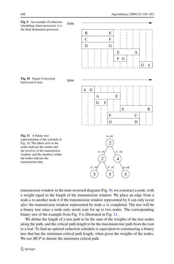
440 Algorithmica (2009) 53: 425–453

Fig. 9 An example of reductionscheduling where processor A isthe final destination processor

Fig. 10 Figure 9 traversedbackward in time

Fig. 11 A binary treerepresentation of the schedule inFig. 10. The labels next to thenodes indicate the sender andthe receiver of the transmissionwindow, and the numbers withinthe nodes indicate thetransmission time

transmission window in the time-reversed diagram (Fig. 9), we construct a node, witha weight equal to the length of the transmission window. We place an edge from anode a to another node b if the transmission window represented by b can only occurafter the transmission window represented by node a is completed. The tree will bea binary tree since a node only needs wait for up to two nodes. The correspondingbinary tree of the example from Fig. 9 is illustrated in Fig. 11.

We define the length of a tree path to be the sum of the weights of the tree nodesalong the path, and the critical path length to be the maximum tree path from the rootto a leaf. To find an optimal reduction schedule is equivalent to constructing a binarytree that has the minimum critical path length, when given the weights of the nodes.We use MCP to denote the minimum critical path.

Algorithmica (2009) 53: 425–453 441

5.3.2 Dynamic Programming

Before we describe the dynamic programming algorithm for finding the minimumcritical path, we make the following observation. From Observation 1 we immedi-ately conclude that there exists an optimal MCP tree in which all the fast nodes areon top of slow processors in the tree, that is, no slow processor has fast child.

Observation 1 An MCP tree exists in which every node has a cost no greater thanits children.

This observation follows from the fact that if an MCP tree does have a parentwith a cost larger than one of its children, we switch these two nodes and the overallMCP length will not increase. In fact this is a special case of Lemma 2. We can alsoconclude that an optimal MCP tree exists in which every path from the root to a leafhas non-decreasing weights on the nodes.

We describe a dynamic programming method for finding the optimal MCP treefor clusters with two classes of processors. From Theorem 4 we only need to focuson the cases where the speed ratio is less than 2. Let T (f, s) be the minimum criticalpath length for a cluster consisting of f fast processors, s slow processors, and adestination whose transmission time is irrelevant. The transmission time of fast andslower processors are tf and ts respectively. We define T (f, s) recursively as thefollowing (2). This recursion follows from Observation 1 that an optimal MCP treeexists with the root being the minimum cost in the tree - in our case a fast processor.

T (f, s) = tf + minfl+fr=f −1

sl+sr=s

(max(T (fl, sl), T (fr , sr ))), f > 0 (2)

= �log2(s + 1)�ts , when f = 0. (3)

The recursion above suggests a dynamic programming solution to the MCP prob-lem. The optimal solutions of MCP are kept in a two dimensional array, with thenumber of fast and slow processors as the indices. The algorithm makes these tableentries from lower to higher indices. The execution time, given f and s as the numberof processors, is bounded by O(f 2s2), since there are f s entries to compute, and thetime for computing each entry is bounded by O(f s) time.

5.3.3 Improvement from the Monotone of s Coordinate

The dynamic programming described in the previous section can be improved if weunderstand the structure of the T (f, s) function. We describe this structures and showhow it reduces the computation costs of T (f, s). It is not difficult to see that theT (f, s) function is monotonic with respect to s, that is, when we increase the numberof slow processors, the optimal MCP length will not decrease.

Lemma 4 T (f, s + 1) ≥ T (f, s) for all s ≥ 0.

Proof Consider an optimal MCP tree T with f fast and s + 1 slow processors. Sup-pose this tree has a shorter MCP than the tree with one less slow processor, that is,

442 Algorithmica (2009) 53: 425–453

T (f, s + 1) < T (f, s). From Observation 1 we can always locate slow processor n asa leaf in T . It is easy to see that by removing n we will not increase the MCP length.As a result we have constructed a tree that has a shorter critical path than T (f, s), acontradiction to the definition of T (f, s). �

With Lemma 4 in place we examine (2). For a given fl and fr pair, we mustexamine all the sl and sr pairs such that sl + sr = s. This is equivalent to computingthe following function:

M(fl, fr , s) = min0≤s′≤s

(max(T (fl, s′), T (fr , s − s′))). (4)

Equation (4) leads us to consider the crossover point of T (fl, s′) and T (fr , s − s′).

Since T (fl, s′) is non-decreasing and T (fr , s − s′) is non-increasing with respect to

s′ (from Lemma 4), the minimum of the maximum of the two functions is locatedaround T (fl, s

′) = T (fr , s − s′). This crossover point of can be easily found by abinary search with O(log s) time. On the other hand, if one of the functions is strictlylarger than the other, the minimum of the maximum of two functions can be found ateither s′ = 0 or s′ = s, and these special cases can be easily checked. We summarizeour discussion with the following theorem:

Theorem 5 Given the number of fast and slow processors in an MCP length problem,the optimal time T (f, s) can be found in time O(f 2s log s).

Proof The theorem follows from the improvement of reducing the computation timefor each cell to O(f log s), and there are f s cells to compute. �

5.3.4 Improvement from the Monotone of f Coordinate

We now establish the monotone of T (f, s) with respect to f . One would think that,like adding slow processors, adding fast processors will delay the schedule. Sur-prisingly, this intuition is only partially true—when the number of fast processorsis small, adding fast processors actually helps reduce the broadcast time since theworkload of telling all the slow processors is shared by the added fast processors.

The main purpose of having fast processors is to share the workload of sendingmessages to slow processors. As a result, if a fast processor only has one child inan optimal MCP tree, we conclude that the number of slow processors is not largeenough compared with the number of fast processors to be beneficial, so this redun-dant fast processor can be safely removed without increasing the MCP length.

Observation 2 Any tree node with only one child can be removed (by connecting itsparent to its only child) without increasing the MCP length.

With this observation, we proceed to prove the monotonic result.

Lemma 5 T (f + 1, s) ≥ T (f, s) for all f ≥ s − 1.

Algorithmica (2009) 53: 425–453 443

Fig. 12 An illustration that anyentry with indices higher thanf ∗ and s∗ will have a largerT (f, s) value

Proof We prove by contradiction and assume that T (f + 1, s) < T (f, s) for an f ≥s − 1. Consider this optimal MCP tree having f + 1 fast and s slow processors. FromObservation 1 all f + 1 fast processors (including the root) are connected into a treeT ∗. The f + 1 fast processors in T ∗ can connect up to f + 1 + 1 ≥ s + 1 othertree nodes as children. Since we do not have enough slow processors to cover everyfast processor in T ∗ with two children, there exists a fast processor with at most onechild. From Observation 2 we remove this one-child fast processor without increasingthe MCP length, and by doing so we construct a tree with f fast processors, s slowprocessors, and an MCP length smaller than T (f, s)—a contradiction to the definitionof T (f, s). �

To see how Lemma 5 helps improve dynamic programming efficiency, let’s con-sider a table entry T (f ∗, s∗) where f ∗ > s∗. If T (f ∗, s∗) is already worse thanthe current best solution, we do not need to consider any T (f, s) where f ≥ f ∗and s ≥ s∗. The reason is that T (f, s) is monotonic with respect to f , we haveT (f, s∗) ≥ T (f ∗, s∗) for f ≥ f ∗. In addition, T (f, s) is also monotonic with re-spect to s, so T (f, s) ≥ T (f ∗, s∗) for s ≥ s∗. As a result it is possible to eliminatea rectangular area in the T (f, s) table (Fig. 12) if we know the solution T (f, s) isworse than the current best solution.

We apply the results from Lemmas 4 and 5 to our dynamic programming. We firstdefine a relation between two (f, s) pairs while computing the T function in (2). Wecall two (f, s) pairs buddies if they appear within the maximum function in (2). Forexample (fl, sl) and (fr , sr ) are buddies if fl + fr = f − 1 and sl + sr = s for givenf and s (Fig. 13). For example, point A in Fig. 13 has a buddy B on the right sideof the f -s plane. We also define F(A) and S(A) to be the f and s coordinates ofpoint A. Let C be the point (� s+1

2 � − 1, � s+12 �) on the s = f + 1 line (Fig. 13).

We improve efficiency in dynamic programming by eliminating buddy pairs thatcould not possibly be the answer. There are three cases to consider. In all cases weassume that A is a point on the line s = f + 1, and B is the buddy of A.

S(A) ≤ S(B) + 1 Consider a point A′ under A and its buddy B ′ (Fig. 13). FromLemma 4 we know that T (B ′) ≥ T (B), and from Lemmas 4 and 5 we conclude thatT (B ′) ≥ T (A). As a result the pair A′ and B ′ could not possibly produce the answer

444 Algorithmica (2009) 53: 425–453

Fig. 13 An illustration of twobuddies A and B . Point C is onthe line s = f + 1 and hascoordinate (� s+1

2 � − 1, � s+12 �)

Fig. 14 An illustration whenS(A) is larger than S(B) + 1and T (A) ≤ T (B)

Fig. 15 An illustration for thethird case that S(A) is largerthan S(B) + 1 andT (A) > T (B)

for (2) since A and B would be a better choice. We do not need to consider the shadedarea in Fig. 13.

S(A) > S(B) + 1 and T (A) ≤ T (B) In Fig. 14 any point A′ below A could not bethe solution, since the buddy of A′ (call it B ′) has cost T (B ′) ≥ T (B) ≥ T (A). As aresult the pair A′ and B ′ could not possibly produce the answer, and we do not needto consider the shaded area in Fig. 14.

Algorithmica (2009) 53: 425–453 445

Fig. 16 An illustration for thecase that s is larger than f

S(A) > S(B) + 1 and T (A) > T (B) Any point A′ in the upper region (region 1 inFig. 15) could not be the solution since T (A′) ≥ T (A) > T (B). On the other hand,any point A∗ in the lower area (region 2 in Fig. 15) could not be the solution eithersince the buddy of A∗ (call it B∗) has a T value no less than either A or B . We onlyneed to consider the rectangular region in the middle for this case (Fig. 15).

We now describe the overall dynamic programming algorithm in details. The al-gorithm will try to ignore as many cells as possible, given the three cases we justdescribed. The algorithm will ignore the region in Fig. 13 when the s coordinate isless than or equal to � s+1

2 � (point C in Fig. 13), as discussed in the first case. Oncewe pass point C, we repeatedly compare T (A) and T (B) (B is the buddy of A) andtry to find the first A on the line s = f + 1 such that T (A) > T (B). The second caseapplies to those s coordinates before the loop stops, and their trapezoid areas can besafely ignored. When the loop stops, the third case applies and we need to considera rectangular area only (Fig. 15). For those areas that cannot be ignored, we use abinary search to find the crossover point, as in the discussion of (4).

In Figs. 13, 14, and 15 we all assume that f is larger than s. When s is largerthan f , the second and the third case will not occur, and we can actually simplify thedynamic programming by ignoring the area illustrated in Fig. 16.

5.3.5 Improvement for Higher Dimensions

It is easy to generalize Theorem 5 to a higher number of classes of processors, sinceLemma 4 holds for the slowest processors.

446 Algorithmica (2009) 53: 425–453

Theorem 6 If a cluster has n processors from k classes, the optimal MCP length canbe computed in O(n2k−1 logn) time.

Proof It is easy to see that Lemma 4 holds for the slowest processors. That is, theoptimal time function given the number of processors of each kind, is monotonicwith respect to the number of the slowest processors. As a result we can derive anequation similar to (4), that is, we fix the number of other processors, and try to findthe minimum by a binary search for the crossover point along the coordinate of theslowest processor. The dynamic programming requires a table of nk entries since thenumber of each type of processors is bounded by n. For each entry we need O(logn)

time for a binary search, and there are nk−1 entries. The total time is bounded byO(nk × nk−1 logn) and the theorem follows. �

6 Experimental Results

Our experiment has three parts. The first part is to compare the SNF technique withMPI reduction implementation. The second part is to use our theoretical results toguide a exhaustive search and improve its performance. The third part is to use thetheoretical results to improve the dynamic programming while finding the optimalschedule in a cluster with two classes of processors.

6.1 SNF and MPI Reduction

We compare the performance of SNF and the MPI built-in reduction. The first im-plementation is from our SNF technique and the second implementation is a directinvocation of MPI_Reduce function,

The cluster has 8 processors, four fast Intel XEON processor running at 3.2 GHz,with one gigabytes of DDRII 400 memory, and four slow AthlonMP processors run-ning at 2 GHz, with one gigabytes of DDR 266 memory. The cluster is connected byfast Ethernet.

We conduct two sets of reductions—the MPI built-in maximum operatorMPI_MAX, and a user defined greatest-common-divisor (gcd) operation. Both op-erators are associative and commutative. The reason that we include the gcd operatoris to see the effects of a slightly more computational intensive reduction operator. TheMPI library we use is MPICH 1.2.6. The number of data each processor will providefor reduction varies from 4 to 4096. We run each experiment for 1000 times and takethe average

Figure 17 shows the total reduction time of SNF and MPI_Reduce under differ-ent number of data. SNF scheduling outperforms MPI implementation in both MPIbuilt-in maximum operator MPI_MAX and the user defined greatest-common-divisor(gcd) operation, and for all data numbers from 4 to 4096.

6.2 Exhaustive Search in General Clusters

The previous section describes the theoretical results that guarantees the optimalityof SNF method for special cases, and provides performance guarantee for general

Algorithmica (2009) 53: 425–453 447

Fig. 17 A comparison on the performance of SNF and MPI_Reduce

cases. However, in practice one may wish to find the optimal reduction schedule fora particular cluster that contains more than two kinds of processors. In such cases

448 Algorithmica (2009) 53: 425–453

we have to search for the optimal schedule since SNF does not guarantee optimality.This section describes the techniques that we used to speed up the search process.

As described in Sect. 3, every reduction schedule can be converted into a earliest-possible schedule, which can be represented by a sequence of processors. As a resultwe can find an optimal reduction schedule among these (n − 1)! possible sequences,where n is the number of processors in the cluster. However, for a typical cluster(n − 1)! is such a large number that we apparently cannot try all these permutations,even by a branch-and-bound procedure. To overcome this problem, we conduct ex-periments to show that by Corollary 1 we can dramatically reduce the search space.

We use three techniques to reduce the number of sequences we have to consider.First of all, we examine the sequences in such an order that those sequences withslower processors appearing first will be examined first. Formally we define the pri-ority of a sequence to be the number processors that have longer or equal transmissiontime than the next processor in the sequence. In other words, the SNF schedule hasthe highest priority and will be considered first.

The second technique is to apply Corollary 1 so that when a fast processor isscheduled to send the message to a slower processor, we can prune that subtree im-mediately. In addition, it is possible for several senders to send messages simultane-ously so that more than one processor can receive at the same time. In that case ifany sender is faster than any of those possible receivers then we can drop this partialsolution completely.

Finally, we use the standard branch-and-bound technique to explore the searchtree. If the cost of a partially examined sequence is already larger than the currentoptimal, the entire subtree is pruned. This technique is most effective when the dif-ference among processor speed is large.

We conduct the experiments on a Pentinum 3-450 PC running FreeBSD 3.2 UNIX.The PC has 128 Mbytes memory and we use gcc 2.7.2-1 to compile the code. Theinput cluster configurations for our experiments are generated as follow. We assumethat the number of classes in a cluster is 3. This assumption is practical since proces-sors are usually purchased in batches and the number of batches is usually small. Wevary the cluster size from 10 to 21. For each processor we randomly assign a com-munication speed from the three possible values. For each cluster size we repeat theexperiments for 50 times and compute the average for the quantities we measured.

We quantify the search ratio of an algorithm as the percentage of the entire searchtree the algorithm has to examine in order to find the optimal solution. As a result,an algorithm that scans n tree nodes before finding the optimal one the search ratio isnN

, where N is the total number of nodes in the entire search tree.Table 1 compares the efficiency of our algorithm with a simple branch-and-bound

search. Guided by various heuristics described earlier, our algorithm searches muchfewer tree nodes than the generic branch-and-bound method, and consequently runsmuch faster. For large clusters consisting up to 21 nodes our algorithm runs aboutfive hundred times faster than the generic algorithm, and can find the optimal solutionwithin 15 second, while the generic algorithm runs more than two hours.

The first two columns in Table 1 indicate the average number of nodes and leavesof the search trees generated. The next three columns are the number of tree nodesexamined, the search time (in second), and the search ratio from our algorithm. The

Algorithmica (2009) 53: 425–453 449

Table 1 The comparison of two search programs

P Search tree SNF search Generic branch-and-bound Search time

N L n Time n/N n Time n/N ratio

10 7852 2406 475 0.002 6.049% 5642 0.05 71.854% 25

11 21544 6586 824 0.005 3.825% 15330 0.17 71.157% 34

12 55243 16785 2151 0.01 3.894% 39367 0.48 71.262% 48

13 163186 49695 3715 0.03 2.277% 115419 1.64 70.728% 54

14 440848 134154 9908 0.07 2.247% 310731 4.76 70.485% 68

15 1141417 344573 14845 0.12 1.301% 804970 13.61 70.524% 113

16 3824647 1160027 46688 0.41 1.221% 2683898 48.48 70.174% 118

17 10379374 3147823 70259 0.66 0.677% 7248825 144.32 69.839% 218

18 29444739 8902547 187034 1.85 0.635% 20576306 444.51 69.881% 240

19 78392528 23692980 293681 3.28 0.375% 54742994 1115.72 69.832% 340

20 189185942 56704807 848633 10.43 0.449% 132562430 2476.89 70.069% 237

21 600236924 180412877 1187418 15.28 0.198% 420191444 8173.73 70.004% 544

next three columns are from a generic branch-and-bound algorithm. The last columnshows the performance ratio between these two algorithms.

6.3 Dynamic Programming

To demonstrate how theoretical results help improve the efficiency of our dynamicprogramming, we design experiments to compare the number of pairs of table entriesthat we need to examine in order to compute the optimal schedule. In other words,we use the number of table entry lookups as the cost measurement of dynamic pro-gramming.

We conduct experiments on a Pentinum 3-450 PC running Windows 20005.00.2195. The PC has 128 Mbytes memory. We use Microsoft Visual C++R 6.0to compile the code. The experiment has four parameters—cs , cf , s and f . Theseparameters are the transmission costs of slow and fast processors, and the number ofslow and fast processors in the cluster. Since we are only interested in counting thenumber of referenced pairs while computing the optimal schedule, only 3 parametersare needed: cs

cf, s and f . In other words, we can safely assume that the transmis-

sion cost of a fast processor is 1, therefore, for ease of notation, we only considerparameter cs .

We compare three algorithms: The first is a naive algorithm that checks all thepairs in the table, that is, it has to check � s(f −1)

2 � pairs. In this algorithm, parametercs does not affect the result.

The second algorithm utilizes Lemma 4 and uses a binary search on the s-axisto find the optimal solution. This algorithm reduces the number of table referencessince, while computing (4), a binary search requires only O(log s) references.

We now consider both Lemma 4 and Lemma 5, and derive the third algorithm.This algorithm deletes certain pairs from the computation and uses a binary searchon the rest of the points along the s-coordinate. This algorithm does not reduce the

450 Algorithmica (2009) 53: 425–453

Table 2 The number of references from a straightforward dynamic programming

150 0 750 1500 2250 3000 3750 4500 5250 6000 6750 7500 8250 9000 9750 10500 11250

140 0 700 1400 2100 2800 3500 4200 4900 5600 6300 7000 7700 8400 9100 9800 10500

130 0 650 1300 1950 2600 3250 3900 4550 5200 5850 6500 7150 7800 8450 9100 9750

120 0 600 1200 1800 2400 3000 3600 4200 4800 5400 6000 6600 7200 7800 8400 9000

110 0 550 1100 1650 2200 2750 3300 3850 4400 4950 5500 6050 6600 7150 7700 8250

100 0 500 1000 1500 2000 2500 3000 3500 4000 4500 5000 5500 6000 6500 7000 7500

90 0 450 900 1350 1800 2250 2700 3150 3600 4050 4500 4950 5400 5850 6300 6750

80 0 400 800 1200 1600 2000 2400 2800 3200 3600 4000 4400 4800 5200 5600 6000

70 0 350 700 1050 1400 1750 2100 2450 2800 3150 3500 3850 4200 4550 4900 5250

60 0 300 600 900 1200 1500 1800 2100 2400 2700 3000 3300 3600 3900 4200 4500

50 0 250 500 750 1000 1250 1500 1750 2000 2250 2500 2750 3000 3250 3500 3750

40 0 200 400 600 800 1000 1200 1400 1600 1800 2000 2200 2400 2600 2800 3000

30 0 150 300 450 600 750 900 1050 1200 1350 1500 1650 1800 1950 2100 2250

20 0 100 200 300 400 500 600 700 800 900 1000 1100 1200 1300 1400 1500

10 0 50 100 150 200 250 300 350 400 450 500 550 600 650 700 750

0 0 0 0 0 0 0 0 0 0 0 0 0 0 0 0 0

s/f 0 10 20 30 40 50 60 70 80 90 100 110 120 130 140 150

Table 3 The optimized dynamic programming method that considers only the monotony along the s

coordinate

150 0 17 35 45 93 79 83 90 89 97 97 99 98 103 108 117

140 0 19 28 62 74 70 76 70 75 75 80 85 95 100 105 105

130 0 28 30 68 59 57 58 61 66 75 80 85 90 95 100 105

120 0 29 53 40 42 48 54 79 114 151 185 168 130 101 154 210

110 0 16 38 31 39 57 99 171 174 164 174 158 125 96 149 180

100 0 16 34 35 81 105 105 106 103 113 116 126 123 95 148 179

90 0 18 26 62 68 83 75 71 81 85 97 103 105 103 107 157

80 0 15 39 54 50 57 54 59 68 75 81 85 99 101 111 102

70 0 16 37 37 41 45 49 54 60 67 71 77 83 92 97 107

60 0 26 23 28 58 99 65 75 96 89 87 91 86 91 98 102

50 0 15 49 58 57 63 62 72 104 131 156 179 142 129 124 129

40 0 18 28 28 32 44 51 60 67 99 116 137 146 195 232 176

30 0 14 31 34 50 46 45 49 58 68 83 89 120 140 173 219

20 0 15 19 25 32 62 74 116 85 87 90 102 110 132 181 236

10 0 10 16 36 46 52 59 89 134 179 224 221 226 233 238 243

0 0 0 0 0 0 0 0 0 0 0 0 0 0 0 0 0

s/f 0 10 20 30 40 50 60 70 80 90 100 110 120 130 140 150

time complexity order, but will reduce the constant factor since many pairs will notbe examined. Please refer to Figs. 13, 14 and 15 for savings.

Table 2 lists the costs of computing the optimal schedule using the three algo-rithms. We chose cs = 2 and compute T (f, s) all the way till f ≤ 150 and s ≤ 150.

From Tables 2, 3 and 4 it is obvious that the second and third algorithms aremuch better than the first naive algorithm. For example, when f = s = 150 the first

Algorithmica (2009) 53: 425–453 451

Table 4 The optimized dynamic programming method that considers both the monotony along the s andf coordinates

150 0 19 33 50 96 94 91 89 85 105 112 119 122 125 122 120

140 0 18 28 60 76 69 74 86 97 101 111 122 134 139 132 120

130 0 22 34 66 56 60 77 87 97 111 121 145 151 153 142 134

120 0 20 45 56 47 73 88 100 119 141 192 190 176 170 174 184

110 0 15 47 35 59 74 102 169 159 153 169 157 170 178 166 166

100 0 17 33 48 75 103 123 110 116 118 110 110 136 145 146 141

90 0 21 29 59 80 88 90 83 84 92 93 97 94 108 117 126

80 0 14 36 59 54 62 68 72 74 71 75 83 89 84 94 95

70 0 17 39 37 50 59 67 66 62 59 55 55 58 59 61 70

60 0 19 26 44 59 96 87 80 79 70 64 60 57 58 62 61

50 0 13 39 62 58 55 65 68 71 93 123 134 126 122 121 125

40 0 21 27 31 30 37 43 48 47 53 85 119 145 182 201 197

30 0 15 31 42 44 36 33 30 34 33 39 64 109 142 193 257

20 0 14 18 19 20 41 59 83 81 81 77 85 89 104 154 199

10 0 9 8 25 38 39 41 59 115 160 205 202 207 213 218 223

0 0 0 0 0 0 0 0 0 0 0 0 0 0 0 0 0

s/f 0 10 20 30 40 50 60 70 80 90 100 110 120 130 140 150

algorithm has to refer to 11250 pairs, while the second and third only has to look up117 and 120 pairs respectively.

7 Conclusion

This paper shows that the slowest-node-first scheduling is a very efficient reductionprotocols for heterogeneous cluster systems. We show that SNF is a 2-approximationalgorithm. In addition, we show that SNF does give the optimal reduction time whenthe cluster consists of two types of processors, and communication speed ratio be-tween them is at least two. When the communication speed ratio is less than two,we develop a dynamic programming technique to find the optimal schedule. Our dy-namic programming utilizes the monotone property of the objective function, and cansignificantly reduce the amount of computation time. Finally when we combine SNFwith previous approximation algorithms for heterogeneous broadcast [22, 25], wehave an all-reduction algorithm which sends the reduction answer to all processors,with approximation ratio 3.5.

We also conduct experiments to demonstrate that SNF performs better than thebuilt-in MPI_Reduce in a test cluster. We also observe a factor of 93 times savingin computation time to find the optimal schedule in a cluster with two classes ofprocessor than a naive dynamic programming implementation. Finally we apply thesetheoretical results to branch-and-bound search and show that they can reduce thesearch time by a factor of 500.

It will be interesting to extend this technique to other communication protocolsand models. For example, in our model the communication time is determined solely

452 Algorithmica (2009) 53: 425–453

by the sender. In a more practical and complex model the communication time maybe a function of both the send and the receiver [8]. In addition, it will be worthwhileto investigate the possibility to extend the analysis to similar protocols like parallelprefix, or all-to-all broadcast. These questions are very fundamental in designing col-lective communication protocols in heterogeneous clusters, and will certainly be thefocus of further investigations in this area.

Acknowledgements The authors thank Mr. Tzu-Hao Sheng for implementing the heuristic search pro-grams, Mr. Jun-Chen Xu for implementing the MPI reduction programs. This work is supported in part byNational Science Council of Taiwan, under grant number NSC95-2221-E-002-071, and by the ExcellenceResearch Program/Frontier and Innovative Research Program of National Taiwan University, under grantnumber NTU-ERP-95R0062-AE00-07.

References

1. Anderson, T., Culler, D., Patterson, D.: A case for networks of workstations (now). In: IEEE Micro,February 1995, pp. 54–64 (1995)

2. Banikazemi, M., Moorthy, V., Panda, D.K.: Efficient collective communication on heterogeneousnetworks of workstations. In: Proceedings of International Parallel Processing Conference, pp. 460–467 (1998)

3. Banino, C., Beaumont, O., Carter, L., Ferrante, J., Legrand, A., Robert, Y.: Scheduling strategies formaster–slave tasking on heterogeneous processor platforms. IEEE Trans. Parallel Distrib. Syst. 15(4),319–330 (2004)

4. Bar-Noy, A., Guha, S., Naor, J., Schieber, B.: Multicast in heterogeneous networks. In: Proceedingsof the 13th Annual ACM Symposium on Theory of Computing (1998)

5. Bar-Noy, A., Kipnis, S.: Designing broadcast algorithms in the postal model for message-passingsystems. Math. Syst. Theory 27(5), 431–452 (1994)

6. Beaumont, O., Legrand, A., Marchal, L., Robert, Y.: Pipelining broadcasts on heterogeneous plat-forms. IEEE Trans. Parallel Distrib. Syst. 16(4), 300–313 (2005)

7. Beaumont, O., Marchal, L., Robert, Y.: Broadcast trees for heterogeneous platforms. In: 19th IEEEInternational Parallel and Distributed Processing Symposium, vol. 1, p. 80b. IEEE Computer Society,Los Alamitos (2005)

8. Bhat, P.B., Raghavendra, C.S., Prasanna, V.K.: Efficient collective communication in distributed het-erogeneous systems. In: Proceedings of the International Conference on Distributed Computing Sys-tems (1999)

9. Cui, A.Q., Street, R.L.: Large-eddy simulation of coastal upwelling flow. Environ. Fluid Mech. 4(2),197–223 (2004)

10. den Burger, M., Kielmann, T., Bal, H.E.: Balanced multicasting: high-throughput communication forgrid applications. In: Proceedings of the 2005 ACM/IEEE Conference on Supercomputing, p. 46.IEEE Computer Society, Washington (2005)

11. Dinneen, M., Fellows, M., Faber, V.: Algebraic construction of efficient networks. In: Applied Alge-bra, Algebraic Algorithms, and Error Correcting Codes. Lecture Notes in Computer Science, vol. 539,p. 9. Springer, Berlin (1991)

12. Dubinski, J., Kim, J., Park, C., Humble, R.: GOTPM: a parallel hybrid particle-mesh treecode. NewAstronomy 9(2), 111–126 (2004)

13. Bruck, J. et al.: Efficient message passing interface (MPI) for parallel computing on clusters of work-stations. J. Parallel Distrib. Comput. 40(1), 19–34 (1997)

14. Garey, M.R., Johnson, D.S.: Computer and Intractability: A Guide to the Theory of NP-Completeness.Freeman, New York (1979)

15. Gargang, L., Vaccaro, U.: On the construction of minimal broadcast networks. Network 19(6), 673–689 (1989)

16. Grigni, M., Peleg, D.: Tight bounds on minimum broadcast networks. SIAM J. Discrete Math. 4,207–222 (1991)

17. Gropp, W., Lusk, E., Doss, N., Skjellum, A.: A high-performance, portable implementation of thempi: a message passing interface standard. Parallel Comput. 22(6), 789–828 (1996)

Algorithmica (2009) 53: 425–453 453

18. Hedetniemi, S.M., Hedetniem, S.T., Liestman, A.L.: A survey of gossiping and broadcasting in com-munication networks. Networks 18(4), 319–349 (1991)

19. Karonis, N., de Supinski, B., Foster, I., Gropp, W., Lusk, E., Bresnahan, J.: Exploiting hierarchy inparallel computer networks to optimize collective operation performance. In: Proceedings of the 14thInternational Parallel and Distributed Processing Symposium (2000)

20. Karp, R., Sahay, A., Santos, E., Schauser, K.E.: Optimal broadcast and summation in the LogP model.In: Proceedings of 5th Annual Symposium on Parallel Algorithms and Architectures (1993)

21. Kesavan, R., Bondalapati, K., Panda, D.: Multicast on irregular switch-based networks with wormholerouting. In: Proceedings of International Symposium on High Performance Computer Architecture(1997)

22. Khuller, S., Kim, Y.: On broadcasting in heterogeneous networks. In: Proceedings of the 16th AnnualACM Symposium on Parallel Architectures and Algorithms (2004)

23. Kielmann, T., Hofman, R.F.H., Bal, H.E., Plaat, A., Raoul, A., Bhoedjang, F.: Mpi’sa reduction oper-ations in clustered wide area systems. In: Proceedings of the Message Passing Interface Developer’sand User’s Conference (1999)

24. Liestman, A.L., Peters, J.G.: Broadcast networks of bounded degree. SIAM J. Discrete Math. 1, 531–540 (1988)

25. Liu, P.: Broadcast scheduling optimization for heterogeneous cluster systems. J. Algorithms 42, 135–152 (2002)

26. Liu, P., Wang, D., Guo, Y.: An approximation algorithm for broadcast scheduling in heterogeneouscluster. In: The 9th International Conference on Realtime Computing Systems and Applications, Tai-wan (2003)

27. Luecke, G.R., Kraeva, M., Yuan, J., Spanoyannis, S.: Performance and scalability of MPI on PCclusters. Concurr. Comput. Pract. Exp. 16(1), 79–107 (2004)

28. Mpich, O.: Improving the performance of collective operations in mpich. Improving the performanceof collective. In: Proceedings of the 11th EuroPVM/MPI Conference (2003)

29. Rabenseifner, R.: Optimization of collective reduction operations. In: Proceedings of InternationalConference on Computational Science (2004)

30. Rabenseifner, R., Träff, J.L.: More efficient reduction algorithms for non-power-of-two number ofprocessors in message-passing parallel systems. In: PVM/MPI, pp. 36–46 (2004)

31. Richards, D., Liestman, A.L.: Generalization of broadcast and gossiping. Networks 18(2), 125–138(1988)

32. Steffenel, L.: A framework for adaptive collective communications on heterogeneous hierarchicalnetworks. Research Report 6036, INRIA (2006)

33. Vadhiyar, S.S., Fagg, G.E., Dongarra, J.: Automatically tuned collective communications. In: Pro-ceedings of the 2005 ACM/IEEE Conference on Supercomputing, p. 46. IEEE Computer Society,Los Alamitos (2000)

34. Ventura, J.A., Weng, X.: A new method for constructing minimal broadcast networks. Networks 23(5),481–497 (1993)

35. West, D.B.: A class of solutions to the gossip problem. Discrete Math. 39(33), 307–326 (1992)36. Yin, Z., Clercx, H.J.H., Montgomery, D.C.: An easily implemented task-based parallel scheme for

the Fourier pseudospectral solver applied to 2D Navier–Stokes turbulence. Comput. Fluids 33(4),509–520 (2004)