An application of the Stock/Watson index methodology...
52
Journal of Economic and Social Measurement 25 (1998/1999) 183–233 183 IOS Press An application of the Stock/Watson index methodology to the Massachusetts economy Alan Clayton-Matthews a,∗ and James H. Stock b a University of Massachusetts, Boston, MA, USA b John F. Kennedy School of Government, Harvard University, Cambridge, MA, USA The Stock/Watson index methodology is applied to the Massachusetts economy to estimate coincident and leading indexes for the state. A coincident index, calibrated to trend with gross state product, is estimated as a dynamic single factor, multiple indicator model, using the Kalman filter and smoother on a set of coincident indicators. The leading index is a six-month ahead forecast of the coincident index, based on a regression on recent growth in the coincident index and a set of leading indicators. Filtering of noisy data and model selection in the context of a short historical span of data are two issues common to index construction at the state and regional levels that the authors address. Keywords: Coincident index, leading index, Kalman filter, dynamic single factor model, predictive least squares, Stock/Watson model 1. Introduction Research on national composite indexes continues at a rapid pace. The official coincident index is re-estimated with a refinement of a frontier methodology or a new methodology at almost every journal cycle. The same cannot be said for research applied to state or regional levels of the economy. This is understandable. Data are more readily available at the national level, and working with a common set of data allows colleagues across the country to cooperate with each other through the research and publishing nexus in a manner that is much more efficient than if each focused on different regional indexes. However, state and regional economy-watchersare perhaps more in need of applied work on indexes than are their national counterparts. If regional economies cycled in phase with, and with the same intensity as, the national economy, then national indexes would suffice. However, this is not the case. Moreover, regional economists are presented with several data problems. At the state and regional levels, there are fewer series available than at the national level. These series often have a much shorter historical record, are usually much noisier due to smaller survey sizes, and are often of poorer quality due to fewer data gathering resources. ∗ Corresponding author: Alan Clayton-Matthews, Public Policy Program, UMass Boston, 100 Morrissey Boulevard, Boston, MA 02125-3393, USA. Tel.: +1 617 287 6945; Fax: +1 617 287 6949; E-mail: acm@ mediaone.net. 0747-9662/98/99/$8.00 1998/1999 – IOS Press. All rights reserved
Transcript of An application of the Stock/Watson index methodology...
Journal of Economic and Social Measurement 25 (1998/1999) 183–233 183IOS Press
An application of the Stock/Watson index methodologyto the Massachusetts economy
Alan Clayton-Matthewsa,∗ and James H. Stockb
aUniversity of Massachusetts, Boston, MA, USAbJohn F. Kennedy School of Government, Harvard University, Cambridge, MA, USA
The Stock/Watson index methodology is applied to the Massachusetts economy to estimate coincidentand leading indexes for the state. A coincident index, calibrated to trend with gross state product, isestimated as a dynamic single factor, multiple indicator model, using the Kalman filter and smoother ona set of coincident indicators. The leading index is a six-month ahead forecast of the coincident index,based on a regression on recent growth in the coincident index and a set of leading indicators. Filtering ofnoisy data and model selection in the context of a short historical span of data are two issues common toindex construction at the state and regional levels that the authors address.
Keywords: Coincident index, leading index, Kalman filter, dynamic single factor model, predictive leastsquares, Stock/Watson model
1. Introduction
Research on national composite indexes continues at a rapid pace. The officialcoincident index is re-estimated with a refinement of a frontier methodology or a newmethodology at almost every journal cycle. The same cannot be said for researchapplied to state or regional levels of the economy. This is understandable. Dataare more readily available at the national level, and working with a common set ofdata allows colleagues across the country to cooperate with each other through theresearch and publishing nexus in a manner that is much more efficient than if eachfocused on different regional indexes.
However, state and regional economy-watchersare perhaps more in need of appliedwork on indexes than are their national counterparts. If regional economies cycledin phase with, and with the same intensity as, the national economy, then nationalindexes would suffice. However, this is not the case. Moreover, regional economistsare presented with several data problems. At the state and regional levels, there arefewer series available than at the national level. These series often have a muchshorter historical record, are usually much noisier due to smaller survey sizes, andare often of poorer quality due to fewer data gathering resources.
∗Corresponding author: Alan Clayton-Matthews, Public Policy Program, UMass Boston, 100 MorrisseyBoulevard, Boston, MA 02125-3393, USA. Tel.: +1 617 287 6945; Fax: +1 617 287 6949; E-mail: [email protected].
0747-9662/98/99/$8.00 1998/1999 – IOS Press. All rights reserved
184 A. Clayton-Matthews and J.H. Stock / An application of the Stock/Watson index methodology
Finally, there is no timely measure of state and regional product that can be usedto guide and evaluate the construction of economic indexes. Gross State Product(GSP), for example, is available with a lag of approximately a year and a half, andthen is available only at an annual frequency. The next best proxy for product, statepersonal income and its components, is available at a quarterly frequency, with alag of up to seven months. Often the most recent quarterly data point is subjectedto substantial revision. The upshot is that the major burden of state and regionalcyclical analysis falls on a single indicator, establishment employment. Althoughthe measure is available at a monthly frequency and in a timely manner, the indicatorhas problems, most importantly its sampling design, which can lead to substantialerrors in real time, especially at cyclical turning points. Also, it is merely a count ofjobs, and does not capture changes in the intensity of work (e.g., weekly hours), orchanges in aggregate productivity.
This paper applies one of the relatively new model based methods of nationalindex construction, developed and refined by Stock and Watson in several papers, tothe Massachusetts economy. The Stock/Watson method consists of constructing acoincident index as the estimated factor of a dynamic single-factor, multiple indicatormodel, using the Kalman filter. The leading index is then formed as a forecast of thesix-month ahead growth rate of the coincident index using a set of leading indicatorsand recent growth in the coincident index. The method is especially applicable to stateand regional economies because it does not require the existence of an observableseries that represents the state of the economy, such as a regional equivalent toquarterly Gross Domestic Product (GDP). Rather, it assumes that the underlyingstate is unobservable, which is exactly the situation at hand.
There is nothing new or path-breaking about the methodology presented in thispaper. Instead, the value offered here is the application of the Stock/Watson method ina state context where the data problems are more severe than at the national level, yettypical of those faced at the state and regional levels. Compared to the national level,there are fewer indicators. In Stock and Watson [17], their “short” list of nationalleading indicators consisted of fifty-five series; our short list for Massachusettsconsists of only nine series. The length of historical availability is much shorter.Coincident indicator data are only available back to 1978 for Massachusetts, whichmeans that there are effectively only one and a half substantial business cyclesavailable for estimating the parameters of the models. (The double-dip nationalrecession of the early eighties was little more than a pause in the expansion thatbegan in the second half of the seventies.) The set of leading indicators in ourshort list begins even later, in 1981. Also, many of the data series are contaminatedwith very high-frequency noise, i.e., large month-to-month fluctuations, which makesignal extraction methods like the Kalman filter absolutely necessary. We hope thatour approach to these problems addressed in this paper will serve as a useful guideto analysts in other states.
The paper is organized as follows. Section 2 lays out the model used to for-mulate and estimate the coincident and leading indexes. Section 3 describes the
A. Clayton-Matthews and J.H. Stock / An application of the Stock/Watson index methodology 185
pre-estimation filtering used to eliminate high-frequency noise in several series.Sections 4 and 5 document the estimation of the coincident and leading indexesrespectively. Section 6 presents a brief analysis of several leading index models.Section 7 offers some conclusions.
2. The model
The basic model used here for the Massachusetts coincident and leading indexwas developed and applied at the national level by Stock and Watson [15–17], andhas been used to construct coincident indexes in a total of at least eleven states byCrone [4], Clayton-Matthews, Kodrzycki and Swaine [3], Tsao [19], and Orr, Rich,and Rosen [11]. Crone [5] has also constructed coincident economic indexes foreach of the 48 contiguous states. Leading indexes using the Stock/Watson approachhave been constructed in a total of at least four states by Crone and Babyak [6], andOrr, Rich, and Rosen [12].
The form of the model used here is:
∆xt = β + γ(L)∆st + µt, (1)
D(L)µt = εt, (2)
φ(L)∆st = δ + ηt, (3)
∆ct = a1 + b1∆st|T for t ∈ T1
a2 + b2∆st|T for t ∈ T2, (4)
CEIt = A exp(ct), whereA = 100/ exp(cJuly 1987
)(5)
ft(6) = α + λc(L)∆ct + λy(L)∆yt + vt, whereft(6) = ct+6 − ct. (6)
LEIt = 200f̂t(6) (7)
The observed data series consist ofx andy, with the former being a vector ofcoincident indicators, and the latter begin a vector of leading indicators. For clarityof presentation,x andy are assumed to be measured in log form and stationary whendifferenced.1 The logarithm of the state of the economy at timet is represented
1If thex series are cointegrated of order one with a single common trend, then the model in equations (1)–(3) can be estimated in levels, with all the accompanying benefits of superconsistency. In Clayton-Matthews, Kodrzycki, and Swaine, one of the indexes for Massachusetts involved sixx series, three ofwhich were cointegrated of order one with a single common trend. The model in (1)–(3) was modifiedaccordingly to accommodate the presence of both stationary and nonstationaryx variables. However, theresultant estimated index was not wholly satisfactory, as the cyclical frequencies of the output index weredominated by a single one of the nonstationary input series. In this paper, the input seriesx do not have asingle common trend, and so all the data are differenced to achieve stationarity.
186 A. Clayton-Matthews and J.H. Stock / An application of the Stock/Watson index methodology
by the scalarst. The disturbances(εt, ηt) are assumed to be serially uncorrelatedwith a zero mean and a diagonal covariance matrixΣ. ε t is a vector disturbancewith the same dimension asx. ηt is a scalar disturbance.L is the lag operator, i.e.,Lkxt = xt−k. The lag polynomial matrixD(L) is assumed to be diagonal, so thattheµ’s in different equations in (1) are contemporaneously and serially uncorrelatedwith one another.vt is the disturbance of the leading index model.
The first three equations comprise a dynamic single factor, multiple indicatormodel, first proposed by Sargent and Sims [14], where the growth in the unobservedstate,∆s, represents the common comovements in the growth of the coincident in-dicators,∆x; and the autoregressive disturbances,µ, form the idiosyncratic portionof each observed coincident series. The first equation, except for its dynamics, islike the multiple indicator model familiar from factor analysis. Here,∆s representsa single, common, unobserved, factor, while the vector∆x constitutes the observedindicators, and the vectorµ the unique components. If thex indicators move intandem with the economy, then their common components has the natural interpre-tation as the current state of the economy, and can serve as a composite coincidentindex. In the multiple indicator model, the observed variables are by convention ex-pressed as deviations from their respective means. This is an identifying restrictionwhich constrains the constantβ to be zero. This identifying strategy is also usedhere. Each of the coincident series formingx is first-differenced (rememberx isalready logged) and normalized by subtracting its mean difference and dividing bythe standard deviation of its differences.
The dynamic that distinguishes this dynamic factor model from non-dynamic factormodels is given by the third equation. This equation, known as the “state equation”(∆s is also known as the “state variable”), the “transition equation”, or the “law ofmotion”, models the growth in the state of the economy as a stationary autoregressiveprocess. Stationarity is assured because∆x is stationary by construction. Also,because∆x is constructed to have a mean of zero, the parameterδ is identified to bezero. The state of the economy is assumed to evolve by the accumulation of shocks,η. Each shock affects current period growth directly, and future growth throughthe autoregressive process, though with damped effect. The autoregressive structureallows above- and below trend growth rates to persist for some time, generatingbusiness cycles.
Growth in the state of the economy is revealed by the observable indicators throughthe set of equations in (1), also known as the “measurement” equations. Eachcoincident indicator can be expected to grow contemporaneously with the state ofthe economy, can lead the state, can lag the state, or can exhibit a more complexrelationship to the state, depending on the set of factor loadings given byγ(L) inequation (1).
The unique factors, or idiosyncratic components,µ, in the measurement equationare stationary, mean zero, autoregressive stochastic processes, as stated by equa-tion (2). Again, stationarity is assured because∆x and∆s are stationary. Theseidiosyncratic factors are assumed to be uncorrelated with one another, which is
A. Clayton-Matthews and J.H. Stock / An application of the Stock/Watson index methodology 187
another way of stipulating that there is only a single common factor among the in-dicators. If instead a subset of theµ’s were correlated with one another, the correctway to model this would be to include another dynamic factor in addition to∆s thatwould have non-zero factor loadings in the corresponding measurement equations.However, then the interpretation of s as the state of the economy would be problem-atic. Which of the two common factors, if either, represents the true state? A simplespecification test, described below, is used to verify this model assumption.
In estimating the coincident index, we follow the well-established procedure ofStock and Watson. In brief, each of the coincident series formingx is first-differenced(rememberx is already logged) and normalized by subtracting its mean differenceand dividing by the standard deviation of its differences. This identifiesβ = 0 andδ = 0 for purposes of estimation. The scale of theγ(L) coefficients is fixed bysetting the variance ofη to unity, and the timing of the coincident index is fixed bysetting all but one of the elements ofγ(L) to zero in at least one of the equationsin (1).
Quasi maximum likelihood2 estimation of the parameters of the system in (1)–(3)and estimation of the filtered state is accomplished by representing the system in (1)–(3) in state space form and using the Kalman filter.3 There are two ways to form thestate space system. One way is to treat equation (1) as the measurement equation, andequations (2) and (3) as the state equation, with the state vector including bothµ and∆s. The second way is to concentrate equation (2) out of the system by multiplyingboth sides of equation (1) byD(L). Then the transformed equation (1) becomesthe measurement equation, and equation (3) the state equation. The second method,which we used, has the advantage of a smaller dimension of the state vector, whichdecreases computation time significantly relative to the first method. Transformationof the system of equations (1)–(3) into state space form is described in detail by Stockand Watson [16].
Several outputs of the estimation procedure are used in the analysis. Once theparameter estimates are obtained, three versions of state vector are produced fromthe Kalman filter and smoother: (i)∆st|t−1, (ii) ∆st|t, and (iii)∆st|T . Each versionis an estimate of the state conditional on a different set of information, and may becalled the “prediction”, “filtered”, and “smoothed” estimates respectively. In the firstversion, the state in each period is estimated with information available through theprior period; in the second version, with information available through the currentperiod; and in the third version, with the entire set of information. The first version
2That is, we maximize a likelihood function that assumes the vector of disturbancesε andη are jointlynormally distributed with mean zero and diagonal covariance matrixΣ. If their distribution is not normal,then the estimates are still consistent, although not asymptotically efficient.
3There are many references for the state space model and the Kalman filter. Anderson and Moore [1]and Hamilton [8] are twofavorites of the authors. Software that estimates the parameters of state-spacemodels is becoming more widely available. The software used by the authors to estimate the model in(1)–(3) is available upon request [2].
188 A. Clayton-Matthews and J.H. Stock / An application of the Stock/Watson index methodology
is used to form the “one-step ahead” prediction errors,ε̂ t|t−1 = ∆xt − ∆xt|t−1,used to calculate the likelihood conditional on the parameter estimates, and alsoused in the specification test below. These prediction errors are the fitted residualsfrom the measurement equation system (1) and (2), where the estimates∆s t|t−1 areused in place of the latent∆s. The third version, which is “best” in that it uses themost information, is used to form the coincident index. To each version correspondsa linear (non-recursive) filter that, when applied to the observed indicators, yieldsthe corresponding version of the state estimates. These filters may be labeled theKalman “prediction”, “filter”, and “smoother” filters respectively. The latter two arecommonly referred to by the shorter terms “Kalman filter” and “Kalman smoother”respectively. The first two are one-sided, and the third, the Kalman smoother, istwo-sided.4 The filters are as long as the data series, although the weights rapidlyapproach zero as one moves away from the current period, so in practice they couldbe used to directly calculate the state estimates from the observable (normalized)indicators each month.
The key to understanding the difference between the Stock/Watson methodol-ogy and the conventional US Bureau of Economic Analysis/The Conference Board(BEA/TCB) composite methodology is in the filter. The BEA/TCB methodology(Green and Beckman [7]) is equivalent to a filter with non-zero weights for the currentperiod only. The resultant index smoothes across the indicators only. Furthermore,the BEA/TCB “equal weighting” scheme, although reasonable, is arbitrary.5 TheKalman filter, in contrast, smoothes across both indicators and time, and since it isestimated by maximum likelihood, it is, in a sense, optimal. The resultant indexvalue for a given month is based on more information than in the BEA/TCB method.Also, since noise is more effectively and completely filtered out, the output index issmoother, and the signal is clearer.
Because of the normalization of the input indicator series, and the identificationstrategy used, the output of the Kalman filter,∆s t|T , is driftless with a unit-varianceshock. It must be de-normalized before it can be integrated and de-logged to form thecoincident economic index. This de-normalization is given in equation (4) where thea’s andb’s are constants derived so that the coincident economic index, CEI, has atrend rate of growth, and variance around the trend, equal to that of real MassachusettsGross State Product. A good fit with GSP required two sets of denormalizationconstants, one for the period prior to 1988 (T 1), and the other for 1988 and later (T2).The decision to use GSP as a target for denormilization is somewhat arbitrary. GrossState Product was chosen because Gross Domestic Product (GDP) is the standardmeasure for economic growth at the national level. At the state level, GSP is not
4The two-sided filter associated with∆st|T of course changes as the ends of the data series are reached,and is identical to the one-sided filter associated with∆st|t at the end of the data, i.e., whent = T .
5The BEA/TCB weights are inversely proportional to the mean absolute deviation in symmetricalgrowth rates. They call this scheme “equal weighting” because, if each series of growth rates werenormalized by dividing by its mean absolute deviation, then the weights would indeed be equal.
A. Clayton-Matthews and J.H. Stock / An application of the Stock/Watson index methodology 189
widely used because it is released only annually, and moreover, with a lag of about18 months after the end of the year. Thus the choice of GSP as a de-normalizationtarget can help fill a gap for regional economic analysts.
The de-normalization is actually performed in two steps. The first step producesan index that is analogous to the BEA/TCB methodology in that the resultant index isa weighted average of the observed coincident indicators, only instead of the “equalweighting” assumption of the BEA/TCB, the weights are given by the Kalman filter.The de-normalized growth rates from this first step are simply a linear transformationof the estimated state from the Kalman filter,∆st|T . This step is described in Stockand Watson [16]. Details are given in Appendix A. The second step simply adjusts thelinear transformation from the first step so as to meet the goals of fitting the first twomoments of GSP. Alternatively, the first step could be skipped, and the index couldbe directly calibrated to GSP. The details of this procedure are given in Appendix B.Finally, the index is set to 100 in July 1987 by dividing by the appropriate constant.The choice of July 1987 is purely arbitrary and is of no consequence. The datehappens to be near the peak of the state’s last expansion.
Equation (6) models the six-month ahead growth rate of the coincident indexas a linear function of current and past values of the coincident index and leadingindicators. The disturbance termvt is not white noise, but is an ARMA processwith 5th order moving-average components. This characteristic follows from theconstruction of the dependent variable as the six-month ahead growth in the CEI,which contains six future realizations of theη disturbance from equation (3), eachof which is assumed to be independent of the right-hand side variables in (6). Weestimate the coefficients of (6) with ordinary least squares. The OLS estimator givesconsistent coefficient estimates under the assumptions of the model; however, theOLS standard error estimates are biased. Orr, Rich, and Rosen [12] use an estimatorproposed by Newey and West [10] to calculate unbiased estimates of the standarderrors. Since hypothesis tests on the estimated coefficients are only of minor interestto us, for convenience we simply use the OLS standard errors, and we don’t rely onthe OLS standard errors for model selection purposes.
Equations (3) and (6) are seemingly incompatible, since they both can be usedto generate forecasts of the state. Equation (6) uses leading indicators as additionalinformation. Presumably, this use of additional information would enable moreaccurate forecasts. However, the coefficients in (6) are not estimated efficiently,because they are estimated conditionally on the estimates of the state from theKalman filter. Efficient estimation would involve replacing the state equation (3)by equation (6), in which case all relevant coefficients would be estimated jointly.6
However, there are practical problems to joint estimation of equations (1), (2), and(6). This would substantially increase both the dimension of the transition matrixin the state equation and the number of parameters to be estimated by numerical
6The calibration and definitional equations (4) and (5) have no bearing on the analysis here.
190 A. Clayton-Matthews and J.H. Stock / An application of the Stock/Watson index methodology
optimization, resulting in a many-fold increase in the computational time to estimatea single specification of the model. Thus, there is a trade-off between parameterestimation efficiency and specification search. We felt that the loss in efficiency wassmall compared to the benefits of the more extensive specification search we wouldbe able to perform if (6) were estimated separately from the model in (1) through (3).
Once the final specification of the model is chosen and its parameters are estimated,then the state,∆st|T , can be continually updated in real time using the Kalman filterand smoother. This provides updates of the coincident index, and updates of thesix-month ahead forecast of the coincident index,f̂t(6). The leading index can bepresented in two ways. One is to form it as the estimate of the coincident index sixmonths hence, i.e.,
CEIt+6|t = A exp{ct + f̂t(6)
}. (8)
This traditional way focuses on the level of the index. We prefer to present theleading index instead as the expected six-month ahead growth in the CEI expressedas an annual rate, as in equation (7). We feel this focus on the growth rate has a morenatural and thus easier interpretation. Because the coincident index is calibratedto grow at the same rate as real GSP, the growth-rate form of the leading index isdirectly comparable to other meaningful growth rates such as national GDP, historicalGSP, employment, etc. Also, the monthly change in the leading index given by (7)consists solely of the change in the six-month outlook, while the monthly change inthe leading index given by (8) also includes the change in the coincident index fromthe prior month. Economy-watchers who want an indication of what will happen inthe future would naturally want to net out this latter part anyway, and so would preferthe form given in equation (7).
3. Pre-Estimation filtering
An issue that deserves attention is the noisiness of the coincident and leadingindicators. The importance of this issue is best understood by noting the influenceof noise on the traditional composite indexes. The BEA/TCB methodology weightseach indicator series in inverse proportion to its monthly percent change. The relianceon the first difference magnifies the importance of very high frequencies, includinghigh-frequency noise. However, the important information content of indicatorsfor constructing indexes occurs at lower frequencies, corresponding to periods ofseveral months to a year or two. Thus, there is a potential problem in the BEA/TCBweighting methodology. An indicator that is superior in its information content atthe important frequencies may get unduly penalized if it has higher month-to-monthnoise than other series. This situation is even more problematic at the state level,where high-frequency noise is typically much more of a problem, due, for example,to smaller survey sizes than at the national level.

A. Clayton-Matthews and J.H. Stock / An application of the Stock/Watson index methodology 191
0.0
0.2
0.4
0.6
0.8
1.0
1.2 9 Period Optimal
DOC 1,2,2,1
22.84.1612.6126
Pro
port
ion
Pas
sed
Thr
ough
Period in Months
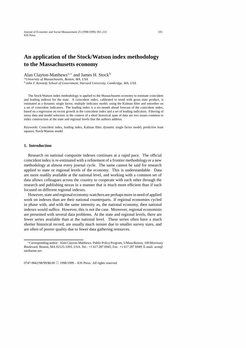
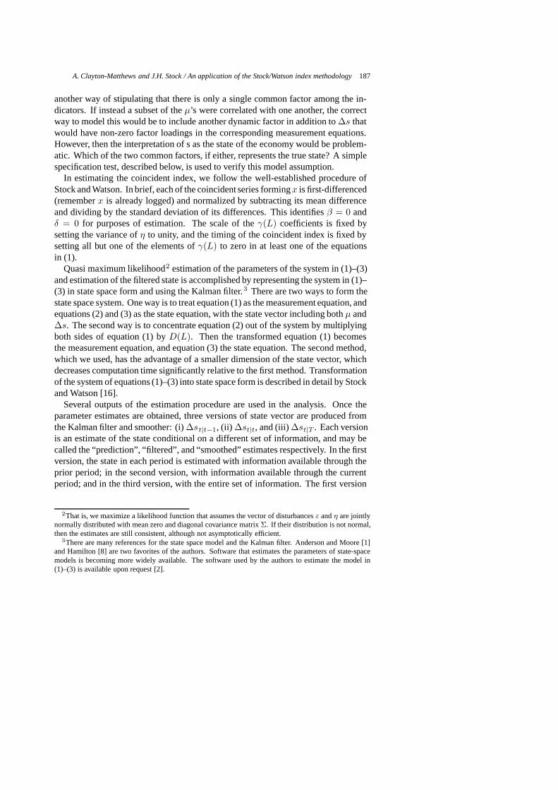
Fig. 1. Transfer functions, by period.
One solution to this problem is to pre-smooth those indicators that are contami-nated with high-frequency noise. Commonly, a weighted moving-average, i.e., non-recursive filter, is used.7 The term “filter” is apt, since each set of moving-averageweights in the time domain corresponds to a transfer function in the frequency do-main that specifies how each frequency of the input series is factored into the outputseries. Frequencies with low factors near zero are filtered out of the input series,while frequencies with factors near one are passed through to the output series. Theuse and specification of filters designed to pass through the frequencies critical forindex formation while filtering out those dominated by noise is an important aspectof index construction. This is especially true for traditional composite methods thatdo not otherwise exploit time-series dynamics.
In the case of the Stock/Watson model that employs the Kalman filter, pre-estimation filtering is not theoretically necessary, because the procedure producesa set of moving-average weights that filter the series over time. Once again, however,pre-estimation filtering is preferred in practice because otherwise the lag polynomialsγ(L) andD(L) in equations (1) and (2) would be of possibly much higher orders,making specification search and estimation much too time-consuming to be practical.
We use two filters for pre-estimation smoothing. One is an optimal bandpass 9-period centered moving average filter, designed to filter out frequen-cies corresponding to periods of less than five months, while letting fre-quencies corresponding to periods of 10 months or more to pass. Thefilter is 1
3.04(−0.216L−4,−0.007L−3, 0.412L−2, 0.831L−1, 1, 0.831L, 0.412L2,−0.007L3,−0.216L4). Its transfer function is graphed in Fig. 1. This filter isused on the two tax-based coincident indicators, which are very noisy at high fre-quencies. Since we use this as a centered moving-average, we require a four-month
7An accessible text explaining the concepts used here, including the design of filters, is Hamming [9].
192 A. Clayton-Matthews and J.H. Stock / An application of the Stock/Watson index methodology
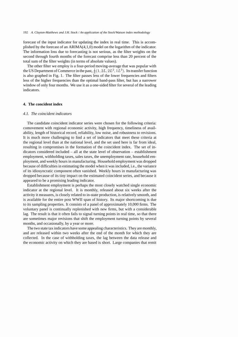
forecast of the input indicator for updating the index in real time. This is accom-plished by the forecast of an ARIMA(4,1,0) model on the logarithm of the indicator.The information loss due to forecasting is not serious, as the filter weights on thesecond through fourth months of the forecast comprise less than 20 percent of thetotal sum of the filter weights (in terms of absolute values).
The other filter we employ is a four-period moving-average that was popular withthe US Department of Commerce in the past,1
6 (1, 2L, 2L2, 1L3). Its transfer functionis also graphed in Fig. 1. The filter passes less of the lower frequencies and filtersless of the higher frequencies than the optimal band-pass filter, but has a narrowerwindow of only four months. We use it as a one-sided filter for several of the leadingindicators.
4. The concident index
4.1. The coincident indicators
The candidate coincident indicator series were chosen for the following criteria:comovement with regional economic activity, high frequency, timeliness of avail-ability, length of historical record, reliability, low noise, and robustness to revisions.It is much more challenging to find a set of indicators that meet these criteria atthe regional level than at the national level, and the set used here is far from ideal,resulting in compromises in the formation of the coincident index. The set of in-dicators considered included – all at the state level of observation – establishmentemployment, withholding taxes, sales taxes, the unemployment rate, household em-ployment, and weekly hours in manufacturing. Household employment was droppedbecause of difficulties in estimating the model when it was included, i.e., the varianceof its idiosyncratic component often vanished. Weekly hours in manufacturing wasdropped because of its tiny impact on the estimated coincident series, and because itappeared to be a promising leading indicator.
Establishment employment is perhaps the most closely watched single economicindicator at the regional level. It is monthly, released about six weeks after theactivity it measures, is closely related to in-state production, is relatively smooth, andis available for the entire post WWII span of history. Its major shortcoming is dueto its sampling properties. It consists of a panel of approximately 10,000 firms. Thevoluntary panel is continually replenished with new firms, but with a considerablelag. The result is that it often fails to signal turning points in real time, so that thereare sometimes major revisions that shift the employment turning points by severalmonths, and occasionally, by a year or more.
The two state tax indicators have some appealing characteristics. They are monthly,and are released within two weeks after the end of the month for which they arecollected. In the case of withholding taxes, the lag between the data release andthe economic activity on which they are based is short. Large companies that remit
A. Clayton-Matthews and J.H. Stock / An application of the Stock/Watson index methodology 193
withholding taxes weekly within days of the end of the pay period account for about85 percent of total withholding taxes. The lag in sales tax collections is roughly amonth longer. Prior to 1998, approximately 70 percent of monthly tax receipts werefor sales made in the current month. However, due to a tax law change, sales taxreceipts for a given month now reflect sales made in the prior month. Perhaps the bestcharacteristic of these tax series is that they are not samples, by virtue of includingall taxpayers.
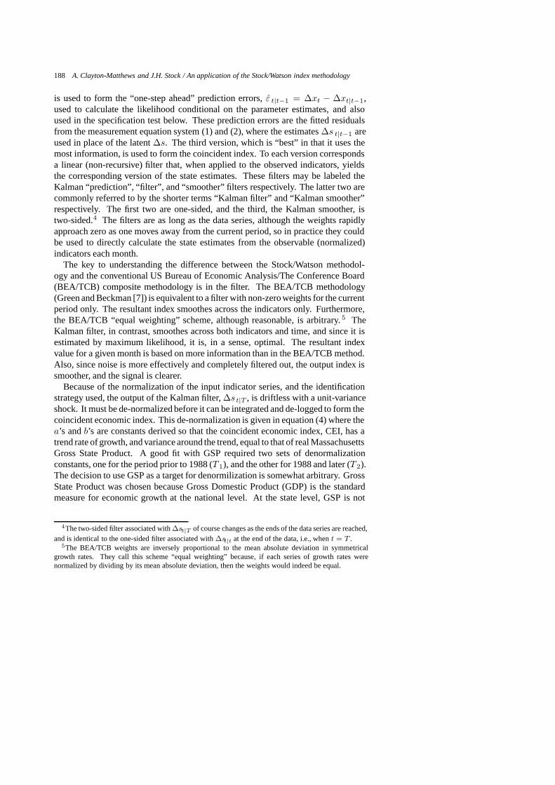
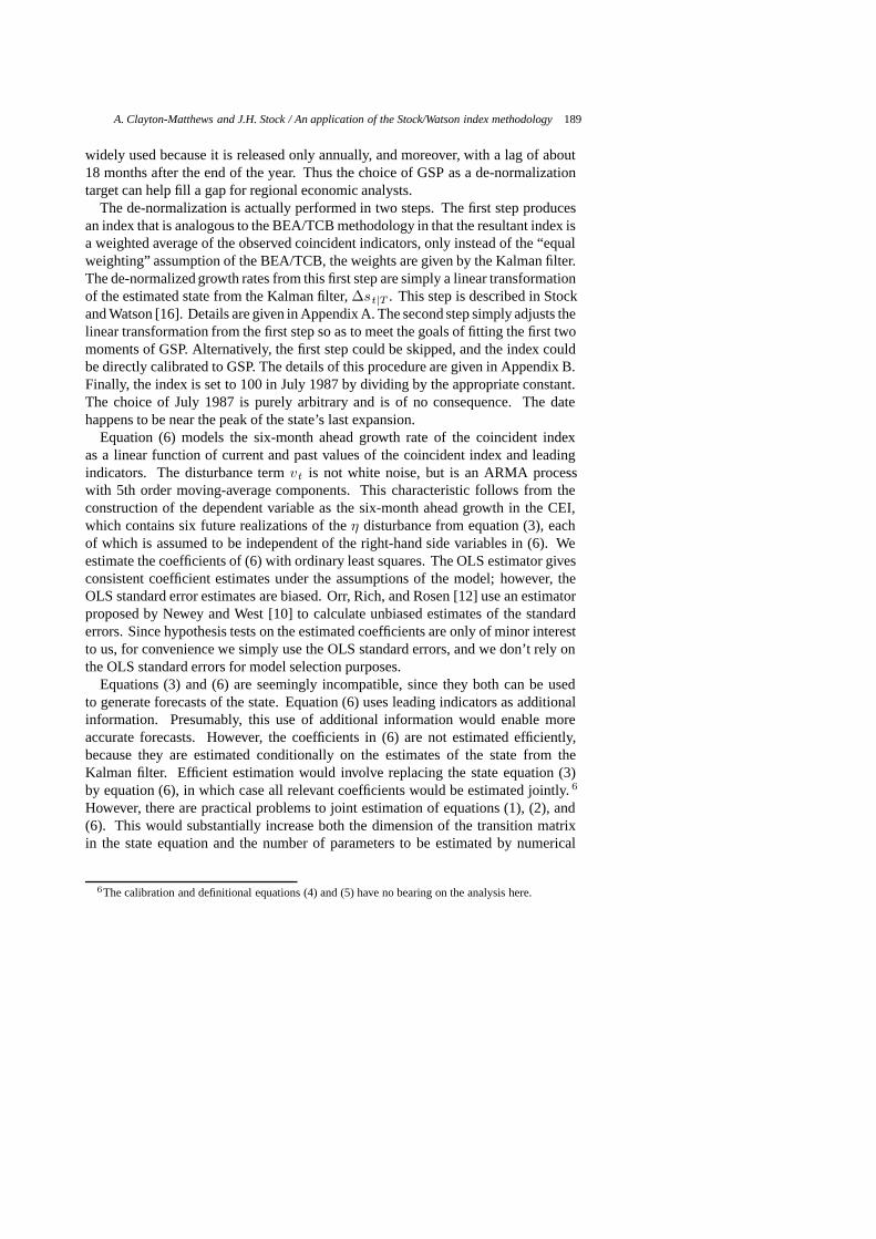
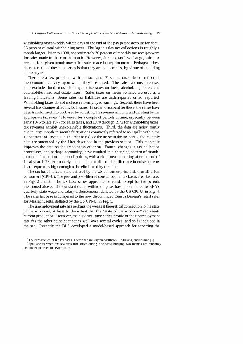
There are a few problems with the tax data. First, the taxes do not reflect allthe economic activity upon which they are based. The sales tax measure usedhere excludes food; most clothing; excise taxes on fuels, alcohol, cigarettes, andautomobiles; and real estate taxes. (Sales taxes on motor vehicles are used as aleading indicator.) Some sales tax liabilities are underreported or not reported.Withholding taxes do not include self-employed earnings. Second, there have beenseveral law changes affecting both taxes. In order to account for these, the series havebeen transformed into tax bases by adjusting the revenue amounts and dividing by theappropriate tax rates.8 However, for a couple of periods of time, especially betweenearly 1976 to late 1977 for sales taxes, and 1970 through 1972 for withholding taxes,tax revenues exhibit unexplainable fluctuations. Third, the data are noisy, partlydue to large month-to-month fluctuations commonly referred to as “spill” within theDepartment of Revenue.9 In order to reduce the noise in the tax series, the monthlydata are smoothed by the filter described in the previous section. This markedlyimproves the data on the smoothness criterion. Fourth, changes in tax collectionprocedures, and perhaps accounting, have resulted in a changing pattern of month-to-month fluctuations in tax collections, with a clear break occurring after the end offiscal year 1978. Fortunately, most – but not all – of the difference in noise patternsis at frequencies high enough to be eliminated by the filter.
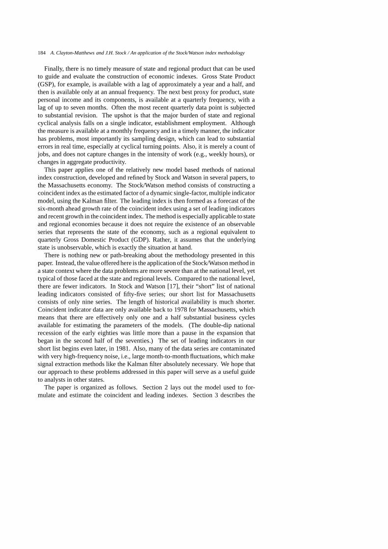
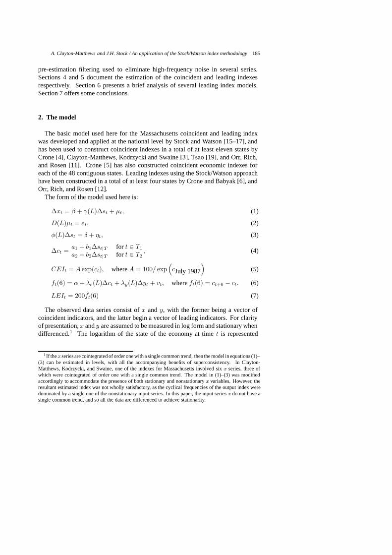
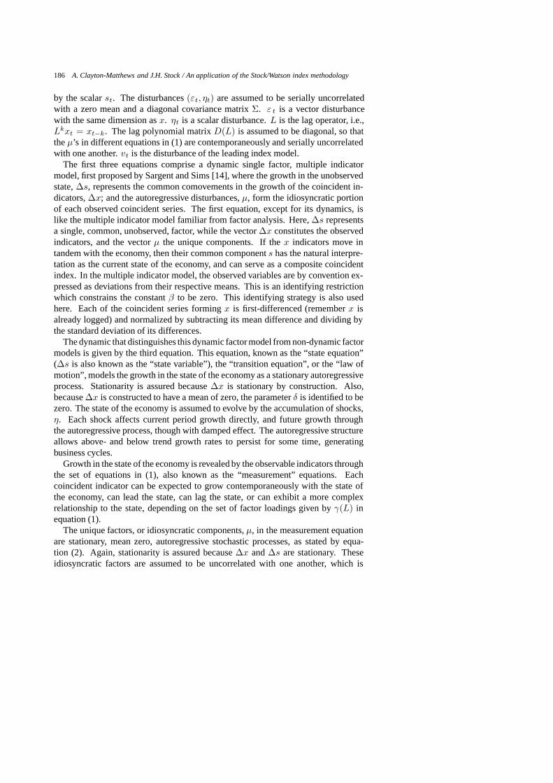
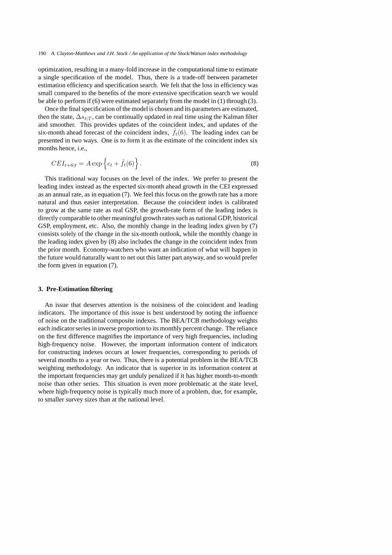
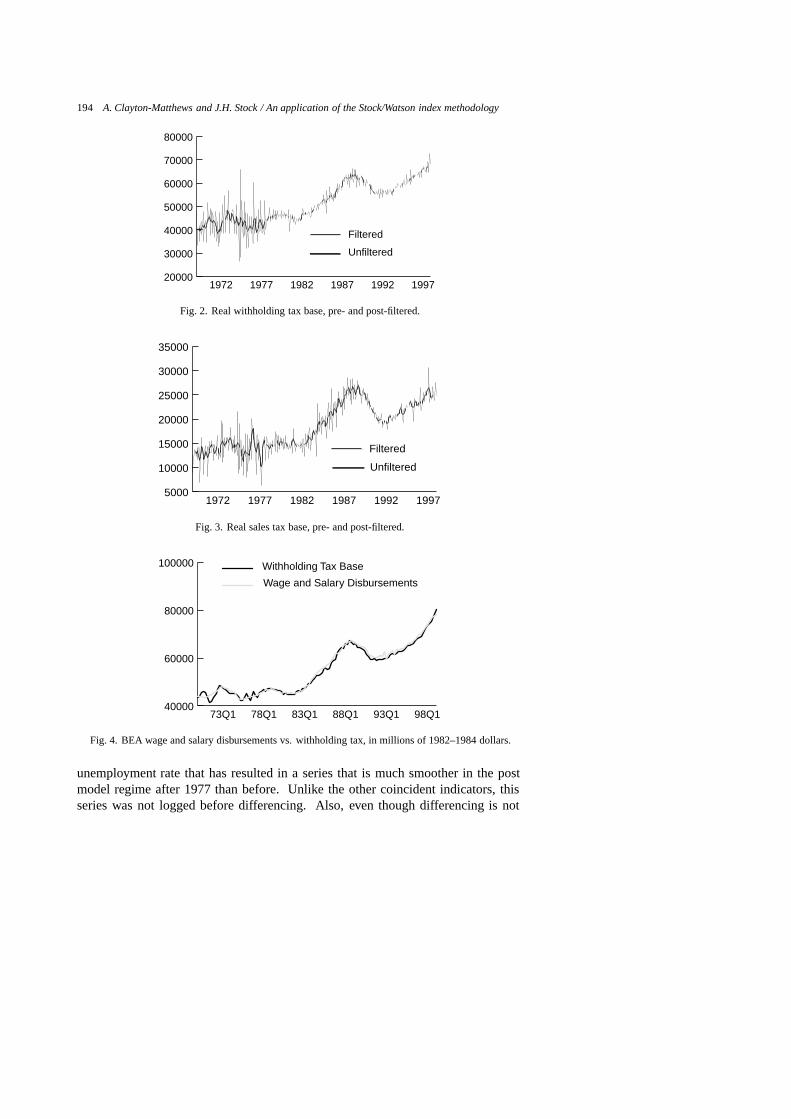
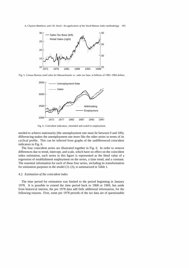
The tax base indicators are deflated by the US consumer price index for all urbanconsumers (CPI-U). The pre- and post-filtered constant dollar tax bases are illustratedin Figs 2 and 3. The tax base series appear to be valid, except for the periodsmentioned above. The constant-dollar withholding tax base is compared to BEA’squarterly state wage and salary disbursements, deflated by the US CPI-U, in Fig. 4.The sales tax base is compared to the now discontinued Census Bureau’s retail salesfor Massachusetts, deflated by the US CPI-U, in Fig. 5.
The unemployment rate has perhaps the weakest theoretical connection to the stateof the economy, at least to the extent that the “state of the economy” representscurrent production. However, the historical time series profile of the unemploymentrate fits the other coincident series well over several cycles, and so is included inthe set. Recently the BLS developed a model-based approach for reporting the
8The construction of the tax bases is described in Clayton-Matthews, Kodrzycki, and Swaine [3].9Spill occurs when tax revenues that arrive during a window bridging two months are randomly
distributed between the two months.
194 A. Clayton-Matthews and J.H. Stock / An application of the Stock/Watson index methodology
20000
30000
40000
50000
60000
70000
80000
Filtered
Unfiltered
199719921987198219771972
Fig. 2. Real withholding tax base, pre- and post-filtered.
5000
10000
15000
20000
25000
30000
35000
Filtered
Unfiltered
199719921987198219771972
Fig. 3. Real sales tax base, pre- and post-filtered.
40000
60000
80000
100000 Withholding Tax Base
Wage and Salary Disbursements
98Q193Q188Q183Q178Q173Q1
Fig. 4. BEA wage and salary disbursements vs. withholding tax, in millions of 1982–1984 dollars.
unemployment rate that has resulted in a series that is much smoother in the postmodel regime after 1977 than before. Unlike the other coincident indicators, thisseries was not logged before differencing. Also, even though differencing is not
A. Clayton-Matthews and J.H. Stock / An application of the Stock/Watson index methodology 195
10
15
20
25
30
25
30
35
40
Retail Sales (right)
Sales Tax Base (left)
199619911986198119761971
Fig. 5. Census Bureau retail sales for Massachusetts vs. sales tax base, in billions of 1982–1984 dollars.
2000
2500
3000
3500 Unemployment Rate
Sales
Withholding
Employment
199719921987198219771972
Fig. 6. Coincident indicators, retrended and scaled to employment.
needed to achieve stationarity (the unemployment rate must lie between 0 and 100),differencing makes the unemployment rate more like the other series in terms of itscyclical profile. This can be inferred from graphs of the undifferenced coincidentindicators in Fig. 6.
The four coincident series are illustrated together in Fig. 6. In order to removedifferences due to trend, intercept, and scale, which have no effect on the coincidentindex estimation, each series in this figure is represented as the fitted value of aregression of establishment employment on the series, a time trend, and a constant.The essential information for each of these four series, including its transformationfor estimation purposes in the model (1)–(3), is summarized in Table 1.
4.2. Estimation of the coincident index
The time period for estimation was limited to the period beginning in January1978. It is possible to extend the time period back to 1968 or 1969, but asidefrom historical interest, the pre 1978 data add little additional information, for thefollowing reasons. First, some pre 1978 periods of the tax data are of questionable
196 A. Clayton-Matthews and J.H. Stock / An application of the Stock/Watson index methodology
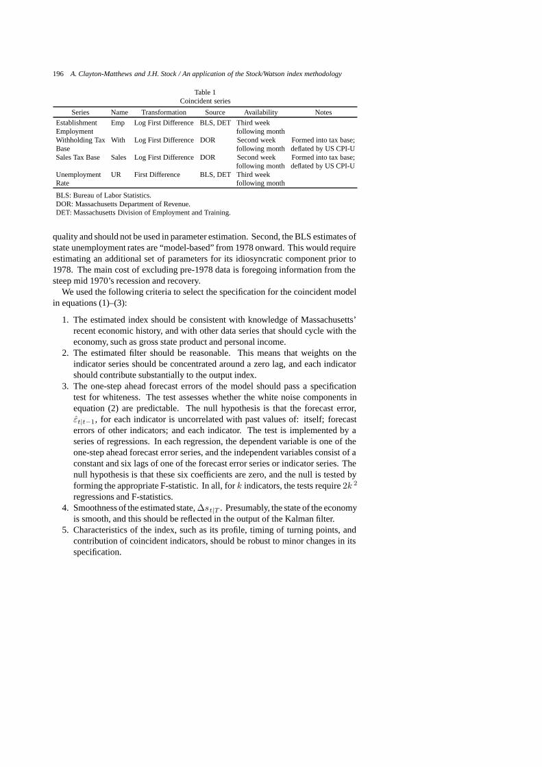
Table 1Coincident series
Series Name Transformation Source Availability Notes
Establishment Emp Log First Difference BLS, DET Third weekEmployment following monthWithholding Tax With Log First Difference DOR Second week Formed into tax base;Base following month deflated by US CPI-USales Tax Base Sales Log First Difference DOR Second week Formed into tax base;
following month deflated by US CPI-UUnemployment UR First Difference BLS, DET Third weekRate following month
BLS: Bureau of Labor Statistics.DOR: Massachusetts Department of Revenue.DET: Massachusetts Division of Employment and Training.
quality and should not be used in parameter estimation. Second, the BLS estimates ofstate unemployment rates are “model-based” from 1978 onward. This would requireestimating an additional set of parameters for its idiosyncratic component prior to1978. The main cost of excluding pre-1978 data is foregoing information from thesteep mid 1970’s recession and recovery.
We used the following criteria to select the specification for the coincident modelin equations (1)–(3):
1. The estimated index should be consistent with knowledge of Massachusetts’recent economic history, and with other data series that should cycle with theeconomy, such as gross state product and personal income.
2. The estimated filter should be reasonable. This means that weights on theindicator series should be concentrated around a zero lag, and each indicatorshould contribute substantially to the output index.
3. The one-step ahead forecast errors of the model should pass a specificationtest for whiteness. The test assesses whether the white noise components inequation (2) are predictable. The null hypothesis is that the forecast error,ε̂t|t−1, for each indicator is uncorrelated with past values of: itself; forecasterrors of other indicators; and each indicator. The test is implemented by aseries of regressions. In each regression, the dependent variable is one of theone-step ahead forecast error series, and the independent variables consist of aconstant and six lags of one of the forecast error series or indicator series. Thenull hypothesis is that these six coefficients are zero, and the null is tested byforming the appropriate F-statistic. In all, fork indicators, the tests require2k 2
regressions and F-statistics.4. Smoothness of the estimated state,∆st|T . Presumably, the state of the economy
is smooth, and this should be reflected in the output of the Kalman filter.5. Characteristics of the index, such as its profile, timing of turning points, and
contribution of coincident indicators, should be robust to minor changes in itsspecification.
A. Clayton-Matthews and J.H. Stock / An application of the Stock/Watson index methodology 197
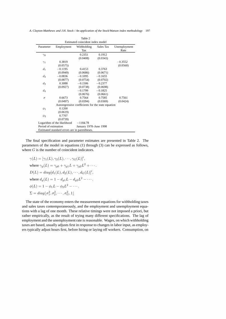
Table 2Estimated coincident index model
Parameter Employment Withholding Sales Tax UnemploymentTax Rate
γ0 0.2351 0.1912(0.0408) (0.0343)
γ1 0.3819 −0.3552(0.0575) (0.0560)
d1 −0.1195 0.4153 0.3763(0.0949) (0.0686) (0.0671)
d2 −0.0836 −0.1095 −0.1655(0.0877) (0.0754) (0.0702)
d3 0.3088 −0.1506 −0.2377(0.0927) (0.0738) (0.0698)
d4 −0.1799 −0.1825(0.0676) (0.0661)
σ 0.6673 0.7564 0.7585 0.7561(0.0497) (0.0394) (0.0369) (0.0424)
Autoregressive coefficients for the state equationφ1 0.1200
(0.0619)φ2 0.7707
(0.0739)Logarithm of the likelihood −1184.78Period of estimation January 1978–June 1998Estimated standard errors are in parentheses.
The final specification and parameter estimates are presented in Table 2. Theparameters of the model in equations (1) through (3) can be expressed as follows,whereG is the number of coincident indicators.
γ(L) = [γ1(L), γ2(L), · · · , γG(L)]′,
whereγg(L) = γg0 + γg1L + γg2L2 + · · · .
D(L) = diag[d1(L), d2(L), · · · , dG(L)]′,
wheredg(L) = 1 − dg1L − dg2L2 − · · · .
φ(L) = 1 − φ1L − φ2L2 − · · · .
Σ = diag�σ21, σ
22 , · · · , σ2
G, 1�
The state of the economy enters the measurement equations for withholding taxesand sales taxes contemporaneously, and the employment and unemployment equa-tions with a lag of one month. These relative timings were not imposed a priori, butrather empirically, as the result of trying many different specifications. The lag ofemployment and the unemployment rate is reasonable. Wages, on which withholdingtaxes are based, usually adjusts first in response to changes in labor input, as employ-ers typically adjust hours first, before hiring or laying off workers. Consumption, on
198 A. Clayton-Matthews and J.H. Stock / An application of the Stock/Watson index methodology
60
80
100
120 Sales
Withholding
Unemployment Rate
EmploymentIndex
19981993198819831978
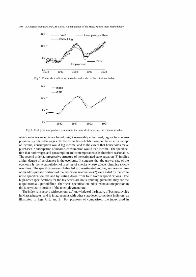
Fig. 7. Conincident indicators, retrended and scaled to the coincident index.
60
80
100
120
GSP
Index
1997199219871982
Fig. 8. Real gross state product, retrended to the coincident index, vs. the coincident index.
which sales tax receipts are based, might reasonably either lead, lag, or be contem-poraneously related to wages. To the extent households make purchases after receiptof income, consumption would lag income, and to the extent that households makepurchases in anticipation of income, consumption would lead income. The specifica-tion that both wages and consumption are contemporaneous is therefore reasonable.The second order autoregressive structure of the estimated state equation (3) impliesa high degree of persistence in the economy. It suggests that the growth rate of theeconomy is the accumulation of a series of shocks whose effects diminish slowlyover time. The specification search that led to the estimated autoregressive structuresof the idiosyncratic portions of the indicators in equation (2) were aided by the whitenoise specification test and by testing down from fourth-order specifications. Thehigh-order specifications for the tax series are not surprising given that they are theoutput from a 9-period filter. The “best” specification indicated no autoregression inthe idiosyncratic portion of the unemployment rate.
The index is in accord with economists’ knowledgeof the history of business cyclesin Massachusetts, and is in agreement with other state-level coincident indictors, asillustrated in Figs 7, 8, and 9. For purposes of comparison, the index used in
A. Clayton-Matthews and J.H. Stock / An application of the Stock/Watson index methodology 199
60
80
100
120
Income
Index
19981993198819831978
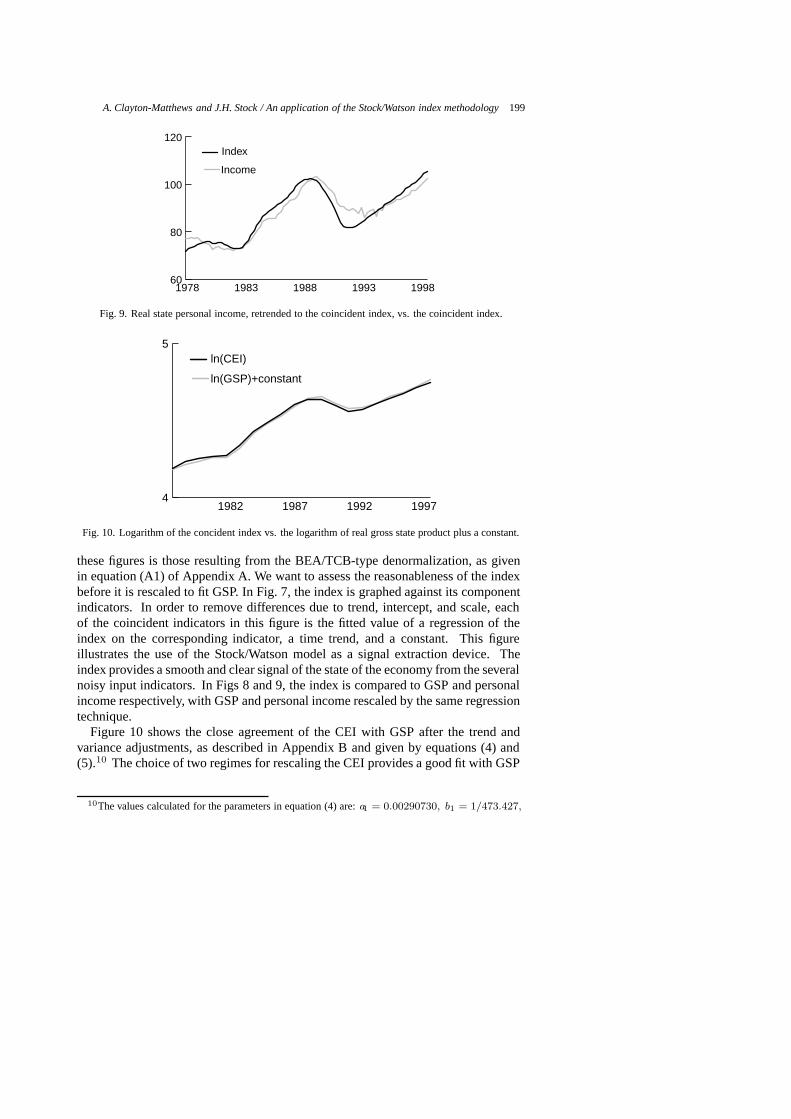
Fig. 9. Real state personal income, retrended to the coincident index, vs. the coincident index.
4
5
ln(GSP)+constant
ln(CEI)
1997199219871982
Fig. 10. Logarithm of the concident index vs. the logarithm of real gross state product plus a constant.
these figures is those resulting from the BEA/TCB-type denormalization, as givenin equation (A1) of Appendix A. We want to assess the reasonableness of the indexbefore it is rescaled to fit GSP. In Fig. 7, the index is graphed against its componentindicators. In order to remove differences due to trend, intercept, and scale, eachof the coincident indicators in this figure is the fitted value of a regression of theindex on the corresponding indicator, a time trend, and a constant. This figureillustrates the use of the Stock/Watson model as a signal extraction device. Theindex provides a smooth and clear signal of the state of the economy from the severalnoisy input indicators. In Figs 8 and 9, the index is compared to GSP and personalincome respectively, with GSP and personal income rescaled by the same regressiontechnique.
Figure 10 shows the close agreement of the CEI with GSP after the trend andvariance adjustments, as described in Appendix B and given by equations (4) and(5).10 The choice of two regimes for rescaling the CEI provides a good fit with GSP
10The values calculated for the parameters in equation (4) are:a1 = 0.00290730, b1 = 1/473.427,
200 A. Clayton-Matthews and J.H. Stock / An application of the Stock/Watson index methodology
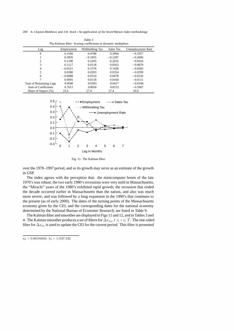
Table 3The Kalman filter: Scoring coefficients or dynamic multipliers
Lag Employment Withholding Tax Sales Tax Unemployment Rate
0 0.1566 0.4788 0.3994 −0.10571 0.3835 −0.1855 −0.1287 −0.26062 0.1190 0.2205 0.2032 −0.04163 0.1117 0.0118 0.0563 −0.08704 −0.0521 0.1576 0.1438 −0.02825 0.0380 0.0203 0.0354 −0.02996 −0.0088 0.0510 0.0478 −0.01437 0.0091 0.0118 0.0164 −0.0111
Sum of Remaining Lags 0.0040 0.0393 0.0417 −0.0184Sum of Coefficients 0.7611 0.8056 0.8153 −0.5967Share of Impact (%) 25.6 27.0 27.4 20.0
-0.3
-0.2
-0.1
0.0
0.1
0.2
0.3
0.4
0.5
Unemployment Rate
Sales Tax
Withholding Tax
Employment
76543210
Lag in Months
Fig. 11. The Kalman filter.
over the 1978–1997 period, and so its growth may serve as an estimate of the growthin GSP.
The index agrees with the perception that: the minicomputer boom of the late1970’s was robust; the two early 1980’s recessions were very mild in Massachusetts;the “Miracle” years of the 1980’s exhibited rapid growth; the recession that endedthe decade occurred earlier in Massachusetts than the nation, and also was muchmore severe; and was followed by a long expansion in the 1990’s that continues tothe present (as of early 2000). The dates of the turning points of the Massachusettseconomy given by the CEI, and the corresponding dates for the national economydetermined by the National Bureau of Economic Research, are listed in Table 9.
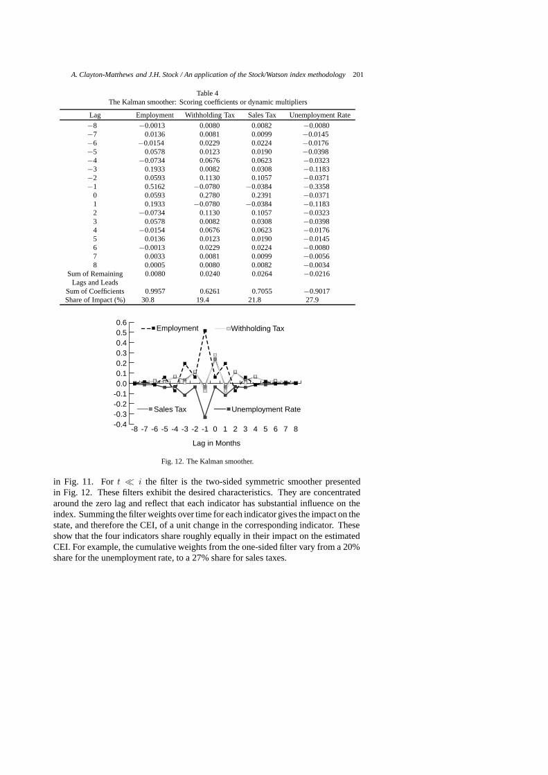
The Kalman filter and smoother are displayed in Figs 11 and 12, and in Tables 3 and4. The Kalman smoother produces a set of filters for∆s t|i, t � i � T . The one-sidedfilter for ∆st|t is used to update the CEI for the current period. This filter is presented
a2 = 0.00194050, b2 = 1/637.332.
A. Clayton-Matthews and J.H. Stock / An application of the Stock/Watson index methodology 201
Table 4The Kalman smoother: Scoring coefficients or dynamic multipliers
Lag Employment Withholding Tax Sales Tax Unemployment Rate
−8 −0.0013 0.0080 0.0082 −0.0080−7 0.0136 0.0081 0.0099 −0.0145−6 −0.0154 0.0229 0.0224 −0.0176−5 0.0578 0.0123 0.0190 −0.0398−4 −0.0734 0.0676 0.0623 −0.0323−3 0.1933 0.0082 0.0308 −0.1183−2 0.0593 0.1130 0.1057 −0.0371−1 0.5162 −0.0780 −0.0384 −0.3358
0 0.0593 0.2780 0.2391 −0.03711 0.1933 −0.0780 −0.0384 −0.11832 −0.0734 0.1130 0.1057 −0.03233 0.0578 0.0082 0.0308 −0.03984 −0.0154 0.0676 0.0623 −0.01765 0.0136 0.0123 0.0190 −0.01456 −0.0013 0.0229 0.0224 −0.00807 0.0033 0.0081 0.0099 −0.00568 0.0005 0.0080 0.0082 −0.0034
Sum of Remaining 0.0080 0.0240 0.0264 −0.0216Lags and Leads
Sum of Coefficients 0.9957 0.6261 0.7055 −0.9017Share of Impact (%) 30.8 19.4 21.8 27.9
-0.4-0.3-0.2-0.10.00.10.20.30.40.50.6
Unemployment RateSales Tax
Withholding TaxEmployment
876543210-1-2-3-4-5-6-7-8
Lag in Months
Fig. 12. The Kalman smoother.
in Fig. 11. Fort � i the filter is the two-sided symmetric smoother presentedin Fig. 12. These filters exhibit the desired characteristics. They are concentratedaround the zero lag and reflect that each indicator has substantial influence on theindex. Summing the filter weights over time for each indicator gives the impact on thestate, and therefore the CEI, of a unit change in the corresponding indicator. Theseshow that the four indicators share roughly equally in their impact on the estimatedCEI. For example, the cumulative weights from the one-sided filter vary from a 20%share for the unemployment rate, to a 27% share for sales taxes.
202 A. Clayton-Matthews and J.H. Stock / An application of the Stock/Watson index methodology
Table 5Whiteness specification test p-values
Regressors: A Constant and Six Lags of: Dependent Variable: One-Step Ahead Forecast Error ofCorresponding Indicator
Employment Withholding Sales Taxes Unemploy-Taxes ment Rate
One-Step Ahead Employment 0.140 0.384 0.731 0.963Forecast Error Withholding Taxes 0.101 0.100 0.120 0.378
Sales Taxes 0.119 0.406 0.583 0.507Unemployment Rate 0.913 0.135 0.673 0.018
Transformed Employment 0.101 0.817 0.720 0.621Indicators (See Withholding Taxes 0.590 0.580 0.645 0.050Table 1 for the Sales Taxes 0.232 0.213 0.856 0.246Transformation) Unemployment Rate 0.004 0.150 0.071 0.066
The entries in the table are the p-values from a regression of the one-step ahead forecast error on a constantand six lags of the indicated regressor. The p-values correspond to the F-test of the null hypothesis thatthe coefficients (except for the constant) are all zero.
60
80
100
120
Complex
Final
19981993198819831978
Fig. 13. Indexes of the final and more complex specifications..
The results of the whiteness specification test are given in Table 5. Only two outof the 32 p-values are less than 0.05, so the specification satisfies this test reasonablywell. If the 32 tests were independent (they’re not), then the probability of two ormore p-values below 0.05 would be 0.48.
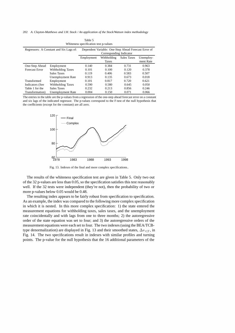
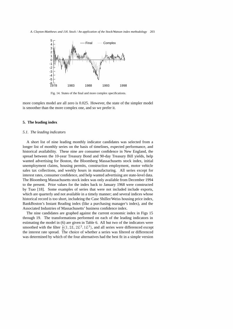
The resulting index appears to be fairly robust from specification to specification.As an example, the index was compared to the following more complex specificationin which it is nested. In this more complex specification: 1) the state entered themeasurement equations for withholding taxes, sales taxes, and the unemploymentrate coincidentally and with lags from one to three months; 2) the autoregressiveorder of the state equation was set to four; and 3) the autoregressive orders of themeasurement equations were each set to four. The two indexes (using the BEA/TCB-type denormalization) are displayed in Fig. 13 and their smoothed states,∆s t|T , inFig. 14. The two specifications result in indexes with similar profiles and turningpoints. The p-value for the null hypothesis that the 16 additional parameters of the
A. Clayton-Matthews and J.H. Stock / An application of the Stock/Watson index methodology 203
-6-5-4-3-2-1012345
ComplexFinal
19981993198819831978
Fig. 14. States of the final and more complex specifications.
more complex model are all zero is 0.025. However, the state of the simpler modelis smoother than the more complex one, and so we prefer it.
5. The leading index
5.1. The leading indicators
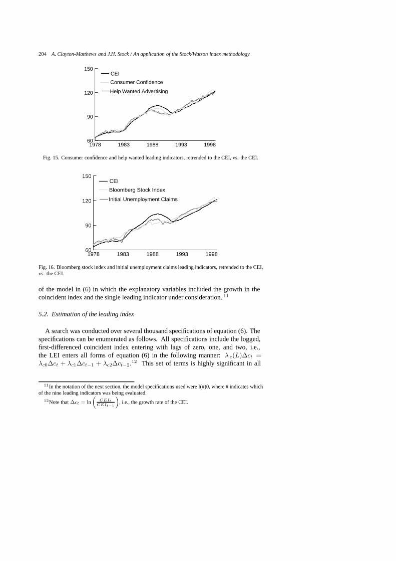
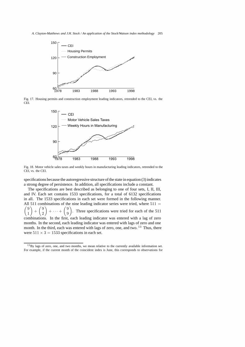
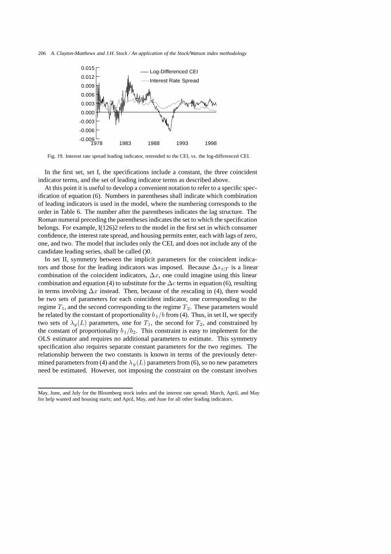
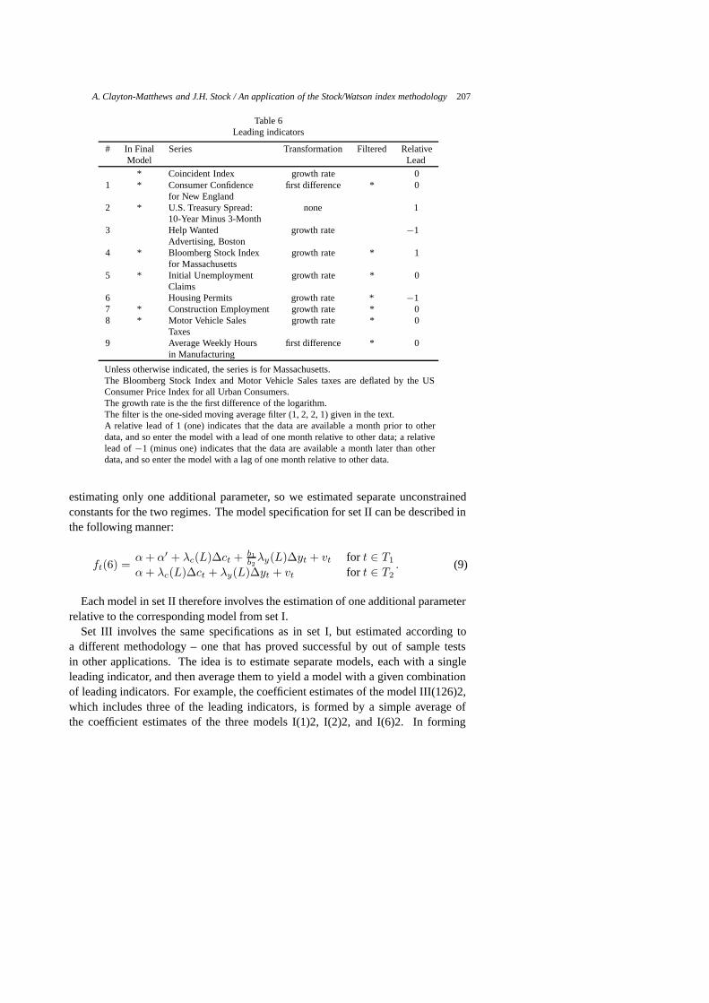
A short list of nine leading monthly indicator candidates was selected from alonger list of monthly series on the basis of timelines, expected performance, andhistorical availability. These nine are consumer confidence in New England, thespread between the 10-year Treasury Bond and 90-day Treasury Bill yields, helpwanted advertising for Boston, the Bloomberg Massachusetts stock index, initialunemployment claims, housing permits, construction employment, motor vehiclesales tax collections, and weekly hours in manufacturing. All series except forinterest rates, consumer confidence, and help wanted advertising are state-level data.The Bloomberg Massachusetts stock index was only available from December 1994to the present. Prior values for the index back to January 1968 were constructedby Tsao [18]. Some examples of series that were not included include exports,which are quarterly and not available in a timely manner; and several indices whosehistorical record is too short, includeing the Case Shiller/Weiss housing price index,BankBoston’s Instant Reading index (like a purchasing manager’s index), and theAssociated Industries of Massachusetts’ business confidence index.
The nine candidates are graphed against the current economic index in Figs 15through 19. The transformations performed on each of the leading indicators inestimating the model in (6) are given in Table 6. All but two of the indicators weresmoothed with the filter1
6 (1, 2L, 2L2, 1L3), and all series were differenced exceptthe interest rate spread. The choice of whether a series was filtered or differencedwas determined by which of the four alternatives had the best fit in a simple version
204 A. Clayton-Matthews and J.H. Stock / An application of the Stock/Watson index methodology
60
90
120
150
Help Wanted Advertising
Consumer Confidence
CEI
19981993198819831978
Fig. 15. Consumer confidence and help wanted leading indicators, retrended to the CEI, vs. the CEI.
60
90
120
150
Initial Unemployment Claims
Bloomberg Stock Index
CEI
19981993198819831978
Fig. 16. Bloomberg stock index and initial unemployment claims leading indicators, retrended to the CEI,vs. the CEI.
of the model in (6) in which the explanatory variables included the growth in thecoincident index and the single leading indicator under consideration.11
5.2. Estimation of the leading index
A search was conducted over several thousand specifications of equation (6). Thespecifications can be enumerated as follows. All specifications include the logged,first-differenced coincident index entering with lags of zero, one, and two, i.e.,the LEI enters all forms of equation (6) in the following manner:λ c(L)∆ct =λc0∆ct + λc1∆ct−1 + λc2∆ct−2.12 This set of terms is highly significant in all
11In the notation of the next section, the model specifications used were I(#)0, where # indicates whichof the nine leading indicators was being evaluated.
12Note that∆ct = ln(
CEItCEIt−1
), i.e., the growth rate of the CEI.
A. Clayton-Matthews and J.H. Stock / An application of the Stock/Watson index methodology 205
60
90
120
150
Construction Employment
Housing Permits
CEI
19981993198819831978
Fig. 17. Housing permits and construction employment leading indicators, retrended to the CEI, vs. theCEI.
60
90
120
150
Weekly Hours in Manufacturing
Motor Vehicle Sales Taxes
CEI
19981993198819831978
Fig. 18. Motor vehicle sales taxes and weekly hours in manufacturing leading indicators, retrended to theCEI, vs. the CEI.
specifications because the autoregressive structure of the state in equation (3) indicatesa strong degree of persistence. In addition, all specifications include a constant.
The specifications are best described as belonging to one of four sets, I, II, III,and IV. Each set contains 1533 specifications, for a total of 6132 specificationsin all. The 1533 specifications in each set were formed in the following manner.All 511 combinations of the nine leading indicator series were tried, where511 =(
91
)+
(92
)+ · · · +
(99
). Three specifications were tried for each of the 511
combinations. In the first, each leading indicator was entered with a lag of zeromonths. In the second, each leading indicator was entered with lags of zero and onemonth. In the third, each was entered with lags of zero, one, and two.13 Thus, therewere511 × 3 = 1533 specifications in each set.
13By lags of zero, one, and two months, we mean relative to the currently available information set.For example, if the current month of the coincident index is June, this corresponds to observations for
206 A. Clayton-Matthews and J.H. Stock / An application of the Stock/Watson index methodology
-0.009
-0.006
-0.003
0.000
0.003
0.006
0.009
0.012
0.015
Interest Rate Spread
Log-Differenced CEI
19981993198819831978
Fig. 19. Interest rate spread leading indicator, retrended to the CEI, vs. the log-differenced CEI.
In the first set, set I, the specifications include a constant, the three coincidentindicator terms, and the set of leading indicator terms as described above.
At this point it is useful to develop a convenient notation to refer to a specific spec-ification of equation (6). Numbers in parentheses shall indicate which combinationof leading indicators is used in the model, where the numbering corresponds to theorder in Table 6. The number after the parentheses indicates the lag structure. TheRoman numeral preceding the parentheses indicates the set to which the specificationbelongs. For example, I(126)2 refers to the model in the first set in which consumerconfidence, the interest rate spread, and housing permits enter, each with lags of zero,one, and two. The model that includes only the CEI, and does not include any of thecandidate leading series, shall be called ()0.
In set II, symmetry between the implicit parameters for the coincident indica-tors and those for the leading indicators was imposed. Because∆s t|T is a linearcombination of the coincident indicators,∆x, one could imagine using this linearcombination and equation (4) to substitute for the∆c terms in equation (6), resultingin terms involving∆x instead. Then, because of the rescaling in (4), there wouldbe two sets of parameters for each coincident indicator, one corresponding to theregimeT1, and the second corresponding to the regimeT 2. These parameters wouldbe related by the constant of proportionalityb1/b from (4). Thus, in set II, we specifytwo sets ofλy(L) parameters, one forT1, the second forT2, and constrained bythe constant of proportionalityb1/b2. This constraint is easy to implement for theOLS estimator and requires no additional parameters to estimate. This symmetryspecification also requires separate constant parameters for the two regimes. Therelationship between the two constants is known in terms of the previously deter-mined parameters from (4) and theλy(L) parameters from (6), so no new parametersneed be estimated. However, not imposing the constraint on the constant involves
May, June, and July for the Bloomberg stock index and the interest rate spread; March, April, and Mayfor help wanted and housing starts; and April, May, and June for all other leading indicators.
A. Clayton-Matthews and J.H. Stock / An application of the Stock/Watson index methodology 207
Table 6Leading indicators
# In Final Series Transformation Filtered RelativeModel Lead
* Coincident Index growth rate 01 * Consumer Confidence first difference * 0
for New England2 * U.S. Treasury Spread: none 1
10-Year Minus 3-Month3 Help Wanted growth rate −1
Advertising, Boston4 * Bloomberg Stock Index growth rate * 1
for Massachusetts5 * Initial Unemployment growth rate * 0
Claims6 Housing Permits growth rate * −17 * Construction Employment growth rate * 08 * Motor Vehicle Sales growth rate * 0
Taxes9 Average Weekly Hours first difference * 0
in Manufacturing
Unless otherwise indicated, the series is for Massachusetts.The Bloomberg Stock Index and Motor Vehicle Sales taxes are deflated by the USConsumer Price Index for all Urban Consumers.The growth rate is the the first difference of the logarithm.The filter is the one-sided moving average filter (1, 2, 2, 1) given in the text.A relative lead of 1 (one) indicates that the data are available a month prior to otherdata, and so enter the model with a lead of one month relative to other data; a relativelead of−1 (minus one) indicates that the data are available a month later than otherdata, and so enter the model with a lag of one month relative to other data.
estimating only one additional parameter, so we estimated separate unconstrainedconstants for the two regimes. The model specification for set II can be described inthe following manner:
ft(6) =α + α′ + λc(L)∆ct + b1
b2λy(L)∆yt + vt for t ∈ T1
α + λc(L)∆ct + λy(L)∆yt + vt for t ∈ T2. (9)
Each model in set II therefore involves the estimation of one additional parameterrelative to the corresponding model from set I.
Set III involves the same specifications as in set I, but estimated according toa different methodology – one that has proved successful by out of sample testsin other applications. The idea is to estimate separate models, each with a singleleading indicator, and then average them to yield a model with a given combinationof leading indicators. For example, the coefficient estimates of the model III(126)2,which includes three of the leading indicators, is formed by a simple average ofthe coefficient estimates of the three models I(1)2, I(2)2, and I(6)2. In forming
208 A. Clayton-Matthews and J.H. Stock / An application of the Stock/Watson index methodology
these averages, excluded leading indicators implicitly have a coefficient of zero.14
Averaging the coefficients of the models is equivalent to averaging their predicted orfitted values.
Set IV applies the same estimation strategy used in set III to the specifications ofset II. For example, the coefficient estimates of the model IV(126)2, is formed bya simple average of the coefficient estimates of the three models II(1)2, II(2)2, andII(6)2.
Each specification was ranked on the basis of several criteria. These included thefollowing:
1. Predictive least squares (PLS) sum of squared residuals (lower is better). Thiscriterion ranks specifications on the basis of the cumulative sum of squaresof six-step ahead forecast errors, also known as recursive residuals. For thelinear regression modelyt = b′xt + εt, the criterion selects the regressorx
that minimizesPLS(x) =T∑
t=s
(yt0 − b′t−kxt)2, wherebi is the least squares
estimate based ont � i, and wheres is great enough so that the estimated insample residuals from the estimation ofbs have positive degrees of freedom.15
We setk = 6 (rather thank = 1) because the dependent variable is the six-month ahead growth rate of theCEI. The PLS procedure we used reflected, asmuch as conveniently possible, real time updating of the coefficient estimatesof b and the estimation ofyt. For example, in constructing the tax baseseach month, which required applying a filter centered on the current month,appropriate forecasts were made, rather than using actual historical data. Wedid not, however, attempt to reproduce the actual, pre-revised, data that wouldhave been available each month. Nor did we reestimate the parameters of thecoincident index model (1)–(4) each month.
2. Lowest value of the Bayesian Information Criterion (BIC) (lower is better).
The measure isBIC = ln(
SSRT
)+ K
(lnTT
), whereSSR is the sum of
squared residuals of the regression,T is the number of observations, andKis the number of parameters in the model. The BIC rewards fit but penalizesfor complexity. Wei [20] showed that, for ergodic models, PLS and BIC are
14We also tried a variant of this method where an additional regression was run that only included thecoincident index terms, and the regressions for each leading indicator did not include the coincident indexterms. This variant did not perform as well, because the averaging of coefficients diluted the effect of thebest predictor, the coincident index.
15The choice of s is arbitrary, but does affect the result. A straightforward standard is to select theminimum s possible. However, as Wei [20] notes, the early prediction errors in this case may be quitelarge and have too much influence on the result. We chose a value ofs that was six years (72 observations)into the observation range, which allowed recursive residuals to be calculated over a period of time thatspanned the last two turning points. yet allowed at least 40 degrees of freedom for the most parameterizedmodel.
A. Clayton-Matthews and J.H. Stock / An application of the Stock/Watson index methodology 209
asymptotically equivalent, although in practice the two measures can yield quitedifferent results.
3. Highest share of contribution due to the leading indicators (higher is better).The share of an indicator is defined to be the weighted sum of its coefficientsfrom (6),divided by the weighted sum for all indicators, including the coincidentindex. The sign for initial unemployment claims is appropriately reversed. Theweight for an indicator’s coefficients is the standard deviation of the year-over-year change in the indicator. The purpose of this weighting is to standardize thecoefficients for typical changes in the indicators at business cycle frequencies.Because of the high persistence of the state in equation (3), the coincidentindicator consistently accounts for the largest share, which was well over halfin all 6132 specifications. This criterion favors those specifications in whichthe leading indicators, as a group, have the most influence on the forecast ofthe coincident index.
4. Equality of shares of the leading indicators (more equal is better). Consideringonly the leading indicators, this measure is the average absolute deviation ofthe indicator share from the average share of all the leading indicators, wherethe shares are defined as above.16
5. The number of leading indicators (more is better).6. The number of “wrong” signs on the leading indicators (fewer are better). The
sign of an indicator is defined to be the sign of the sum of its coefficients whenit enters with one or more lags. The sign is expected to be positive for all of theindicators except initial unemployment claims.
Interestingly, the rankings based on the PLS and the BIC criteria are differentin several respects, according to some basic characteristics of the top 100 modelsaccording to each of the two criteria. First, only two models are in both top 100rankings. Second, half the top 100 PLS models are from set I and half are fromset II, while all expect one of the top 100 BIC models are from set II. The extraconstant parameter for the regime dummy is almost always significant, but thatdoesn’t necessarily lead to the best out of sample performance. The top models bythe PLS criterion are more complex than those that score highest on the BIC. All thePLS models include two lags of the leading indicators, while only a few of the BICmodels include any lags at all (except two lags of the CEI, which all models include).The top models by PLS also contain slightly more leading indicators on average, 4.96versus 4.44 for the top models by the BIC. The leading indicators contribute a largershare, on average, of the variation in the index (criterion number three above) in thetop PLS models than in the top BIC models, 29 percent versus 18 percent. This isnot surprising given their relative complexity. However, there are more wrong signsin the top PLS models. Weekly hours in manufacturing have the wrong sign in all
16In calculating the average the divisor is the number of leading indicators in the specification lessone-half to offset a bias in this measure infavor of specifications with few indicators.
210 A. Clayton-Matthews and J.H. Stock / An application of the Stock/Watson index methodology
66 of the top 100 PLS models in which they enter, and help wanted advertising hasthe wrong sign in all 41 of the top 100 PLS models in which they enter. Among thetop 100 BIC models, 22 have weekly hours entering with the wrong sign (in onlyone model does it enters with the right sign), and 12 have construction employmententering with the wrong sign (9 have construction employment with the right sign).No other indicators enter any of these 198 models with the wrong signs. Threeleading indicators occur frequently in both lists. Consumer confidence appears in alltop 100 PLS models and 66 of the top 100 BIC models. The Bloomberg stock indexappears in all top 100 BIC models and in 60 of the top PLS models. Motor vehiclesales taxes appear in all PLS models and 54 BIC models. No other indicators entermore than half the models of both lists. However, the interest rate spread enters 63of the BIC models, and 30 of the PLS models; and weekly hours in manufacturingenters 66 of the PLS models, but with the wrong sign as previously mentioned.
None of the models from sets III or IV were in either of the top 100 lists, andtherefore did not fit or predict as well as their multivariate counterparts.
These distinctly different rankings by the PLS and BIC are part of the reason forincluding the other criteria in model selection. However, an even more importantconsideration is the short time period over which the leading indicator models arefit. Given data availability, the estimation period is July 1981 through April 1998.Although this consists of 202 monthly observations, it includes essentially only onefull cycle and part of another: the rapid expansion of the “Massachusetts Miracle”years, the steep and long recession that followed, and the long and steady expansionof the 1990’s. Models that either fit well or that perform well in out of sampleforecasts over this short period of time are not guaranteed to perform better in thefuture than models that do not score as well on the PLS or BIC criteria.
The additional four selection criteria are based on the common sense idea that themore indicators contributing to the index, the better. Having a large set of indicatorswhere none is dominant serves as insurance against a mistake in model selection dueto peculiarities of the short historical period on which the models were estimated.Of course, the criterion that favors more indicators introduces the risk of includingseries that are not reliable leading indicators. Our way of guarding for this risk wasto initially narrow down the list to a reasonable set of nine candidate indicators.
To aid us in applying these multidimensional criteria, we eliminated those modelsfrom consideration that contained wrong signs according to the last criterion, andweighted the other criteria equally, except for double weighting the PLS criterion.This served as guide to help narrow down the models into a manageable handfulwhere application of the criteria by subjective judgment, i.e., expert opinion, led tochoosing a “best” model.
6. Analysis of the leading index models
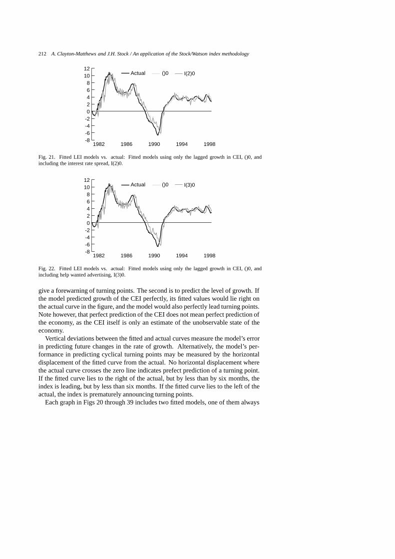
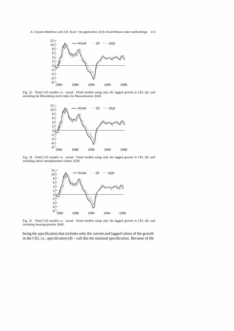
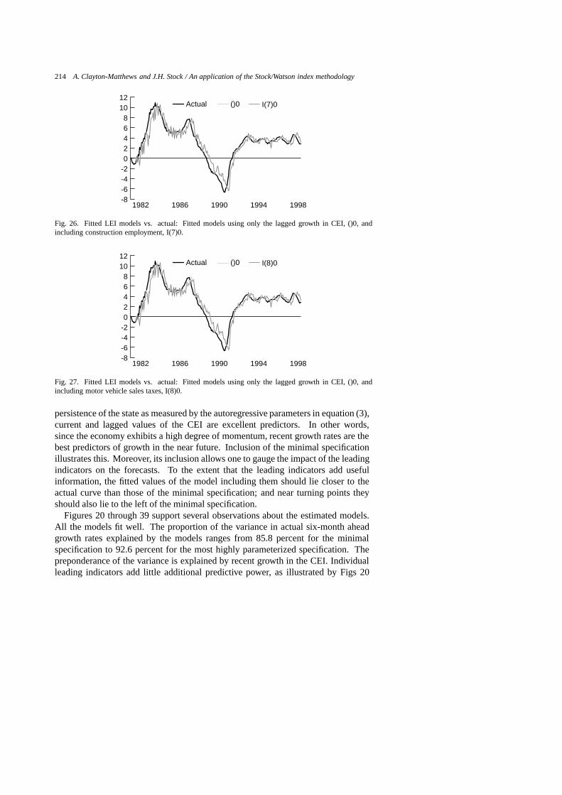
The fitted and actual six-month-ahead growth rates of the CEI for several leadingindex specifications are displayed in Figs 20 through 39, and a guide to these figures
A. Clayton-Matthews and J.H. Stock / An application of the Stock/Watson index methodology 211
Table 7Guide to figures of selected models
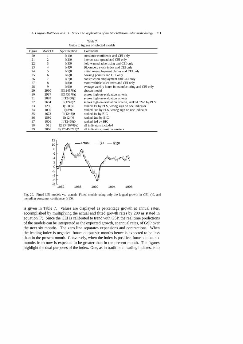
Figure Model # Specification Comments
20 1 I(1)0 consumer confidence and CEI only21 2 I(2)0 interest rate spread and CEI only22 3 I(3)0 help wanted advertising and CEI only23 4 I(4)0 Bloomberg stock index and CEI only24 5 I(5)0 initial unemployment claims and CEI only25 6 I(6)0 housing permits and CEI only26 7 I(7)0 construction employment and CEI only27 8 I(8)0 motor vehicle sales taxes and CEI only28 9 I(9)0 average weekly hours in manufacturing and CEI only29 2960 II(124578)2 chosen model30 2987 II(145678)2 scores high on evaluation criteria31 2828 II(12458)2 scores high on evaluation criteria32 2694 II(1248)2 scores high on evaluation criteria, ranked 52nd by PLS33 1206 I(1689)2 ranked 1st by PLS, wrong sign on one indicator34 1095 I(189)2 ranked 2nd by PLS, wrong sign on one indicator35 1672 II(1248)0 ranked 1st by BIC36 1580 II(124)0 ranked 2nd by BIC37 1806 II(12458)0 ranked 3rd by BIC38 511 I(123456789)0 all indicators included39 3066 II(123456789)2 all indicators, most parameters
-8-6-4-202468
1012
I(1)0()0Actual
19981994199019861982
Fig. 20. Fitted LEI models vs. actual: Fitted models using only the lagged growth in CEI, ()0, andincluding consumer confidence, I(1)0.
is given in Table 7. Values are displayed as percentage growth at annual rates,accomplished by multiplying the actual and fitted growth rates by 200 as stated inequation (7). Since the CEI is calibrated to trend with GSP, the real time predictionsof the models can be interpreted as the expected growth, at annual rates, of GSP overthe next six months. The zero line separates expansions and contractions. Whenthe leading index is negative, future output six months hence is expected to be lessthan in the present month. Conversely, when the index is positive, future output sixmonths from now is expected to be greater than in the present month. The figureshighlight the dual purposes of the index. One, as in traditional leading indexes, is to
212 A. Clayton-Matthews and J.H. Stock / An application of the Stock/Watson index methodology
-8-6-4-202468
1012
I(2)0()0Actual
19981994199019861982
Fig. 21. Fitted LEI models vs. actual: Fitted models using only the lagged growth in CEI, ()0, andincluding the interest rate spread, I(2)0.
-8-6-4-202468
1012
I(3)0()0Actual
19981994199019861982
Fig. 22. Fitted LEI models vs. actual: Fitted models using only the lagged growth in CEI, ()0, andincluding help wanted advertising, I(3)0.
give a forewarning of turning points. The second is to predict the level of growth. Ifthe model predicted growth of the CEI perfectly, its fitted values would lie right onthe actual curve in the figure, and the model would also perfectly lead turning points.Note however, that perfect prediction of the CEI does not mean perfect prediction ofthe economy, as the CEI itself is only an estimate of the unobservable state of theeconomy.
Vertical deviations between the fitted and actual curves measure the model’s errorin predicting future changes in the rate of growth. Alternatively, the model’s per-formance in predicting cyclical turning points may be measured by the horizontaldisplacement of the fitted curve from the actual. No horizontal displacement wherethe actual curve crosses the zero line indicates prefect prediction of a turning point.If the fitted curve lies to the right of the actual, but by less than by six months, theindex is leading, but by less than six months. If the fitted curve lies to the left of theactual, the index is prematurely announcing turning points.
Each graph in Figs 20 through 39 includes two fitted models, one of them always
A. Clayton-Matthews and J.H. Stock / An application of the Stock/Watson index methodology 213
-8-6-4-202468
1012
I(4)0()0Actual
19981994199019861982
Fig. 23. Fitted LEI models vs. actual: Fitted models using only the lagged growth in CEI, ()0, andincluding the Bloomberg stock index for Massachusetts, I(4)0.
-8-6-4-202468
1012
I(5)0()0Actual
19981994199019861982
Fig. 24. Fitted LEI models vs. actual: Fitted models using only the lagged growth in CEI, ()0, andincluding initial unemployment claims, I(5)0.
-8-6-4-202468
1012
I(6)0()0Actual
19981994199019861982
Fig. 25. Fitted LEI models vs. actual: Fitted models using only the lagged growth in CEI, ()0, andincluding housing permits, I(6)0.
being the specification that includes only the current and lagged values of the growthin the CEI, i.e., specification ()0 – call this the minimal specification. Because of the
214 A. Clayton-Matthews and J.H. Stock / An application of the Stock/Watson index methodology
-8-6-4-202468
1012
I(7)0()0Actual
19981994199019861982
Fig. 26. Fitted LEI models vs. actual: Fitted models using only the lagged growth in CEI, ()0, andincluding construction employment, I(7)0.
-8-6-4-202468
1012
I(8)0()0Actual
19981994199019861982
Fig. 27. Fitted LEI models vs. actual: Fitted models using only the lagged growth in CEI, ()0, andincluding motor vehicle sales taxes, I(8)0.
persistence of the state as measured by the autoregressive parameters in equation (3),current and lagged values of the CEI are excellent predictors. In other words,since the economy exhibits a high degree of momentum, recent growth rates are thebest predictors of growth in the near future. Inclusion of the minimal specificationillustrates this. Moreover, its inclusion allows one to gauge the impact of the leadingindicators on the forecasts. To the extent that the leading indicators add usefulinformation, the fitted values of the model including them should lie closer to theactual curve than those of the minimal specification; and near turning points theyshould also lie to the left of the minimal specification.
Figures 20 through 39 support several observations about the estimated models.All the models fit well. The proportion of the variance in actual six-month aheadgrowth rates explained by the models ranges from 85.8 percent for the minimalspecification to 92.6 percent for the most highly parameterized specification. Thepreponderance of the variance is explained by recent growth in the CEI. Individualleading indicators add little additional predictive power, as illustrated by Figs 20
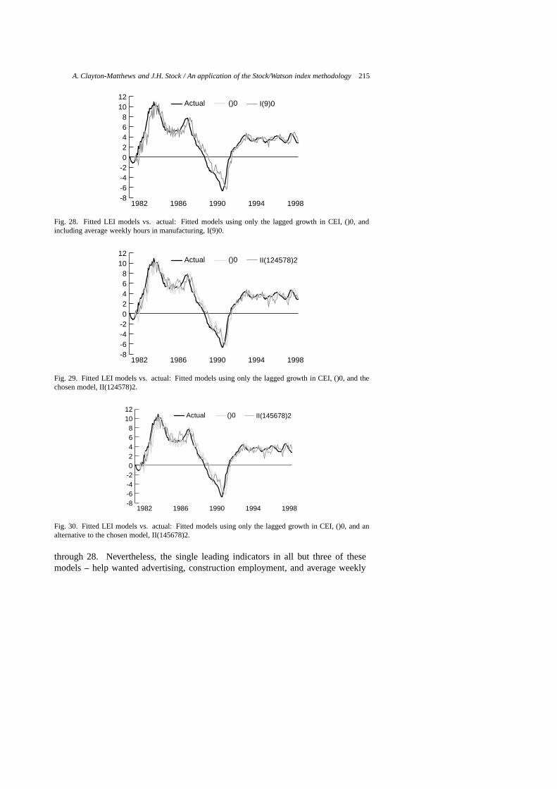
A. Clayton-Matthews and J.H. Stock / An application of the Stock/Watson index methodology 215
-8-6-4-202468
1012
I(9)0()0Actual
19981994199019861982
Fig. 28. Fitted LEI models vs. actual: Fitted models using only the lagged growth in CEI, ()0, andincluding average weekly hours in manufacturing, I(9)0.
-8-6-4-202468
1012
II(124578)2()0Actual
19981994199019861982
Fig. 29. Fitted LEI models vs. actual: Fitted models using only the lagged growth in CEI, ()0, and thechosen model, II(124578)2.
-8-6-4-202468
1012
II(145678)2()0Actual
19981994199019861982
Fig. 30. Fitted LEI models vs. actual: Fitted models using only the lagged growth in CEI, ()0, and analternative to the chosen model, II(145678)2.
through 28. Nevertheless, the single leading indicators in all but three of thesemodels – help wanted advertising, construction employment, and average weekly
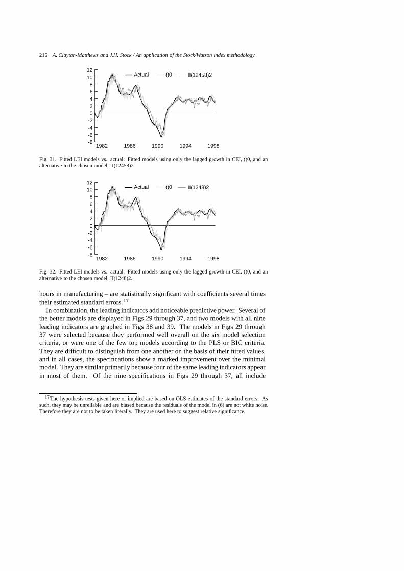
216 A. Clayton-Matthews and J.H. Stock / An application of the Stock/Watson index methodology
-8-6-4-202468
1012
II(12458)2()0Actual
19981994199019861982
Fig. 31. Fitted LEI models vs. actual: Fitted models using only the lagged growth in CEI, ()0, and analternative to the chosen model, II(12458)2.
-8-6-4-202468
1012
II(1248)2()0Actual
19981994199019861982
Fig. 32. Fitted LEI models vs. actual: Fitted models using only the lagged growth in CEI, ()0, and analternative to the chosen model, II(1248)2.
hours in manufacturing – are statistically significant with coefficients several timestheir estimated standard errors.17
In combination, the leading indicators add noticeable predictive power. Several ofthe better models are displayed in Figs 29 through 37, and two models with all nineleading indicators are graphed in Figs 38 and 39. The models in Figs 29 through37 were selected because they performed well overall on the six model selectioncriteria, or were one of the few top models according to the PLS or BIC criteria.They are difficult to distinguish from one another on the basis of their fitted values,and in all cases, the specifications show a marked improvement over the minimalmodel. They are similar primarily because four of the same leading indicators appearin most of them. Of the nine specifications in Figs 29 through 37, all include
17The hypothesis tests given here or implied are based on OLS estimates of the standard errors. Assuch, they may be unreliable and are biased because the residuals of the model in (6) are not white noise.Therefore they are not to be taken literally. They are used here to suggest relative significance.
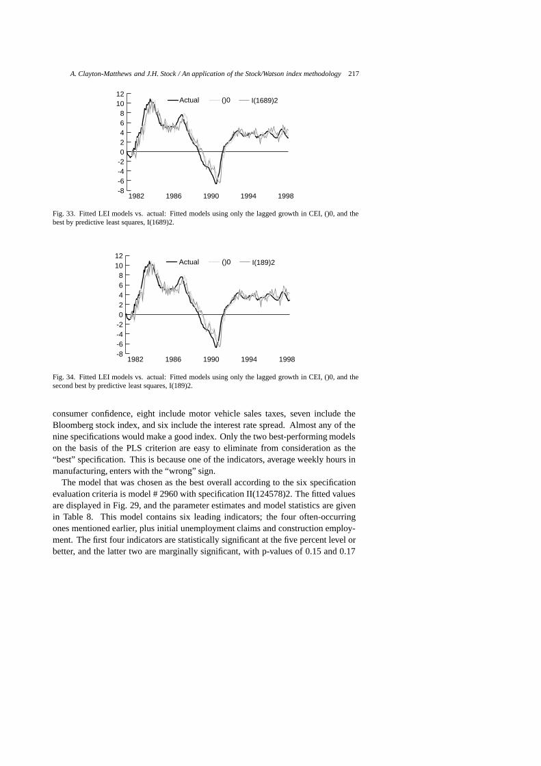
A. Clayton-Matthews and J.H. Stock / An application of the Stock/Watson index methodology 217
-8-6-4-202468
1012
I(1689)2()0Actual
19981994199019861982
Fig. 33. Fitted LEI models vs. actual: Fitted models using only the lagged growth in CEI, ()0, and thebest by predictive least squares, I(1689)2.
-8-6-4-202468
1012
I(189)2()0Actual
19981994199019861982
Fig. 34. Fitted LEI models vs. actual: Fitted models using only the lagged growth in CEI, ()0, and thesecond best by predictive least squares, I(189)2.
consumer confidence, eight include motor vehicle sales taxes, seven include theBloomberg stock index, and six include the interest rate spread. Almost any of thenine specifications would make a good index. Only the two best-performing modelson the basis of the PLS criterion are easy to eliminate from consideration as the“best” specification. This is because one of the indicators, average weekly hours inmanufacturing, enters with the “wrong” sign.
The model that was chosen as the best overall according to the six specificationevaluation criteria is model # 2960 with specification II(124578)2. The fitted valuesare displayed in Fig. 29, and the parameter estimates and model statistics are givenin Table 8. This model contains six leading indicators; the four often-occurringones mentioned earlier, plus initial unemployment claims and construction employ-ment. The first four indicators are statistically significant at the five percent level orbetter, and the latter two are marginally significant, with p-values of 0.15 and 0.17
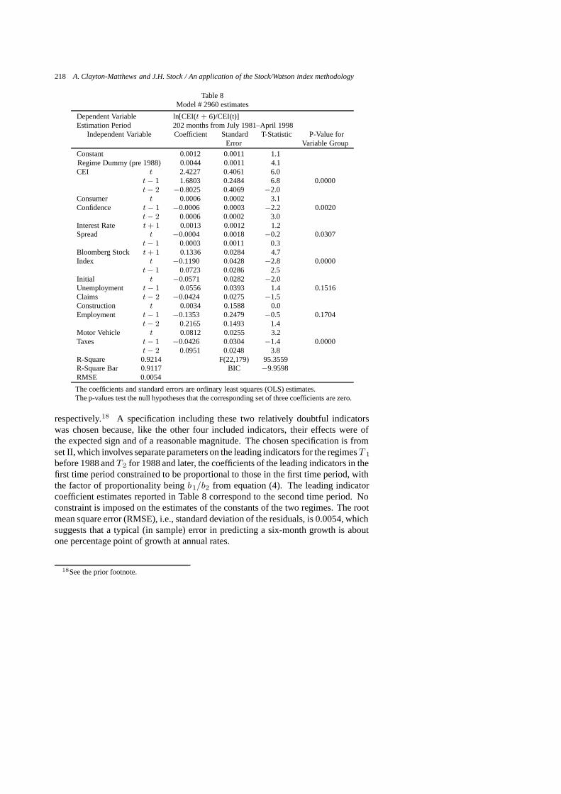
218 A. Clayton-Matthews and J.H. Stock / An application of the Stock/Watson index methodology
Table 8Model # 2960 estimates
Dependent Variable ln[CEI(t + 6)/CEI(t)]Estimation Period 202 months from July 1981–April 1998
Independent Variable Coefficient Standard T-Statistic P-Value forError Variable Group
Constant 0.0012 0.0011 1.1Regime Dummy (pre 1988) 0.0044 0.0011 4.1CEI t 2.4227 0.4061 6.0
t − 1 1.6803 0.2484 6.8 0.0000t − 2 −0.8025 0.4069 −2.0
Consumer t 0.0006 0.0002 3.1Confidence t − 1 −0.0006 0.0003 −2.2 0.0020
t − 2 0.0006 0.0002 3.0Interest Rate t + 1 0.0013 0.0012 1.2Spread t −0.0004 0.0018 −0.2 0.0307
t − 1 0.0003 0.0011 0.3Bloomberg Stock t + 1 0.1336 0.0284 4.7Index t −0.1190 0.0428 −2.8 0.0000
t − 1 0.0723 0.0286 2.5Initial t −0.0571 0.0282 −2.0Unemployment t − 1 0.0556 0.0393 1.4 0.1516Claims t − 2 −0.0424 0.0275 −1.5Construction t 0.0034 0.1588 0.0Employment t − 1 −0.1353 0.2479 −0.5 0.1704
t − 2 0.2165 0.1493 1.4Motor Vehicle t 0.0812 0.0255 3.2Taxes t − 1 −0.0426 0.0304 −1.4 0.0000
t − 2 0.0951 0.0248 3.8R-Square 0.9214 F(22,179) 95.3559R-Square Bar 0.9117 BIC −9.9598RMSE 0.0054
The coefficients and standard errors are ordinary least squares (OLS) estimates.The p-values test the null hypotheses that the corresponding set of three coefficients are zero.
respectively.18 A specification including these two relatively doubtful indicatorswas chosen because, like the other four included indicators, their effects were ofthe expected sign and of a reasonable magnitude. The chosen specification is fromset II, which involves separate parameters on the leading indicators for the regimesT 1
before 1988 andT2 for 1988 and later, the coefficients of the leading indicators in thefirst time period constrained to be proportional to those in the first time period, withthe factor of proportionality beingb1/b2 from equation (4). The leading indicatorcoefficient estimates reported in Table 8 correspond to the second time period. Noconstraint is imposed on the estimates of the constants of the two regimes. The rootmean square error (RMSE), i.e., standard deviation of the residuals, is 0.0054, whichsuggests that a typical (in sample) error in predicting a six-month growth is aboutone percentage point of growth at annual rates.
18See the prior footnote.
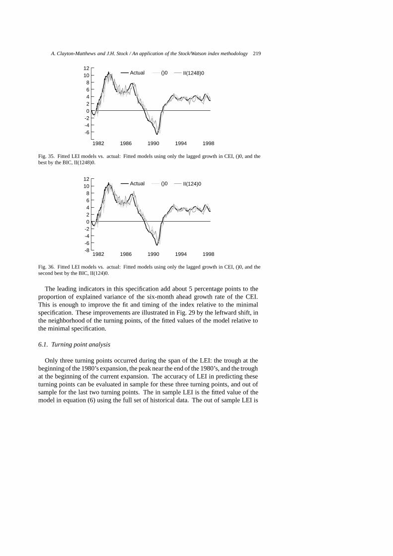
A. Clayton-Matthews and J.H. Stock / An application of the Stock/Watson index methodology 219
-6-4-202468
1012
II(1248)0()0Actual
19981994199019861982
Fig. 35. Fitted LEI models vs. actual: Fitted models using only the lagged growth in CEI, ()0, and thebest by the BIC, II(1248)0.
-8-6-4-202468
1012
II(124)0()0Actual
19981994199019861982
Fig. 36. Fitted LEI models vs. actual: Fitted models using only the lagged growth in CEI, ()0, and thesecond best by the BIC, II(124)0.
The leading indicators in this specification add about 5 percentage points to theproportion of explained variance of the six-month ahead growth rate of the CEI.This is enough to improve the fit and timing of the index relative to the minimalspecification. These improvements are illustrated in Fig. 29 by the leftward shift, inthe neighborhood of the turning points, of the fitted values of the model relative tothe minimal specification.
6.1. Turning point analysis
Only three turning points occurred during the span of the LEI: the trough at thebeginning of the 1980’s expansion, the peak near the end of the 1980’s, and the troughat the beginning of the current expansion. The accuracy of LEI in predicting theseturning points can be evaluated in sample for these three turning points, and out ofsample for the last two turning points. The in sample LEI is the fitted value of themodel in equation (6) using the full set of historical data. The out of sample LEI is
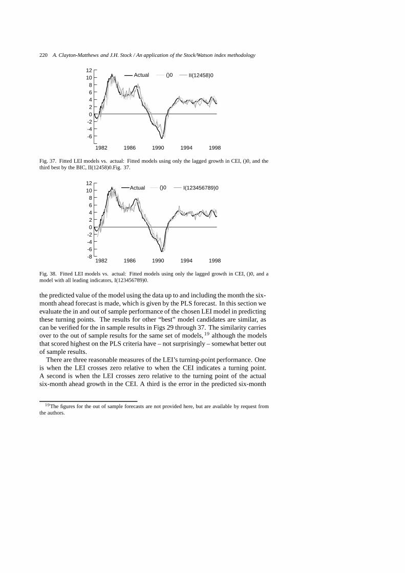
220 A. Clayton-Matthews and J.H. Stock / An application of the Stock/Watson index methodology
-6-4-202468
1012
II(12458)0()0Actual
19981994199019861982
Fig. 37. Fitted LEI models vs. actual: Fitted models using only the lagged growth in CEI, ()0, and thethird best by the BIC, II(12458)0.Fig. 37.
-8-6-4-202468
1012
I(123456789)0()0Actual
19981994199019861982
Fig. 38. Fitted LEI models vs. actual: Fitted models using only the lagged growth in CEI, ()0, and amodel with all leading indicators, I(123456789)0.
the predicted value of the model using the data up to and including the month the six-month ahead forecast is made, which is given by the PLS forecast. In this section weevaluate the in and out of sample performance of the chosen LEI model in predictingthese turning points. The results for other “best” model candidates are similar, ascan be verified for the in sample results in Figs 29 through 37. The similarity carriesover to the out of sample results for the same set of models,19 although the modelsthat scored highest on the PLS criteria have – not surprisingly – somewhat better outof sample results.
There are three reasonable measures of the LEI’s turning-point performance. Oneis when the LEI crosses zero relative to when the CEI indicates a turning point.A second is when the LEI crosses zero relative to the turning point of the actualsix-month ahead growth in the CEI. A third is the error in the predicted six-month
19The figures for the out of sample forecasts are not provided here, but are available by request fromthe authors.
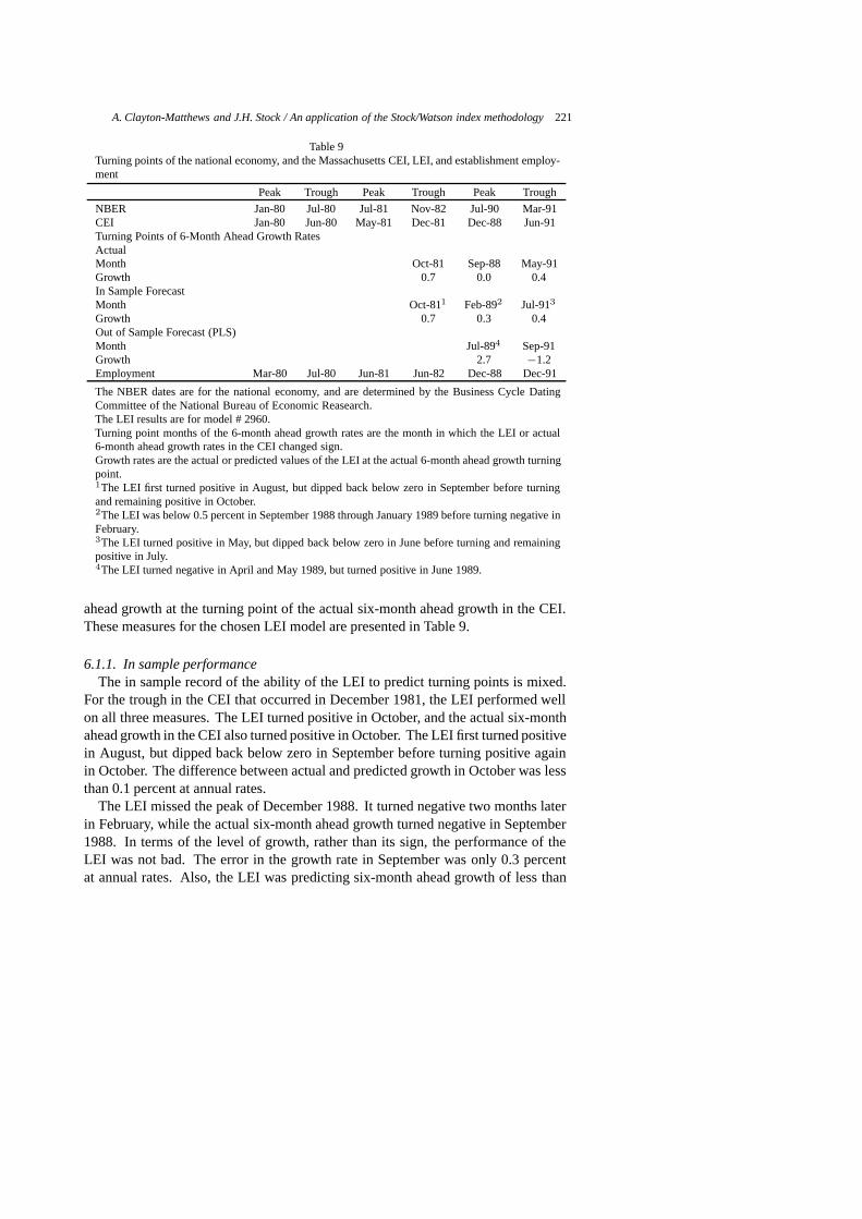
A. Clayton-Matthews and J.H. Stock / An application of the Stock/Watson index methodology 221
Table 9Turning points of the national economy, and the Massachusetts CEI, LEI, and establishment employ-ment
Peak Trough Peak Trough Peak Trough
NBER Jan-80 Jul-80 Jul-81 Nov-82 Jul-90 Mar-91CEI Jan-80 Jun-80 May-81 Dec-81 Dec-88 Jun-91Turning Points of 6-Month Ahead Growth RatesActualMonth Oct-81 Sep-88 May-91Growth 0.7 0.0 0.4In Sample ForecastMonth Oct-811 Feb-892 Jul-913
Growth 0.7 0.3 0.4Out of Sample Forecast (PLS)Month Jul-894 Sep-91Growth 2.7 −1.2Employment Mar-80 Jul-80 Jun-81 Jun-82 Dec-88 Dec-91
The NBER dates are for the national economy, and are determined by the Business Cycle DatingCommittee of the National Bureau of Economic Reasearch.The LEI results are for model # 2960.Turning point months of the 6-month ahead growth rates are the month in which the LEI or actual6-month ahead growth rates in the CEI changed sign.Growth rates are the actual or predicted values of the LEI at the actual 6-month ahead growth turningpoint.1The LEI first turned positive in August, but dipped back below zero in September before turningand remaining positive in October.2The LEI was below 0.5 percent in September 1988 through January 1989 before turning negative inFebruary.3The LEI turned positive in May, but dipped back below zero in June before turning and remainingpositive in July.4The LEI turned negative in April and May 1989, but turned positive in June 1989.
ahead growth at the turning point of the actual six-month ahead growth in the CEI.These measures for the chosen LEI model are presented in Table 9.
6.1.1. In sample performanceThe in sample record of the ability of the LEI to predict turning points is mixed.
For the trough in the CEI that occurred in December 1981, the LEI performed wellon all three measures. The LEI turned positive in October, and the actual six-monthahead growth in the CEI also turned positive in October. The LEI first turned positivein August, but dipped back below zero in September before turning positive againin October. The difference between actual and predicted growth in October was lessthan 0.1 percent at annual rates.
The LEI missed the peak of December 1988. It turned negative two months laterin February, while the actual six-month ahead growth turned negative in September1988. In terms of the level of growth, rather than its sign, the performance of theLEI was not bad. The error in the growth rate in September was only 0.3 percentat annual rates. Also, the LEI was predicting six-month ahead growth of less than
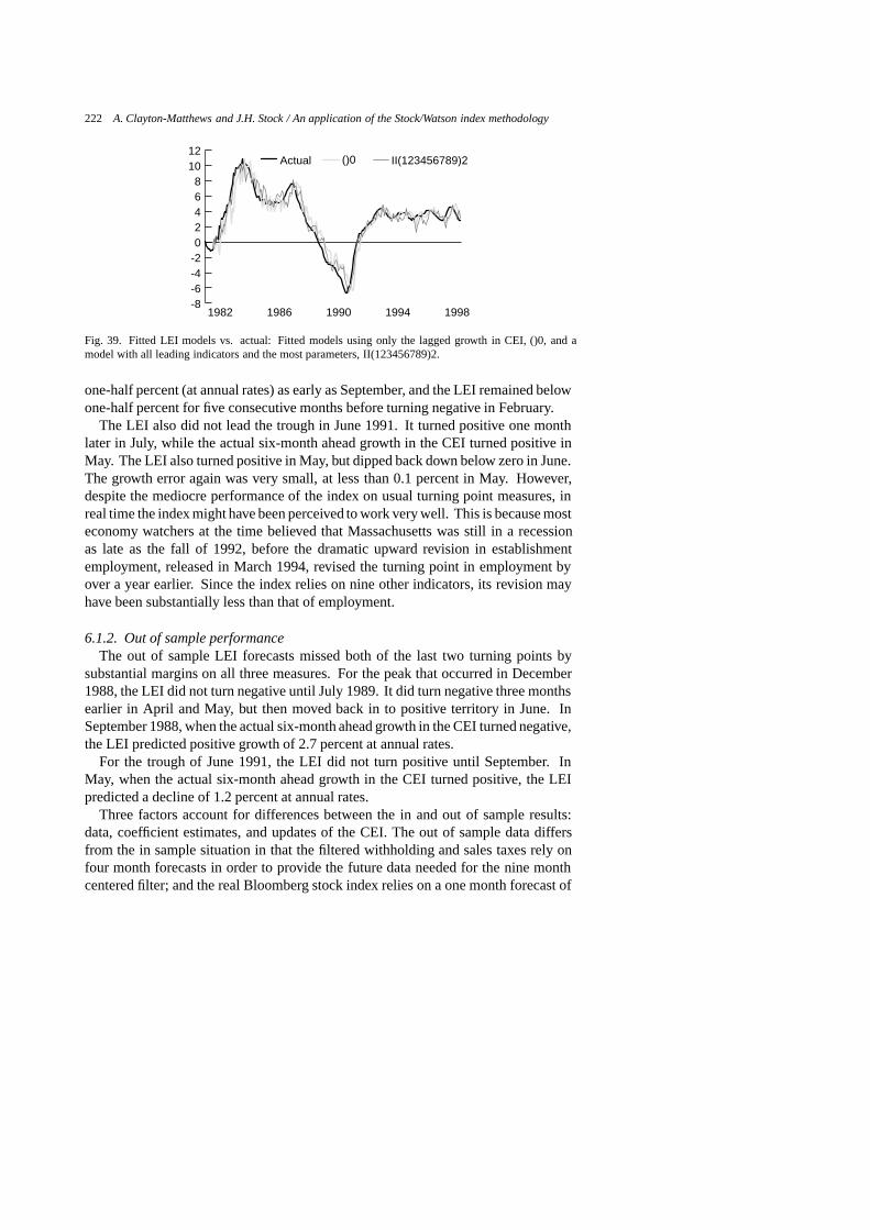
222 A. Clayton-Matthews and J.H. Stock / An application of the Stock/Watson index methodology
-8-6-4-202468
1012
II(123456789)2()0Actual
19981994199019861982
Fig. 39. Fitted LEI models vs. actual: Fitted models using only the lagged growth in CEI, ()0, and amodel with all leading indicators and the most parameters, II(123456789)2.
one-half percent (at annual rates) as early as September, and the LEI remained belowone-half percent for five consecutive months before turning negative in February.
The LEI also did not lead the trough in June 1991. It turned positive one monthlater in July, while the actual six-month ahead growth in the CEI turned positive inMay. The LEI also turned positive in May, but dipped back down below zero in June.The growth error again was very small, at less than 0.1 percent in May. However,despite the mediocre performance of the index on usual turning point measures, inreal time the index might have been perceived to work very well. This is because mosteconomy watchers at the time believed that Massachusetts was still in a recessionas late as the fall of 1992, before the dramatic upward revision in establishmentemployment, released in March 1994, revised the turning point in employment byover a year earlier. Since the index relies on nine other indicators, its revision mayhave been substantially less than that of employment.
6.1.2. Out of sample performanceThe out of sample LEI forecasts missed both of the last two turning points by
substantial margins on all three measures. For the peak that occurred in December1988, the LEI did not turn negative until July 1989. It did turn negative three monthsearlier in April and May, but then moved back in to positive territory in June. InSeptember 1988, when the actual six-month ahead growth in the CEI turned negative,the LEI predicted positive growth of 2.7 percent at annual rates.
For the trough of June 1991, the LEI did not turn positive until September. InMay, when the actual six-month ahead growth in the CEI turned positive, the LEIpredicted a decline of 1.2 percent at annual rates.
Three factors account for differences between the in and out of sample results:data, coefficient estimates, and updates of the CEI. The out of sample data differsfrom the in sample situation in that the filtered withholding and sales taxes rely onfour month forecasts in order to provide the future data needed for the nine monthcentered filter; and the real Bloomberg stock index relies on a one month forecast of
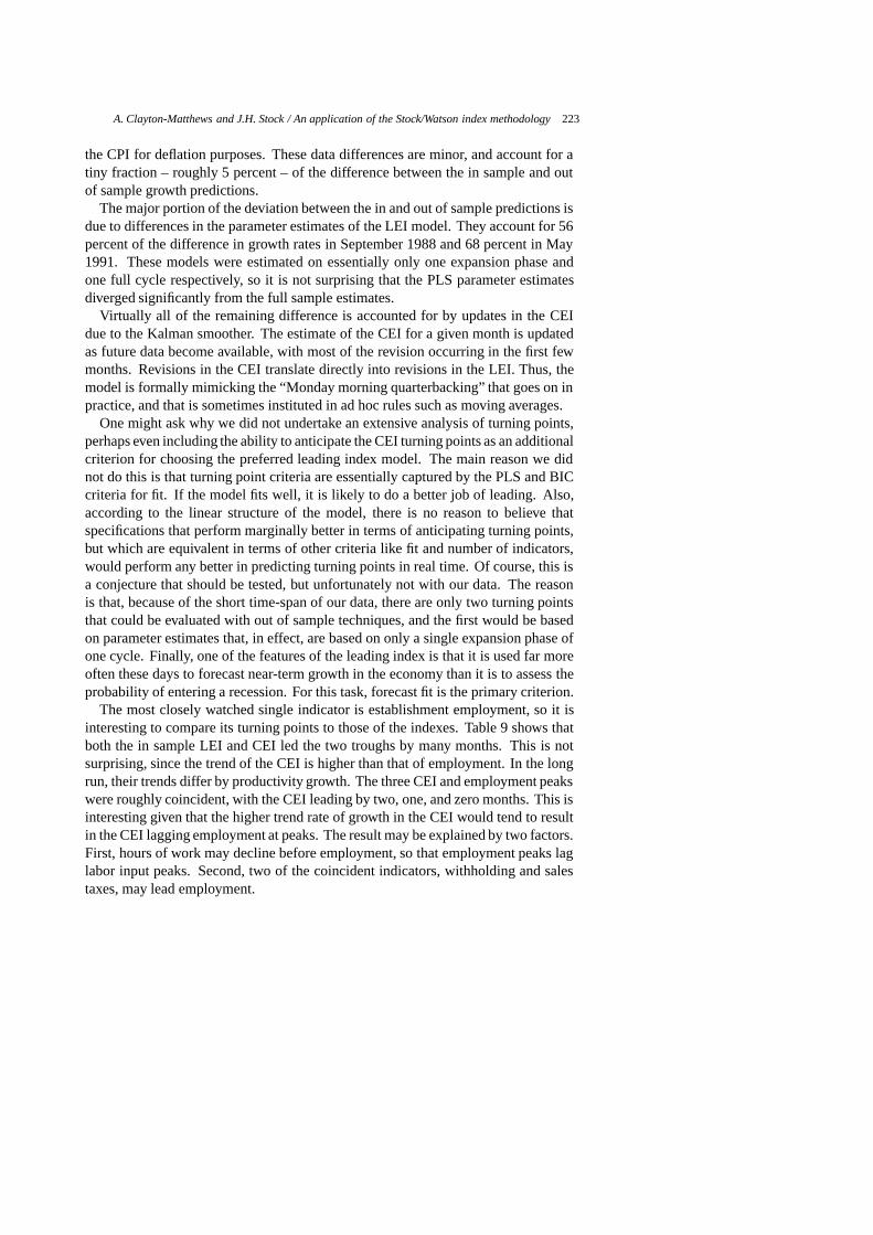
A. Clayton-Matthews and J.H. Stock / An application of the Stock/Watson index methodology 223
the CPI for deflation purposes. These data differences are minor, and account for atiny fraction – roughly 5 percent – of the difference between the in sample and outof sample growth predictions.
The major portion of the deviation between the in and out of sample predictions isdue to differences in the parameter estimates of the LEI model. They account for 56percent of the difference in growth rates in September 1988 and 68 percent in May1991. These models were estimated on essentially only one expansion phase andone full cycle respectively, so it is not surprising that the PLS parameter estimatesdiverged significantly from the full sample estimates.
Virtually all of the remaining difference is accounted for by updates in the CEIdue to the Kalman smoother. The estimate of the CEI for a given month is updatedas future data become available, with most of the revision occurring in the first fewmonths. Revisions in the CEI translate directly into revisions in the LEI. Thus, themodel is formally mimicking the “Monday morning quarterbacking” that goes on inpractice, and that is sometimes instituted in ad hoc rules such as moving averages.
One might ask why we did not undertake an extensive analysis of turning points,perhaps even including the ability to anticipate the CEI turning points as an additionalcriterion for choosing the preferred leading index model. The main reason we didnot do this is that turning point criteria are essentially captured by the PLS and BICcriteria for fit. If the model fits well, it is likely to do a better job of leading. Also,according to the linear structure of the model, there is no reason to believe thatspecifications that perform marginally better in terms of anticipating turning points,but which are equivalent in terms of other criteria like fit and number of indicators,would perform any better in predicting turning points in real time. Of course, this isa conjecture that should be tested, but unfortunately not with our data. The reasonis that, because of the short time-span of our data, there are only two turning pointsthat could be evaluated with out of sample techniques, and the first would be basedon parameter estimates that, in effect, are based on only a single expansion phase ofone cycle. Finally, one of the features of the leading index is that it is used far moreoften these days to forecast near-term growth in the economy than it is to assess theprobability of entering a recession. For this task, forecast fit is the primary criterion.
The most closely watched single indicator is establishment employment, so it isinteresting to compare its turning points to those of the indexes. Table 9 shows thatboth the in sample LEI and CEI led the two troughs by many months. This is notsurprising, since the trend of the CEI is higher than that of employment. In the longrun, their trends differ by productivity growth. The three CEI and employment peakswere roughly coincident, with the CEI leading by two, one, and zero months. This isinteresting given that the higher trend rate of growth in the CEI would tend to resultin the CEI lagging employment at peaks. The result may be explained by two factors.First, hours of work may decline before employment, so that employment peaks laglabor input peaks. Second, two of the coincident indicators, withholding and salestaxes, may lead employment.
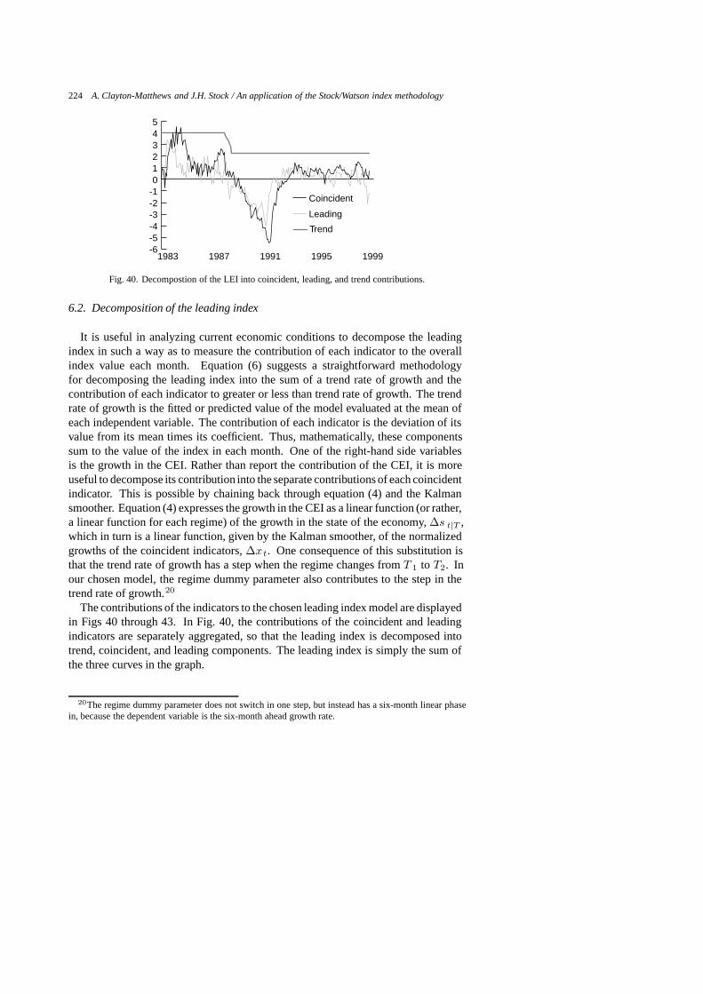
224 A. Clayton-Matthews and J.H. Stock / An application of the Stock/Watson index methodology
-6-5-4-3-2-1012345
Trend
Leading
Coincident
19991995199119871983
Fig. 40. Decompostion of the LEI into coincident, leading, and trend contributions.
6.2. Decomposition of the leading index
It is useful in analyzing current economic conditions to decompose the leadingindex in such a way as to measure the contribution of each indicator to the overallindex value each month. Equation (6) suggests a straightforward methodologyfor decomposing the leading index into the sum of a trend rate of growth and thecontribution of each indicator to greater or less than trend rate of growth. The trendrate of growth is the fitted or predicted value of the model evaluated at the mean ofeach independent variable. The contribution of each indicator is the deviation of itsvalue from its mean times its coefficient. Thus, mathematically, these componentssum to the value of the index in each month. One of the right-hand side variablesis the growth in the CEI. Rather than report the contribution of the CEI, it is moreuseful to decompose its contribution into the separate contributions of each coincidentindicator. This is possible by chaining back through equation (4) and the Kalmansmoother. Equation (4) expresses the growth in the CEI as a linear function (or rather,a linear function for each regime) of the growth in the state of the economy,∆s t|T ,which in turn is a linear function, given by the Kalman smoother, of the normalizedgrowths of the coincident indicators,∆xt. One consequence of this substitution isthat the trend rate of growth has a step when the regime changes fromT 1 to T2. Inour chosen model, the regime dummy parameter also contributes to the step in thetrend rate of growth.20
The contributions of the indicators to the chosen leading index model are displayedin Figs 40 through 43. In Fig. 40, the contributions of the coincident and leadingindicators are separately aggregated, so that the leading index is decomposed intotrend, coincident, and leading components. The leading index is simply the sum ofthe three curves in the graph.
20The regime dummy parameter does not switch in one step, but instead has a six-month linear phasein, because the dependent variable is the six-month ahead growth rate.
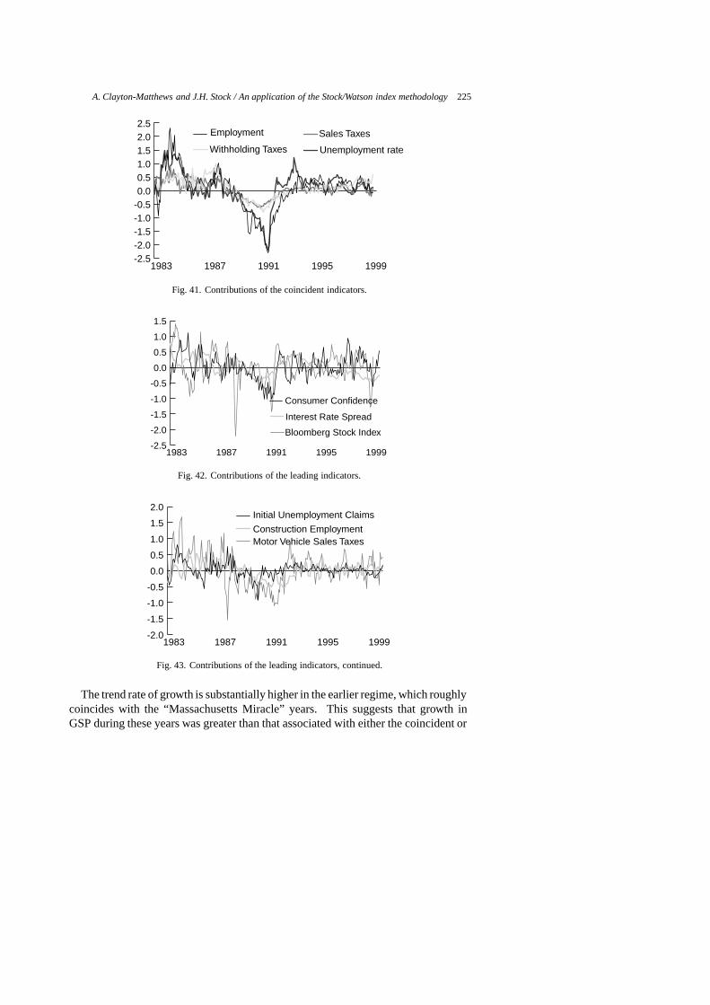
A. Clayton-Matthews and J.H. Stock / An application of the Stock/Watson index methodology 225
-2.5-2.0-1.5-1.0-0.50.00.51.01.52.02.5
Unemployment rate
Sales Taxes
Withholding Taxes
Employment
19991995199119871983
Fig. 41. Contributions of the coincident indicators.
-2.5
-2.0
-1.5
-1.0
-0.5
0.0
0.5
1.0
1.5
Bloomberg Stock Index
Interest Rate Spread
Consumer Confidence
19991995199119871983
Fig. 42. Contributions of the leading indicators.
-2.0
-1.5
-1.0
-0.5
0.0
0.5
1.0
1.5
2.0
Motor Vehicle Sales TaxesConstruction Employment
Initial Unemployment Claims
19991995199119871983
Fig. 43. Contributions of the leading indicators, continued.
The trend rate of growth is substantially higher in the earlier regime, which roughlycoincides with the “Massachusetts Miracle” years. This suggests that growth inGSP during these years was greater than that associated with either the coincident or
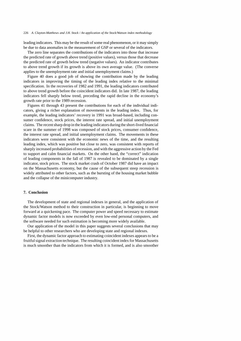
226 A. Clayton-Matthews and J.H. Stock / An application of the Stock/Watson index methodology
leading indicators. This may be the result of some real phenomenon, or it may simplybe due to data anomalies in the measurement of GSP or several of the indicators.
The zero line separates the contributions of the indicators into those that increasethe predicted rate of growth above trend (positive values), versus those that decreasethe predicted rate of growth below trend (negative values). An indicator contributesto above trend growth if its growth is above its own average value. (The converseapplies to the unemployment rate and initial unemployment claims.)
Figure 40 does a good job of showing the contribution made by the leadingindicators in improving the timing of the leading index relative to the minimalspecification. In the recoveries of 1982 and 1991, the leading indicators contributedto above trend growth before the coincident indicators did. In late 1987, the leadingindicators fell sharply below trend, preceding the rapid decline in the economy’sgrowth rate prior to the 1989 recession.
Figures 41 through 43 present the contributions for each of the individual indi-cators, giving a richer explanation of movements in the leading index. Thus, forexample, the leading indicators’ recovery in 1991 was broad-based, including con-sumer confidence, stock prices, the interest rate spread, and initial unemploymentclaims. The recent sharp drop in the leading indicators during the short-lived financialscare in the summer of 1998 was composed of stock prices, consumer confidence,the interest rate spread, and initial unemployment claims. The movements in theseindicators were consistent with the economic news of the time, and the resultingleading index, which was positive but close to zero, was consistent with reports ofsharply increased probabilities of recession, and with the aggressive action by the Fedto support and calm financial markets. On the other hand, the “correct” indicationof leading components in the fall of 1987 is revealed to be dominated by a singleindicator, stock prices. The stock market crash of October 1987 did have an impacton the Massachusetts economy, but the cause of the subsequent steep recession iswidely attributed to other factors, such as the bursting of the housing market bubbleand the collapse of the minicomputer industry.
7. Conclusion
The development of state and regional indexes in general, and the application ofthe Stock/Watson method to their construction in particular, is beginning to moveforward at a quickening pace. The computer power and speed necessary to estimatedynamic factor models is now exceeded by even low-end personal computers, andthe software needed for such estimation is becoming more widely available.
Our application of the model in this paper suggests several conclusions that maybe helpful to other researchers who are developing state and regional indexes.
First, the dynamic factor approach to estimating coincident indexes appears to be afruitful signal extraction technique. The resulting coincident index for Massachusettsis much smoother than the indicators from which it is formed, and is also smoother

A. Clayton-Matthews and J.H. Stock / An application of the Stock/Watson index methodology 227
than the index that would have resulted from the application of the BEA/ConferenceBoard composite index methodology. This smoothness characteristic is not uniqueto Massachusetts; similar results have been obtained for nearly every reported stateor regional index for which a Stock/Watson model has been estimated.
Second, the coincident index is in accord with our knowledge of the cyclical historyof the Massachusetts economy over the last quarter of the century. The index appearsto be capturing what it was intended to estimate.
Third, the leading index model appears to have a good chance of working satis-factorily. The leading indicators add predictive power over and above that providedby the CEI alone, and forecast reasonably well in sample. The relatively poor out ofsample forecast performancemay improve as informationaccumulates over time. Pa-rameter estimation and model selection can be periodically updated. Also, at least interms of in sample forecasts, the experience in other states where the Stock/Watsonmodel approach has been tried has been more successful overall. See Crone andBabyak [6], and Orr, Rich, and Rosen [12].
Fourth, pre-estimation filtering appears to be useful, especially because manystate and regional series are inherently noisy. A rational approach to pre-estimationfiltering may be a fruitful topic of future research. Transforming a set of indicatorsso that high-frequency noise is uniformly filtered out could make specification andestimation of index models easier. Such pre-filtering should be especially useful forthe more traditional BEA/Conference Board method, which averages only acrossindicators, not time.
Fifth, a systematic approach to model selection is probably a good thing. Ithas several advantages to a search over a limited number specifications where thepath to the final specification is determined by intuition and trial and error. Giventoday’s computing power, systematic approaches are practical. For example, ourspecification search for the leading index model entailed running over two millionregressions, yet involved only a few hours of computer time on a relatively slowprocessor. Nevertheless, model selection is still subjective, especially when thehistorical record is short as in Massachusetts, which limits the power of techniquessuch as PLS.
Last, a probability of recession index would be a useful addition to the leadingindex. It would help the analyst quantify the likelihood of a turning point occurrencewhen the signal is ambiguous, e.g., when the index changes sign temporarily, orforecasts near zero growth. Several alternatives are available, including Stock andWatson [16,17], Phillips [13], and Orr, Rich, and Rosen [12].
Appendix A. De-normalization of the Kalman state: A comparison with theBEA/TCB methodology
The state that is output from the Kalman filter in the model given in equations (1)–(3) is, by construction, normalized to be driftless, with unit-variance input shocks.
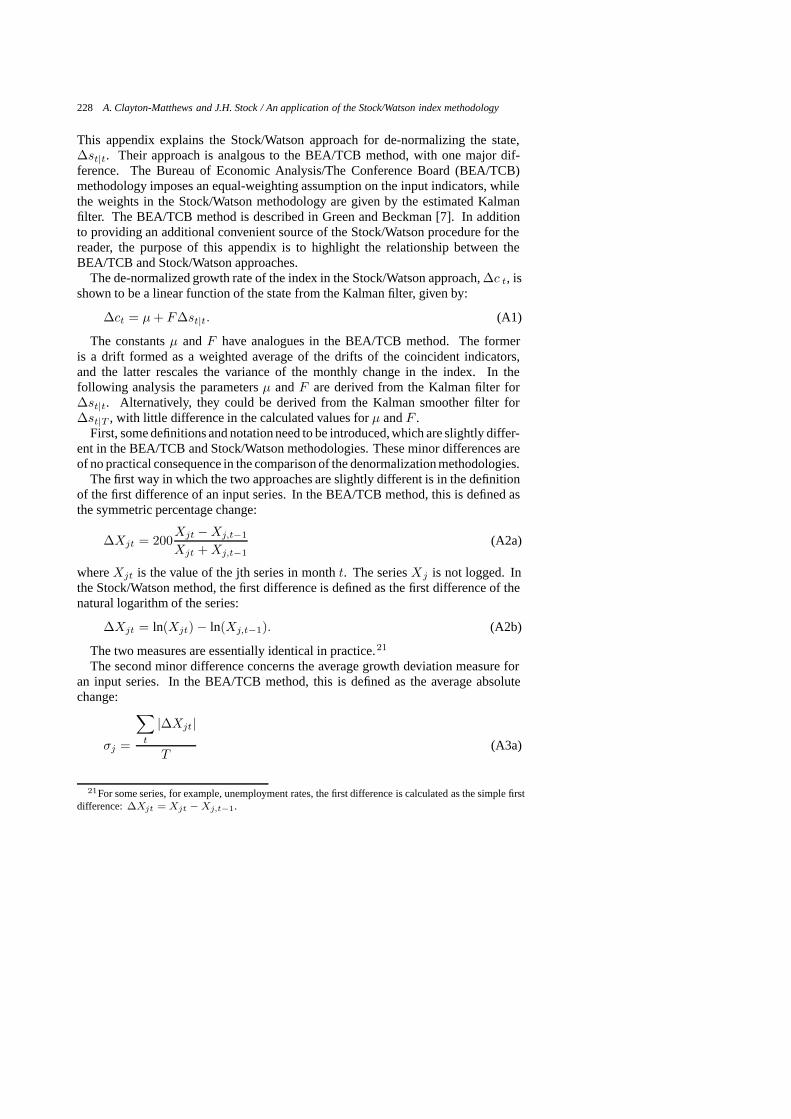
228 A. Clayton-Matthews and J.H. Stock / An application of the Stock/Watson index methodology
This appendix explains the Stock/Watson approach for de-normalizing the state,∆st|t. Their approach is analgous to the BEA/TCB method, with one major dif-ference. The Bureau of Economic Analysis/The Conference Board (BEA/TCB)methodology imposes an equal-weighting assumption on the input indicators, whilethe weights in the Stock/Watson methodology are given by the estimated Kalmanfilter. The BEA/TCB method is described in Green and Beckman [7]. In additionto providing an additional convenient source of the Stock/Watson procedure for thereader, the purpose of this appendix is to highlight the relationship between theBEA/TCB and Stock/Watson approaches.
The de-normalized growth rate of the index in the Stock/Watson approach,∆c t, isshown to be a linear function of the state from the Kalman filter, given by:
∆ct = µ + F∆st|t. (A1)
The constantsµ andF have analogues in the BEA/TCB method. The formeris a drift formed as a weighted average of the drifts of the coincident indicators,and the latter rescales the variance of the monthly change in the index. In thefollowing analysis the parametersµ andF are derived from the Kalman filter for∆st|t. Alternatively, they could be derived from the Kalman smoother filter for∆st|T , with little difference in the calculated values forµ andF .
First, some definitions and notation need to be introduced, which are slightly differ-ent in the BEA/TCB and Stock/Watson methodologies. These minor differences areof no practical consequence in the comparison of the denormalization methodologies.
The first way in which the two approaches are slightly different is in the definitionof the first difference of an input series. In the BEA/TCB method, this is defined asthe symmetric percentage change:
∆Xjt = 200Xjt − Xj,t−1
Xjt + Xj,t−1(A2a)
whereXjt is the value of the jth series in montht. The seriesXj is not logged. Inthe Stock/Watson method, the first difference is defined as the first difference of thenatural logarithm of the series:
∆Xjt = ln(Xjt) − ln(Xj,t−1). (A2b)
The two measures are essentially identical in practice.21
The second minor difference concerns the average growth deviation measure foran input series. In the BEA/TCB method, this is defined as the average absolutechange:
σj =
∑t
|∆Xjt|
T(A3a)
21For some series, for example, unemployment rates, the first difference is calculated as the simple firstdifference:∆Xjt = Xjt − Xj,t−1.
A. Clayton-Matthews and J.H. Stock / An application of the Stock/Watson index methodology 229
whereT is the number of observations for the series. In the Stock/Watson method,the measure is the standard deviation:
σj =
√√√√√∑
t
(∆Xjt − µj)2
T − 1(A3b)
where the mean of the series,µj , is defined the same in both approaches:
µj =
∑t
∆Xjt
T. (A4)
The difference in the deviation measures imparts a very minor difference in thecalculated weights between the two approaches that would otherwise not be present.
We will need to use the standardized first difference of an input series, defined as:
∆xjt =∆Xjt − µj
σj(A5)
The main difference between the two approaches is the manner in which the inputseries are filtered to produce the estimated state of the economy. In the Stock/Watsonapproach, the state is calculated according to:
∆st|t =∑
j
mj(L)∆xjt, (A6)
where
mj(L) = mj0L0 + mj1L
1 + mj2L2 + · · · (A7a)
is the Kalman filter.22 In factor analysis terminology, the filter would be called the“scoring coefficients”, since they transform observations on several variables (forexample, answers to a battery of questions) into a factor score (for example, anintelligence or attitude index). Stock and Watson call the filter the set of dynamicmultipliers, which reflects the way the filter is calculated in practice, i.e., by observinghow the series∆sk|k, k � t, changes in response to a one-time unit change in∆x jt
(a pulse equal to one in periodt and zero before and after periodt).In the BEA/TCB methodology, the Kalman filter is effectively replaced by the
following:
mj(L) = m. (A7b)
22L is the lag operator, i.e.,Lk∆xt = ∆xt−k.
230 A. Clayton-Matthews and J.H. Stock / An application of the Stock/Watson index methodology
This is the essence of the “equal weighting” methodology. Each normalized seriesenters the index equally. It doesn’t matter what the value ofm is, so the BEA/TCBmethod implicitly usesm = 1. Furthermore, the composite is formed only from thecontemporaneous values of the indicators.
We now show how the BEA/TCB de-normalized index is formed. This closelyfollows the procedure given in Green and Beckman [7], with slight differences innotation needed to highlight the relationship with the Stock/Watson method. First,define
Bj =mj(1)
σj, where, from (A7a), mj(1) =
∑k�0
mjk. (A8a)
Note that, from (A7b), this simplifies to
Bj =m
σj(A8b)
for the BEA/TCB methodology. Next, define
F =1∑
j
Bj
, and (A9)
wj = FBj . (A10)
Note that∑
j
wj = 1. Also define a weighted mean growth rate:
µ =∑
j
wjµj . (A11)
In the BEA/TCB methodology, the growth of the denormalized index can now beexpressed as:
∆ct = µ +∑
j
Wj(∆Xjt − µj) =∑
j
wj∆Xjt. (A12)
We now show how this is equivalent to (A1), when one substitutes the Kalman filterfor the equal weighting scheme of the BEA/TCB. Begin by using (A5) to replace∆Xjt in the middle portion of (A12) byσj∆xjt + µj .
∆ct = µ +∑
j
wjσj∆xjt. (A13)
Using (A10), this becomes
∆ct = µ + F∑
j
Bjσj∆xjt. (A14)
A. Clayton-Matthews and J.H. Stock / An application of the Stock/Watson index methodology 231
Using (A8b), this simplifies to
∆ct = µ + F∑
j
m∆xjt. (A15)
Now the crucial substitution of the Kalman filter is made, using (A7b):
∆ct = µ + F∑
j
mj(L)∆xjt. (A16)
Finally, substituting (A6) for the summation gives us (A1):
∆ct = µ + F∆st|t. (A17)
So the denormalized growth in the index in the Stock/Watson methodology is a lin-ear function of the state from the state space model in equations (1)–(3). Furthermore,the only essential difference between the Stock/Watson and BEA/TCB methodologiesis the use of the Kalman filter in place of the equal weighting assumption.
Appendix B. Calibrating the Kalman state to Gross State Product
This appendix describes how the state vector from the model in equations (1)–(3)was calibrated to Massachusetts Gross State Product, i.e., it describes how the coef-ficientsa1, b1, a2, andb2 in equation (4) were calculated. The procedure describedbelow can be used to fit the index to the first two moments of the growth – the averagegrowth rate and average deviation from trend – of any observable series.
Consider an index constructed from the state output by the Kalman filter so thatits growth is a linear function of the state:
∆c′t = µ + F∆st|T . (B1)
The construction of such an index is described in Appendix A, but this appendixis also applicable to calibrating the state vector directly, i.e., whenµ = 0 andF = 1.∆c′t represents the growth in the index, or the first difference of the log of the index.Suppose that the calibration is to be performed to fit Gross State Product over theperiod of timet ∈ T . This appendix describes how to choose the parametersa andbso that the linear function of the state
∆ct = a + b∆st|T (B2)
matches the first two moments of Gross State Product growth during the periodT .Suppose that the first two moments of∆c′t from (B1) aregc anddc respectively,
i.e., they are respectively, the mean and standard deviation of∆c ′t over the period
232 A. Clayton-Matthews and J.H. Stock / An application of the Stock/Watson index methodology
T.23 Suppose also that the first two moments of the growth of Gross State Productover the periodT aregGSP anddGSP respectively.24
The desired parameters in (B2) can be derived in two simple steps. First, detrendand standardize (B1) over the periodT by subtracting its growth and dividing by theaverage deviation:
∆c′′t =µ + F∆st|T − gc
dc. (B3)
Next, reconstitute∆c′′t so that is has an average growth ofgGSP and an averagedeviation ofdGSP :
∆ct = ∆c′′t dGSP + gGSP = fF∆st|T + f(µ − gc) + gGSP ,(B4)
wheref =dGSP
dc.
Then
a = f(µ − gc) + gGSP
b = fF. (B5)
In order to get a satisfactory fit, it may be necessary to apply this procedurepiecewise by dividing the entire span of the index and Gross State Product into twoor more periods. For our index, two periods, 1978–1987 and 1988–1996, weredeemed to be satisfactory.
Acknowledgements
We gratefully acknowledge helpful comments from Robert Rich and an anonymousreferee. We also thank Douglas Woodward and Charles Renfro for their support andpatience throughout the project, as well as the University of Minho, Braga, Portugaland their faculty and staff for hosting the Workshop on Regional Economic IndicatorModels, at which an earlier version of this paper was presented. This research wassupported by a Public Service Grant from the University of Massachusetts Boston.Software for estimating the coincident index model is available from Alan Clayton-Matthews ([email protected]), who is also responsible for remaining errors andomissions.
23We used the average absolute deviation, but the same procedure would apply to the standard deviation.Also, because the index is monthly but Gross State Product is annual,∆c′t was annualized beforecalculating the moments. The growth rategc was expressed as a monthly growth rate in order to beconsistent withµ from (B1). The average deviation,dc , was retained in annual units.
24The growth rategGSP is expressed as a monthly growth rate, in order to be consistent withgc andµ.
A. Clayton-Matthews and J.H. Stock / An application of the Stock/Watson index methodology 233
References
[1] B.D.O. Anderson and J.B. Moore,Optimal Filtering, Prentice Hall, Englewood Cliffs, New Jersey,1979.
[2] A. Clayton-Matthews, DSFM manual: version 2/23/99, mimeo, 1999.[3] A. Clayton-Matthews, Y.K. Kodrzycki and D. Swaine, Indexes of economic indicators: what can
they tell us about the New England economy,New England Economic Review (November/December1994), Federal Reserve Bank of Boston, 17–41.
[4] T.M. Crone, New indexes track the state of the states,Business Review (January/February 1994),Federal Reserve Bank of Philadelphia, 19–31.
[5] T.M. Crone, Using state indexes to define economic regions in the US, paper prepared for theWorkshop on Regional Economic Indicator Models, Braga, Portugal, June 8–10, 1998.
[6] T.M. Crone and K.J. Babyak, Looking ahead: leading indexes for Pennsylvania and New Jersey,Business Review (May/June 1996), Federal Reserve Bank of Philadelphia, 3–14.
[7] G.R. Green and B.A. Beckman, Business cycle indicators: upcoming revision of the compositeindexes,Survey of Current Business (October 1993), 44–51.
[8] J.D. Hamilton,Time Series Analysis, Princeton University Press, Princeton, New Jersey, 1994.[9] R.W. Hamming,Digital Filters, (Third ed.), Dover Publications, Mineola, New York, 1998.
[10] W.K. Newey and K.D. West, A simple, positive semi-definite, heteroskedasticity and autocorrelationconsistent covariance matrix,Econometrica 55(3) (May 1987), 703–708.
[11] J. Orr, R. Rich and R. Rosen, Two new indexes offer a broad view of economic activity in the NewYork – New Jersey region,Current Issues in Economics and Finance 5(14) (October 1999), FederalReserve Bank of New York.
[12] J. Orr, R. Rich and R. Rosen, Leading economic indicators for New York and New Jersey, mimeo,Federal Reserve Bank of New York, September 30, 1999.
[13] K.R. Phillips, The Texas index of leading economic indicators: a revision and further evaluation,Economic Review (July 1990), Federal Reserve Bank of Dallas.
[14] T.J. Sargent and C.A. Sims, Business cycle modeling without pretending to have too much a priorieconomic theory, in:New Methods in Business Cycle Research: Proceedings from a Conference,Federal Reserve Bank of Minneapolis, 1977.
[15] J.H. Stock and M.W. Watson, New indexes of coincident and leading economic indicators,NBERMacroeconomics Annual (1989), 351–394.
[16] J.H. Stock and M.W. Watson, A probability model of the coincident economic indicators, in:Leading Economic Indicators: New Approaches and Forecasting Records, K. Lahiri and G.H.Moore, eds., Cambridge University Press, Cambridge, 1991, pp. 63–89.
[17] J.H. Stock and M.W. Watson, A procedure for predicting recessions with leading indicators: econo-metric issues and recent experience, in:Business Cycles, Indicators, and Forecasting, J.H. Stockand M.W. Watson, eds., The University of Chicago Press, Chicago and London, 1993, pp. 95–156.
[18] C.K.H. Tsao, The Massachusetts stock index: methodology in construction using historical data,mimeo, University of Massachusetts Boston, 1998.
[19] C.K.H. Tsao, Regional coincident economic indexes: an investigation of the New England states’“state of the economy”, Ph.D. Dissertation, University of Massachusetts Boston, 1999.
[20] C.Z. Wei, On predictive least squares principles,The Annals of Statistics 20(1) (1992), 1–42.