66 TRANSPORTATION RESEARCH RECORD 1251

An Application of Optimal Control Theory to Dynamic User Equilibrium Traffic Assignment

BYUNG-WooK Wrn

Optimal control theory is applied to the problem of dynamic traffic assignment, corresponding to user optimization, in a congested network with one origin-destination pair connected by N parallel arcs. Two continuous time formulations are considered, one with fixed demand and the other with elastic demand. Optimality con­ditions are derived by Pontryagin's maximum principle and inter­preted as a dynamic generalization of Wardrop's first principle. The existence of singular controls is examined, and the optimality of singular controls is assured by the generalized convexity con­ditions. Under the steady-state assumptions, a dynamic model with elastic demand is shown to be a proper extension of Beckmann's equivalent optimization problem with elastic demand. Finally, the derivation of the dynamic user optimization objective functional is demonstrated, which is analogous to the derivation of the objec­tive function of Beckmann's mathematical programming formu­lation for user equilibrium.

The objective of this paper is to explore the application of optimal control theory to the problem of dynamic traffic assignment corresponding to user optimization. Two contin­uous time optimal control problems will be formulated, one with fixed demand and the other with elastic demand. The present paper is concerned with dynamic extensions of the steady-state network equilibrium model, particularly Beck­mann's equivalent optimization problem, which is a mathe­matical programming formulation (1). This formulation is based on the steady-state assumptions:

(1). The average arc travel cost is some known function of the total traffic flow traversed during the period of analysis;

(2). Travel demands associated with each origin-destination (0-D) pair are constant over time; and

(3). Flow entering each arc is always equal to flow leaving that arc during the period of analysis.

Hence, the relaxation of the steady-state assumptions lead to the problem of dynamic traffic assignment in which the net­work characteristics are explicit functions of time.

A pioneering research in dynamic traffic assignment was accomplished by Merchant and Nemhauser (2-4). They for­mulated the model as a discrete time, nonlinear, and non­convex mathematical program corresponding to system optimization in a multiple-origin single-destination network. They showed that the Kuhn-Tucker optimality conditions can be interpreted as a generalization of Wardrop's second prin-

Department of City and Regional Planning, University of Pennsyl­vani3, Philadelphia 19104.

ciple, which requires equalization of certain marginal travel costs for all the paths that are being used. The behavior of their dynamic model was also examined under the steady­state assumptions, and as a result the model was proven to be a proper generalization of the conventional static system optimal traffic assignment model.

The algorithmic question of implementing the Merchant­Nemhauser (M-N) model was resolved by Ho (5). He showed that, for a piecewise linear version of the M-N model, a global optimum is contained in the set of optimal solutions of a certain linear program. He also presented a sufficient con­dition for optimality, which implies that a global optimum can be obtained by successively optimizing at most N + 1 objective functions for the linear program, where N is the number of time periods in the planning horizon.

Recently Carey (6) resolved a hitherto open question as to whether the M-N model satisfies a constraint qualification. It was shown that the M-N model does in fact satisfy a constraint qualification, which establishes the validity of the optimality analysis presented by Merchant and Nemhauser (4). More recently, Carey (7) reformulated the M-N model as a convex nonlinear mathematical program. As a consequence, the new formulation could have analytical, computational, and inter­pretational advantages in comparison with the original M-N model. In particular, the Kuhn-Tucker conditions are both necessary and sufficient to characterize an optimal solution; in the M-N model, however, they are not sufficient because the constraint set is not convex.

In contrast with the atoremenuoned mathematical pro­gramming approaches, Luque and Friesz (8) provided a new insight into the problem of dynamic traffic assignment through the application of optimal control theory. They formulated the M-N model as a continuous time-optimal control problem corresponding to system optimization. The optimality conditions were derived by applying Pontryagin's maximum principle, and economic interpretation was conducted and compared with those obtained from Merchant and Nemhauser (4).

It is worth noting that the Merchant-Nemhauser model and its extended models consider a system-optimized flow pattern that satisfies a dynamic generalization of Wardrop's second principle. In general, a traffic flow pattern obeying Wardrop's second principle minimizes the total transportation cost of the network as a whole, and it can be regarded as the most desir­able flow pattern for society. In the present paper, however, we are interested in a user-optimized flow pattern obeying a dynamic generalization of Wardrop's first principle, which

Wie

requires equalization of certain unit travel costs for all the paths that are being used . Suppose that travel demands are time-dependent but fixed in a multiple 0-D network. The problem of dynamic traffic assignment corresponding to user optimization can be viewed as a noncooperative game between players associated with various 0-D pairs and departure times. Wardrop's first principle can then be generalized for dynamic traffic assignment such that:

Individual drivers attempt to minimize their own travel costs by changing routes. At each instant in time , no one can reduce his or her travel costs by unilaterally changing routes; there­fore , the unit travel costs on paths used by drivers who have the same departure time and 0-D pair are identical and equal to the minimum unit path costs for that 0-D pair.

Our analysis is restricted to the network with one 0-D pair that is connected by N parallel arcs, as shown in. Figure 1. It is also assumed that there is one transport mode-for exam­ple , private automobile. Note that A is the set of directed arcs. We will use index a to denote a directed arc. We will consider a fixed planning horizon of length T; that is, all activities occur at some time t E [O, T]. In the remainder of this paper, traffic flow is defined as the average number of vehicles passing a fixed point of an arc per unit of time, and traffic volume is defined as the total number of vehicles accu­mulated on arc a at some time t E [O , T] .

Our dynamic model is related to models proposed by Hur­dle (9), Hendrickson and Kocur (10), Mahmassani and Her­man (11), Mahmassani and Chang (12), de Palma et al. (13), Ben-Akiva et al. (14,15) , Smith (16) , Daganzo (17), and New­ell (18). But our model differs in important aspects, which include its formulation as a continuous time optimal control problem. We do not attempt to compare our model with models proposed by the authors just cited . One may refer to Friesz (19) and Alfa (20) for literature reviews on the dynamic network equilibrium models proposed to date.

ASSUMPTIONS

Exit Function

The flow leaving arc a E A is a function of the traffic volume accumulated on that arc at time t E (0 , T]. The exit functions g.(x.(t)] are concave, differentiable, nondecreasing, and non­negative for all x.(t) ;::: 0, with the additional restriction that g.(O) = 0 (Figure 2).

Origin

N

67

Demand Function

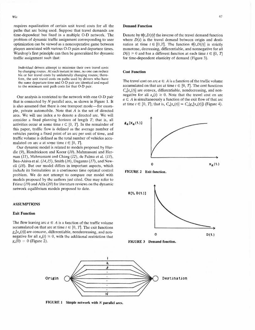
Denote by 0(t,D(t)] the inverse of the travel demand function where D(t) is the travel demand between origin and desti­nation at time t E (O,T]. The function 0[t,D(t)] is strictly monotone, decreasing, differentiable, and nonnegative for all D(t) ;::: 0 and has a different function at each time t E (0, T] for time-dependent elasticity of demand (Figure 3).

Cost Function

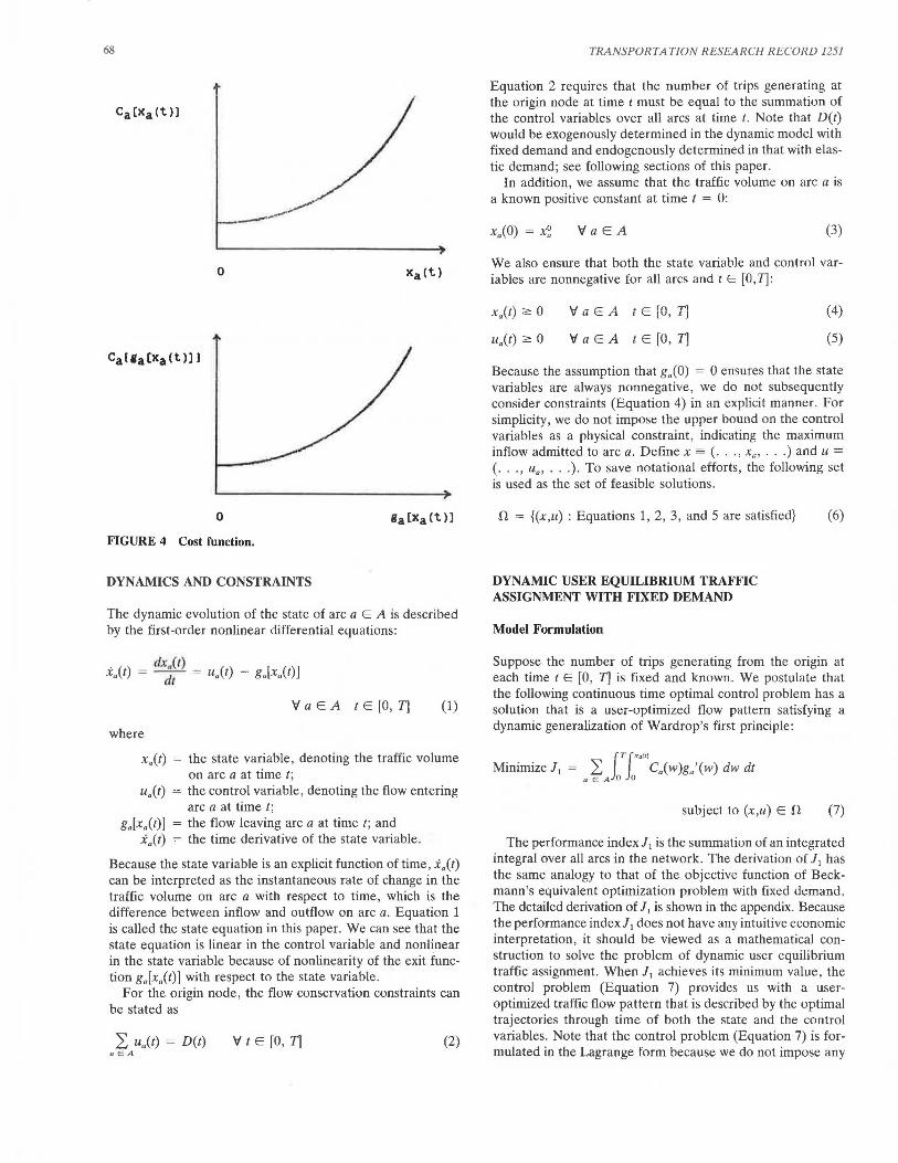
The travel cost on arc a E A is a function of the traffic volume accumulated on that arc at time t E [O, T]. The cost functions c.(x.(t)] are convex, differentiable , nondecreasing, and non­negative for all x.(t) ;::: 0. Note that the travel cost on arc a E A is simultaneously a function of the exit flow of that arc at time t E (0, T]; that is, C.(x.(t)) == C.{g.[x.(t)]} (Figure 4).

0

FIGURE 2 Exit function.

0[t,D(t))

0 D(t)

FIGURE 3 Demand function.

Destination

FIGURE 1 Simple network with N parallel arcs.

68

0

0

FIGURE 4 Cost function.

DYNAMICS AND CONSTRAINTS

The dynamic evolution of the state of arc a E A is described by the first-order nonlinear differential equations:

. dx,,(i) xa(t) = --;ft = ua(t) - g.[x.(t)]

\;/ a E A t E [O, 71 (1)

where

x.(t) = the state variable, denoting the traffic volume on arc a at time t;

u.(t) = the control variable, denoting the flow entering arc a at time t;

g.[x.(t)] = the flow leaving arc a at time t; and x.(t) = the time derivative of the state variable.

Because the state variable is an explicit function of time, x.(t) can be interpreted as the instantaneous rate of change in the traffic volume on arc a with respect to time, which is the difference between inflow and outflow on arc a. Equation 1 is called the state equation in this paper. We can see that the state equation is linear in the control variable and nonlinear in the state variable because of nonlinearity of the exit func­tion g.[x.(t)] with respect to the state variable.

For the origin node, the flow conservation constraints can be stated as

L u.(t) = D(t) \;/ t E [O, 71 (2) a EA

TRANSPORTATION RESEARCH RECORD 1251

Equation 2 requires that the number of trips generating at the origin node at time t must be equal to the summation of the control variables over all arcs at time t. Note that D(t) would be exogenously determined in the dynamic model with fixed demand and endogenously determined in that with elas­tic demand; see following sections of this paper.

In addition, we assume that the traffic volume on arc a is a known positive constant at time t = 0:

x.(O) = x~ Va EA (3)

We also ensure that both the state variable and control var­iables are nonnegative for all arcs and t E [O, T]:

x.(t) ::=::: 0

u.(t) ~ 0

V a E A t E [0, TJ

V a E A t E [0, 71

(4)

(5)

Because the assumption that g.(O) = 0 ensures that the state variables are always nonnegative, we do not subsequently consider constraints (Equation 4) in an explicit manner. For simplicity, we do not impose the upper bound on the control variables as a physical constraint, indicating the maximum inflow admitted to arc a. Define x = ( .. ., x., . .. ) and u = ( .. ., u., ... ). To save notational efforts, the following set is used as the set of feasible solutions.

D = {(x,u) : Equations 1, 2, 3, and 5 are satisfied}

DYNAMIC USER EQUILIBRIUM TRAFFIC ASSIGNMENT WITH FIXED DEMAND

Model Formulation

(6)

Suppose the number of trips generating from the origin at each time t E [O, 71 is fixed and known. We postulate that the following continuous time optimal control problem has a solution that is a user-optimized flow pattern satisfying a dynamic generalization of Wardrop's first principle:

Minimize 11

= L lTlx.ii>C.(w)ga'(w) dw dt a EA 0 0

subject to (x,u) E D (7)

The performance index 11 is the summation of an integrated integral over all arcs in the network. The derivation of 11 has the same analogy to that of the objective function of Beck­mann's equivalent optimization problem with fixed demand. The detailed derivation of 1, is shown in the appendix. Because the performance index 11 does not have any intuitive economic interpretation, it should be viewed as a mathematical con­struction to solve the problem of dynamic user equilibrium traffic assignment. When 11 achieves its minimum value, the control problem (Equation 7) provides us with a user­optimized traffic flow pattern that is described by the optimal trajectories through time of both the state and the control variables. Note that the control problem (Equation 7) is for­mulated in the Lagrange form because we do not impose any

Wie

state constraint at the terminal time T. We shall suppress the time notation (t) when no confusion arises.

Optimality Conditions

The necessary conditions for an optimal solution of the control problem (Equation 7) can be derived by Pontryagin's maxi­mum principle [Pontryagin et al., (21)]. As a first step in analyzing the necessary conditions, we construct the Hamil­tonian:

H = L {xaCa(w)ga'(w)dw + L 'Ya·[ua - ga(xa)] aEAJo aEA

+ µ-[D - L ual + L f3a"[ -ual (8) aEA a EA

where 'Ya(t) is the costate variable associated with the ath state Equation 1; µ(t) is the Lagrange multiplier associated with the flow conservation constraints at the origin; and f3a(t) is also the Lagrange multiplier associated with nonnegativity of the ath control variable.

We can obtain the first-order necessary conditions, also known as the Euler-Lagrange equations in the calculus of variations. The differential equations governing the evolution of the costate variables 'Ya are given from the Hamiltonian (Equation 8), which require [see Bryson and Ho, (22)]:

aH

= [C.(xa) 'Ya] g a' (xa) \>'aEA tE[O,T] (9)

Equation 9 will be called the costate equation. Boundary conditions on the costate variables are obtained by the trans­versality conditions:

'Ya(T) = Q \>'a EA (10)

According to Pontryagin's maximum principle, the Ham­iltonian must be minimized at each time t E [O, T]. The Kuhn­Tucker optimality conditions for u! to be an optimal solution that minimizes the Hamiltonian are readily obtained as:

aH Q = 'Ya - µ - f3a \>'a EA (11)

f3a 2'.: 0 and f3a . ua = 0 'v' a EA (12)

In the terminology of optimal control theory, aH/aua is often called impulse response function because the gradient of the Hamiltonian with respect to the control variable represents the variation in the performance index 11 as a consequence of a unit impulse in the corresponding control variable at time t, while holding x~ constant and satisfying the state equation (Equation 1). In particular, Equation 12 contains the com­plementary slackness conditions to take into account non­negativity of the control variables.

The preceding necessary conditions for optimality may be collected in the following compact form:

-'Ya = [ C.(xa) - 'Ya] g~(xa) \>'a EA tE[O, T] (13)

'Ya(T) = 0 \>'a EA

\>'a EA tE [O, T]

\>'aEA tE[O,T]

69

(14)

(15)

(16)

The optimality conditions (Equations 13-16) can be under­stood such that if at some time t E [O, T] 'Ya > µ for all a E A, the flow entering arc a is equal to zero, and if 'Ya = µ, ua is either zero or singular in nature. Singular ·control is dis­cussed further in the next section. It is implied that the quan­tities determining the control variable ua are the value of ['Y~ - µ],which is the difference between the costate variable and the Lagrange multiplier. Hence, we may conjecture that the optimality conditions are analogous to the principle of the flow of electricity, in which electric current moves from a node with higher voltage to a node with lower voltage.

The Arrow-Kurz sufficiency theorem (23, 24) ensures that the necessary conditions are also sufficient when the Hamil­tonian is convex in the state variables. We can see that the Hamiltonian (Equation 8) is convex in the state variables under the assumptions made previously. Hence, the opti­mality conditions (Equations 13-16) are necessary and also sufficient.

Singular Controls

Because the Hamiltonian (Equation 8) is linear in the control variable, the gradient of the Hamiltonian with respect to ua does not depend on the control variable. Therefore, the opti­mality conditions for u: to be an optimal control that min­imizes the Hamiltonian provide no useful information to determine the optimal control in terms of the state and costate variables. In this case we must take successive time derivatives

aH of - = 'Y - µ - f3a and make appropriate substitutions

aua a

by using the state Equation 1 and the costate Equation 9 until we find an explicit expression for the control variables. The optimal control determined by this procedure is called a sin­gular control. A finite time interval for which a singular con­trol exist is called a singular interval. An extremal arc on

which the determinant of the matrix ji_ [aH] vanishes iden-iJ 110 dll0

tically is called a singular arc. To determine the singular control, we must use the fact

that successive time derivatives of the gradient of the Ham­iltonian would be also constant and equal to zero on a singular arc. The first and second time derivatives of the gradient of the Hamiltonian with respect to ua give the following relationship:

'Ya= fl and :Ya= fl (17)

We substitute the costate equation (Equation 9) into the first relationship in Equation 17:

(Ca - 'Ya)g~ + Jl = Q (18)

The second time derivatives of Equation 18 are calculated:

(C:,Xa - 'Ya)g~ + (Ca - 'Ya)g~ Xa + J1 = Q (19)

70

By using the state equation (1), we may manipulate Equation 19 to yield the following expression for the smgular control:

µg,: - j.i. + (C~g~ + (C. - µ)g:Jgrt I I + c ) II ,.ga " - µ g.

(20)

One may ask whether the singular control given by Equa­tion 20 is optimal or not. To answer this question, we shall derive the necessary conditions for optimality of singular con­trols. The generalized convexity condition can be obtained elsewhere (22):

a [ d2 [aHJJ

aua dt 2 aua -(Ca - 'Ya)g~ - Cg~:::; 0

(21)

According to the costate equations (Equation 9) and assump­tions made earlier, the generalized convexity conditions are satisfied. Hence, we can conclude that the singular control (Equation 20) is optimal.

Dynamic User Equilibrium Principle

The important question now arises as to whether or not a traffic flow pattern, described by time trajectories of the state and control variables as an optimal solution of Equation 7, satisfies a dynamic generalization of Wardrop's first principle. To answer this question, we define the following function by manipulating the costate equation (Equation 9):

<l>a(t) = C.(xa) + 'Y)g~(xa) \faEA tE[O,T] (22)

It is well known that when the performance index 11 achieves its minimum value l~, we have the following properties (22):

ar 'Ya(t) =_I_

c1x.,(t)

. d ( iJ}I ) 'Y.(t) = dt 1Jx,,(1) \f a E A t E [O, T] (23)

We see that 'Y.(t) is the time rate of change in the value of the performance index 11 as a consequence of a change in the corresponding state variable x0 (t) along the optimal state tra­jectory at time t E [O, T]. Therefore, we may interpret <l>a(t) as the sum of static and dynamic terms: C.(x.) is the unit travel cost on arc a that is equilibrated in the static user optimization problem; and 'Y.I g~ is· regarded as the contri­bution to arc unit travel cost due to the dynamic nature of our control problem. In the present paper, we call <l>.(t) the instantaneous travel cost on arc a EA at time t E [O, T].

We are now ready to state and prove the following theorem:

Theorem 1: If at some time t E [O, T], u. > 0 for all a EA, then <l>0 (t) = inf {<l>"(t) : \fa EA}.

TRANSPORTATION RESEARCH RECORD 1251

Proof. From the costate equation (9), we see that

\f a E A t E [O, T] (24)

However, from Equation 15, we know that

'Ya 2" µ \f a E A t E [O, T] (25)

It follows at once from Equations 24 and 25 that

<l>.(t) 2" µ \f a E A, t E [0, T] (26)

\l./e also know that if ua > 0 for all a c:: A, then Equation 25 holds as an equality because of the complementary slackness conditions of Equations 15 and 16. Hence, the theorem is immediately proved.

Theorem 1 tell us that user equilibrium conditions hold at each instant in our dynamic model. Hence, we regard Theo­rem 1 as a dynamic generalization of Wardrop's first principle, which is termed the Dynamic User Equilibrium Principle in the present paper. But it is restricted to a network with one 0-D pair connected by N parallel arcs. This principle can also be restated at each instant t E [O, T]:

u.(t) > 0

u0 (t) = 0

fora= 1,2,. .. . ,k

for a = k + 1, ... ., N

DYNAMIC USER EQUILIBRIUM TRAFFIC ASSIGNMENT WITH ELASTIC DEMAND

Model Formulation

(27)

(28)

(29)

Suppose that travel demands change in response to travel costs between the elements of an origin-destination pair. We pos­tulate that the following continuous, time-optimal control problem has a solution that is a user-optimized flow pattern obeying a dynamic generalization of Wardrop's first principle:

Minimize 12 = L {T rx·(•) c.(w)g~(w) dw dt a E A Jo Jo

{T (D(t)

- Jo Jo 0(t, y) dy dt

subject to

(x, u) E !1

D(t) = L u.(t) a EA

(30)

where D(t) is the number of trips generating at the origin at time t E [O, T] and 0[t, D(t)] is the inverse of the travel demand function. Note that D(t) is determined endogenously in the control problem (Equation 30). The performance index 12 is decomposed into two terms: the performance index 11 and an integrated integral of the inverse demand function.

Wie

Optimality Conditions

To analyze the necessary conditions, we construct the Ham­iltonian:

ix, iD H = L Ca(w)g;(w) dw - 6(t, y) dy

aEA 0 0

+ L 'Ya · [u. - ga(x.)] + L ~a · [ -u.] (31) a EA a E A

It is important to note that the second term of H is strictly concave in the control variable ua because the integral of a monotone decreasing function is strictly concave. The nega­tive of a strictly concave function is, however, a strictly convex function.

The costate equations and transversality conditions are identical to Equations 9 and 10, respectively. The Kuhn-Tucker optimality conditions for the minimization of the Hamiltonian (Equation 31) with respect to the control variables are obtained:

aH - = 0 = 'Ya - 6[t, L Ua] - ~a aua aEA

'v'a EA (32)

~. 2: 0 and ~. · Ua = 0 'v'a EA (33)

We may collect the necessary conditions for optimality of the problem of dynamic user equilibrium traffic assignment with elastic demand in the following compact form:

-'Ya= [C.(xa) - 'Ya]g;(xa)

-y0 (T) = 0

'Ya - 62:0

Ua ·('Ya - 6) = 0

'v'aEA tE[O,T]

'v'aEA

'v'aEA tE[O, T]

'v'aEA tE[O,T]

(34)

(35)

(36)

(37)

It can be understood from the optimality conditions (Equa­tions 34-37) that if at some time t E [O, T] 'Ya > 6 for all a E A, the flow entering arc a is equal to zero; and if 'Ya = 6, then ua is explicitly determined by the state equation (Equa­tion 1) and the costate equation (9) as a solution of a two­point boundary-value problem. It is worth noting that the control problem (Equation 30) does not have singular controls.

The Arrow-Kurz sufficiency theorem (23, 24) ensures that the optimality conditions (Equations 34-37) are necessary and also sufficient, because the Hamiltonian (Equation 31) is convex in the state variables under the assumptions made previously. In addition, Theorem 1 holds for the dynamic model (Equation 30) except for the fact that µ(t) is replaced by 6[t, D(t)] in Equations 25 and 26.

Equivalency Under the Steady-State Assumptions

We wish to assure that the control problem (Equation 30) is a proper dynamic extension of Beckmann's equivalent optimi­zation problem with elastic demand. To do this, we examine the behavior of our dynamic model under the steady-state assumptions, such that the time rate of a change in the traffic

71

volume on each arc would be zero during [O, T] and travel demands would be constant over time.

Through a change of the variables of integration, we may rewrite the first term in the Hamiltonian (Equation 31) and have the following relation:

ix, ig,(x,)

L Ca(w)g;(w) dw = L Ca(s) ds aEAO aEAO

(38)

Let fa denote the flow on arc a because u" is always equal to g0 (xa) under the steady-state a umptions. In addition , the inverse of the demand function is denoted by 0(D). We are now ready to formulate our dynamic model (Equation 30) as a nonlinear convex mathematical program under the steady­state assumptions as follows:

Minimize Z(f, D)

subject to

D = L fa a EA

'v'a EA

if, iD L C.(s) ds - 6(y) dy aEA 0 0

(39)

(40)

(41)

(42)

The Kuhn-Tucker optimality conditions for the problem (Equations 39 through 42) can be readily obtained as

fa [Ca(f.) - A] = 0

C.Cfa) - A 2: 0

D [A - 6(D)] = 0

A - 6(D) 2: 0

!a 2: 0

'v'a EA

'v'a EA

'v'a EA

(43)

(44)

(45)

(46)

(47)

(48)

where A is the Lagrange multiplier interpreted as the minimum travel cost between members of the 0-D pair. Because the optimality conditions (Equations 43-48) are identical to user equilibrium conditions, we can conclude that our dynamic model is a proper generalization of Beckmann's equivalent optimization problem with elastic demand. Obviously, the dynamic model (Equation 7) is also a proper extension of the static user equilibrium traffic assignment model with fixed demand.

CONCLUSION

Our analysis has been restricted to a very simple network. Obviously, its further extension would be to have a more complex network with multiple origins and multiple desti­nations (25-27). We have not discussed any computational issues on implementing our dynamic model; such issues are important in assessing the applicability to a realistic network. The existing solution algorithms for dynamic system-optimal

72

traffic assignment could probably be modified to solve our dynamic model after the discretization of continuous time­optimal control problems (3, 5). We have also assumed that the exit function is nondecreasing; however, it is not true according to traffic flow theory. In fact, an exit function is both increasing and decreasing, and an exit flow is maximized at an optimum density (traffic volume per unit length). Finally, the concept of dynamic user equilibrium milrle in this paper must be clearly redefined and compared with one that already exists in the transportation literature. An important question would be whether or not our dynamic model with elastic demand is equivalent to a deterministic user equilibrium model of joint route and departure time.

APPENDIX: THE DERIVATION OF THE PERFORMANCE INDEX ] 1

Luque and Friesz (8) considered the optimal control problem for dynamic system-optimal traffic assignment in a multiple­origin, single-destination network. We need to transform their original formulation into the control problem for a single origin-destination network:

Minimize J3 = .~ r S.[x.(t)] dt (A-1)

subject to

(x, u) E il

where s.[x.(t)] is the total travel cost on arc a at time t. The costate equations are obtained:

. oH - -y = -" ax.

= s;(x.) - -y.g~(x.) \:/ a E A t E [0, T]

Then we define the following function :

<P.(t) s; (x.) + 'Y.

g;(x. ) \:/ a E A t E [O , T]

(A-2)

(A-3)

Luque and Friesz (8) state that the numerator of Equation A-3 has the units of incremental travel cost per unit increment of traffic volume on arc a, whereas g;(x.) has the units of incremental flow per increment of traffic volume. Equation A-3 expresses incremental travel cost per unit increment of flow; therefore <J>.(t) can be interpreted as the instantaneous marginal travel cost on arc a at time t. The theorem proved in Luque and Friesz (8) enables us to state a dynamic gen­eralization of Wardrop's second principle for all t E [O, TJ:

u.(t) > 0

u.(t) = 0

for a = 1, 2, .... , k

for a = k + 1, . . . . , N

(A-4)

(A-5)

(A-6)

TRANSPORTATlON RESEA RCH RECORD 1251

We can see that the set of arcs is grouped into two subsets: one for arcs with positive inflow and equal instantaneous mar­ginal travel cost, and the other for arcs with zero inflow and travel costs greater than or equal to minimum instantaneous marginal travel cost.

We now hypothesize that the optimal control problem of Equation A-1 with a fictitious performance index f 3 deter­mines a dynamic user-optimized traffic flow pattern . The remaining question is how to identify a fictitious performance index i 3 • To answer this question, we define S.[x. (t)] as a fictitious travel cost on arc a when it contains the traffic vol­ume x.(t) at time t E [O, T]. Provided that the preceding hypothesis is accepted , the following optimal control problem must give a traffic flow pattern obeying the Dynamic User Equilibrium Principle :

Minimize j 3 = L (T s.[x.(t)] dt aEA Jo (A-7)

subject to

(x, u) E il

Then we can readily obtain the fictitious instantaneous mar­ginal travel cost on arc a at time t as

\:/ a E A t E (0, T] (A-8)

For the hypothesis to be true, the following condition must be satisfied:

<1>.(1) = <i>.(t) \:/a EA, t E [0 , T] (A-9)

Using Equation 22, we have the following relation:

\:/ a E A t E [O, T] (A-10)

Then we manipulate Equation A-10 as follows :

S;(x.) = C.(x.)·g;(x.) \:/ a E A t E [0 , T] (A-11)

h S'( ) _ dS,,(x,,) w ere ax. - dx

a

Equation A-11 can be rewritten as

dS;(x.) = C0 (x.)·g;(x. )·dx0 \:/a EA, t E [O, T] (A-12)

Turning A-12 into a definite integral, we get the explicit form of a fictitious travel cost:

r x .(t)

sa(x.(t)] = Jo c.(w)g;(w) dw

\:/ a E A t E [O, T] (A-13)

Wie

Consequently, we can get the explicit expression of the per­formance index 11 by substituting Equation A-13 to Equation A-7:

lT l'!(r) 2: c.(w)g~(w) dw dt a E A 0 0

(A-14)

GLOSSARY

a: A: x0 (t):

x.(t): u0 (t):

-y .( t):

'Y(t): µ(t):

[3.(t):

H: C.[x.(t)]:

g.[x.(t)]:

C~[xa(t)]:

g~[x.(t)]:

(0, T]:

D(t):

0[t, D(t)] : cf> .(t):

<l>a(t):

S~[xa(t)]:

an arc; the set of arcs in the network; the state variable, indicating the traffic volume accumulated on arc a at time t; the time derivative of the state variable; the control variable, indicating the traffic flow entering arc a at time t; the costate variable to take account of the state equation in the minimization of the Hamil­tonian; the time derivative of the costate variable; the Lagrange multiplier to take account of the flow conservation constraint at the origin node; the Lagrange multiplier to take account of the nonnegativity of the control variables; the performance index for dynamic user equi­librium traffic assignment with fixed demand; the performance index for dynamic user equi­librium traffic assignment with elastic demand; the Hamiltonian; travel cost on arc a when it contains the traffic volume x. at time t; the flow leaving arc a when it contains the traffic volume x. at time t; the derivative of the travel cost function with respect to the state variable; the derivative of the exit function with respect to the state variable; the period of analysis, where T is the fixed terminal time; the number of trips generating at the origin node at time t; the inverse of the travel demand function; the instantaneous travel cost on arc a at time t; the instantaneous marginal travel cost on arc a at time t; the total travel cost on arc a when it contains x.; and the minimum travel cost between members of an origin-destination pair encountered in a static user equilibrium problem.

REFERENCES

1. M. Beckmann, C. McGuire, and C. Winston . Studies in the Eco­nomics of Transportation. Yale University Press, New Haven, Conn., 1956.

2. D. K. Merchant. A Study of Dynamic Traffic Assignment and Control. Ph.D. dissertation. Cornell University, Ithaca, N.Y., 1974.

73

3. D. K. Merchant. and G . L. Nemhau er. A Model and an Algo· rithm for the Dynamic Trame Assignment Problems. Transpor-1mio11 Science, Vol. 12, 1978, pp. 183-199.

4. D . K. Merchant , and G. L. Nemhauser. Optimality Conditions for a Dynamic Traffic Assignment Model. Trm1sporro1io11 ci­ence, Vol. 12 , 1978. pp. 200-207.

5. J. K. Ho. A Successive Linear Optimization Approach to the Dynamic Traffic Assignment. Tran.fporwtio11 Science, Vol. 14, 1980, pp. 295- 305.

6. M. Carey. A Constraint Qualification for a Dynamic Traffic Assignment Model. Transportation Science, V.ol. 20, 1986, pp. 55-58.

7. M. Ca rey. Optimal Time-Varying Flows on Congested Networks. Operations Resea.rch, Vol. 35 1987, pp. 58-69.

8. F . J. Luque, and T . L. Fri ·z. Dynamic Traffic A · ignmcnt Con­sidered as a Continuous Time Optimal Control Problem. Pre­pared for presentation at the TIMS/ORSA Joint National Meet­ing, Washington, D .C., May 5-7, 1980.

9. V. F. Hurdle. The Effect of Queueing 011 Traffic Assignment in a Simple Road Netw rk. Proc., 6th /11tematio11al Symposium 011 Transpor1atio11 <md Traffic 71ieory, Sydney, Australia 1974.

10. C. Hendrickson and G. Kocur. Schedule Delay and Departure Ti me Decision in a D etermini tic Model . Transporwrion ci­e11 ce1 Vol. 15, 1981 , pp. 62- 77.

11. H. S. Mahmassani , and R. Herman . Dynamic U er Equilibrium Departure Time and Route Choice on Idealized Traffic Arterial.·. Tra11spor1a1ion Science, Vol. 18, 1984, pp. 362- 384.

12. H. S. Mahm.assani and G-L hang. Experiments with Departure Time hoice Dynamic.~ of Urban Commuters. Trnnspor1111ion Research, Vol. 208, 1986, pp. 297-320.

13. A . de Palma, M. Ben-Akiva, C. Lefevre, and N. Litinas. Sto­chastic Equilibrium Model of Peak Period Tra me Congest ion. Tra11sport<11io11 Science, Vol. 17, 1983, pp. 430-453.

14. M. Ben-AkiVll, M. yoa , and A. de Palma. Dynamic model of Peak Period ongestion. Transportation Resen"·h, Vol. 18B, 1984 , pp. 339-355.

15 . M. Ben·Akiva, A. de Palma, and P. Kanaroglou . Dynamic Model of Peak Period Traffic Congestion with Ela tic Arrival Rates. Tramporta1ion Science, Vol. 20 1986, pp. 164-1 l.

16. M. J . mith . The Exi tence of a Time-Dependent Equilibrium Distribution of Arrival at a Single Bottleneck . Tmnsportmion Science, Vol. l8, 1984, pp. 385-394.

17. C. F. Daganzo. The Uniquenc. of a Time-Dependent Equilib­rium Di tribution of Arrival at a Single Bottleneck. Tran por· 1atio11 Science, Vol. J9, 19 5, pp. 29-37.

18. G . . F. Newell . The Morning Commute for Nonidentical Travelers. Tran portation Science, Vol. 21 , 19 7, pp. 74-82.

19. T. L. Frie·z. Transpo.rtation Network Equilibrium Design and Aggregation: Key Development and Research Opportunities. Tra11spor1a1io11 Research, Vol. 19A, 1985, pp. 413- 427.

20. A. S. Alfa. A Review of Models !or the Temporal Di tribution of Peak Traffic Demand. Tran portation Research. Vol. 20B, 1986 pp. 491- 499.

21. L. . Pontryagin , V. A. Bollyanski, R. V. Gankrelidge, and E. F. Mishenko. Tlie Mathematical 711eory of Optimal Process. John Wiley & Sons , New York, 1962.

22. A. E . Bryson and Y.-C. Ho. Applied Optimal Control, rev. John Wiley & Son . New York, 1975, pp. 246-270.

23. K. J. Arrow and M. Kun. Public 111vestme111, 1/re Rate of Re111m, a11d Optimal Fiscal Policy. J hns Hopkins Universi ty Pre ·, Bal­timore , Md., 1970.

24. A. Seier tad and K. Syd aetcr. Sufficient Conditions in Optimal ontrol Theory. Imematio1wl Economic Review, Vol. 18, No. 2,

1977, pp. 367-39 1. 25 . B.-W. Wie. Dynamic User Eqliilibriwn Traffic A sig11111e/l/ in

Congested Multiple-Origin Single- Destination Networks. Working paper. Department of City and Regional Planniug Universi ty of Pennsylvania , Philadelphia, 1987.

26. B.-W. Wie. Dynamic User Equilibrium Traffic A. signmem with Elastic Demand in Congested i\111/tiple Origin-Destinatio11 Nel· work . W rking paper. Departmcm of Ci ty and Regional Plan­ning, University of Penn ylvania, Philadelphia, 1987.

27. B.-W . Wie. Tire Day-to-Day Adj11.w11e111 Mechanism of Stoclwstic Rome Choice. Working paper. Department of Ci ty and Regional Planning, University of Pennsylvania, Philadelphia , 1987.