Tomislav Ridzak Are Some Banks More Lenient in Implementation of Placement Classification Rules? An Application of Dichotomous Rasch Model to Classification of Credit Risk in Banking System

Hotel "Grand Villa Argentina", Dubrovnik

Draft version

June 29, 2011 Please do not quote

THE YOUNG ECONOMISTS' SEMINAR to 17th Dubrovnik Economic Conference

Organised by

1

Are some banks more lenient in implementation of placement classification rules?

An application of dichotomous Rasch model to classification of credit risk in banking

system

Tomislav Ridzak

2

Introduction

This research aims to analyze differences in approach to the credit risk classification systems

amongst the commercial banks in Croatia. Placement classification systems used by banks

cannot be thoroughly inspected without a detailed knowledge of the actual quality of

individual placements, and no regulator has the opportunity to gain such an insight into loan

portfolios. This research presents a somewhat roundabout approach, based on a comparison of

differences in placement classification of a common portfolio, to assess the relative strictness

of banks.

Use of information on classification of multiple borrowers by different banks according to

their credit risk has recently gained prominence in the literature, although applications still

remain scarce due to extensive data requirements. However, even when such data is available,

there is no straightforward way to translate them into measures of lenience / strictness for

each bank. Direct comparison of common exposures for two banks yields solid bilateral

measures of lenience / strictness in risk classification, but aggregation of those bilateral

indicators across each of the banks may generate biased aggregate measures because

distribution of bilateral exposures for individual bank may deviate from the system-wide thus

distorting the aggregate measure. I propose application of a technique for construction of

aggregate indicators on the basis of a Rasch model that allows the researcher to sort different

types of evaluators by their strictness, from the most lenient to the strictest.

Evaluation of credit risk in the portfolio is a key issue in commercial bank management. The

quality of credit approval and monitoring procedures in the bank is an important determinant

of its financial performance, directly affecting bank stability. Loss on a given loan through

increased loan provisions translates into the level of profit or loss of a given bank and affects

its capitalization level. Therefore, the loan classification is important for bank management,

depositors, owners, auditors and of course the regulators.

3

Structure of the paper is as follows. In the next section there is short survey of related

literature. In the following one the Rasch model is explained. Then, the major characteristics

of the data set are shown with a short overview of the Croatian regulation regarding loan

classification, which is important in order to understand the problem at hand. In the fourth

section, the results of the performed analysis are presented together with model diagnostics.

Finally, after concluding, in the appendix correction the observed non performing loan ratios

is used as an example for possible applications of the obtained measures.

4

Related literature

Although many regulators around the world have prescribed detailed rules for classification of

bank credit risk, this process of classification per se is not straight forward. As Laurin and

Majnoni (2003) in a Word Bank study put it, in most countries loan classification and

provisioning involve substantial subjective judgment, requiring difficult assessments under

considerable uncertainty. Moreover, such an assessment is performed with a view on incurred

costs for the bank by classifying the loan as substandard since it increases the level of

provisions and lowers the profit.

The literature related to bank credit risk classification is still evolving, with couple of major

areas attracting most of the interest. A growing literature on causes and effects of loan

restructuring brought some important insights into the dynamics of the process. The

motivation for manipulation of provisioning levels and loan "evergreening" comes from

income smoothing. Liu and Ryan (2003) show that US banks used lenient provisioning to

smooth their income during the period of poor financial health and banking crisis. In the

subsequent boom period the banks accelerated provisioning for loan losses and accelerated

charge-offs in order to create cushions for any future shocks to loan losses and reduce their

non-performing loan ratios to an acceptable level. It is important to note that income

smoothing in not per se a bad idea and in fact many of the new reform proposals to the

existing regulatory framework aim for introduction of income smoothing features. However,

such regulatory proposals suggest that banks should build in advance sufficient capital buffers

for this purpose rather than manipulate loan classification during the crises to achieve such

goals.

Practice of restructuring a loan and keeping it in the books as a standard quality loan instead

of accounting for potential losses may have important ramification beyond the banking sector.

Such evergreening behaviour keeps provisioning levels artificially low while having a

profound effect on the performance of real economy. As Caballero, Hoshi and Kashyap

(2008) recently examined in detail, sham loan restructuring practices, to which they refer as

evergreening or "zombie lending", where banks restructure their loans in order to keep

otherwise insolvent borrowers alive, have adverse economic consequences as congestion

created by zombie firms reduces profits for healthy firms and discourages entry and

investment in sectors dominated by these firms. By avoiding recognition of the defaulted

5

loans, especially if the loan is not adequately collateralized, the banks avoid depletion of their

capital stock and possibly circumvent public scrutiny for exacerbating the recession.

The above surveyed literature brings together substantial evidence that banks might rate some

of their clients as they see fit, in line with their needs and not based on some objective

standards. From the perspective of a bank regulator, this issue is highly important. If bad

loans are not accounted for in a truthful manner, in the limit, the stability of the bank is at

stake, so, due to losses on bad loans, the bank might become insolvent. In the worst case if

some banks continue to build-up loses, fiscal resources may have to be used in order to bail

them out and turn them into major fiscal burden, which is especially problematic for large,

systemically important banks. Consequently, the quality and objectiveness of the loan

classification systems implying adherence to same objective standards is highly important

from the financial stability perspective.

Although the aim of this paper is not to compare credit ratings but rather to assess relative

strictness / leniency of placement classification systems between banks, the literature on credit

ratings contains several important insights for such analysis. Carey (2001) presents one of the

first attempts to tackle the issue of consistency of banks' ratings. He uses large dataset of

commercial loans and compares the ratings assigned by different lenders to the same

borrower. He first calculates frequencies of disagreements between different banks in

assigned rating as well as resulting divergences in probability of default and capital allocation.

Based on this information he also examines average difference in assigned grades for each

lender relative to the pool of all other lenders. Findings show significant differences in loan

ratings for some of the lenders, which are not related to available borrower characteristics.

Risk ratings used by banks are very important for banks operating under the Basel II accord as

they directly determine the amount of capital needed. Jacobson et al (2005) use the sample of

common borrowers rated by two different banks and show there are substantial differences in

the implied riskiness between the banks. This implies that the required amount of capital for

these two banks will differ only due to specifics of their internal rating systems.

Hornik et al (2007) use another approach to detect outliers amongst lenders. Rather than

observe differences for each single lender in rating assignments against a pool of all other

lenders, which may be skewed if two lenient banks are compared, they acknowledge

6

limitations for extraction of aggregate measures for leniency or strictness of a bank and use

information from all possible bilateral comparisons as input data to which they apply

multidimensional scaling and then construct minimal spanning tree in order to detect outliers

i.e., the banks that are least similar to other banks. Multi ratter information is also used in

Hornik et al (2010) to assess the accuracy of estimated default probabilities and consensus

probabilities of default. The authors also construct maps that help to detect biases the banks

might have in specific industries.

Approach taken in this paper was to compare the loan classifications of multiple borrowers by

different banks. Consequently, results should show relative positions of the banks within a

sample for a given year. This will not give us objective measure of quality for each loan

portfolio, but it is nevertheless a convenient method to detect banks differing from others in

the way they apply loan classification system. In order to achieve this goal, the dichotomous

Rasch model to the company × bank matrix is applied. The model allows us to extract relative

leniency / strictness parameters for each bank, compared to other banks. This way we are able

to compare bank's classification systems and perform what-if analysis, for example what

would happen if any given bank switched to a different risk classification system or if all the

banks shared the single risk classification system.

The model

The intuitive idea behind the Rasch model can best be explained in its original setting, in

education research. As an example, imagine the situation where students are being tested by

several teachers on the same set of question with more than one teacher assessing each of the

students. In such circumstances, the model allows disentanglement of two measures: student

ability and teacher leniency / strictness. At least in theory, the more able candidates should

answer more questions correctly. Also, the stricter the teacher, he will give lower proportion

of excellent marks to the same group of students. However, it is important to note, that the

Rasch model is probabilistic one: it allows for the fact that some questions might be answered

correctly by chance.

By using a Rasch model a researcher basically compares how the data at hand compares to a

theoretical structure the data should fulfil in order to make the measurement theoretically

valid. The misfitting items are detected and eliminated, modified or their behaviour is

7

clarified. The ideal structure the data should exhibit is called the Gutmann structure, as

explained in Alagumalai, et al. (2005). This structure stipulates that if a person succeeds on an

item, she or he should also succeed on all items easier that that one. Similarly, if a person fails

on an item, the person should also fail on all items that are more difficult than that one.

The Rasch model was primarily used in psychometrics, especially education measurement,

where acquired skills were tested, in test calibration (Alagumalai et al. (2005)) and in design

of computer adaptive tests (Stahl, Bergstrom, and Gershon (2000)). However, the model has

also been applied to other areas such as health research and aptitude tests in marketing

(Alagumalai et al (2005), Carriquiry and Fienberg (2005)).

The Rasch model was developed by Georg Rasch in order to separate measures of person

ability and item difficulty which were (and are) often tangled together in the education

research. The probability of a person answering correctly to an item is positively related to the

difference between person ability (Bn) and item (question) difficulty (Di). The more difficult

an item is the probability of getting it wrong is higher. In the same vein, the more able the

person is, the higher is the probability of getting the answer right. Expressed as a term:

)1()()1( inn DBfxP −==

First, the raw scores (number of correct answers, or as it will be seen in this case, number of

defaulted loans) from the observed responses are calculated, and they represent the crude

measure of person ability and item difficulty. Table 1 gives an example matrix where 5

persons answer 5 questions (items). The marginal row and column present raw scores.

8

Table 1 An example of person × item matrix

item A item B item C item D item Eraw person

score

person 1 1 0 0 0 0 1

person 2 1 0 1 1 1 4

person 3 1 0 0 0 1 2

person 4 1 0 0 1 1 3

person 5 1 1 1 1 0 4

raw item score 5 1 2 3 3

In the analysis, the raw scores are then transformed to log odds scale, which transforms

ordinal scale to interval scale and avoids the problem of bias towards medium scores. The

procedure is to convert the raw score (i.e. 90 per cent correct answers) to logit, by using the

log odds i.e. to natural logarithm of 90 over 10. Expanding the Equation (1) gives us the

following equation for probability of success on an item, given the person's ability and item

difficulty:

)2(1

),|1()(

)(

in

in

DB

DB

inninie

eDBxP

−

−

−

==

In order to achieve parameter separation, which is a special feature of the Rasch model, we

can divide the probability of success on an item (Equation (2)) by probability of failure, which

equals 1 - probability of success, as shown in Bond and Fox (2001), to obtain the following

interesting result:

)3(

11

1ln

)(

)(

)(

)(

in

DB

DB

DB

DB

DB

e

e

e

e

in

in

in

in

−=

−

−

−

−

−

−

−

Equation (3) implies that the estimates of Di can be obtained without estimation of person

parameters, Bn, by conditioning on them. This approach was initially suggested by Rasch

who observed that the conditional distribution of responses (the left hand side of equation (3))

depends only on Di, if we use raw score as a conditioning variable (marginal column in Table

9

1). The estimation can then be performed by conditioning the likelihood on the Bn, person

scores (or in our case company scores) which then vanish from the likelihood equation. To

make such system identified, additional restrictions are imposed by setting some parameters

to zero, which then represents baseline difficulty. Here I use the estimation routine for the R

environment provided by Mair et al. (2010).

The data and the background on Croatian legislative regarding credit risk

The data for this research come from the database on credit risk classification obtained from

Supervisory Department of Croatian National Bank. According to regulations1, the banks

should classify all their credit risk in excess of 200.000, 300.000, 400.000 500.000 or 700.000

kuna, depending on the bank size, individually, and the credit risk of amount smaller than

that, bundled in a portfolios. There are three major risk groups for credit risk classification: A,

B and C. The placements in group A are those extended to a reputable borrower with solid

current and future cash flows or placements that are secured with adequate collateral. The

placements in group B are the placements that probably will not be recovered fully, and

placements in group C are the ones where no recovery in expected at all. More precisely, the

regulations2 stipulate that the credit risk should be classified by:

1. debtor's credit profile, which is assessed on the basis of project quality, capital,

assets, liquidity and profitability,

2. debtor's payment regularity or the ability to pay back the loan instalments in due

time

3. quality of instruments given as collateral

In this analysis I compare the placements given to same enterprises by multiple banks. Unlike

credit rating that is related specifically to the company in question, the classification of loan

placement depends on the company, but on the loan properties as well. This means that it is

possible for the two banks to rate loan given to the same company in different way because of

loan properties such as the collateral, or even for the single bank to rate differently two loans

to the same company. The role that the collateral plays in this analysis is further elaborated in

following section while here I give only a short introduction.

1 Odluka o klasifikaciji plasmana i izvanbilančnih obveza banaka (Official Gazette no. 1/2009., 75/2009. and

2/2010) 2 ibid

10

Classification criterion 1) should give the same rating to a borrower in different banks, as it

deals mostly with debtor's attributes, which can be read from the balance sheet and income

statement in case of a company or from a regular income and assets for individuals. The

criterion 2) deals with solvency of the company, but again it should be assessed in a same way

by multiple lenders: it is pretty much same obvious when a firm or an individual is insolvent.

The criterion 3) might cause same differences in loan classification by various banks: maybe

some loans are heavily collateralized and some are not. If a loan is sufficiently well

collateralized and the bank initiates procedure to seize the assets, the bank may continue to

classify it as fully recoverable for some period. However, bank should take note that non-

payment has taken place3. In order to minimize the possible impact of collateral on loan

classification, the loan is designated as defaulted whenever non-payment has taken place

regardless of the size and type of collateral. The collateral may play another role at a more

subtle level related to a previous point - it may influence the debtor's payment behaviour. A

debtor may choose to strategically default on a less collateralized loan thereby preventing

seizure of more valuable collateral. Therefore, differences in relative leniency / stringency

may in part be driven by banks' policies on collateral. There is no straightforward way to

control for such effects as information on collateral for each individual loan is not available.

However, possibility that these effects drive the results will be indirectly examined by looking

whether relative leniency / stringency measures for banks are correlated with the aggregate

coverage of the loan portfolio by collateral.

Important question in this investigation is whether the classifications actually awarded by

banks are more tied to the placement or to the company? The legislation is not straightforward

in that respect, as the criteria include company financial standing, the quality of projects, but

also specific directions for downgrading in case of non payment. Additionally, the line

between relative roles of the company and loan specific features in the loan classification is

blurred by the fact that not only placements, but also other types of exposures such as

guarantees, are included in the database. Two notions emerge from previous analysis: first,

the company and bank will not have relationship at all if the company fails to meet minimum

standards set by the bank and second, when the relationship is established, further

downgrading, if any, will depend on the bank's incentive structure and might be different for

3 Non payment is defined as a loan that is more than 90 days overdue

11

two banks. So, to conclude, the presence of classification is by itself a proof that a bank in at

least at some point of time believed in the good financial standing of the company and it's

promising future.

This analysis uses only data on non-financial companies, so all exposures to individuals and

government entities are removed from the database. The data refer to the end of each year

during the observed period, from 2006 to 2009. For the purpose of the analysis, the

placements are recoded as follows. The A placements are coded as 0 (non-defaulted). The A

placements, where there is more than 90 days delay in obligatory payments are coded as 1

(defaulted), irrespective of the collateral, and placements B and C are coded as 1 as well. In

principle, it is possible for a bank to have different exposures towards the same company

classified in different risk categories. There are only a few such examples in the sample, but

in those cases a "majority rule" was applied and rating was awarded according to the category

of the prevailing size. Finally, a matrix where columns represent banks and rows represent

companies was constructed.

The Sample

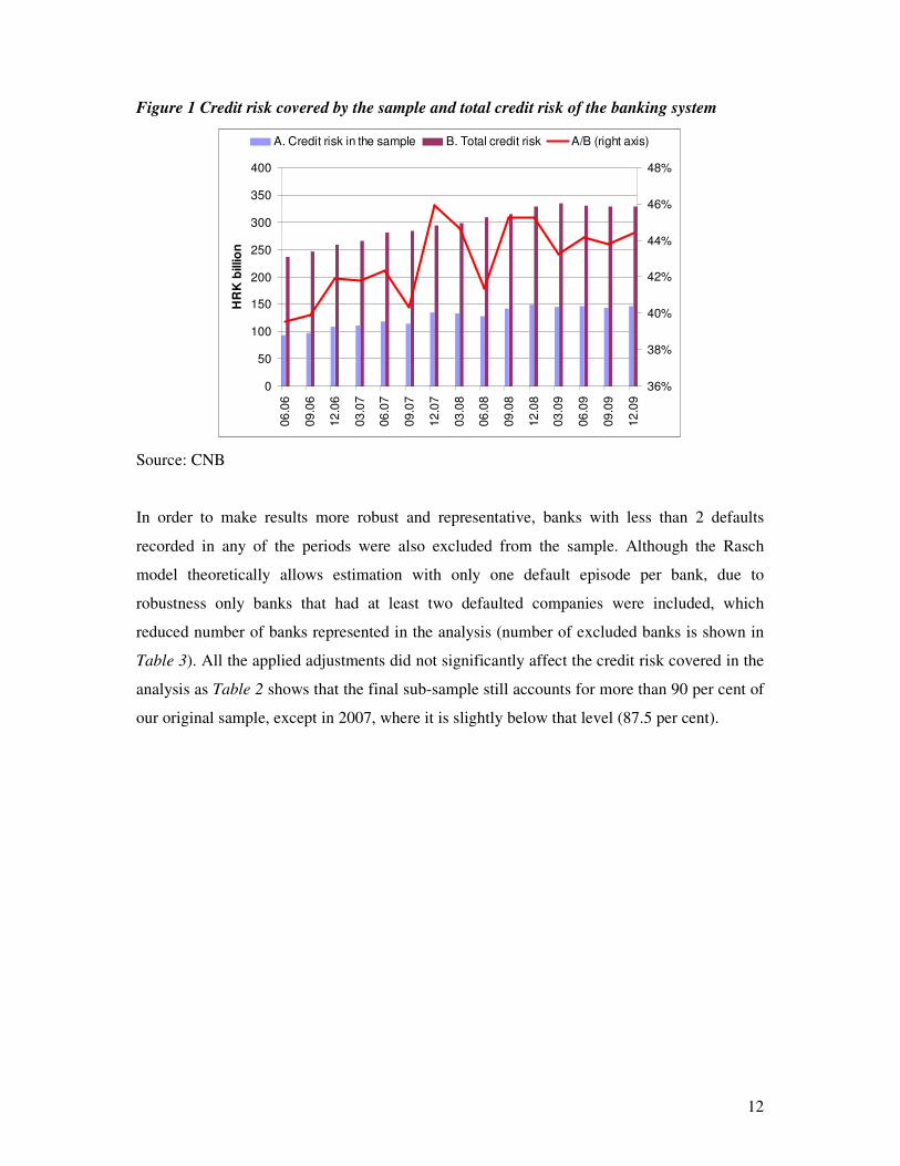
Figure 1 compares aggregate bank exposures towards companies in the sample with the totals

for the banking system. The database with detailed exposures recorded on a company basis

for each reporting bank contains a significant share of total credit risk in the banking system,

ranging from 40 to 45 per cent of the total credit risk. Cleaning of the sample for debtors

classified in public administration and defence, those classified as foreign entities and

financial intermediaries as well as any duplicate entries reduces the sample size a bit further.

Natural persons were also excluded from the analysis, while the sole proprietors were

maintained in the sample.

12

Figure 1 Credit risk covered by the sample and total credit risk of the banking system

0

50

100

150

200

250

300

350

400

06

.06

09

.06

12

.06

03

.07

06

.07

09

.07

12

.07

03

.08

06

.08

09

.08

12

.08

03

.09

06

.09

09

.09

12

.09

HR

K b

illio

n

36%

38%

40%

42%

44%

46%

48%

A. Credit risk in the sample B. Total credit risk A/B (right axis)

Source: CNB

In order to make results more robust and representative, banks with less than 2 defaults

recorded in any of the periods were also excluded from the sample. Although the Rasch

model theoretically allows estimation with only one default episode per bank, due to

robustness only banks that had at least two defaulted companies were included, which

reduced number of banks represented in the analysis (number of excluded banks is shown in

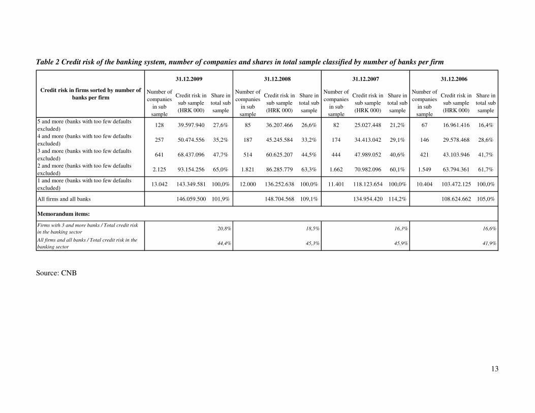
Table 3). All the applied adjustments did not significantly affect the credit risk covered in the

analysis as Table 2 shows that the final sub-sample still accounts for more than 90 per cent of

our original sample, except in 2007, where it is slightly below that level (87.5 per cent).

13

Table 2 Credit risk of the banking system, number of companies and shares in total sample classified by number of banks per firm

Number of

companies

in sub

sample

Credit risk in

sub sample

(HRK 000)

Share in

total sub

sample

Number of

companies

in sub

sample

Credit risk in

sub sample

(HRK 000)

Share in

total sub

sample

Number of

companies

in sub

sample

Credit risk in

sub sample

(HRK 000)

Share in

total sub

sample

Number of

companies

in sub

sample

Credit risk in

sub sample

(HRK 000)

Share in

total sub

sample

5 and more (banks with too few defaults

excluded)128 39.597.940 27,6% 85 36.207.466 26,6% 82 25.027.448 21,2% 67 16.961.416 16,4%

4 and more (banks with too few defaults

excluded)257 50.474.556 35,2% 187 45.245.584 33,2% 174 34.413.042 29,1% 146 29.578.468 28,6%

3 and more (banks with too few defaults

excluded)641 68.437.096 47,7% 514 60.625.207 44,5% 444 47.989.052 40,6% 421 43.103.946 41,7%

2 and more (banks with too few defaults

excluded)2.125 93.154.256 65,0% 1.821 86.285.779 63,3% 1.662 70.982.096 60,1% 1.549 63.794.361 61,7%

1 and more (banks with too few defaults

excluded)13.042 143.349.581 100,0% 12.000 136.252.638 100,0% 11.401 118.123.654 100,0% 10.404 103.472.125 100,0%

All firms and all banks 146.059.500 101,9% 148.704.568 109,1% 134.954.420 114,2% 108.624.662 105,0%

Memorandum items:

Firms with 3 and more banks / Total credit risk

in the banking sector20,8% 18,5% 16,3% 16,6%

All firms and all banks / Total credit risk in the

banking sector44,4% 45,3% 45,9% 41,9%

Credit risk in firms sorted by number of

banks per firm

31.12.200631.12.200731.12.200831.12.2009

Source: CNB

14

Table 2 showing the sample structure allows to tackle the trade off between the size of the sub

sample and the selected minimum number of banking links. The methodology applied to the

problem theoretically allows estimation by use of the two different banks per one company.

The choice was made to use only companies that have relations with at least 3 banks. This

increases robustness and minimises the probability that the company's credit risk will be

assessed by two similar, lenient or strict banks. Companies with 3 and more banks represent

more than 40 per cent of our total sample and from 16.6 in 2006 to 20.8 in 2009 per cent of

total credit risk of the banking system, which should be representative for most banks.

Table 2 also indicates that exposures of the banking system towards multiple borrowers have

increased more than the total credit risk, indicating perhaps increased competition that enables

companies to pick between banks as the number of companies with multiple bank relations

from the end of 2006 to the end of 2009 increasing more than the total number of companies

in the sample. This is particularly relevant for companies with four or more links, increasing

the number of average links with the banks.

Bank leniency and the application of the Rasch model

The bank has several options when a company defaults on its contractual loan payments. First

option is to seize the assets given as collateral, liquidate it and close the loan. The bank will

be more willing to embrace this option if the loan is well collateralized and the enforcement

of the liquidation is fast and straightforward. In addition to this, the bank has to think about

the reputation risk. If the bank forecloses on a company that faces temporary difficulties, it

might loose future income from this company and get a bad name in the business community.

So, if the collateral in not adequate, enforcement is slow or the bank cares about its reputation,

it might delay the process of downgrading the loan and initiating legal proceedings.

Additionally, downgrading a loan exerts negative influence on net income as it increases loan

loss provisions, or may even bite into the banks capitalization if a significant portion of the

loan portfolio is affected by downgrades. An attractive alternative to the loan downgrading

might be a loan renewal, where a new loan is issued instead of the old one or a loan is placed

under a moratorium.

As mentioned above, possible effects of collateral on loan classification pose the biggest

problem for the analysis. On the one hand, borrowers may be less inclined to perform a

15

strategic default on a well collateralized loan. On the other hand, bank holding a well

collateralised loan might be more willing to acknowledge a default and initiate a workout than

a bank that has a loan with no collateral. Our dataset unfortunately doesn't include collateral

information for each individual exposure so it is not possible to directly control for effects

arising from different loan collateralization. This might skew the results of our analysis and

tilt them towards measuring how well collateralised are loans instead of measuring bank

leniency or strictness, with the unknown possible direction of the effect. This issue is in part

tackled by using a strict definition of default: as mentioned above, as soon as non-payment in

excess of 90 days occurs, we designate the loan defaulted regardless of the expected loss.

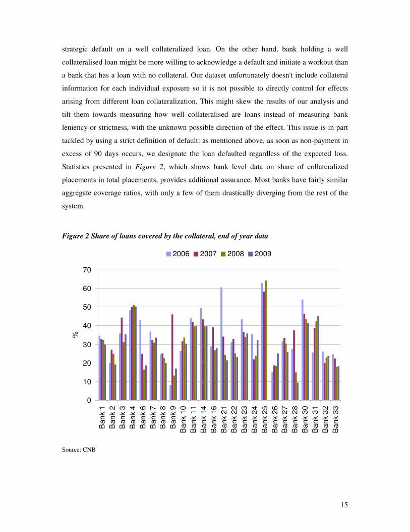
Statistics presented in Figure 2, which shows bank level data on share of collateralized

placements in total placements, provides additional assurance. Most banks have fairly similar

aggregate coverage ratios, with only a few of them drastically diverging from the rest of the

system.

Figure 2 Share of loans covered by the collateral, end of year data

0

10

20

30

40

50

60

70

Ban

k 1

Ban

k 2

Ban

k 3

Ban

k 4

Ban

k 6

Ban

k 7

Ban

k 8

Ban

k 9

Ba

nk 1

0

Ba

nk 1

1

Ba

nk 1

4

Ba

nk 1

6

Ba

nk 2

1

Ba

nk 2

2

Ba

nk 2

3

Ba

nk 2

4

Ba

nk 2

5

Ba

nk 2

6

Ba

nk 2

7

Ba

nk 2

8

Ba

nk 3

0

Ba

nk 3

1

Ba

nk 3

2

Ba

nk 3

3

%

2006 2007 2008 2009

Source: CNB

16

Furthermore, if collateral plays an important role in the loan classification, leniency /

strictness estimates shuld be correlated with the share of collateralised credits in credit

portfolio, i.e. the banks with significantly better collateralisation of portfolio will be rated

significantly stricter. This issue will be further examined bellow, in the results section.

From the literature presented in the introduction and the banks' incentive structure explained

above, it is obvious that the process of loan classification is far from being a well established

program with minimal human interaction. Just to the opposite, two banks might tend to

classify the same loan differently, according to their incentive structure.

The Rasch model enables ranking of the banks according to their strictness. The idea is to

treat banks as examiners and the companies as examinees. The company × bank matrix

described in the data section with a sample of loans to the same firms by multiple banks is a

starting point for the analysis that should give us the relative strictness / leniency estimate. For

example, if multiple banks have the loan to the same company in their books and all but one

bank designate the company defaulted, the conclusion is that the remaining bank is less strict

that the rest of the banks. The model enables us to do such comparison on a whole dataset and

extract the strictness / leniency estimate for each bank.

Estimation results are given in Table 3, where banks that are stricter from the average of the

system have estimates lower than 0 and banks that are more lenient than the average on the

system have estimates larger than 0. Changes in the score between years are not comparable,

because the estimation is performed on the data for every given year and the mean strictness /

leniency of the system which is a base for comparison can drift with time.

17

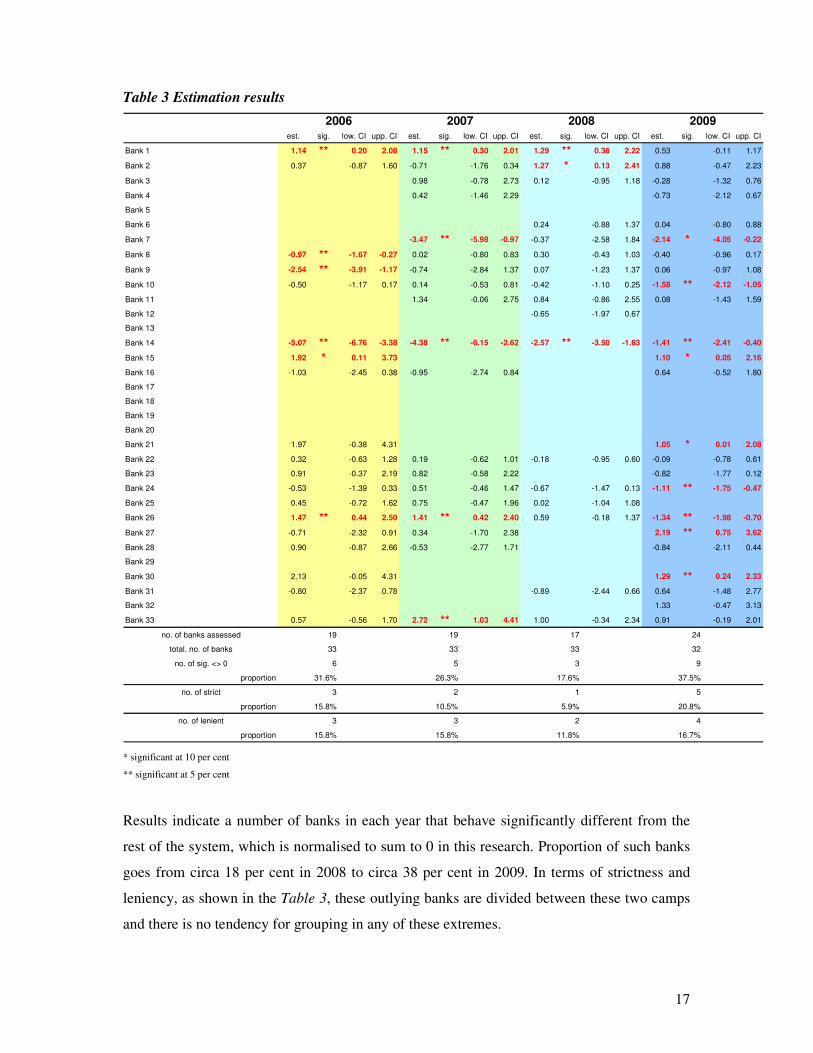
Table 3 Estimation results

est. sig. low. CI upp. CI est. sig. low. CI upp. CI est. sig. low. CI upp. CI est. sig. low. CI upp. CI

Bank 1 1.14 ** 0.20 2.08 1.15 ** 0.30 2.01 1.29 ** 0.36 2.22 0.53 -0.11 1.17

Bank 2 0.37 -0.87 1.60 -0.71 -1.76 0.34 1.27 * 0.13 2.41 0.88 -0.47 2.23

Bank 3 0.98 -0.78 2.73 0.12 -0.95 1.18 -0.28 -1.32 0.76

Bank 4 0.42 -1.46 2.29 -0.73 -2.12 0.67

Bank 5

Bank 6 0.24 -0.88 1.37 0.04 -0.80 0.88

Bank 7 -3.47 ** -5.98 -0.97 -0.37 -2.58 1.84 -2.14 * -4.05 -0.22

Bank 8 -0.97 ** -1.67 -0.27 0.02 -0.80 0.83 0.30 -0.43 1.03 -0.40 -0.96 0.17

Bank 9 -2.54 ** -3.91 -1.17 -0.74 -2.84 1.37 0.07 -1.23 1.37 0.06 -0.97 1.08

Bank 10 -0.50 -1.17 0.17 0.14 -0.53 0.81 -0.42 -1.10 0.25 -1.58 ** -2.12 -1.05

Bank 11 1.34 -0.06 2.75 0.84 -0.86 2.55 0.08 -1.43 1.59

Bank 12 -0.65 -1.97 0.67

Bank 13

Bank 14 -5.07 ** -6.76 -3.38 -4.38 ** -6.15 -2.62 -2.57 ** -3.50 -1.63 -1.41 ** -2.41 -0.40

Bank 15 1.92 * 0.11 3.73 1.10 * 0.05 2.16

Bank 16 -1.03 -2.45 0.38 -0.95 -2.74 0.84 0.64 -0.52 1.80

Bank 17

Bank 18

Bank 19

Bank 20

Bank 21 1.97 -0.38 4.31 1.05 * 0.01 2.08

Bank 22 0.32 -0.63 1.28 0.19 -0.62 1.01 -0.18 -0.95 0.60 -0.09 -0.78 0.61

Bank 23 0.91 -0.37 2.19 0.82 -0.58 2.22 -0.82 -1.77 0.12

Bank 24 -0.53 -1.39 0.33 0.51 -0.46 1.47 -0.67 -1.47 0.13 -1.11 ** -1.75 -0.47

Bank 25 0.45 -0.72 1.62 0.75 -0.47 1.96 0.02 -1.04 1.08

Bank 26 1.47 ** 0.44 2.50 1.41 ** 0.42 2.40 0.59 -0.18 1.37 -1.34 ** -1.98 -0.70

Bank 27 -0.71 -2.32 0.91 0.34 -1.70 2.38 2.19 ** 0.75 3.62

Bank 28 0.90 -0.87 2.66 -0.53 -2.77 1.71 -0.84 -2.11 0.44

Bank 29

Bank 30 2.13 -0.05 4.31 1.29 ** 0.24 2.33

Bank 31 -0.80 -2.37 0.78 -0.89 -2.44 0.66 0.64 -1.48 2.77

Bank 32 1.33 -0.47 3.13

Bank 33 0.57 -0.56 1.70 2.72 ** 1.03 4.41 1.00 -0.34 2.34 0.91 -0.19 2.01

no. of banks assessed 19 19 17 24

total. no. of banks 33 33 33 32

no. of sig. <> 0 6 5 3 9

proportion 31.6% 26.3% 17.6% 37.5%

no. of strict 3 2 1 5

proportion 15.8% 10.5% 5.9% 20.8%

no. of lenient 3 3 2 4

proportion 15.8% 15.8% 11.8% 16.7%

2006 2007 2008 2009

* significant at 10 per cent

** significant at 5 per cent

Results indicate a number of banks in each year that behave significantly different from the

rest of the system, which is normalised to sum to 0 in this research. Proportion of such banks

goes from circa 18 per cent in 2008 to circa 38 per cent in 2009. In terms of strictness and

leniency, as shown in the Table 3, these outlying banks are divided between these two camps

and there is no tendency for grouping in any of these extremes.

18

Although the results are not directly comparable from year to year, i.e. we can not say that the

Bank 26 is significantly stricter in 2009 than 2008, we can compare the relative position of

that bank. For example, this bank has migrated from being more lenient than average to being

stricter than average of the banking system. On a year to year basis, the results are generally

stable as there are no major jumps from severe strictness to extreme leniency which indicates

that the majority of the banks change their loan assessment and risk management practices

slowly or in line with the rest of the system. This also gives indication of the robustness of the

model.

Results for the 2009 are particularly interesting. In the year when the economic activity

contracted significantly, and share of bad loans in the books of the banks expectedly

increased, the dispersion of strictness / leniency scores of the banks increased, with proportion

of strict banks increasing to historical high, reversing the trend observed in the data since

2006. This indicates that the banks pursued two different strategies after the crises broke out.

The first one was to acknowledge the rise in proportion of bad loans and initiate downgrades,

which is reflected in the increase in the number of strict banks. The other was to keep to

business as usual and try to keep loans in the highest category for as long as possible.

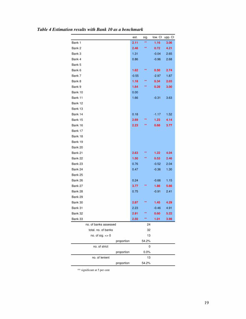
As a matter of comparison it is possible to select any bank as a baseline. In that case the

results will show how other banks in the system compare to that bank. Picking a bank whose

rating system is deemed adequate and contrast it with other banks might be a useful exercise.

Table 4 shows how the comparison with Bank 10 looks in 2009. Results show that circa 54

per cent of the banks is more lenient than Bank 10. If we have had chosen Bank 10 as optimal

good practice example, many banks in the system require tougher standards.

19

Table 4 Estimation results with Bank 10 as a benchmark

est. sig. low. CI upp. CI

Bank 1 2.11 ** 1.16 3.06

Bank 2 2.46 ** 0.72 4.21

Bank 3 1.31 -0.04 2.65

Bank 4 0.86 -0.96 2.68

Bank 5

Bank 6 1.62 ** 0.50 2.74

Bank 7 -0.55 -2.97 1.87

Bank 8 1.18 ** 0.34 2.03

Bank 9 1.64 ** 0.28 3.00

Bank 10 0.00

Bank 11 1.66 -0.31 3.63

Bank 12

Bank 13

Bank 14 0.18 -1.17 1.52

Bank 15 2.69 ** 1.23 4.14

Bank 16 2.23 ** 0.68 3.77

Bank 17

Bank 18

Bank 19

Bank 20

Bank 21 2.63 ** 1.22 4.04

Bank 22 1.50 ** 0.53 2.46

Bank 23 0.76 -0.52 2.04

Bank 24 0.47 -0.36 1.30

Bank 25

Bank 26 0.24 -0.66 1.15

Bank 27 3.77 ** 1.88 5.66

Bank 28 0.75 -0.91 2.41

Bank 29

Bank 30 2.87 ** 1.45 4.29

Bank 31 2.23 -0.46 4.91

Bank 32 2.91 ** 0.60 5.22

Bank 33 2.50 ** 1.01 3.98

no. of banks assessed 24

total. no. of banks 32

no. of sig. <> 0 13

proportion 54.2%

no. of strict 0

proportion 0.0%

no. of lenient 13

proportion 54.2%

** significant at 5 per cent

20

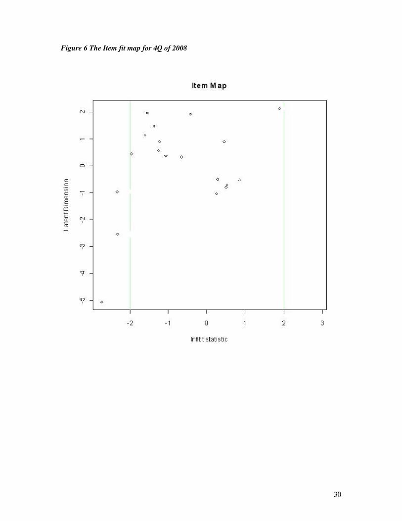
The Model Robustness

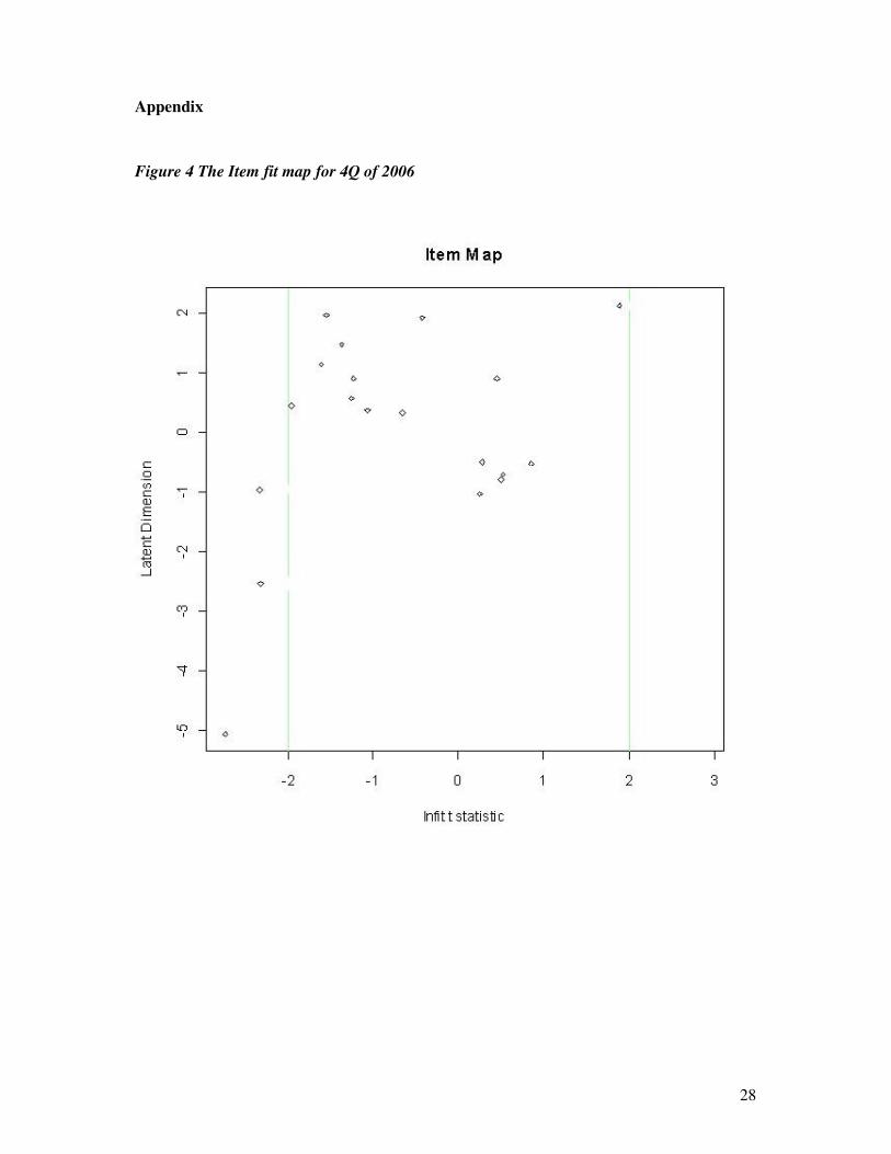
There are several factors that could potentially affect the interpretation of the results. First,

data structure may not be appropriate for application of the Rasch model. Popular way to test

the applicability of the Rasch model to the data at hand is by constructing so called maps,

where the vertical axis shows strictness / leniency estimate and horizontal axis measures

misfit. The misfit is defined as a sum of squared differences between the observed and

expected pattern if the bank rated all the companies in line with its relative leniency /

strictness estimate. In that respect, the misfit can be in two directions, i.e. recorded data can be

too random for Rasch model or too deterministic (too close to Guttman response pattern). In

both cases the test statistic will indicate a misfit, in the first case, the fit statistic will be

negative, indicating too deterministic response pattern ("overfit" of the data to the model) and

in other case the statistic will be positive, indicating pattern that is more random than the

Rasch model expects, basically unpredictable ("underfit"). As it is explained in Bond and Fox

(2001) the fit statistics can be transformed to approximately normalized t distribution, where

t>2 indicates an underfit of the model and t<-2 overfit of the model at 5 per cent significance

level.

Figures 4 to 7 in the Appendix show how the Rasch model fits our dataset. In all four periods

only a few banks lie outside of the 95% confidence interval proposed by the Rasch model.

Having said that, it is important to note that most of the misfitting banks are in the overfit

region, indicating that they closely follow the Guttman structure, meaning that if they are

strict they rate majority of their loans defaulted (significantly more than Rasch model would

predict) and if they are lenient, they rate majority of their clients as standard loans (again,

significantly more than the Rasch model predicts). Another way to interpret misfitting banks

it to treat over fitting banks as completely coherent with the rest of the banking system and

their measured leniency / strictness in an almost deterministic (i.e. they are always more

lenient than some stricter bank and vice versa) and to treat underfitting banks as giving marks

randomly, completely different than all other banks in the system.

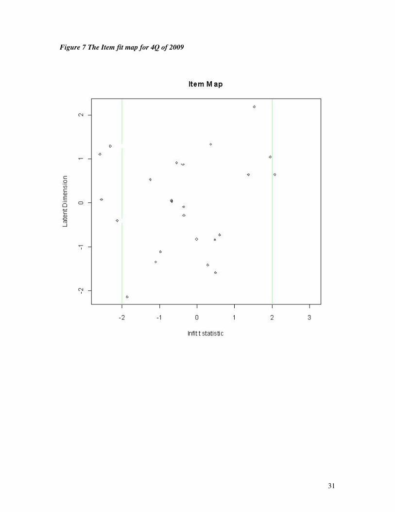
End 2009 (Figure 7) is particularly interesting period for close examination. In that period we

see the largest number of misfitting banks (5). Most of them (4) are in the region of overfit,

indicating they are close to the Guttman structure, i.e. their behaviour is non random, and the

categorization of the loans is coherent with the rest of the banking system. One bank is in the

21

region of underfit, indicating that categorization of the loans in its portfolio resembles a

random process, which is a case for Bank 31. Possible interpretation is that as a result of the

crisis and increases in the share of non-performing loans in their portfolios these banks started

re-rating larger proportions of their portfolios and they did that in line with their relative

strictness. In the data this was observed as a move from the middle ground, where some loans

were rated randomly (compared to the Guttman structure) to rating greater proportion of the

loans as their strictness / leniency rating suggests. If the banks were strict before (comparing

to other banks), on a smaller portion of their portfolio, now they are stricter on a larger

proportion of their portfolio, so the difference between idealistic Guttman structure and real

data is smaller. Similarly, if the banks were more lenient than other banks, as the proportion

of the overall portfolio that is being re-rated by the banks increases, and some banks kept their

lenient approach, they move closer to the idealistic Guttman pattern. The banks that are in this

region of overfit in 2009 are Bank 30, Bank 15, Bank 11 and Bank 8.

The issue arising from the impact of collateral on loan classification was already discussed

earlier. Correlations between the loan coverage ratio and strictness / leniency estimate for the

complete sample should give some indication on the relevance of that issue (Figure 3).

22

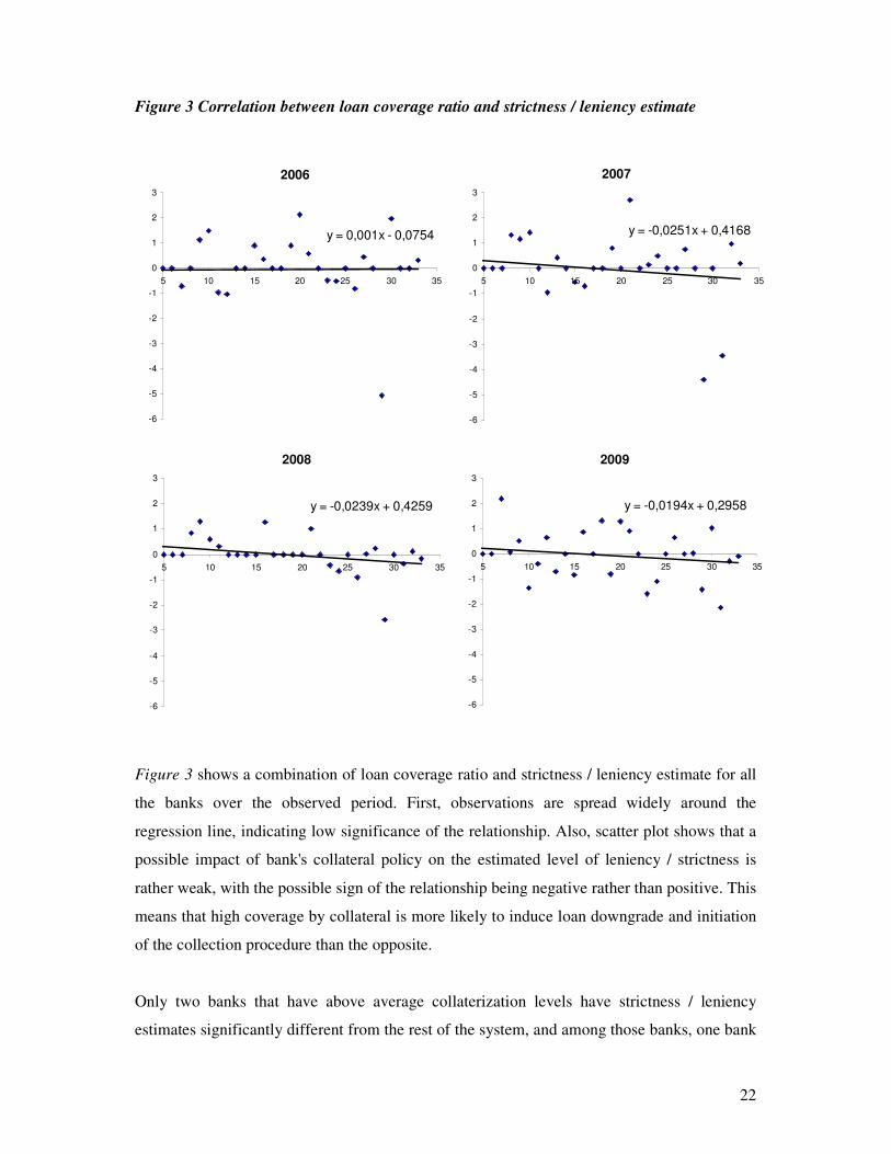
Figure 3 Correlation between loan coverage ratio and strictness / leniency estimate

2006

y = 0,001x - 0,0754

-6

-5

-4

-3

-2

-1

0

1

2

3

5 10 15 20 25 30 35

2009

y = -0,0194x + 0,2958

-6

-5

-4

-3

-2

-1

0

1

2

3

5 10 15 20 25 30 35

2007

y = -0,0251x + 0,4168

-6

-5

-4

-3

-2

-1

0

1

2

3

5 10 15 20 25 30 35

2008

y = -0,0239x + 0,4259

-6

-5

-4

-3

-2

-1

0

1

2

3

5 10 15 20 25 30 35

Figure 3 shows a combination of loan coverage ratio and strictness / leniency estimate for all

the banks over the observed period. First, observations are spread widely around the

regression line, indicating low significance of the relationship. Also, scatter plot shows that a

possible impact of bank's collateral policy on the estimated level of leniency / strictness is

rather weak, with the possible sign of the relationship being negative rather than positive. This

means that high coverage by collateral is more likely to induce loan downgrade and initiation

of the collection procedure than the opposite.

Only two banks that have above average collaterization levels have strictness / leniency

estimates significantly different from the rest of the system, and among those banks, one bank

23

is significantly more strict that the system and the other one is significantly more lenient than

the rest of the system (Bank 14 and Bank 30). Among the banks with the loan portfolio

substantially less collateralized than the rest of the system, only one bank (Bank 9) is

significantly different from the rest of the system being stricter and that happens in the year

when its coverage ratio is lowest in the sample.

24

Conclusion and potential application of results

Bad loans and provisions have been in the core of interest of both central bankers, commercial

banks, governments and general public in many countries around the world for some time

now. The model presented here should give additional information to central bank's prudential

department and management on the reliability of risk classification systems used by most

banks, but also to commercial bankers.

Analyzing the data and thinking about it in terms of Rasch model gives an excellent way to

aggregate available information about banks' approaches to classification of credit risk. The

sole process of preparing the data for the analysis is useful as it opens the new way to thinking

as interrelations between banks are used. The results of the model, where the most lenient

banks are singled out and all banks are ordered by their leniency give an excellent starting

point for concentration of surveillance efforts so that supervision can focus on credit

classification and risk management in the most lenient banks. Furthermore, the instances

where the classification of specific companies differs can be explored in detail, within a single

bank as well as between different banks. Also, if structure of the defaults for some banks

deviates from the expected, although it does not necessarily have to be lenient, it may indicate

potential problems with risk classification. Additionally, the sole fact that not all banks can

enter the analysis because they have too few defaults in the sample that includes only firms

rated by multiple banks is an obvious indication for further analysis of that bank loan portfolio

and risk management and credit classification system.

In addition to providing valuable information for performing the supervisory function, the

results can also aid the assessment of financial stability of the banking system as they allow

quick assessment of the risk management practices in the banking system. Specific bank for

which the risk management practices are regarded adequate can be used as an anchor and

what-if analysis can be performed - what would happen with the bad loans of the banking

system if the risk management practices of that bank were applied throughout the system?

This would give an indication of the potential extent of manipulations with loan classification

in the banks' books and allow the analyst to estimate "true" amount of bad loans. In the

appendix I explore a possible way to achieve that.

25

The area with big future potential for methods based on the Rasch model is comparison of

credit risk assessment systems. As literature surveyed in first section shows, the comparison

of credit rating systems is a big and interesting topic for central and commercial banking.

Basel accord stimulates banks to use internal ratings and rely on those in order to determine

needed capital. Under such an approach to capital allocation, better internal credit risk system

will be a comparative advantage for the bank as it will optimize the amount of capital. The

Rasch model can be applied to that problem and rating systems between two banks can be

compared quickly and efficiently, so banks whose rating system are considered sufficiently

good may be benchmarked against other banks.

26

Literature

Alagumalai, S., Curtis, D. D., Hungi, N. (2005) Applied Rasch Measurement: A Book of

Exemplars: Papers in Honour of John P. Keeves (Education in the Asia-Pacific Region:

Issues, Concerns and Prospects), Springer

Bond, T. G., Fox C. M. (2001) Applying the Rasch Model : Fundamental Measurement in the

Human Sciences, Lawrence Erlbaum Associates, Inc.

Caballero, R. J., Hoshi, T., Kashyap, A. K. (2008) Zombie Lending and Depressed

Restructuring in Japan, American Economic Review, 98:5, 1943-1977

Cantor, R. and Packer F. (1997), Differences of Opinion and Selection Bias in the Credit

Rating Industry, Journal of Banking and Finance 21, 1395-1417

Carey, M. (1998) Credit Risk in Private Debt Portfolios, Journal of Finance, Vol. LIII, 1363-

1387

Carey, M. (2001) Some Evidence on the Consistency of Banks’ Internal Credit Ratings,

mimeo

Carriquiry, A. L., Fienberg, S. E., (2005) Rasch models in Armitage, P., Colton, T.,

Encyclopedia of Biostatistics, Wiley

Hornik, K., Jankowitsch, R., Leitner, C., Lingo, M., Pichler, S., Winkler, G. (2010) A latent

variable approach to validate credit rating systems. In Daniel Rösch and Harald Scheule,

editors, Model Risk in Financial Crises, pages 277-296. Risk Books, London

Hornik, K., Jankowitsch, R., Lingo, M., Pichler, S., Winkler, G. (2007) Validation of Credit

Rating Systems Using Multi-Rater Information, Journal of Credit Risk, Volume 3, Number 4

Jacobson, T., Lindé, J., Roszbach, K. F. (2005) Internal Ratings Systems, Implied Credit Risk

and the Consistency of Banks' Risk Classification Policies. Journal of Banking and Finance,

Forthcoming; Riksbank Working Paper No. 155

Laurin A., and Majnoni G. (2003) Bank Loan Classification and Provisioning Practices in

Selected Developed and Emerging Countries, World Bank working paper no. 1

Liu, C. C. and Ryan, S.G. (2003) Income Smoothing over the Business Cycle: Changes in

Banks’ Coordinated Management of Provisions for Loan Losses and Loan Charge-offs from

the Pre-1990 Bust to the 1990s Boom, NYU Stern Working Paper Series S-CDM-03-15

Mair P., Hatzinger R., Maier, M. (2010) Extended Rasch Modeling: The R Package eRm

Mair, P., and Hatzinger, R. (2007) Extended Rasch modeling: The eRm package for the

application of IRT models in R, Journal of Statistical Software, 20(9), 1-20.

Odluka o adekvatnosti jamstvenoga kapitala kreditnih institucija (Official Gazzete no. 1/09.,

75/09. i 2/10.

Odluka o klasifikaciji plasmana i izvanbilančnih obveza banaka (Official Gazette no. 1/2009.,

75/2009. and 2/2010)

27

R Development Core Team (2010). R: A language and environment for statistical computing.

R Foundation for Statistical Computing, Vienna, Austria. ISBN 3-900051-07-0, URL

http://www.R-project.org/

Song, I. (2002) Collateral in Loan Classification and Provisioning, IMF Working Paper

WP/02/122

Stahl, J., Bergstrom, B., Gershon, R. (2000) CAT Administration of Language Placement

Examinations Journal of Applied Measurement, 1(3), 292-302

28

Appendix

Figure 4 The Item fit map for 4Q of 2006

29

Figure 5 The Item fit map for 4Q of 2007

30

Figure 6 The Item fit map for 4Q of 2008

31

Figure 7 The Item fit map for 4Q of 2009

32

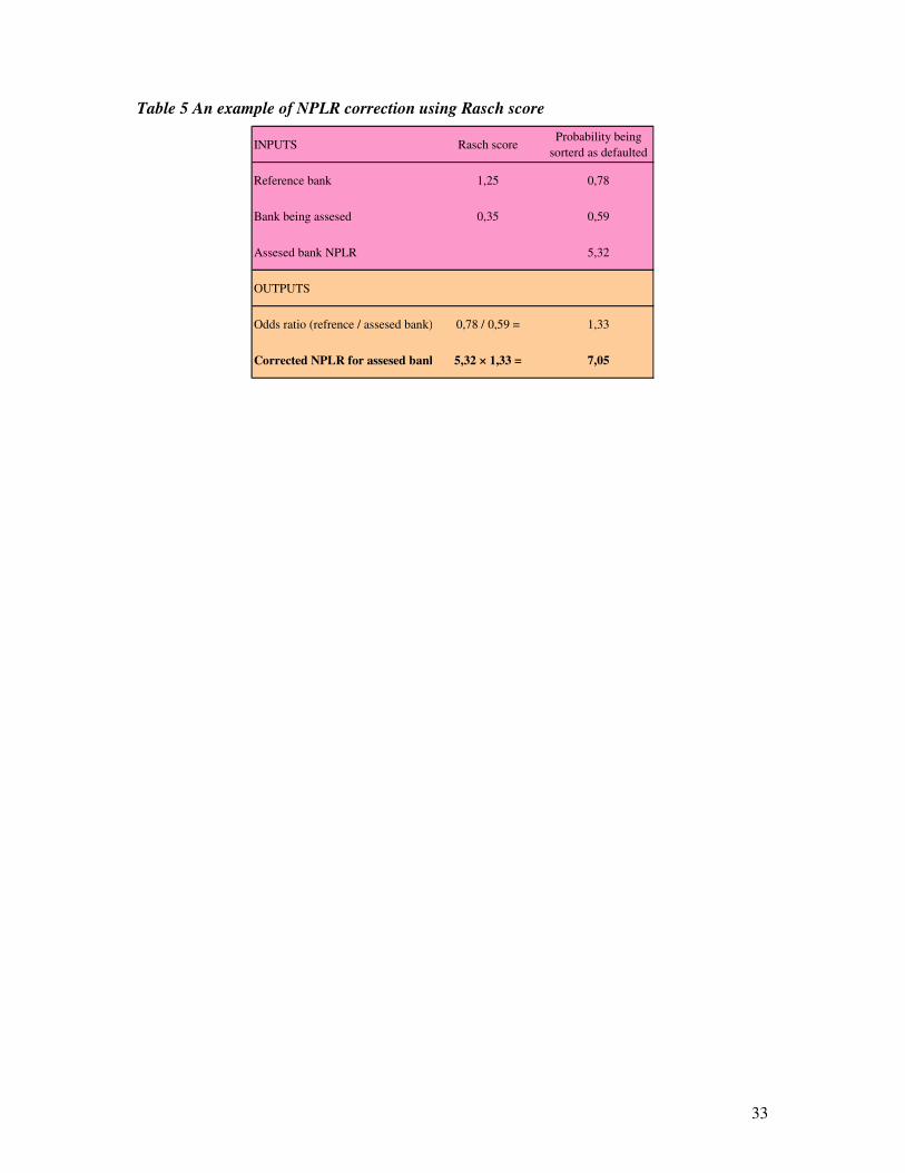
How to obtain corrected NPL ratios using strictness / leniency estimate?

One possible step forward is to use estimated strictness / leniency estimates in order to correct

non performing loan ratios by using relative strictness / leniency estimate. The share of non-

performing loans was revised up for banks less strict than the reference bank, while it was

revised down for stricter banks. Reference bank can be picked on the basis of a priori

knowledge of risk management quality.

As explained above, the scores from Rasch analysis are log odds, so we can obtain estimated

probabilities from the Rasch estimate. For example, using log odds calculation Rasch score of

2.20 transforms roughly to a probability of 90 per cent of being rated defaulted (the natural

logarithm of 0.9/0.1=2.20) which should be compared to the default probability of 50 per cent

for the average bank in the system (the natural logarithm of 0.5/0.5=0). If the same

transformation is applied to a reference bank and any other banks, we can use their odds ratio

to correct the non-performing loan ratio, where we can put the reference bank in the

numerator and the bank to which we are applying correction in the denominator. If the odds

ratio is 1 this implies similar probability of being sorted as non performing in both banks, if

this ratio is higher than 1, the probability of being sorted as non-performing in the reference

bank is higher and vice versa in case where the ratio is less than 1. For example we would

interpret the odds ratio of 2, as that the placement is 2 times more likely to be classified as bad

in the reference bank that in the bank being assessed. We can use that line of reasoning to

obtain the correction, for non performing loans ratio (NPLR), and new, corrected NPLR for

the bank being would be 2 × original NPLR. Table 5 gives an example correction of NPLR

based on a Rasch leniency / strictness estimate.

33

Table 5 An example of NPLR correction using Rasch score

INPUTS Rasch scoreProbability being

sorterd as defaulted

Reference bank 1,25 0,78

Bank being assesed 0,35 0,59

Assesed bank NPLR 5,32

OUTPUTS

Odds ratio (refrence / assesed bank) 0,78 / 0,59 = 1,33

Corrected NPLR for assesed bank 5,32 × 1,33 = 7,05