Published in Image Processing On Line on 2014–06–26.Submitted on 2013–08–31, accepted on 2014–05–09.ISSN 2105–1232 c© 2014 IPOL & the authors CC–BY–NC–SAThis article is available online with supplementary materials,software, datasets and online demo athttp://dx.doi.org/10.5201/ipol.2014.104

2014/07/01

v0.5

IPOL

article

class

An Analysis of the Viola-Jones Face Detection Algorithm

Yi-Qing Wang

CMLA, ENS Cachan, France (yiqing.wang@cmla.ens-cachan.fr)

Abstract

In this article, we decipher the Viola-Jones algorithm, the first ever real-time face detectionsystem. There are three ingredients working in concert to enable a fast and accurate detection:the integral image for feature computation, Adaboost for feature selection and an attentionalcascade for efficient computational resource allocation. Here we propose a complete algorithmicdescription, a learning code and a learned face detector that can be applied to any color image.Since the Viola-Jones algorithm typically gives multiple detections, a post-processing step isalso proposed to reduce detection redundancy using a robustness argument.

Source Code

The source code and the online demo are accessible at the IPOL web page of this article1.

Keywords: face detection; Viola-Jones algorithm; integral image; Adaboost

1 Introduction

A face detector has to tell whether an image of arbitrary size contains a human face and if so, whereit is. One natural framework for considering this problem is that of binary classification, in whicha classifier is constructed to minimize the misclassification risk. Since no objective distribution candescribe the actual prior probability for a given image to have a face, the algorithm must minimizeboth the false negative and false positive rates in order to achieve an acceptable performance.

This task requires an accurate numerical description of what sets human faces apart from otherobjects. It turns out that these characteristics can be extracted with a remarkable committee learn-ing algorithm called Adaboost, which relies on a committee of weak classifiers to form a strongone through a voting mechanism. A classifier is weak if, in general, it cannot meet a predefinedclassification target in error terms.

An operational algorithm must also work with a reasonable computational budget. Techniquessuch as integral image and attentional cascade make the Viola-Jones algorithm [10] highly efficient:fed with a real time image sequence generated from a standard webcam, it performs well on astandard PC.

1http://dx.doi.org/10.5201/ipol.2014.104

Yi-Qing Wang, An Analysis of the Viola-Jones Face Detection Algorithm, Image Processing On Line, 4 (2014), pp. 128–148.http://dx.doi.org/10.5201/ipol.2014.104

An Analysis of the Viola-Jones Face Detection Algorithm

2 Algorithm

To study the algorithm in detail, we start with the image features for the classification task.

2.1 Features and Integral Image

The Viola-Jones algorithm uses Haar-like features, that is, a scalar product between the image andsome Haar-like templates. More precisely, let I and P denote an image and a pattern, both of thesame size N ×N (see Figure 1). The feature associated with pattern P of image I is defined by∑

1≤i≤N

∑1≤j≤N

I(i, j)1P (i,j) is white −∑

1≤i≤N

∑1≤j≤N

I(i, j)1P (i,j) is black.

To compensate the effect of different lighting conditions, all the images should be mean andvariance normalized beforehand. Those images with variance lower than one, having little informationof interest in the first place, are left out of consideration.

(a) (b) (c)

Figure 1: Haar-like features. Here as well as below, the background of a template like (b) is paintedgray to highlight the pattern’s support. Only those pixels marked in black or white are used whenthe corresponding feature is calculated.

(a) (b) (c) (d) (e)

Figure 2: Five Haar-like patterns. The size and position of a pattern’s support can vary providedits black and white rectangles have the same dimension, border each other and keep their relativepositions. Thanks to this constraint, the number of features one can draw from an image is somewhatmanageable: a 24 × 24 image, for instance, has 43200, 27600, 43200, 27600 and 20736 features ofcategory (a), (b), (c), (d) and (e) respectively, hence 162336 features in all.

In practice, five patterns are considered (see Figure 2 and Algorithm 1). The derived featuresare assumed to hold all the information needed to characterize a face. Since faces are by and largeregular by nature, the use of Haar-like patterns seems justified. There is, however, another crucialelement which lets this set of features take precedence: the integral image which allows to calculatethem at a very low computational cost. Instead of summing up all the pixels inside a rectangular

129

Yi-Qing Wang

Algorithm 1 Computing a 24× 24 image’s Haar-like feature vector

1: Input: a 24× 24 image with zero mean and unit variance2: Output: a d× 1 scalar vector with its feature index f ranging from 1 to d3: Set the feature index f← 04: Compute feature type (a)5: for all (i, j) such that 1 ≤ i ≤ 24 and 1 ≤ j ≤ 24 do6: for all (w, h) such that i+ h− 1 ≤ 24 and j + 2w − 1 ≤ 24 do7: compute the sum S1 of the pixels in [i, i+ h− 1]× [j, j + w − 1]8: compute the sum S2 of the pixels in [i, i+ h− 1]× [j + w, j + 2w − 1]9: record this feature parametrized by (1, i, j, w, h): S1 − S2

10: f← f + 111: end for12: end for13: Compute feature type (b)14: for all (i, j) such that 1 ≤ i ≤ 24 and 1 ≤ j ≤ 24 do15: for all (w, h) such that i+ h− 1 ≤ 24 and j + 3w − 1 ≤ 24 do16: compute the sum S1 of the pixels in [i, i+ h− 1]× [j, j + w − 1]17: compute the sum S2 of the pixels in [i, i+ h− 1]× [j + w, j + 2w − 1]18: compute the sum S3 of the pixels in [i, i+ h− 1]× [j + 2w, j + 3w − 1]19: record this feature parametrized by (2, i, j, w, h): S1 − S2 + S320: f← f + 121: end for22: end for23: Compute feature type (c)24: for all (i, j) such that 1 ≤ i ≤ 24 and 1 ≤ j ≤ 24 do25: for all (w, h) such that i+ 2h− 1 ≤ 24 and j + w − 1 ≤ 24 do26: compute the sum S1 of the pixels in [i, i+ h− 1]× [j, j + w − 1]27: compute the sum S2 of the pixels in [i+ h, i+ 2h− 1]× [j, j + w − 1]28: record this feature parametrized by (3, i, j, w, h): S1 − S229: f← f + 130: end for31: end for32: Compute feature type (d)33: for all (i, j) such that 1 ≤ i ≤ 24 and 1 ≤ j ≤ 24 do34: for all (w, h) such that i+ 3h− 1 ≤ 24 and j + w − 1 ≤ 24 do35: compute the sum S1 of the pixels in [i, i+ h− 1]× [j, j + w − 1]36: compute the sum S2 of the pixels in [i+ h, i+ 2h− 1]× [j, j + w − 1]37: compute the sum S3 of the pixels in [i+ 2h, i+ 3h− 1]× [j, j + w − 1]38: record this feature parametrized by (4, i, j, w, h): S1 − S2 + S339: f← f + 140: end for41: end for42: Compute feature type (e)43: for all (i, j) such that 1 ≤ i ≤ 24 and 1 ≤ j ≤ 24 do44: for all (w, h) such that i+ 2h− 1 ≤ 24 and j + 2w − 1 ≤ 24 do45: compute the sum S1 of the pixels in [i, i+ h− 1]× [j, j + w − 1]46: compute the sum S2 of the pixels in [i+ h, i+ 2h− 1]× [j, j + w − 1]47: compute the sum S3 of the pixels in [i, i+ h− 1]× [j + w, j + 2w − 1]48: compute the sum S4 of the pixels in [i+ h, i+ 2h− 1]× [j + w, j + 2w − 1]49: record this feature parametrized by (5, i, j, w, h): S1 − S2 − S3 + S450: f← f + 151: end for

52: end for

130

An Analysis of the Viola-Jones Face Detection Algorithm

window, this technique mirrors the use of cumulative distribution functions. The integral image IIof I

II(i, j) :=

{∑1≤s≤i

∑1≤t≤j I(s, t), 1 ≤ i ≤ N and 1 ≤ j ≤ N

0, otherwise,

is so defined that∑N1≤i≤N2

∑N3≤j≤N4

I(i, j) = II(N2, N4)− II(N2, N3 − 1)− II(N1 − 1, N4) + II(N1 − 1, N3 − 1), (1)

holds for all N1 ≤ N2 and N3 ≤ N4. As a result, computing an image’s rectangular local sum requiresat most four elementary operations given its integral image. Moreover, obtaining the integral imageitself can be done in linear time: setting N1 = N2 and N3 = N4 in (1), we find

I(N1, N3) = II(N1, N3)− II(N1, N3 − 1)− II(N1 − 1, N3) + II(N1 − 1, N3 − 1).

Hence a recursive relation which leads to Algorithm 2.

Algorithm 2 Integral Image

1: Input: an image I of size N ×M .2: Output: its integral image II of the same size.3: Set II(1, 1) = I(1, 1).4: for i = 1 to N do5: for j = 1 to M do6: II(i, j) = I(i, j) + II(i, j − 1) + II(i − 1, j) − II(i − 1, j − 1) and II is defined to be zero

whenever its argument (i, j) ventures out of I’s domain.7: end for8: end for

As a side note, let us mention that once the useful features have been selected by the boostingalgorithm, one needs to scale them up accordingly when dealing with a bigger window (see Algo-rithm 3). Smaller windows, however, will not be looked at.

2.2 Feature Selection with Adaboost

How to make sense of these features is the focus of Adaboost [1].Some terminology. A classifier maps an observation to a label valued in a finite set. For face

detection, it assumes the form of f : Rd 7→ {−1, 1}, where 1 means that there is a face and −1 thecontrary (see Figure 3) and d is the number of Haar-like features extracted from an image. Giventhe probabilistic weights w· ∈ R+ assigned to a training set made up of n observation-label pairs(xi, yi), Adaboost aims to iteratively drive down an upper bound of the empirical loss

n∑i=1

wi1yi 6=f(xi),

under mild technical conditions (see Appendix A). Remarkably, the decision rule constructed byAdaboost remains reasonably simple so that it is not prone to overfitting, which means that theempirically learned rule often generalizes well. For more details on the method, we refer to [2, 3].Despite its groundbreaking success, it ought to be said that Adaboost does not learn what a face

131

Yi-Qing Wang

Algorithm 3 Feature Scaling

1: Input: an e× e image with zero mean and unit variance (e ≥ 24)2: Parameter: a Haar-like feature type and its parameter (i, j, w, h) as defined in Algorithm 13: Output: the feature value4: if feature type (a) then5: set the original feature support size a← 2wh6: i← Jie/24K, j ← Jje/24K, h← Jhe/24K where JzK defines the nearest integer to z ∈ R+

7: w ← max{κ ∈ N : κ ≤ J1 + 2we/24K/2, 2κ ≤ e− j + 1}8: compute the sum S1 of the pixels in [i, i+ h− 1]× [j, j + w − 1]9: compute the sum S2 of the pixels in [i, i+ h− 1]× [j + w, j + 2w − 1]

10: return the scaled feature (S1−S2)a2wh

11: end if12: if feature type (b) then13: set the original feature support size a← 3wh14: i← Jie/24K, j ← Jje/24K, h← Jhe/24K15: w ← max{κ ∈ N : κ ≤ J1 + 3we/24K/3, 3κ ≤ e− j + 1}16: compute the sum S1 of the pixels in [i, i+ h− 1]× [j, j + w − 1]17: compute the sum S2 of the pixels in [i, i+ h− 1]× [j + w, j + 2w − 1]18: compute the sum S2 of the pixels in [i, i+ h− 1]× [j + 2w, j + 3w − 1]

19: return the scaled feature (S1−S2+S3)a3wh

20: end if21: if feature type (c) then22: set the original feature support size a← 2wh23: i← Jie/24K, j ← Jje/24K, w ← Jwe/24K24: h← max{κ ∈ N : κ ≤ J1 + 2he/24K/2, 2κ ≤ e− i+ 1}25: compute the sum S1 of the pixels in [i, i+ h− 1]× [j, j + w − 1]26: compute the sum S2 of the pixels in [i+ h, i+ 2h− 1]× [j, j + w − 1]

27: return the scaled feature (S1−S2)a2wh

28: end if29: if feature type (d) then30: set the original feature support size a← 3wh31: i← Jie/24K, j ← Jje/24K, w ← Jwe/24K32: h← max{κ ∈ N : κ ≤ J1 + 3he/24K/3, 3κ ≤ e− i+ 1}33: compute the sum S1 of the pixels in [i, i+ h− 1]× [j, j + w − 1]34: compute the sum S2 of the pixels in [i+ h, i+ 2h− 1]× [j, j + w − 1]35: compute the sum S3 of the pixels in [i+ 2h, i+ 3h− 1]× [j, j + w − 1]

36: return the scaled feature (S1−S2+S3)a3wh

37: end if38: if feature type (e) then39: set the original feature support size a← 4wh40: i← Jie/24K, j ← Jje/24K41: w ← max{κ ∈ N : κ ≤ J1 + 2we/24K/2, 2κ ≤ e− j + 1}42: h← max{κ ∈ N : κ ≤ J1 + 2he/24K/2, 2κ ≤ e− i+ 1}43: compute the sum S1 of the pixels in [i, i+ h− 1]× [j, j + w − 1]44: compute the sum S2 of the pixels in [i+ h, i+ 2h− 1]× [j, j + w − 1]45: compute the sum S3 of the pixels in [i, i+ h− 1]× [j + w, j + 2w − 1]46: compute the sum S4 of the pixels in [i+ h, i+ 2h− 1]× [j + w, j + 2w − 1]

47: return the scaled feature (S1−S2−S3+S4)a4wh

48: end if

132

An Analysis of the Viola-Jones Face Detection Algorithm

(a) (b)

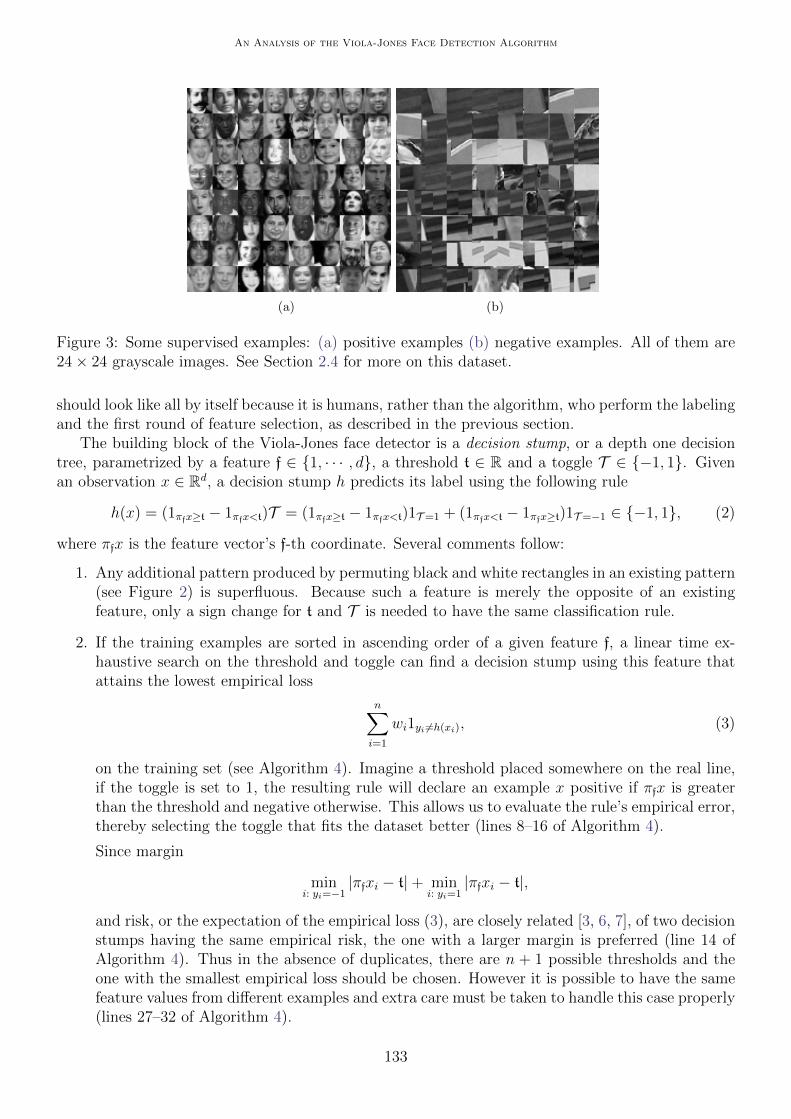
Figure 3: Some supervised examples: (a) positive examples (b) negative examples. All of them are24× 24 grayscale images. See Section 2.4 for more on this dataset.

should look like all by itself because it is humans, rather than the algorithm, who perform the labelingand the first round of feature selection, as described in the previous section.

The building block of the Viola-Jones face detector is a decision stump, or a depth one decisiontree, parametrized by a feature f ∈ {1, · · · , d}, a threshold t ∈ R and a toggle T ∈ {−1, 1}. Givenan observation x ∈ Rd, a decision stump h predicts its label using the following rule

h(x) = (1πfx≥t − 1πfx<t)T = (1πfx≥t − 1πfx<t)1T =1 + (1πfx<t − 1πfx≥t)1T =−1 ∈ {−1, 1}, (2)

where πfx is the feature vector’s f-th coordinate. Several comments follow:

1. Any additional pattern produced by permuting black and white rectangles in an existing pattern(see Figure 2) is superfluous. Because such a feature is merely the opposite of an existingfeature, only a sign change for t and T is needed to have the same classification rule.

2. If the training examples are sorted in ascending order of a given feature f, a linear time ex-haustive search on the threshold and toggle can find a decision stump using this feature thatattains the lowest empirical loss

n∑i=1

wi1yi 6=h(xi), (3)

on the training set (see Algorithm 4). Imagine a threshold placed somewhere on the real line,if the toggle is set to 1, the resulting rule will declare an example x positive if πfx is greaterthan the threshold and negative otherwise. This allows us to evaluate the rule’s empirical error,thereby selecting the toggle that fits the dataset better (lines 8–16 of Algorithm 4).

Since margin

mini: yi=−1

|πfxi − t|+ mini: yi=1

|πfxi − t|,

and risk, or the expectation of the empirical loss (3), are closely related [3, 6, 7], of two decisionstumps having the same empirical risk, the one with a larger margin is preferred (line 14 ofAlgorithm 4). Thus in the absence of duplicates, there are n + 1 possible thresholds and theone with the smallest empirical loss should be chosen. However it is possible to have the samefeature values from different examples and extra care must be taken to handle this case properly(lines 27–32 of Algorithm 4).

133

Yi-Qing Wang

Algorithm 4 Decision Stump by Exhaustive Search

1: Input: n training examples arranged in ascending order of feature πfxi: πfxi1 ≤ πfxi2 ≤ · · · ≤πfxin , probabilistic example weights (wk)1≤k≤n.

2: Output: the decision stump’s threshold τ , toggle T , error E and margin M.3: Initialization: τ ← min1≤i≤n πfxi − 1, M ← 0 and E ← 2 (an arbitrary upper bound of the

empirical loss).4: Sum up the weights of the positive (resp. negative) examples whose f-th feature is bigger than

the present threshold: W+1 ←

∑ni=1wi1yi=1 (resp. W+

−1 ←∑n

i=1wi1yi=−1).5: Sum up the weights of the positive (resp. negative) examples whose f-th feature is smaller than

the present threshold: W−1 ← 0 (resp. W−

−1 ← 0).

6: Set iterator j ← 0, τ ← τ and M ←M.7: while true do8: Select the toggle to minimize the weighted error: error+ ← W−

1 +W+−1 and error− ← W+

1 +W−−1.

9: if error+ < error− then10: E ← error+ and T ← 1.11: else12: E ← error− and T ← −1.13: end if14: if E < E or E = E & M >M then15: E ← E , τ ← τ , M← M and T ← T .16: end if17: if j = n then18: Break.19: end if20: j ← j + 1.21: while true do22: if yij = −1 then23: W−

−1 ← W−−1 + wij and W+

−1 ← W+−1 − wij .

24: else25: W−

1 ← W−1 + wij and W+

1 ← W+1 − wij .

26: end if27: To find a new valid threshold, we need to handle duplicate features.28: if j = n or πfxij 6= πfxij+1

then29: Break.30: else31: j ← j + 1.32: end if33: end while34: if j = n then35: τ ← max1≤i≤n πfxi + 1 and M ← 0.36: else37: τ ← (πfxij + πfxij+1

)/2 and M ← πfxij+1− πfxij .

38: end if39: end while

134

An Analysis of the Viola-Jones Face Detection Algorithm

Algorithm 5 Best Stump

1: Input: n training examples, their probabilistic weights (wi)1≤i≤n, number of features d.2: Output: the best decision stump’s threshold, toggle, error and margin.3: Set the best decision stump’s error to 2.4: for f = 1 to d do5: Compute the decision stump associated with feature f using Algorithm 4.6: if this decision stump has a lower weighted error (3) than the best stump or a wider margin

if the weighted error are the same then7: set this decision stump to be the best.8: end if9: end for

Algorithm 6 Adaboost

1: Input: n training examples (xi, yi) ∈ Rd × {−1, 1}, 1 ≤ i ≤ n, number of training rounds T .2: Parameter: the initial probabilistic weights wi(1) for 1 ≤ i ≤ n.3: Output: a strong learner/committee.4: for t = 1 to T do5: Run Algorithm 5 to train a decision stump ht using the weights w·(t) and get its weighted

error εt

εt =n∑i=1

wi(t)1ht(xi)6=yi ,

6: if εt = 0 and t = 1 then7: training ends and return h1(·).8: else9: set αt = 1

2ln(1−εt

εt).

10: update the weights

∀i, wi(t+ 1) =wi(t)

2

( 1

εt1ht(xi)6=yi +

1

1− εt1ht(xi)=yi

).

11: end if12: end for13: Return the rule

fT (·) = sign[ T∑t=1

αtht(·)].

135

Yi-Qing Wang

By adjusting individual example weights (Algorithm 6 line 10), Adaboost makes more effort tolearn harder examples and adds more decision stumps (see Algorithm 5) in the process. Intuitively,in the final voting, a stump ht with lower empirical loss is rewarded with a bigger say (a higherαt, see Algorithm 6 line 9) when a T -member committee (vote-based classifier) assigns an exampleaccording to

fT (·) = sign[ T∑t=1

αtht(·)].

How the training examples should be weighed is explained in detail in Appendix A. Figure 4 showsan instance where Adaboost reduces false positive and false negative rates simultaneously as moreand more stumps are added to the committee. For notational simplicity, we denote the empiricalloss by

n∑i=1

wi(1)1yi∑T

t=1 αtht(xi)≤0 := P(fT (X) 6= Y ),

where (X, Y ) is a random couple distributed according to the probability P defined by the weightswi(1), 1 ≤ i ≤ n set when the training starts. As the empirical loss goes to zero with T , so do bothfalse positive P(fT (X) = 1|Y = −1) and false negative rates P(fT (X) = −1|Y = 1) owing to

P(fT (X) 6= Y ) = P(Y = 1)P(fT (X) = −1|Y = 1) + P(Y = −1)P(fT (X) = 1|Y = −1).

Thus the detection rate

P(fT (X) = 1|Y = 1) = 1− P(fT (X) = −1|Y = 1),

must tend to 1.Thus the size T of the trained committee depends on the targeted false positive and false negative

rates. In addition, let us mention that, given n− negative and n+ positive examples in a trainingpool, it is customary to give a negative (resp. positive) example an initial weight equal to 0.5/n−(resp. 0.5/n+) so that Adaboost does not favor either category at the beginning.

2.3 Attentional Cascade

In theory, Adaboost can produce a single committee of decision stumps that generalizes well. How-ever, to achieve that, an enormous negative training set is needed at the outset to gather all possiblenegative patterns. In addition, a single committee implies that all the windows inside an image haveto go through the same lengthy decision process. There has to be another more cost-efficient way.

The prior probability for a face to appear in an image bears little relevance to the presentedclassifier construction because it requires both the empirical false negative and false positive rate toapproach zero. However, our own experience tells us that in an image, a rather limited number ofsub-windows deserve more attention than others. This is true even for face-intensive group photos.Hence the idea of a multi-layer attentional cascade which embodies a principle akin to that of Shannoncoding: the algorithm should deploy more resources to work on those windows more likely to containa face while spending as little effort as possible on the rest.

Each layer in the attentional cascade is expected to meet a training target expressed in falsepositive and false negative rates: among n negative examples declared positive by all of its precedinglayers, layer l ought to recognize at least (1− γl)n as negative and meanwhile try not to sacrifice itsperformance on the positives: the detection rate should be maintained above 1− βl.

136

An Analysis of the Viola-Jones Face Detection Algorithm

(a) (b)

Figure 4: Algorithm 6 ran with equally weighted 2500 positive and 2500 negative examples. Figure(a) shows that the empirical risk and its upper bound, interpreted as the exponential loss (seeAppendix A), decrease steadily over iterations. This implies that false positive and false negativerates must also decrease, as observed in (b).

At the end of the day, only the generalization error counts which unfortunately can only beestimated with some validation examples that Adaboost is not allowed to see at the training phase.Hence in Algorithm 10 at line 10, a conservative choice is made as to how one assesses the error rates:the higher false positive rate obtained from training and validation is used to evaluate how well thealgorithm has learned to distinguish faces from non-faces. The false negative rate is assessed in thesame way.

It should be kept in mind that Adaboost by itself does not favor either error rate: it aims toreduce both simultaneously rather than one at the expense of the other. To allow flexibility, oneadditional control s ∈ [−1, 1] is introduced to shift the classifier

fTs (·) = sign[ T∑t=1

αt(ht(·) + s

)], (4)

so that a strictly positive s makes the classifier more inclined to predict a face and vice versa.To enforce an efficient resource allocation, the committee size should be small in the first few

layers and then grow gradually so that a large number of easy negative patterns can be eliminatedwith little computational effort (see Figure 5).

Appending a layer to the cascade means that the algorithm has learned to reject a few newnegative patterns previously viewed as difficult, all the while keeping more or less the same positivetraining pool. To build the next layer, more negative examples are thus required to make the trainingprocess meaningful. To replace the detected negatives, we run the cascade on a large set of grayimages with no human face and collect their false positive windows. The same procedure is used forconstructing and replenishing the validation set (see Algorithm 7). Since only 24×24 sized examplescan be used in the training phase, those bigger false positives are down-sampled (Algorithm 8) andrecycled using Algorithm 9.

Assume that at layer l, a committee of Tl weak classifiers is formed along with a shift s so that theclassifier’s performance on training and validation set can be measured. Let us denote the achievedfalse positive and false negative rate by γl and βl. Depending on their relation with the targets γland βl, four cases are presented:

1. If the layer training target is fulfilled (Algorithm 10 line 11: γl ≤ γl and βl ≤ βl), the algorithmmoves on to training the next layer if necessary.

137

Yi-Qing Wang

Algorithm 7 Detecting faces with an Adaboost trained cascade classifier

1: Input: an M × N grayscale image I and an L-layer cascade of shifted classifiers trained usingAlgorithm 10

2: Parameter: a window scale multiplier c3: Output: P , the set of windows declared positive by the cascade4: Set P = {[i, i+ e− 1]× [j, j + e− 1] ⊂ I : e = J24cκK, κ ∈ N}5: for l = 1 to L do6: for every window in P do7: Remove the windowed image’s mean and compute its standard deviation.8: if the standard deviation is bigger than 1 then9: divide the image by this standard deviation and compute its features required by the

shifted classifier at layer l with Algorithm 310: if the cascade’s l-th layer predicts negative then11: discard this window from P12: end if13: else14: discard this window from P15: end if16: end for17: end for18: Return P

Algorithm 8 Downsampling a square image

1: Input: an e× e image I (e > 24)2: Output: a downsampled image O of dimension 24× 243: Blur I using a Gaussian kernel with standard deviation σ = 0.6

√( e24

)2 − 14: Allocate a matrix O of dimension 24× 245: for i = 0 to 23 do6: for j = 0 to 23 do7: Compute the scaled coordinates i← e−1

25(i+ 1), j ← e−1

25(j + 1)

8: Set imax ← min(JiK + 1, e − 1), imin ← max(0, JiK), jmax ← min(JjK + 1, e − 1), jmin ←max(0, JjK)

9: Set O(i, j) = 14

[I (imax, jmax) + I (imin, jmax) + I (imin, jmin) + I (imax, jmin)

]10: end for11: end for12: Return O

138

An Analysis of the Viola-Jones Face Detection Algorithm

Algorithm 9 Collecting false positive examples for training a cascade’s (L+ 1)-th layer

1: Input: a set of grayscale images with no human faces and an L-layer cascade of shifted classifiers

2: Parameter: a window scale multiplier c3: Output: a set of false positive examples V4: for every grayscale image do5: Run Algorithm 7 to get all of its false positives Q6: for every windowed image in Q do7: if the window size is bigger than 24× 24 then8: downsample this subimage using Algorithm 8 and run Algorithm 7 on it9: if the downsampled image remains positive then

10: accept this false positive to V11: end if12: else13: accept this false positive to V14: end if15: end for16: end for17: Return V

2. If there is room to improve the detection rate (Algorithm 10 line 13: γl ≤ γl and βl > βl), s isincreased by u, a prefixed unit.

3. If there is room to improve the false positive rate (Algorithm 10 line 20: γl > γl and βl ≤ βl),s is decreased by u.

4. If both error rates fall short of the target (Algorithm 10 line 27: γl > γl and βl > βl), thealgorithm, if the current committee does not exceed a prefixed layer specific size limit, trainsone more member to add to the committee.

Special attention should be paid here: the algorithm could alternate between case 2 and 3 and createa dead loop. A solution is to halve the unit u every time it happens until u becomes smaller than10−5. When it happens, one more round of training at this layer is recommended.

As mentioned earlier, to prevent a committee from growing too big, the algorithm stops refiningits associated layer after a layer dependent size limit is breached (Algorithm 10 line 28). In this case,the shift s is set to the smallest value that satisfies the false negative requirement. A harder learningcase is thus deferred to the next layer. This strategy works because Adaboost’s inability to meetthe training target can often be explained by the fact that a classifier trained on a limited numberof examples might not generalize well on the validation set. However, those hard negative patternsshould ultimately appear and be learned if the training goes on, albeit one bit at a time.

To analyze how well the cascade does, let us assume that at layer l, Adaboost can deliver aclassifier fTll,sl with false positive γl and detection rate 1− βl. In probabilistic terms, it means

P(fTll,sl(X) = 1|Y = 1) ≥ 1− βl and P(fTll,sl(X) = 1|Y = −1) ≤ γl,

where by abuse of notation we keep P to denote the probability on some image space. If Algorithm 10halts at the end of L iterations, the decision rule is

fcascade(X) = 2( L∏l=1

1fTll,sl

(X)=1− 1

2

).

139

Yi-Qing Wang

Algorithm 10 Attentional Cascade1: Input: n training positives, m validation positives, two sets of gray images with no human faces to

draw training and validation negatives, desired overall false positive rate γo, and targeted layer falsepositive and detection rate γl and 1− βl.

2: Parameter: maximum committee size at layer l: Nl = min(10l + 10, 200).3: Output: a cascade of committees.4: Set the attained overall false positive rate γo ← 1 and layer count l← 0.5: Randomly draw 10n negative training examples and m negative validation examples.6: while γo > γo do7: u← 10−2, l← l + 1, sl ← 0, and Tl ← 1.8: Run Algorithm 6 on the training set to produce a classifier fTll = sign

[∑Tlt=1 αtht

].

9: Run the sl-shifted classifier fTll,sl = sign[∑Tl

t=1 αt(ht + sl

)], on both the training and validation set to

obtain the empirical and generalized false positive (resp. false negative) rate γe and γg (resp. βe andβg).

10: γl ← max(γe, γg) and βl ← max(βe, βg).

11: if γl ≤ γl and 1− βl ≥ 1− βl then12: γo ← γo × γl.13: else if γl ≤ γl, 1− βl < 1− βl and u > 10−5 (there is room to improve the detection rate) then14: sl ← sl + u.15: if the trajectory of sl is not monotone then16: u← u/2.17: sl ← sl − u.18: end if19: Go to line 9.20: else if γl > γl, 1− βl ≥ 1− βl and u > 10−5 (there is room to improve the false positive rate) then21: sl ← sl − u.22: if the trajectory of sl is not monotone then23: u← u/2.24: sl ← sl + u.25: end if26: Go to line 9.27: else28: if Tl > Nl then29: sl ← −130: while 1− βl < 0.99 do31: Run line 9 and 10.32: end while33: γo ← γo × γl.34: else35: Tl ← Tl + 1 (Train one more member to add to the committee.)36: Go to line 8.37: end if38: end if39: Remove the false negatives and true negatives detected by the current cascade

fcascade(X) = 2( l∏p=1

1fTpp,sp (X)=1

− 1

2

).

Use this cascade with Algorithm 9 to draw some false positives so that there are n training negativesand m validation negatives for the next round.

40: end while

41: Return the cascade.

140

An Analysis of the Viola-Jones Face Detection Algorithm

A window is thus declared positive if and only if all its component layers hold the same opinion

P(fcascade(X) = 1|Y = −1)

=P(L⋂l=1

{fTll,sl(X) = 1}|Y = −1)

=P(fTLL,sL(X) = 1|L−1⋂l=1

{fTll,sl(X) = 1} and Y = −1)P(L−1⋂l=1

{fTll,sl(X) = 1}|Y = −1)

≤γlP(L−1⋂l=1

{fTll,sl(X) = 1}|Y = −1)

≤γLl .

Likewise, the overall detection rate can be estimated as follows

P(fcascade(X) = 1|Y = 1)

=P(L⋂l=1

{fTll,sl(X) = 1}|Y = 1)

=P(fTLL,sL(X) = 1|L−1⋂l=1

{fTll,sl(X) = 1} and Y = 1)P(L−1⋂l=1

{fTll,sl(X) = 1}|Y = 1)

≥(1− βl)P(L−1⋂l=1

{fTll,sl(X) = 1}|Y = 1)

≥(1− βl)L.

In other words, if the empirically obtained rates are any indication, a faceless window will have aprobability higher than 1−γl to be labeled as such at each layer, which effectively directs the cascadeclassifier’s attention on those more likely to have a face (see Figure 6).

2.4 Dataset and Experiments

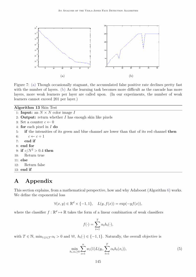
A few words on the actual cascade training carried out on a 8-core Linux machine with 48G memory.We first downloaded 2897 different images without human faces from [4, 9, 5], National Oceanic andAtmospheric Administration (NOAA) Photo Library2 and European Southern Observatory3. Theywere divided into two sets containing 2451 and 446 images respectively for training and validation.1000 training and 1000 validation positive examples from an online source4 were used. The trainingprocess lasted for around 24 hours before producing a 31-layer cascade. It took this long because itbecame harder to get 2000 false positives (1000 for training and 1000 for validation) using Algorithm 9with a more discriminative cascade: the algorithm needed to examine more images before it couldcome across enough good examples. The targeted false positive and false negative rate for each layerwere set to 0.5 and 0.995 respectively and Figure 7 shows how the accumulated false positive rate asdefined at line 12 and 33 of Algorithm 10 evolves together with the committee size. The fact thatthe later layers required more intensive training also contributed to a long training phase.

2http://www.photolib.noaa.gov/3http://www.eso.org/public/images/4http://www.cs.wustl.edu/~pless/559/Projects/faceProject.html

141

Yi-Qing Wang

(a) (b) (c) (d) (e) (f)

(g) (h) (i) (j) (k) (l)

(m) (n) (o) (p) (q) (r)

(s) (t) (u) (v) (w) (x)

Figure 5: A selection of negative training examples at round 21 (a) (b) (c) (d) (e) (f), round 26 (g)(h) (i) (j) (k) (l), round 27 (m) (n) (o) (p) (q) (r), round 28 (s) (t) (u) (v) (w) (x). Observe how thenegative training examples become increasingly difficult to discriminate from real faces.

3 Post-Processing

Figure 6(d) and Figure 8(a) show that the same face can be detected multiple times by a correctlytrained cascade. This should come as no surprise as the positive examples (see Figure 3(a)) doallow a certain flexibility in pose and expression. On the contrary, many false positives do not enjoythis stability, despite the fact that taken out of context, some of them do look like a face (also seeFigure 5). This observation lends support to the following detection confidence based heuristics forfurther reducing false positives and cleaning up the detected result (see Algorithm 11):

1. A detected window contains a face if and only if a sufficient number of other adjacent detectedwindows of the same size confirm it. To require windows of exactly the same size is not stringentbecause the test window sizes are quantified (see Algorithm 7 line 2). In this implementation,the window size multiplier is 1.5. Two e×e detected windows are said to be adjacent if and onlyif between the upper left corners of these two windows there is a path formed by the upper leftcorners of some detected windows of the same size. This condition is easily checked with theconnected component algorithm5 [8]. The number of test windows detecting a face is presumedto grow linearly with its size. This suggests the quotient of the cardinality of a connectedcomponent of adjacent windows by their common size e as an adequate confidence measure.

5We obtained a version from http://alumni.media.mit.edu/~rahimi/connected/.

142

An Analysis of the Viola-Jones Face Detection Algorithm

(a) (b)

(c) (d)

Figure 6: How the trained cascade performs with (a) 16 layers, (b) 21 layers, (c) 26 layers and (d)31 layers: the more layers, the less false positives.

This quotient is then compared to the scale invariant threshold empirically set at 3/24, whichmeans that to confirm the detection of a face of size 24× 24, three adjacent detected windowsare sufficient.

2. It is possible for the remaining detected windows to overlap after the previous test. In thiscase, we distinguish two scenarios (Algorithm 11 line 15–25):

(a) If the smaller window’s center is outside the bigger one, keep both.

(b) Keep the one with higher detection confidence otherwise.

Finally, to make the detector slightly more rotation-invariant, in this implementation, we de-cided to run Algorithm 7 three times, once on the input image, once on a clockwise rotated imageand once on an anti-clockwise rotated image before post-processing all the detected windows (seeAlgorithm 12). In addition, when available, color also conveys valuable information to help furthereliminate false positives. Hence in the current implementation, after the robustness test, an op-tion is offered as to whether color images should be post-processed with this additional step (seeAlgorithm 13). If so, a detected window is declared positive only if it passes both tests.

143

Yi-Qing Wang

Algorithm 11 Post-Processing

1: Input: a set G windows declared positive on an M ×N grayscale image2: Parameter: minimum detection confidence threshold r3: Output: a reduced set of positive windows P4: Create an M ×N matrix E filled with zeros.5: for each window w ∈ G do6: Take w’s upper left corner coordinates (i, j) and its size e and set E(i, j)← e7: end for8: Run a connected component algorithm on E.9: for each component C formed by |C| detected windows of dimension eC × eC do

10: if its detection confidence |C|e−1C > r then11: send one representing window to P12: end if13: end for14: Sort the elements in P in ascending order of window size.15: for window i = 1 to |P| do16: for window j = i+ 1 to |P| do17: if window j remains in P and the center of window i is inside of window j then18: if window i has a higher detection confidence than window j then19: remove window j from P20: else21: remove window i from P and break from the inner loop22: end if23: end if24: end for25: end for26: Return P .

Algorithm 12 Face detection with image rotation

1: Input: an M ×N grayscale image I2: Parameter: rotation θ3: Output: a set of detected windows P4: Rotate the image about its center by θ and −θ to have Iθ and I−θ5: Run Algorithm 7 on I, Iθ and I−θ to obtain three detected window sets P , Pθ and P−θ respectively

6: for each detected window w in Pθ do7: Get w’s upper left corner’s coordinates (iw, jw) and its size ew8: Rotate (iw, jw) about Iθ’s center by −θ to get (iw, jw)9: Quantify the new coordinates iw ← min(max(0, JiwK),M − 1) and jw ←

min(max(0, JjwK), N − 1)10: if there is no ew × ew window located at (iw, jw) in P then11: Add it to P12: end if13: end for14: Replace θ by −θ and go through lines 6–13 again15: Return P

144

An Analysis of the Viola-Jones Face Detection Algorithm

(a) (b)

Figure 7: (a) Though occasionally stagnant, the accumulated false positive rate declines pretty fastwith the number of layers. (b) As the learning task becomes more difficult as the cascade has morelayers, more weak learners per layer are called upon. (In our experiments, the number of weaklearners cannot exceed 201 per layer.)

Algorithm 13 Skin Test

1: Input: an N ×N color image I2: Output: return whether I has enough skin like pixels3: Set a counter c← 04: for each pixel in I do5: if the intensities of its green and blue channel are lower than that of its red channel then6: c← c+ 17: end if8: end for9: if c/N2 > 0.4 then

10: Return true11: else12: Return false13: end if

A Appendix

This section explains, from a mathematical perspective, how and why Adaboost (Algorithm 6) works.We define the exponential loss

∀(x, y) ∈ Rd × {−1, 1}, L(y, f(x)) = exp(−yf(x)),

where the classifier f : Rd 7→ R takes the form of a linear combination of weak classifiers

f(·) =T∑t=1

αtht(·),

with T ∈ N, min1≤t≤T αt > 0 and ∀t, ht(·) ∈ {−1, 1}. Naturally, the overall objective is

minht,αt≥0

n∑i=1

wi(1)L(yi,T∑t=1

αtht(xi)), (5)

145

Yi-Qing Wang

(a)

(b)

Figure 8: The suggested post-processing procedure further eliminates a number of false positives andbeautifies the detected result using a 31 layer cascade.

with some initial probabilistic weight wi(1). A greedy approach is deployed to deduce the optimalclassifiers ht and weights αt one after another, although there is no guarantee that the objective (5)is minimized. Given (αs, hs)1≤s<t, let Zt+1 be the weighted exponential loss attained by a t-membercommittee and we seek to minimize it through (ht, αt)

Zt+1 := minht,αt≥0

n∑i=1

wi(1)e−yi∑t

s=1 αshs(xi)

146

An Analysis of the Viola-Jones Face Detection Algorithm

= minht,αt≥0

n∑i=1

Di(t)e−αtyiht(xi)

= minht,αt≥0

n∑i=1

Di(t)e−αt1yiht(xi)=1 +

n∑i=1

Di(t)eαt1yiht(xi)=−1

= minht,αt≥0

e−αt

n∑i=1

Di(t) + (eαt − e−αt)n∑i=1

Di(t)1yiht(xi)=−1

=Zt minht,αt≥0

e−αt + (eαt − e−αt)n∑i=1

Di(t)

Zt1yiht(xi)=−1,

Therefore the optimization of Zt+1 can be carried out in two stages: first, because of αt’s assumedpositivity, we minimize the weighted error using a base learning algorithm, a decision stump forinstance

εt := minhZ−1t

n∑i=1

Di(t)1yih(xi)=−1,

ht := argminh

Z−1t

n∑i=1

Di(t)1yih(xi)=−1.

In case of multiple minimizers, take ht to be any of them. Next choose

αt =1

2ln

1− εtεt

= argminα>0

e−α + (eα − e−α)εt.

Hence εt < 0.5 is necessary, which imposes a minimal condition on the training set and the baselearning algorithm. Also obtained is

Zt+1 = 2Zt√εt(1− εt) ≤ Zt,

a recursive relation asserting the decreasing behavior of the exponential risk. Weight change thusdepends on whether an observation is misclassified

wi(t+ 1) =Di(t+ 1)

Zt+1

=Di(t)e

−yiαtht(xi)

2Zt√εt(1− εt)

=wi(t)

2

(1ht(xi)=yi

1

1− εt+ 1ht(xi) 6=yi

1

εt

).

The final boosted classifier is thus a weighted committee

f(·) := sign[ T∑t=1

αtht(·)].

Acknowledgements

Research partially financed by the European Research Council, advanced grant “Twelve labours”,the Office of Naval research under grant N00014-97-1-0839, and by DxO labs.

147

Yi-Qing Wang

Image Credits

by The Heart Truth, Flickr6 CC-BY-SA-2.0.

The USC-SIPI7 Image Database.

References

[1] Y. Freund and R. Schapire, A decision-theoretic generalization of on-line learning andan application to boosting, Journal of Computer and System Sciences, 55 (1997), pp. 119–139.http://dx.doi.org/10.1006/jcss.1997.1504.

[2] Y. Freund, R. Schapire, and N. Abe, A short introduction to boosting, Journal of JapaneseSociety For Artificial Intelligence, 14 (1999), pp. 771–780.

[3] J. Friedman, T. Hastie, and R. Tibshirani, The Elements of Statistical Learning, vol. 1,Springer Series in Statistics, 2001.

[4] H. Jegou, M. Douze, and C. Schmid, Hamming embedding and weak geometric consistencyfor large scale image search, in European Conference on Computer Vision, vol. I of LectureNotes in Computer Science, Springer, 2008, pp. 304–317.

[5] A. Olmos, A biologically inspired algorithm for the recovery of shading and reflectance images.,Perception, 33 (2004), pp. 1463–1473. http://dx.doi.org/10.1068/p5321.

[6] F. Rosenblatt, The perceptron: a probabilistic model for information storage and organizationin the brain., Psychological review, 65 (1958), pp. 386–408. http://dx.doi.org/10.1037/

h0042519.

[7] R. E. Schapire, Y. Freund, P. Bartlett, and W. S. Lee, Boosting the margin: Anew explanation for the effectiveness of voting methods, The Annals of Statistics, 26 (1998),pp. 1651–1686. http://dx.doi.org/10.1214/aos/1024691352.

[8] L. Shapiro and G.C. Stockman, Computer vision, 2001. ISBN 0130307963.

[9] G. Tkacik, P. Garrigan, C. Ratliff, G. Milcinski, J. M. Klein, L. H. Seyfarth,P. Sterling, D. H. Brainard, and V. Balasubramanian, Natural images from the birth-place of the human eye, Public Library of Science One, 6 (2011), p. e20409.

[10] P. Viola and M. J. Jones, Robust real-time face detection, International Journal of ComputerVision, 57 (2004), pp. 137–154. http://dx.doi.org/10.1023/B:VISI.0000013087.49260.fb.

6http://www.flickr.com/photos/thehearttruth/3281640031/in/photostream/7http://sipi.usc.edu/database/

148