An Analysis of Radial Basis Functions and

Application in 2D Edge Detection

Tania OliveiraUndergraduate Student

Dept. of MathematicsUMass Dartmouth, Dartmouth MA 02747

Email: toliveira@umassd.edu

August 4, 2010

Abstract

The following is a study of radial basis functions (RBFs) and their role in approximatingone-dimensional graphs, and how this approach successfully extends to detecting edges in two-dimensional images. Multi-quadric, inverse multi-quadric, and Gaussian RBFs were tested inapproximating one-dimensional function graphs (both continuous and discontinuous) for dif-ferent shape parameters and interpolation point scales. A multi-quadric RBF was utilized ina Matlab program, generated by an advising professor, to calculate spatial relations of pointswithin a given image and interpolate intermediary points. The output of this program producesan edge map of the original image on a black and white coordinate matrix. An increased ep-silon value has been noted to heighten sensitivity to noise found in less defined image contrastsprocessed by this program.

1 Introduction

Upon entering the CSUMS program at UMass Dartmouth in the summer of 2010, Professor Gottliebpresented me with a research topic dealing with radial basis functions (RBFs) and their applicationto a successfully operating two-dimensional edge-detection program prepared in MatLab by herselfand a co-researcher in the field, Jae-Hun Jung. At the beginning of this project, I was provided withthe aforementioned program so that I could use it to process different images and examine the edgemaps produced when testing the effect of different values for parameters such as tmp = linspace(””,” ”,N) (interpolate density) and epsilon (shape parameter) within the code. Upon analyzing thecode, I learned that the program used a multi-quadric (MQ) RBF to calculate and interpolate pointsfrom the x-direction and y-direction, respectively, then overlapped these two approximated pointmaps over each other in the final product edge map matrix.

In order to better understand RBFs and their role in approximation, I generated a code usingMatLab to plot given one-dimensional functions in juxtaposition with their MQ RBF approximationplots in the same domain for escalating numbers of center-points. As the number of center-pointsincreased, the MQ RBF approximation more closely converged with the actual function, as expected,since the center-points are the points where the RBF values and actual function values matchperfectly or at least, as closely as the machine’s maximum rounding error will allow.

As the project progressed, I started to investigate two other RBF methods in addition to theMQ RBF. Based upon my previous code, I created another MatLab program which plotted a givenfunction along with its multi-quadric, inverse multi-quadric, and Gaussian RBF approximations foruniform conditions. Then, I began to analyze how the scale of interpolation points to the numberof center-points and the value of the shape parameter, epsilon, influenced the behavior of each ofthese RBF methods in approximating both continuous and discontinuous functions. Also, I tooknote of the average amount of error incurred by each of the three RBF methods and which of theseproduced more stable and accurate graphs that better matched the original function.

1

2 What are Radial Basis Functions?

Radial basis functions are functions which use the relationship of radial distances between designatedpoints on a given function, called center-points, and a special matrix calculation to figure missinglambda (λ) coefficients to interpolate intermediary data points and create an estimate function whichideally fits the position and shape of the original function as accurately as possible.

The following is an example of a multi-quadric (MQ) RBF:

φj =√

(xi − xj)2 + ε2j

As you can see, the RBF function represented by phi, (φj), incorporates a calculation of distancebetween center-points i and j. Epsilon, (εj), is a shape parameter, which, in some cases can varydepending on center-point j, but in the proceeding tests and examples will remain a constant value.

s(xi) =

N∑j=1

λjφj(||xi − xj ||, εj) = f(xi)

The sum of the RBF calculations using distances between xi and center-points j, from 1 → N ,multiplied by j−corresponding lambda coefficients should equal the exact value of the given functionat point xi.

This concept may be extended to multiple function values for N center-points using an N x Nphi matrix and a lambda vector of unknown coefficients, which when multiplied together, shouldresult in the exact values of the function at those corresponding selected center-points:

φ(x1,j1) φ(x1,j2) · · · φ(x1,jN )

φ(x2,j1) φ(x2,j2) · · · φ(x2,jN )

......

. . ....

φ(xN ,j1) φ(xN ,j2) · · · φ(xN ,jN )

λ1λ2...λN

=

f(1)f(2)

...f(N)

(1)

Mλ = f

In order to derive the lambda coefficient values, a simple inverse matrix multiplication is per-formed.

λ1λ2...λN

=

φ(x1,j1) φ(x1,j2) · · · φ(x1,jN )

φ(x2,j1) φ(x2,j2) · · · φ(x2,jN )

......

. . ....

φ(xN ,j1) φ(xN ,j2) · · · φ(xN ,jN )

f(1)f(2)

...f(N)

(2)

λ = M−1f

2.1 Interpolation

By applying the lambda coefficients obtained from the previous process to a greater number ofcenter-points (Ny), one can interpolate, or approximate, the points in between the prior range ofcenter-points simply by multiplying the same coefficients. A greater number of center-points forinterpolation leads to the following matrix operation using an Ny x N phi matrix called My:

φ(x1,j1) φ(x1,j2) · · · φ(x1,jN )

φ(x2,j1) φ(x2,j2) · · · φ(x2,jN )

......

. . ....

......

. . ....

φ(xNy,j1) φ(xNy,j2) · · · φ(xNy,jN )

λ1λ2...λN

=

f(1)f(2)

...

...f(Ny)

(3)

Myλ = f

2

2.2 Jump Discontinuities/Gibb’s Phenomenon

Functions behave in different ways, they can either be smooth and continuous, or they can containbreaks or jumps, making them discontinuous. Considering the interpolation method which RBFapproximation uses to estimate given functions, errors as well as oscillations, referred to as Gibb’sphenomenon, may occur around the jump.

Here is an example of a smooth function, sin(x), approximated by a MQ RBF for 100 center-points:

And here is an example of a discontinuous step function, approximated by the same techniquefor the same number of center-points:

As you can tell, the blue oscillations near the vertical jumpline indicate where the MQ RBFis experiencing Gibb’s phenomenon. Some mathematicians who research RBFs often seek to findmethods of eliminating these oscillations in order to make the approximation more accurate. Inhis paper, Jung proposes methods of detecting local discontinuities such as by finding the firstderivatives of the function to determine any radical changes in slope, and examining the lambdacoefficient vectors to locate a value that deviates from the rest, then proceeding to adapt the epsilon(ε) shape parameter to correct any digressions from the actual function [1].

3

3 RBFs in Approximating 1D Function Graphs

To begin studying RBFs and their behavior, I created and used a MatLab program to plot givenfunctions and their RBF approximations as well as produce a graph demonstrating the averageerror at each centerpoint on the domain. First, I began with a MQ RBF for increasing numbers ofcenterpoints, while maintaining a constant interpolation factor of 2 and epsilon of 0.1. The followingis an example output of the program, plotting MQ RBF approximations from 5 → 20 center-points,for the given function, cos(x), as well as displaying approximation errors at the maximum numberof center-points:

In all the proceeding graph experiments, I set the default conditions to be the static values N*2for Ny (interpolation scale) and 0.1 for eps (shape parameter). Also, all RBF calculations wereperformed on sets of equidistant points.

3.1 Three RBF Methods

After preparing the previous MatLab program, I decided to code a new version of the program thatplotted a given function and its approximations by three different RBF techniques using the sameconditions. The three RBFs which I tested and compared were the following:√

(xi − xj)2 + ε2j

Multi-Quadric: (MQ)

1√(xi − xj)2 + ε2j

Inverse Multi-Quadric: (I)

e−ε2j (xi−xj)

2

Gaussian: (G)

In the next figures, I experimented with significantly increasing the interpolation scale (Ny) andshape parameter (eps) from the original defaults to see how these changes would affect the behaviorof each RBF method. The three RBF approximations are plotted simultaneously against the samefunctions, and in each graph, the functions are represented by the following color code: red -ActualFunction, blue-MQ RBF, black -I RBF, green-G RBF.

4

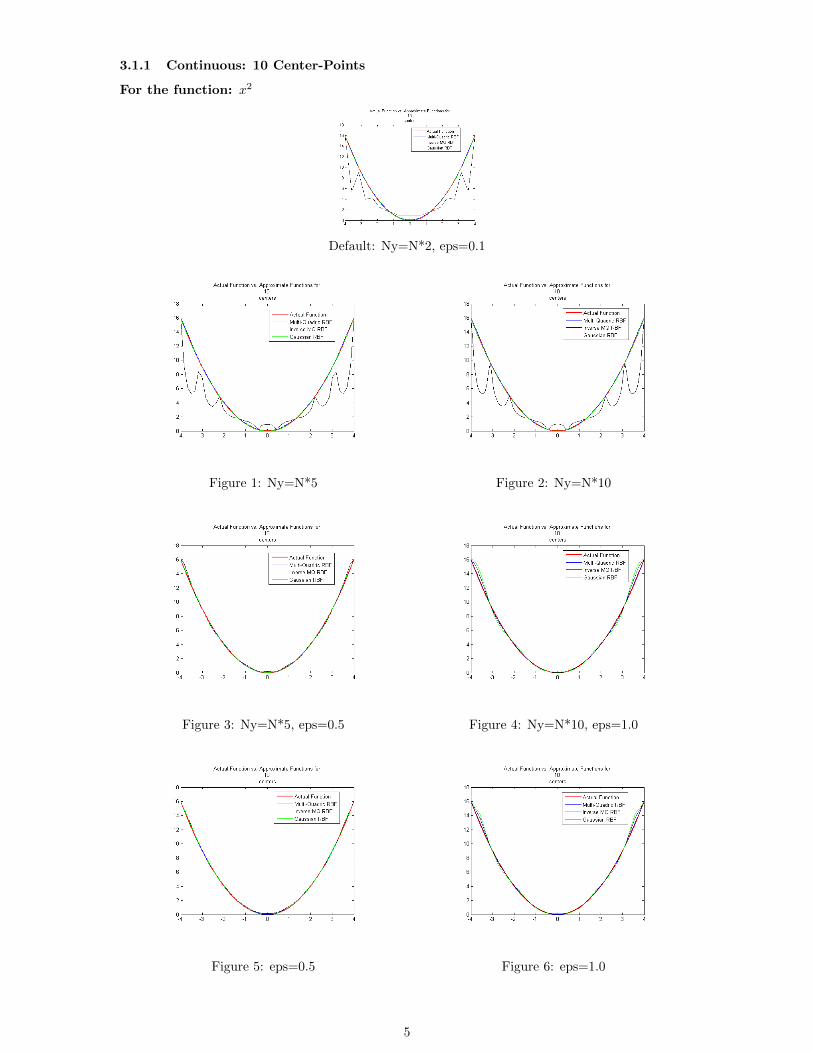
3.1.1 Continuous: 10 Center-Points

For the function: x2

Default: Ny=N*2, eps=0.1

Figure 1: Ny=N*5 Figure 2: Ny=N*10

Figure 3: Ny=N*5, eps=0.5 Figure 4: Ny=N*10, eps=1.0

Figure 5: eps=0.5 Figure 6: eps=1.0

5

3.1.2 Discontinuous: 10 Center-Points

For the function: f(x) = 1 when x > −3

Default: Ny=N*2, eps=0.1

Figure 7: Ny=N*5 Figure 8: Ny=N*10

Figure 9: Ny=N*5, eps=0.5 Figure 10: Ny=N*10, eps=1.0

Figure 11: eps=0.5 Figure 12: eps=1.0

6

3.1.3 Discontinuous: 100 Center-Points

For the function: |x|

Default: Ny=N*2, eps=0.1

Figure 13: Ny=N*5 Figure 14: Ny=N*10

Figure 15: Ny=N*5, eps=0.5 Figure 16: Ny=N*10, eps=1.0

Figure 17: eps=0.5 Figure 18: eps=1.0

7

3.1.4 1D Graph Observations

From the graph examples I collected, I noticed a particularly substantial effect in the behavior ofI RBF and G RBF when increasing the interpolation factor (Ny) and shape parameter (eps). Myreasoning behind using 10 and 100 center-points was to base these tests off a simple scale of pointsas well as to examine these behaviors at different extremes.

In the continuous 10 center-point case, the MQ RBF and G RBF smoothly fit to the shapeof the function, while the I RBF produced distant, jagged oscillations under default conditions.Incrementing the interpolation factor, however, worked to make this sharp oscillations more curvedand the centerpoints closer to the actual function as seen in Figure 1 and Figure 2. And increasingeps to 0.5 appeared to have produced the best fit of all the graph examples to the actual functionshape (See Figure 5), while increasing it further to 1.0 subjected the other RBF methods to worseapproximation (See Figure 6).

With the discontinuous 10 center-point case, the same change occurred in I RBF by increasingthe interpolation scale, but increasing epsilon had the same effect on all three RBF approximations.As epsilon was incremented, the area close to the jump discontinuity began to approach the verticalsteep more closely, while inducing waves and oscillations to incur along the rest of the line awayfrom the jump as demonstrated in Figures 9→12.

Finally, in the discontinous 100 center-point graph of |x|, it becomes clear that the G RBF methodradically oscillations and gives a very poor approximation for many equidistant center-points underthe default condition as well as under increased interpolation (See Figures 13 and 14). MQ RBFand I RBF approximations, however, seem to behave favorably given greater numbers of center-points. Although the erratic oscillations do not disappear, the incrementation of eps does help tomatch the G RBF estimation plot’s path onto that of the original function and the greater the eps,it seems, the closer the G approximations, up until eps=1, it seems (See Figures 15→18).

3.1.5 Error Comparisons

In all the graph tests I performed for these three RBFs, I discerned a trend in the error severity andthe graphical accuracy of each method. Overall, the MQ RBF was the most stable and consistentin approximating the actual shapes of the given functions while maintaining about a 10−15 amountof error at centerpoints, closely second to I RBF’s error accuracy by a very minute margin, so MQRBF appears to be the most reliable RBF approximation method. And G RBF always produced adrastically larger error than the other two methods in every case. The following is a sample errorplot for the function, sin(x), at 10 center-points:

8

4 Using MQ RBF in 2D Edge Detection

4.1 A Slice-by-Slice Approach

Upon reading through the 2D Edge Detection program written in MatLab, I noticed the the codesimply executes MQ RBF approximation in 1D from the x-direction, then from the y-direction, andlater overlaps these two 1D shock maps together to form the 2D edge map which illustrates theoriginal image’s edge locations.

2D Edge Maps

4.2 Changing linspace and epsilon

Utilizing the 2D edge detection code supplied me at the start of the project, I changed parameters,tmp = linspace(” ”,” ”,N) (interpolate density) and epsilon (shape parameter), to see how theseaffected the clarity of the edge maps.

Figure 19: linspace(-10,10,N), epsilon=0.1 Figure 20: linspace(-10,10,N), epsilon=0.2

Figure 21: linspace(-20,20,N), epsilon=0.1 Figure 22: linspace(-20,20,N), epsilon=0.2

9

4.3 Epsilon and Noise Detection

Following the observations made during interpolation and shape parameter tests in the 2D edgedetection code, I noticed a special effect of epsilon in improving noise detection within the image.In the edge maps below, the epsilon value was increased each time by 0.1 from values 0.5→ 0.9:

If you’ll notice, from left to right and down, as the shape parameter increases, the edges becomemore defined in the edge map, the 0.9 condition at the bottom being the clearest of all five testmaps. So, effectively, an increased shape parameter will allow for better noise detection, especiallyin soft contrasts, but exaggerating the shape parameter along with the interpolation density willmake for a very busy and noisy edge map, as seen in Figure 20.

5 Conclusion

From the results I collected, I’ve determined the interpolation scale and shape parameter dramati-cally affect the behavior of both I RBF and G RBF approximations, and that, at least for equidistantcenter-points, G RBFs are highly unstable for discontinuous functions, and this is very notable ina high degree of center-point evaluations. There may, however, exist procedures preemptive condi-tions to correct or prevent these inaccuracies. Overall, I found that MQ RBF was the most stableapproximation method with a relatively low degree of error at center-points. Therefore, making itthe optimal RBF method to use in the 2D edge detection code that was given to me at the beginningof the project.

In regards to 2D edge detection, I can deduce that RBFs can be successfully applied in performingadequate two-dimensional edge finding, using a simple 1D approach in both horizontal and vertical

10

directions. Also, an increased shape parameter serves to improve sensitivity to noise and loweraberrances in contrast in the images being processed.

6 Acknowledgements

For opening the door for me to join the CSUMS research group this summer, I would like to thankProf. Alfa Heryudono, because I wouldn’t have gotten involved in this work if it hadn’t been forhis initiative. I would like to thank Prof. Sigal Gottlieb for giving me this topic and the resourcesI needed to begin and I would also like to thank Prof. Saeja Kim for helping me learn exactly howRBFs operated so that I could enter the project with a better understanding of the material. I alsoappreciated the assistance that certain members of the CSUMS group offered me during the courseof the project: I would like to thank Sidafa Conde and Zachary Grant for helping me program inMatLab, Prof. Adam Hausknecht and T.A., Dan Higgs for their technical support, Prof. GaryDavis for his guidance and humor, and the rest of the CSUMS advisers and students for making thissuch a positive researching experience. Lastly, I would like to express thanks to the National ScienceFoundation for funding this research program and I hope they will continue to fund and show theirsupport for invaluable educational experiences like these in the future.

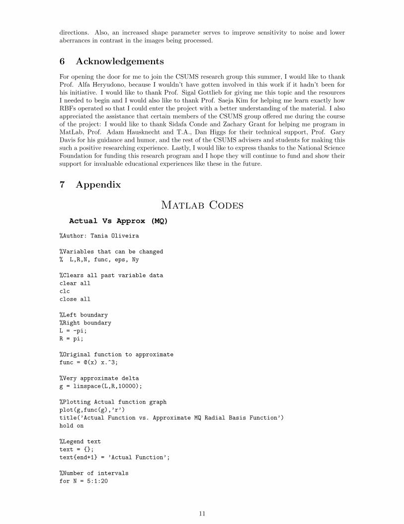
7 Appendix

Matlab Codes

Actual Vs Approx (MQ)

%Author: Tania Oliveira

%Variables that can be changed

% L,R,N, func, eps, Ny

%Clears all past variable data

clear all

clc

close all

%Left boundary

%Right boundary

L = -pi;

R = pi;

%Original function to approximate

func = @(x) x.^3;

%Very approximate delta

g = linspace(L,R,10000);

%Plotting Actual function graph

plot(g,func(g),’r’)

title(’Actual Function vs. Approximate MQ Radial Basis Function’)

hold on

%Legend text

text = {};

text{end+1} = ’Actual Function’;

%Number of intervals

for N = 5:1:20

11

text{end+1} = sprintf(’N = %i’, N);

%List of points on a specified range

x = linspace(L,R,N);

%Epsilon shape parameter

eps = 0.1;

%row elements and column elements of the phi matrix

r = 1;

c = 1;

%Phi function

phi = @(r,c) sqrt((r-c)^2+eps^2);

%Matrix of phi function values

%Need ’for’ loops to increment c across the row and r down the columns

M = [];

for r = 1:N

for c = 1:N

M(r,c) = phi(x(r),x(c));

end

end

%Matrix of original function values

f = func(x);

f = f(:); %transpose to vertical f vector

%Matrix of lambda coefficients

lambda = M\f;

lambda = lambda(:); %transpose to vertical lambda vector

F = M*lambda;

%~INTERPOLATION~

%Ny should be greater than N

Ny = N*2;

y = linspace(L,R,Ny);

My = [];

for r = 1:Ny

for c = 1:N

My(r,c) = phi(y(r),x(c));

end

end

Fy = My*lambda;

%Variable to randomize line color

clrd = [rand, rand, rand];

%Plotting Approximate functions

plot(y,Fy,’color’,clrd)

text = [text; ’N= ’, num2str(N)];

%pause(0.5)

end

12

legend(text)

%Plot Error of Approximation for Maximum Center-points

figure

semilogy(x,abs(F-f))

title(’Approximation Error’)

Actual Vs Approx 3 RBFs

%Author: Tania Oliveira

%Variables that can be changed

% L,R,func,N,eps,Ny

%Clears all past variable data

clear all

clc

close all

%Left boundary

%Right boundary

L = -4;

R = 4;

%%%%%%%%%%%%%%%%%%%%%%%%%%%%%%%%%%%%%%%%%%%%%%%%%%%%%%%%%%%%%%%%%%%%%%%%%%%

%Number of centers

N = 100;

%List of points on a specified range

x = linspace(L,R,N); %equidistant

%x = logspace(L,R,N);

%Epsilon shape parameter

eps = 0.1;

%%%%%%%%%%~INTERPOLATION~%%%%%%%%%%

%Number of interpolation centers (Ny should be greater than N)

Ny = N*2;

%List of interpolation points on a specified range

y = linspace(L,R,Ny);

%%%%%%%%%%%%%%%%%%%%%%%%%%%%%%%%%%%%%%%%%%%%%%%%%%%%%%%%%%%%%%%%%%%%%%%%%%%

%Very approximate delta

s = linspace(L,R,10000);

%func = @(s) log(s);

%func = @(s) sin(1./s);

%func = @(s) csc(s);

%func = @(s) tan(s);

%func = @(s) 1./(s-1);

%Piece-wise discontinuous function ex.

%func = @(s) (s+4).*(s < 0) + (6).*(s == 0) + (cos(s)).*(s > 0);

13

%func = @(s) (s.^2).*(s < -2) + (sqrt(s)).*(s > 2);

%func = @(s) 1.*(s < 0) - 1.*(s >= 0);

func = @(s) -1.*(s<0)+1.*(s>0);

%Plotting Actual function graph

plot(s,func(s),’r’,’LineWidth’,2)

titletext = {’Actual Function vs. Approximate Functions for’,num2str(N),’ centers’};

title(titletext)

hold on

text = {};

text{end+1} = ’Actual Function’;

%List of original function values

f = func(x);

%transpose to vertical matrix

f = f(:);

%>>>RBF Calculations Start

%%%%%%%%%%%%%%%%%%%%%%%%%%%%%%%%%%%%%%%%%%%%%%%%%%%%%%%%%%%%%%%%%%%%%%%%%%%

% [ [1] ] %

% Multi-Quadric RBF %

qRBF = @(r,c) sqrt((r-c)^2+eps^2);

%Matrix of qRBF (multi-quadric) function values

qM = [];

for r = 1:N

for c = 1:N

qM(r,c) = qRBF(x(r),x(c));

end

end

%Matrix of multi-quadric lambda coefficients

qlambda = qM\f;

qlambda = qlambda(:); %transpose to vertical lambda vector

qF = qM*qlambda;

%INTERPOLATION

qMy = [];

for r = 1:Ny

for c = 1:N

qMy(r,c) = qRBF(y(r),x(c));

end

end

qFy = qMy*qlambda;

%Plotting multi-quadric approximation graph

plot(y,qFy,’b’)

text{end+1} = ’Multi-Quadric RBF’;

%%%%%%%%%%%%%%%%%%%%%%%%%%%%%%%%%%%%%%%%%%%%%%%%%%%%%%%%%%%%%%%%%%%%%%%%%%%

14

% [ [2] ] %

% Inverse Multi-Quadric RBF %

iRBF = @(r,c) 1./(sqrt((r-c)^2+eps^2));

%Matrix of iRBF (inverse multi-quadric) function values

iM = [];

for r = 1:N

for c = 1:N

iM(r,c) = iRBF(x(r),x(c));

end

end

%Matrix of inverse multi-quadric lambda coefficients

ilambda = iM\f;

ilambda = ilambda(:); %transpose to vertical lambda vector

iF = iM*ilambda;

%INTERPOLATION

iMy = [];

for r = 1:Ny

for c = 1:N

iMy(r,c) = iRBF(y(r),x(c));

end

end

iFy = iMy*ilambda;

%Plotting inverse multi-quadric approximation graph

plot(y,iFy,’k’)

text{end+1} = ’Inverse MQ RBF’;

%%%%%%%%%%%%%%%%%%%%%%%%%%%%%%%%%%%%%%%%%%%%%%%%%%%%%%%%%%%%%%%%%%%%%%%%%%%

% [ [3] ] %

% Gaussian RBF %

gRBF = @(r,c) exp(-((eps.^2)*((r-c).^2)));

%Matrix of gRBF (Guassian) function values

gM = [];

for r = 1:N

for c = 1:N

gM(r,c) = gRBF(x(r),x(c));

end

end

%Matrix of Guassian lambda coefficients

glambda = gM\f;

glambda = glambda(:); %transpose to vertical lambda vector

gF = gM*glambda;

%INTERPOLATION

gMy = [];

15

for r = 1:Ny

for c = 1:N

gMy(r,c) = gRBF(y(r),x(c));

end

end

gFy = gMy*glambda;

%Plotting Gaussian approximation graph

plot(y,gFy,’g’)

text{end+1} = ’Gaussian RBF’;

legend(text)

%%%%%%%%%%%%%%%%%%%%%%%%%%%%%%%%%%%%%%%%%%%%%%%%%%%%%%%%%%%%%%%%%%%%%%%%%%%

%Plot approximation errors at center-points for each method

figure

qError = abs(qF-f);

iError = abs(iF-f);

gError = abs(gF-f);

semilogy(x,qError,’b’)

hold on

semilogy(x,iError,’k’)

semilogy(x,gError,’g’)

legend(’Multi-Quadric RBF Error’,’Inverse MQ RBF Error’,’Gaussian RBF Error’)

title(’Approximation Error at Centers’)

Get Edge

% Subroutine for one-dimensional edge detection

%

% WE assume the rectangular domain for now.

%

% Jae-Hun Jung, August, 2007

%

function [lam, eps, where] = Get_Edge (x,f, M_in, MD_in)

M = M_in; MD = MD_in;

N = max(size(x));

epsilon = 0.1;

eps = x*0 + epsilon;

where = x*0+0;

inx = 0; index_p = 0;

Residual = 1;

while Residual >= 10^-10 %%%%%%%%%%%%%%%%%%%%%%%%%%%%%%%%%%%%%%%%%%%%%%%%%%%%%%

inx = inx+1;

lam = M\f; fd = MD*lam;

16

if inx == 1

lam1 = 2*lam;

end

edg =(abs(fd).*abs(lam));

edg = edg/max(max(edg));

ref = 0.5; % the tolerance level for the edge detection that can be modified.

for ix = 1:N

if edg(ix) >= ref

where(ix) = 1;

eps(ix) = 0;

M(1:N,ix) = (abs(x - x(ix)))’;

for iy = 1:N

if M(iy,ix) == 0;

MD(iy,ix) = 0;

else

MD(iy,ix) = (x(iy) - x(ix))/M(iy,ix);

end

end

end

end

Residual = sum(abs(lam1 - lam));

lam1 = lam;

end %%%%%%%%%%%%%%%%%%%%%%%%%%%%%%%%%%%%%%%%%%%%%%%%%%%%%%%%%%%%%%%

TwoD Example1

%------------------------------------------------

% Edge detection of the Shepp-Logan image

%

% Jae-Hun Jung, Aug. 23, 2007

%

%------------------------------------------------

clear all, close all

N = 256; NR = 500; xR = linspace(-1,1,NR);

tmp = linspace(-20,20,N);

x = tmp’;

P = double(imread(’Triangle1_256.tif’));

P=P(:,:,1);

%P=P(1:125,1:125);

imagesc(P), colormap(gray(N))

print -depsc P.eps

%print -depsc P.eps

close all

PEdge_x = P*0;

PEdge_y = P*0;

epsilon = 0.1;

eps = x*0 + epsilon;

17

M = zeros(N); MD = M;

for ix = 1:N

for iy = 1:N

M(ix,iy) = sqrt( (x(ix)-x(iy))^2 + (eps(iy))^2);

%M(ix,iy) = 1./(sqrt( (x(ix)-x(iy))^2 + (eps(iy))^2));

%M(ix,iy) = exp(-((eps(iy)^2)*(x(ix)-x(iy))^2));

if M(ix,iy) == 0

MD(ix,iy) = 0;

else

MD(ix,iy) = (x(ix) - x(iy))/M(ix,iy);

end

end

end

% edge detection in x-direction

for iy = 1:N

f = P(iy,:)’;

[lam, eps, where] = Get_Edge(x,f,M,MD);

PEdge_x(iy,:) = where’;

clear f;

end

% edge detection in y-direction

for ix = 1:N

f = P(:,ix);

[lam, eps, where] = Get_Edge(x,f,M,MD);

PEdge_y(:,ix) = where;

clear f;

end

for ix=1:N

for iy=1:N

if (PEdge_x(ix,iy) ~= 0)

PEdge_x(ix,iy) =1;

end

end

end

for ix=1:N

for iy=1:N

if (PEdge_y(ix,iy) ~= 0)

PEdge_y(ix,iy) =1;

end

end

end

imagesc(PEdge_x)

colormap(gray(N))

print -djpeg edge_x.jpg

close all

PEdge_xwb = ones(N)- PEdge_x;

imagesc(PEdge_xwb)

colormap(gray(N))

print -depsc edge_xwb.eps

%print -djpeg edge_xwb.jpg

%pause

imagesc(PEdge_y)

colormap(gray(N))

print -djpeg edge_y.jpg

18

close all

PEdge_ywb = ones(N)- PEdge_y;

imagesc(PEdge_ywb)

colormap(gray(N))

print -depsc edge_ywb.epsc

%print -djpeg edge_ywb.jpg

%pause

PEdge_Total = PEdge_x + PEdge_y;

for ix=1:N

for iy=1:N

if (PEdge_Total(ix,iy) ~= 0)

PEdge_Total(ix,iy) =1;

end

end

end

imagesc(PEdge_Total)

colormap(gray(N))

print -djpeg edge_total.jpg

close all

PEdge_Totalwb = ones(N)- PEdge_Total;

imagesc(PEdge_Totalwb)

colormap(gray(N))

print -djpeg edge_totalwb.jpg

close all

%%MR = zeros(NR,N);

%%for ix = 1:NR

%% MR(ix,:) = sqrt( (xR(ix)-x’).^2 + (eps’).^2);

%%end

%%frecon = MR*lam; fd = MD*lam;

Original 2D Graphics

References

[1] Jae-Hun Jung and Vincent R. Durante. An iterative adaptive multiquadric radial basis functionmethod for the detection of local jump discontinuities. Appl. Numer. Math., 59(7):1449–1466,2009.

19