AN ANALYSIS OF PROFITABILITY AND FACTORS INFLUENCING ADOPTION OF

AGRO-ECOLOGICAL INTENSIFICATION (AEI) TECHNIQUES IN YATTA SUB-

COUNTY, KENYA

`

VIRGINIAH N. WANGO

A56/73335/2012

A THESIS SUBMITTED IN PARTIAL FULFILLMENT OF THE REQUIREMENTS

FOR THE DEGREE OF MASTER OF SCIENCE IN AGRICULTURAL AND APPLIED

ECONOMICS, UNIVERSITY OF NAIROBI

JUNE 2016

ii

DECLARATION

This thesis is my original work and has not been shared or presented for a degree in any other

university.

……………………………………………… ………………………………………………….

Virginiah N. Wango Signature Date

This thesis has been submitted for examination with our approval as University Supervisors.

……………………………………………… …………………………………………………..

Dr. John Mburu Signature Date

Department of Agricultural Economics

……………………………………………… ……………………………………………………

Prof. Rose Nyikal Signature Date

Department of Agricultural Economics

……………………………………………… …………………………………………………….

Dr. Richard Onwong’a Signature Date

Department of Land Resource Management and Agricultural Technology

iii

ACKNOWLEDGEMENT

I wish to acknowledge all the people that made it possible to accomplish this work. My sincere

appreciation to my supervisors: Dr. John Mburu, Prof. Rose Nyikal and Dr. Richard Onwong’a

who guided me through the writing.

I wish to also acknowledge all other instructors who taught me during my studies both at

University of Nairobi and University of Pretoria. Without your instruction it would have been

impossible to accomplish this work. I wish to also specially appreciate the Agriculture Economic

Research Consortium (AERC) and the McKnight Foundation for providing the funds for the

research.

Special thanks to my family who encouraged me throughout my studies and believed in me when

I didn’t believe in myself to accomplish all I have accomplished. Above all and in all things I

thank God, who blessed me with understanding and resources to finish my studies. Thank You.

iv

TABLE OF CONTENTS

DECLARATION .......................................................................................................................................... ii

TABLE OF CONTENTS ............................................................................................................................. iv

LIST OF TABLES ...................................................................................................................................... vii

LIST OF FIGURES ................................................................................................................................... viii

ABSTRACT ................................................................................................................................................. ix

1.0 INTRODUCTION .................................................................................................................................. 1

1.1 Background ......................................................................................................................................... 1

1.2 Statement of the problem .................................................................................................................... 4

1.3 Purpose and objective ......................................................................................................................... 5

1.4 Specific objectives .............................................................................................................................. 5

1.5 Hypotheses .......................................................................................................................................... 5

1.7 Justification ......................................................................................................................................... 5

2.0 LITERATURE REVIEW ....................................................................................................................... 7

2.1 Sustainable agriculture intensification ................................................................................................ 7

2.2 Theory of agriculture technology adoption ......................................................................................... 8

2.3 Profitability of soil management techniques ..................................................................................... 11

2.4 Review of analytical techniques ....................................................................................................... 12

2.4.1 Adoption of soil fertility techniques .......................................................................................... 12

2.4.2 Profitability of agricultural technologies ................................................................................... 14

3.0 METHODOLOGY ............................................................................................................................... 16

3.1 Conceptual framework ...................................................................................................................... 16

3.2 Study area.......................................................................................................................................... 19

v

3.3 Data Analysis .................................................................................................................................... 21

3.3.1 Descriptive statistics .................................................................................................................. 21

3.3.2 Profitability analysis .................................................................................................................. 21

3.3.3 Poisson regression ...................................................................................................................... 24

3.3.4 Model variables .......................................................................................................................... 26

3.4 Data sources and sampling procedure ............................................................................................... 29

3.4.1 Data sources ............................................................................................................................... 29

3.4.2 Sampling methods ...................................................................................................................... 31

4.0 RESULTS AND DISCUSSION ........................................................................................................... 32

4.1 Farmer demographic characteristics and adoption levels ................................................................. 32

4.1.1 Socio economic characteristics of farmers in Yatta Sub-County. .............................................. 32

4.1.2. Level of adoption of soil management technique ..................................................................... 35

4.2 Profitability of agro-ecological intensification techniques in Yatta, Sub-County, Kenya ................ 37

4.2.1 Mean gross margin per hectare for Sorghum ............................................................................. 38

4.2.2 Mean gross margin per hectare for cassava ............................................................................... 45

4.2.3 Mean gross margin based on farmers’ data ................................................................................ 52

4.3 Adoption of agroecological intensification technique in Yatta, Sub- County .................................. 56

5.0 SUMMARY, CONCLUSIONS AND RECOMMENDATIONS ......................................................... 60

5.1 Summary ........................................................................................................................................... 60

5.2 Conclusion ........................................................................................................................................ 61

5.3 Recommendations ............................................................................................................................. 62

5.3.1 Policy recommendations ............................................................................................................ 62

5.3.2 Recommendations for further research ...................................................................................... 62

REFERENCES ........................................................................................................................................... 64

vi

APPENDICES ............................................................................................................................................ 75

vii

LIST OF TABLES

Table 1 : Variable definition and expected signs of determinants of AEI adoption ............. 26

Table 2 : Descriptive statistics of farmer characteristics for agro-ecological intensification survey

in Yatta, Sub-County .................................................................................................................... 32

Table 3: Proportion of farmers adopting AEI technique .............................................................. 35

Table 4: Percentage of components adopted ................................................................................ 36

Table 5 : Farming constraints ....................................................................................................... 37

Table 6: Mean gross margin per hectare for sorghum in Ikombe ................................................. 39

Table 7 : Mean gross margin per hectare for sorghum in Katangi ............................................... 41

Table 8 : Mean gross margin results for sorghum based cropping system in Ikombe and Katangi

....................................................................................................................................................... 44

Table 9 : Mean gross margin per hectare for cassava in Ikombe .................................................. 46

Table 10 : Mean gross margin per hectare for cassava in Katangi ............................................... 48

Table 11: Mean gross margin results for cassava based cropping system in Ikombe and Katangi

....................................................................................................................................................... 51

Table 12 : Farmers’ mean gross margin for sorghum under AEI techniques in Yatta ................ 53

Table 13 : Farmers’ mean gross margin for cassava under AEI techniques in Yatta ................... 55

Table 14 : Results for Poisson regression for adoption of AEI techniques in Yatta .................... 57

viii

LIST OF FIGURES

Figure 1: Conceptual Framework for studying farmers’ adoption decision in Yatta Sub-County.

....................................................................................................................................................... 17

Figure 2: Map of Yatta Sub-County ............................................................................................. 21

ix

ABSTRACT

Decline in soil fertility is considered as one of the most important causes of low agriculture

productivity in sub-Sahara Africa. Initiatives to address soil fertility through use of inorganic

fertilizers have yielded below average results in increasing productivity. Agro-ecological

intensification (AEI) techniques use alternative knowledge and local materials to improve soil

fertility and increase productivity. There is, however, little evidence of the economic viability

and adoption levels of the AEI technique. There is a gap in understanding of the factors

influencing the adoption of AEI techniques and the profitability of this innovation. This study

assessed the profitability, level of adoption and factors influencing adoption of agro-ecological

intensification technique in Yatta Sub-county, Kenya. Household survey data on demographic

characteristic, soil management practices, production and yield from a sample of 140 randomly

selected households in Yatta Sub-county was collected. Gross margin analysis and Poisson

regression model were used to analyze the data on profitability and factors influencing adoption

respectively.

Farmers adopted various components, farm yard (95%), crop diversity (77%), compost manure

(76%), utilization of crop residue (72%), cover cropping (57%) and crop rotation (54%). About

40 percent of farmers had adopted at least one component of the AEI techniques while 28

percent of surveyed farmers had fully adopted all components studied. Gross margin analysis

showed that farmers practicing AEI technique increased their yield and attained higher profits

than farmers without the technique. Results from the Poisson Regression model showed that

farm income, age, level of education of household head, and number of extension contacts,

among other factors, had significant influence in adoption of the agro-ecological intensification

techniques.

These findings give insight into the potential for further development of agro-ecological

intensification techniques. Policies that enhance adoption through targeted extension should be

encouraged.

Key words; Agro-ecological intensification (AEI) technique, adoption, profitability, Poisson

model

1

1.0 INTRODUCTION

1.1 Background

As the world population increases, demand for food, fibre and other agriculture based products

has risen and there is pressure on agriculture to meet the increasing demand. Yet less than half of

the world’s land is suitable for agricultural production (IDS, 2009, F.A.O, 2003). Some of the

main challenges to increasing production include soil degradation, land fragmentation and

climate change. In Kenya, increase in population has placed pressure on natural resources

especially land (GoK, 2013). Low soil fertility remains a challenge to increasing agricultural

production in most of sub-Sahara Africa countries and the problem is most severe in Arid and

Semi-Arid areas (Nkonya et al., 2011) which have fragile soils that are easily degraded. Still over

80% of the population, especially those living in rural areas, derive their livelihoods mainly from

agricultural related activities (KARI, 2012). Increasing agriculture productivity is therefore

important and necessary because of its contribution to food security and poverty reduction for

especially for rural households.

In recognition of the important role of soils to production, the 68th UN General Assembly

declared the year 2015 the International Year of Soils (IYS). Among the objectives of the year

was: to achieve full recognition of the prominent contribution of soils to food security, climate

change adaptation and mitigation, essential ecosystem services, poverty alleviation and

sustainable development and to promote policies and actions for the sustainable management and

protection of soil resources.

Several strategies to increase soil fertility and consequently enhance productivity, such as

increasing fertilizer access through targeted input programs like the Agricultural Support Input

program (AISP) in Malawi or the National Accelerated Agricultural Input Programme (NAAIP)

2

in Kenya, integrated nutrient management and organic fertilizer have been developed and

promoted (Esilaba et al., 2002, Gruhn et al., 2000, Franzluebbers, 1998). However these

interventions face various economic and ecological challenges. For example, the use external

inputs such as fertilizers to sustain crop productivity on a long-term basis has not been effective

as it often leads to a decline in soil organic matter content, soil acidification and soil physical

degradation, which may in turn lead to increased soil erosion (Onwu et al., 2008).

According to Amit, (2006) average fertilizer use in Sub Saharan Africa is still very low at 9

kilograms per hectare, compared to 125 kilograms per hectare in other parts of the world (Amit,

2006). The low fertilizer consumption is despite various interventions. Some of the reasons

advanced for this low uptake include high cost of fertilizer, lack of credit access to farmers and

poor infrastructure (De Groote et al. 2006). Sustainability of subsidy programs such as

Agricultural Support Input program (AISP) in Malawi or the National Accelerated Agricultural

Input Programme (NAAIP) in Kenya is therefore uncertain.

Although distribution of subsidized fertilizer in semi-arid areas could contribute positively to

fertilizer use, its contribution to yield and smallholders’ income is limited due to environmental

riskiness and low response rate (Mbuvi, 2000, Kibaara and Nyoro, 2007). In poor soils crop

response to fertilizers is low. Hence farmers invest in external inputs only on plots they

considered fertile (Marenya and Barrette, 2009). This suggests that fertilizer demand is

complementary to the soil physical condition and improving soil condition may be important to

stimulate use of fertilizers and market participation.

Other studies showed that poor soils can lock farmers in to a cycle of increasing poverty due to

inability to purchase inputs to increase productivity, Kristen et al., (2008). Low soil quality and

other challenges facing agriculture for example low investment in the sector, inefficient

3

techniques and institution constraints still need to be addressed in order to encourage small

holders to use inorganic input (Kydd et al, 2006).

Considering these challenges alternative sustainable practises, such as the agro ecological

intensification of land use, are necessary to improve agriculture productivity in the ASALs. Agro

ecological intensification is an approach to farming that blends tradition with innovation to make

use of locally available resources, for increased agricultural productivity and natural resource

conservation (Miguel and Clara, 2005). Agro-ecological intensification (AEI) is further defined

as the harnessing of ecological processes to increase productivity of local resources, labor, off-

farm nutrients, and sunlight, to increase production and reduce losses to stresses, while

preserving the environment. Effective deployment of AEI needs to be addressed for different

production systems and conditions of market and input access.

The Yatta plateau is one of the areas under ASALs in Kenya, which promises good agricultural

growth if appropriate interventions are in place. The ongoing project on AEI in Yatta is focused

on cassava and sorghum production. Cassava (Manihotesculenta) and sorghum (Sorghum

bicolor), are important crops due to their drought resistance ability, thus more food secure crops.

The decline in production of these food crops raises concern for food security. However recent

progress in research and development in cassava has developed improved varieties that are high

yielding, fast maturing and drought and disease resistant. Sorghum has also been identified a

priority crop by the Kenya Agricultural and Livestock Research Organisation, (KALRO). The

priority crops are inter cropped and rotated with nitrogen fixing legumes such as pigeon peas and

dolichos (Dolichos lab lab) in order to increase their yield.

The current study was within the project, ’Towards Increased Agricultural Productivity and Food

Security in East Africa through Capacity Building in Agroecological Intensification,’ conducted

4

in Yatta Sub County in Kenya and Kamuli District in Uganda. The project aimed at improving

agricultural productivity and food security in semi-arid lands through capacity building in

agroecological intensification use of land. The focus was on the use of indigenous technical

knowledge (ITK) in sustainable soil fertility management. This is achieved through promotion of

abandoned food crops, sorghum and cassava and using locally available materials, farm yard

manure and compost manure to enhance soil quality. Intercrop and crop rotation cropping

systems with indigenous legumes were employed to help achieve the full potential of improved

varieties while preserving biodiversity, improving the nutrition diet, food security and

livelihoods of households in semi-arid lands. It anticipates that increasing agricultural

productivity using these indigenous approaches will significantly reduce food insecurity and

improve livelihoods in the area. This will increase the economic opportunities available in

ASALs and ultimately contribute to poverty reduction.

1.2 Statement of the problem

Despite the effort taken to subsidize agriculture inputs, fertilizer use remains a high risk for

smallholders. This is because, in cases of low rains, which are the norm in ASALs, the crops

scorch, making fertilizer a very costly risk for the poor farmer (Mbuvi, 2000). Therefore the

effect of price subsidies and greater access to services has resulted in little change in the number

of farmers using new technologies, in particular improved varieties and fertilizer. In addition

most smallholder farmers still engage in subsistence low production due to several constraints

such as lack of credit to purchase input and low soil fertility (De Groote et al. 2006, Marenya and

Barrett, 2009).

Several innovative and indigenous ways of improving soil fertility under the agroecological

intensification techniques have been developed. The concept has been widely explored but much

5

of the recommendation is on agronomic practices (De Jager et al. 2001, Onwu et al. 2008,

Omotayo et al. 2009). The magnitude of the economic benefits is so far not known

, whether it has adequate incentive, and the number of farmers who have adopted the approach is

also not known. Further the profitability of adoption of agro ecological intensification technique

is also not known. Economic theory assumes profit maximization, hence the assumption that a

profitable technique is likely to be highly adopted. There is a gap in knowledge of factors

affecting the continued adoption of these technologies particularly in arid areas.

1.3 Purpose and objective

The purpose of this study is to evaluate profitability and factors affecting adoption of Agro

Ecological Intensification (AEI) techniques in Yatta Sub-county, Kenya.

1.4 Specific objectives

To assess profitability of adopting Agro Ecological Intensification (AEI) techniques.

To asses socio-economic factors influencing adoption of AEI technique in Yatta Sub-

county Kenya.

1.5 Hypotheses

1. There is no significant difference between gross margin of agroecological intensification

technique adopters and that of non-adopters.

2. Socio-economic factors do not influence adoption of agro ecological intensification

techniques in Yatta Sub-county.

1.7 Justification

There is increased awareness of the need for sustainable intensification throughout Africa. This

has been enhanced by the realisation of the need to preserve the natural environment in order to

continue to benefit from the various ecological services it offers. Agroecological intensification

6

technique promises to offer multiple production benefits while still preserving the environment.

By measuring the profitability of agro ecological intensification technique, this study will

provide farmers with knowledge that will inform their decisions in resource allocation and target

return on investment. It will provide them with information which can facilitate them to make

decisions based on sound economic analysis. The study will further provide and enhance

knowledge to researchers with an economic analysis of technology and provide guidance in the

further development of suitable techniques that are more likely to be up scaled to other ASALs.

Further, Kenya, as most countries in Sub-Sahara Africa, lacks soil fertility management policies.

This has led to continued soil mining and depletion with little intervention by government and

development agencies to reverse the decline in soil quality. Policy design for soil fertility

management is particularly difficult because soil is not a tradable commodity and therefore not

subject to market policies that are much easier to influence. However by studying the behaviour

of the primary users of the soil, we can develop suitable policies so that they have incentive to

promote soil management. Empirical evidence of adoption in arid lands is important in order to

understand the limitations farmers encounter and the necessary policy amendment.

7

2.0 LITERATURE REVIEW

2.1 Sustainable agriculture intensification

In the past, agriculture production relied on increasing area of cropped land in order to meet the

ever expanding worlds’ food demand (Fischer et al., 2015). This was done through clearing

forests and uncultivated land; however, there is a limit to the available arable land (Nkonya et al.,

2013). Further expansion extended to arid and semi-arid lands which are fragile and more

susceptible to climate variations (FAO, 2009, AGRA, 2014, Fischer et al. 2015). In

considerations of these limitations to expanding cultivated land, other strategies to increase

production became necessary. One such approach was agriculture intensification.

Agriculture intensification relies on increasing production per unit of input used (land, labor,

seed) (FAO, 2004). Intensification occurs when there is increased productivity or improved

efficiency of inputs (FAO, 2004). An example is mono cropping in tea and coffee, irrigation and

specialization. While agriculture intensification is important to improve farming livelihoods

(Warren, 2002), it has different and varying impacts on land, biodiversity and other natural

resource on which agriculture production is dependent ( Harms et al., 1987, Tscharntke et al.,

2005, Firbank et al. 2007, Geiger et al., 2010). Agriculture intensification focused on high

external input use such as intensive use of fertilizer, pesticide and herbicide often lead to loss of

diversity and can create ecological problems that cause further intensification difficult and cause

declining yields (ILEA, 1998, Geiger et al., 2010). High cost of inputs and credit availability are

also a challenge in high input intensification. This makes high external input intensification

unsustainable and unattainable to most small scale farmers. Further, productivity of external

inputs decreases in highly degraded soils causing concern for sustainability of agriculture

intensification (Marenya and Barrett, 2009). Sustainable intensification requires increasing

8

agriculture production at reduced negative environmental impact (The Royal Society, 2009,

Pretty et al., 2011).

To reduce reliance on external inputs and achieve increased yield, approaches such as integrated

pest management and integrated nutrient management have been considered (Banabana, 2002,

Mugwe et al., 2008, Odendo et al., 2009). However little consideration has been given to the

ecological functions and processes involved in agriculture production and the negative effect

agriculture can have on natural environment (ILEA, 1998). Soil nutrient may be considered a

renewable natural resource. This means it has inflows, outflows and stock. Agro ecological

intensification requires consideration of these natural resources environment and ecosystems

processes. Agro-ecology, applies ecological concepts and principles to the design and

management of agro-ecosystems so that the systems are both environmentally sound and

productive (Gliessman, 1998). Some of the agroecological sustainable techniques include, crop

rotation, cover cropping, utilization of crop residue, crop diversity, use of compost and farm yard

manure. This techniques help enhance soil organic matter, physical, biological and chemical

properties of soil and thereby enhancing its ability to function as source of nutrient and water and

anchor to crops (Gebremedin and Schwab, 1998). In response to this, soil scientists have

quantified, recorded and developed soil replenishment technologies that reverse the adverse

effect of agriculture production on soil fertility.

2.2 Theory of agriculture technology adoption

Technological innovations aim at efficient use of scare resources. However, a technology

remains economically insignificant unless it is fully adopted and utilized (Feder et al., 1985).

Hence, numerous studies have been carried out to identify factors that affect adoption and how

they can be enhanced or eliminated depending on their impact on technology adoption.

9

According to Feder et al., (1985), adoption is defined as the degree of use of a new technology in

the long-run equilibrium when the farmer has full information about the technology and it’s

potential. Adoption is separate from diffusion which refers to the aggregate adoption of

technology within a society or geographical area (Sunding and Zilberman 2001).

Adoption theories fall in two main categories, cognitive theories and behavioural theories,

(Hycenth et al., 2010). Cognitive theories suggest that agents’ change of behaviour, adopt new

technology and is motivated by the need to solve a current persisting problem. Behavioural

theories, however, suggest that behaviour is conditional and therefore is acquired through

learning of new skills and ideas. In spite of the different approaches, numerous studies agree that

adoption takes place in a process (Rogers, 1995, Neupane et al., 2002, Mugwe et al., 2008). The

process begins with awareness, then formation of an attitude about the technology, followed by

the decision to adopt or not adopt then intention to implement and finally the implementation of

the innovation (Rogers, 1995, Bonabana, 2002).

Several studies have examined adoption of soil fertility management techniques and its

importance in increasing productivity and efficiency of external inputs (Côte et al., 2010). Soil

fertility replenishment technologies can broadly categorized into those relying on on-farm

nutrient recycling generally referred to as organic/renewable (Oluyede et al., 2007, Ayuya et al.,

2012), inorganic, such as chemical fertilizer (Omamo et al., 2002) or integrated management

technologies combining organic and inorganic fertilizers (Mugwe et al., 2008).

Assuming that farmers are rational they will use the best available technology to produce at the

maximum profit or optimize other utility such as food security or increased income. However

households are subject to several constrains including environmental such as climate change or

socio economic example credit, input and information access (Foster and Rosenzweig 2003).

10

Limited capacity of smallholder farmer to obtain credit coupled with low returns to soil fertility

management technologies have been identified as prominent reasons behind the sub optimal

adoption of these technologies (Oluoch-Kosura et al., 2001, De Groote et al., 2006, Marenya and

Barrett, 2009). Several studies have also investigated factors that influence soil fertility

management decisions by small scale farmers and found that farmers’ decision on the level of

inorganic fertilizer to use is joint to the decision of the level of organic fertilizer applied Omamo

et al., (2002). The studies found that farmers’ use inorganic and organic sources of soil nutrients

are complementary. However once the effects of cropping patterns, farm-to market transport

costs, and labour availability are taken into account, smallholder applications of inorganic and

organic fertilizers appear to be substitutes.

Therefore considering farmers to be rational agents and adoption as an optimizing process,

farmers adopt a technology if and only if the technology maximizes their utility, (Foster and

Rosenzweig 2003). Adoption may therefore be modelled in the random utility framework.

Random Utility Theory hypothesize that utility can be expressed a function of factors (x)

affecting the decision to adopt or not adopt. These factors include demographic and

socioeconomic attributes of the farmer (Adesina and Chianu, 2002), agroecological and

institutional variables and preferences about technology specific attributes (Adesina et al. 1995).

Much of the interest in adoption studies is the measure of the rate and intensity of adoption. Rate,

generally concerns the time, that is, measure how long it takes for farmers to adopt a new

technology while intensity is about the level of adoption at a specific moment in time. Rogers,

(1995), noted that people adopted technologies at different times and different rates. In this

study adoption refers to the full utilization of agro ecological techniques to improve soil fertility

in the long run.

11

Studies investigating factors that influence soil fertility management decisions by small scale

farmers have shown that same factors found to affect adoption were also found relevant in

influencing the speed of adoption (Odendo et al., 2010). Further socio environment and resource

endowment were shown to influence more than just the decision to adopt but also the intensity of

adoption (Otieno et al., 2011). Analysis of intensity of are instructive to policy particularly

agriculture extension. Yet, despite several initiatives to enhance soil fertility among small scale

farmers’ lands, adoption of soil fertility management among small scale farmers has been low.

Studies reveal that in most cases adoption is below average (Mugwe et al., 2008, Marenya and

Barrett, 2009, Oluoch-Kosura et al., 2001).

The present study will consider adoption of a soil fertility techniques not addressed in any

previous study. Agroecological intensification techniques are exceptional in approach; they

utilizes indigenous technical knowledge of ecosystems and blends it with innovation in soil

science to raise agriculture productivity. This study has also been conducted in semi-arid lands,

an area which until recently received little attention. In addition the analysis profitability using

trial and household data which is distinctive and will give comparison of gross margins of

technology developers and of farmers.

2.3 Profitability of soil management techniques

Profitability is most commonly used on financial analysis of investments. However with

modification they can be successfully applied in diverse situations including assessment of

technologies. According to Virlanuta et al., (2011) there are two approaches to profitability

analysis; economic and financial analysis. Financial analysis consider pure financial returns of

investment such as in soil fertility, while economic analysis take account of comparative

advantage of investing in an agricultural versus a non-agricultural activity (Kelly et al., 2003,

12

Howard et al., 2005). An economic analysis evaluates best projects in terms of social costs and

benefits and recommendations are based on highest return on investment for social cost (Howard

et al. 2005). As such, economic analysis differentiates between socio and private cost and

benefits. Regardless of the approach used profitability analysis (PA) can be an important tool to

identify areas that should be addressed by policy makers, farmers or input prices to increase

returns to farmers (Kelly et al. 2003, Duflo et al., 2004).

In this study, profitability analysis assesses the financial viability of soil management techniques

applied in a specific farming system. It allows incorporation of socio-economic and on farm

incomes analysis in purely biophysical and field trial research and assesses their economic

viability (Ajayi and Matakala 2006). The previous studies focused on the role of individual

characteristic and socio economic factors in uptake of soil fertility management techniques, but

conservation measures impute a cost on production. The critical economic factors such as profit

and risk have been ignored. However, profitability and risk are important factors to farmers

when considering whether to adopt or not adopt a technology, (Oluyede et al. 2007, Maina, 2008,

Karanja, 2010).

2.4 Review of analytical techniques

2.4.1 Adoption of soil fertility techniques

Past studies have applied both probit and logit model in investigating various factors influencing

adoption. Mugwe et al. (2008) applied a logistic model on a sample of 106, while Odendo et al.

(2009) evaluated adoption patterns of Integrated Nutrient Management (INM) using binary logit

model on data collected from a random sample of 331 households in western Kenya. Adolwa et

al (2012) applied probit model on a sample of 120 farmers to assess factors influencing uptake of

Integrated Soil Fertility Management (ISFM) Knowledge among Smallholder in Western Kenya.

13

For both probit and logit models, the dependent variable is bound between [0, 1]. The objective

is to estimate the probability of adopting a given technology. The choice of model depends on

the assumption made on the distribution of the error term. Assuming ε has a normal distribution

result in probit model while assuming ε has logistic distribution result in logistic model.

The double hurdle model has been used in consumer studied to show factors influencing decision

to consume and then decision on how much to consume and in market participation studies

(Wodjao, 2009, Holloway et al. 2000, Burke, 2009). Double-hurdle model is indeed superior to

other most commonly used binary dependent variable models, the double-hurdle model is tested

against the Tobit and Heckman models using likelihood ratio (LR) and Vuong tests, respectively.

The tests reveal that, compared to these two models, the double-hurdle model is the best

econometric specification to deal with the single-day diary data (Wodjao, 2009).

The current study will estimate a regression function using the Poisson Regression model. The

Poisson is a count data model first used by Bortkiewicz (1898). The method was used by Otieno

et al. (2011) to estimate the role of pigeon pea variety attribute on the number of varieties taken

by farmers. The method was also used by Chege (2014) to assess factors affecting food security.

Food security was measured using the Household Dietary Diversity Index (HDDI) was a count

variable. In the current study, the agroecological techniques considered follow a count variable

model hence the Poisson Model was considered appropriate to assess adoption.

The utility may be expressed as a linear sum of observable behaviour and a random error term

which includes unobservable behaviour and measurement errors.

The condition characterizing the discrete choice about whether to adopt can then be written as;

𝑦𝑖 = 𝑓(𝑋𝐼), ….……………………………………………………………..…………………. (1)

14

Where 𝑦 > 0 with adoption and 𝑌 < 0with no adoption, the indicator variable 𝑦𝑖∗ = 1 when

𝑦 𝑖 > 0 and the household adopts, with 𝑦𝑖∗ = 0 under no adoption. 𝑌𝑖

∗ is a latent variable, it

represents the unobservable behaviour, which is a function of a set of factors xi. A linear sum of

the participation Equation (1) has the form;

𝑌𝑖 ∗ = 𝜷𝑖 𝒙𝑖 + 𝜀𝑖, ............………….........................................................………....…… (2)

Where Y*i = 1 if Yi > 0 and Y*i = 0 otherwise, βi is a vector of unknown coefficients controlling

the relationship between household-specific characteristics, xi and adoption, and εi is a random

error. Therefore in the adoption of agro ecological intensification technique, the relevant model

assumes farmers in Yatta district have option to improve their soil using AEI technique. Utility

derived from the decision to adopt will be denoted as𝑈𝐴𝐸𝐼, which is affected by a vector of socio,

economic and physical factors 𝑥. Since 𝑈𝐴𝐸𝐼 is not observable we observe the decision, 𝑦𝐴𝐸𝐼

which can be presented as;

𝑌𝐴𝐸𝐼(𝑋) = 𝛽𝑥𝑥 + 𝜀𝐴𝐸𝐼........................................................................................................... (3)

Where 𝑌𝐴𝐸𝐼(𝑋)adoption of AEI given X is factors, 𝛽𝑥 and 𝜀𝐴𝐸𝐼 is the factor coefficient and

random error associated with adoption of agro ecological intensification technique.

2.4.2 Profitability of agricultural technologies

Some approaches used in previous studies to analyze profitability include partial budgeting, net

present value and gross margin analysis. Partial budgets are used to measure the expected

changes in net benefits from individual treatments, (Ngare, 2004). It accounts only changes in

returns and costs that result from change in implementing a specific technology or alternative.

Incomes and expenses unaffected by the change are ignored, not included in the calculation. The

15

current study compares profitability of applying AEI technique to conventional farming without

inputs. Partial budgets only give changes in benefit hence were not used in the study.

Net Present Value (NPV) is also commonly used (Ajayi and Matakala, 2006, Pannell et al.,

2014). NPV allows discounting of benefits to present value using a relevant discount factor.

NPV may be used to evaluate a benefits accruing from use of a single technology over time or in

comparing different technologies. Positive NPV shows that the technology is viable, while the

technology with highest NPV is preferred. Due to lack of data to do discounting, the NPV was

not used to decide the financial viability of the technology. Instead, current study employs a

gross margin analysis. Gross margin gives the difference between the gross income, which is the

product of total output and unit price of output, and the total variable cost. Gross margin assist in

making managerial decisions. Gross margins are reported per unit which helps evaluate the

economic viability of each enterprise (Karanja, 2010). The farm activity with the highest gross

margin per unit on the most limiting resource is chosen.

16

3.0 METHODOLOGY

3.1 Conceptual framework

Agro ecological intensification research acknowledges these farmers constraints and incorporates

indigenous knowledge and improves on it by advances in soil science (Tripp, 2005). It is

therefore possible to hypothesise that adoption of AEI could be higher than has been in other soil

management techniques that omitted indigenous knowledge in their conceptualization. Another

limitation is that some farmers have little management skills and often practice farming without

proper planning. Consequently many farmers continue in subsistence farming and realize little

profit from their farming activities. Planning is important because it allows the farmer to control

resources and make adjustments where necessary. Planning makes use of tools such as inventory

records and budgets. Such tools help the farmer make efficient resource allocations as well as

attain the maximum return from his investment.

The agroecological intensification project was initiated in 2011 in Yatta Sub County Machakos

County by the McKnight Foundation. The project aimed at improving agriculture productivity

and food security in this the semi-arid region through promoting cultivation of abandoned crops

using agroecological techniques. These techniques were crop rotation, incorporating crop

residue, intercropping and using cover crops to increase water retention. Inorganic fertilizers

specifically farm yard and compost manure were used to improve soil fertility. Sorghum and

Cassava were used as the test crop. Trials were conducted on farmers land to encourage

participation and adoption in farmers’ normal conditions. The conceptual framework in Figure 1,

demonstrates the adoption behavioural pattern frequently used to study adoption of technologies

(Neupane et al., 2002, Mugwe et al., 2008).

17

Figure 1: Conceptual framework for farmers’ adoption decision of AEI techniques in Yatta. Adapted from Neupane et al.,( 2002).

Agro-ecological

Techniques;

Principles include,

Indigenous

Technical

Knowledge,

Sustainability, Use

of local resource.

Techniques studied;

Crop Rotation

Cover Cropping

Crop Residue

Crop Diversity

Compost

Manure

Farm Yard

Manure

Demographic

Characteristics

Age &

gender

level of

household

head

Household

size Socioeconomic Factors

education level of

household head

farm management

farm size, livestock

production

profit

availability of off

farm income

ability to hire

labour

perception of soil

fertility as a

problem

food security Policy &

Environment

Extension

services

Land tenure

Input market

Environment

Climate

change

Soil fertility

Attitude

Risk attitude,

risk averse,

risk neutral,

risk loving

Awarene

ss/

knowled

ge of

AEI

Formation

of

attitudes

and

perception

Adoptio

n

behavio

ur

decision Rejec

t; Not

adopt

Adop

t

18

The concept describes the innovation- adoption process where farmers begin by being aware of

new technology then form an attitude, negative or positive, then make a decision to adopt or not.

This is based on based on the principle describe by Rogers, (1995). Figure 1 show the framework

used to study adoption decision by farmers in this study. Several factors affect adoption, this

include, demographics, socio economic, policy and environmental factors and farmers’ own risk

attitude. Conceptually a profitable technique should be attractive to farmers due to the accruing

benefits associated with its adoption (Karanja, 2010). However various macro and

microeconomic factors may influence the decision to adopt a technique. As such an adoption

study may be viewed as an investigation of the opportunities and constraints influencing

adoption and how such identified factors may be enhanced (if enhancing) or eliminated (if

limiting) adoption. In this study, the following broad categories are assumed to influence

adoption, Policies and markets, demographic and socio economic factors, physical environment,

perception and behavioral attributes of the agent.

Policies and markets factors provide the institutional framework within which economic agents

function. For example, land tenure systems, if secure; provide incentive for effective investment

in land and infrastructure. Market factors include the availability of input market and output

market. Availability of markets facilitates exchange of benefits accruing from adoption of AEI

technique hence encourage adoption among farmers.

Demographic and socio economic factors considered in this study include; age of farmer,

education level, gender, income and main occupation and resource endowment. Age reflects on

the experience of the farmer (CIMMYT, 1993). Older farmers are assumed to be more

experienced and hence less likely to take risk to adopt new techniques. However the advantage

of AEI technique is that it uses indigenous knowledge and hence acceptable to more experienced

19

farmers. Education levels reflect the managerial skill that a farmer may have. With higher

education a farmer is more likely to better understand the benefits of AEI and evaluate the

alternatives between adoption and non-adoption. Gender influence may not be well defined and

is subject to research, but it is known that each gender will likely take up a technology that

favors their role. Income level and main occupation have varying influence. At high off-farm

income level the farmer is less likely to adopt than if the main occupation is farming. Physical

environment characteristics such as climate condition and soil physical qualities influence the

adoption of AEI. In areas with more variability in climatic condition and poor soil AEI technique

is likely to be most appropriate and therefore more likely adopted.

Behavioral attitude towards risk can also influence the adoption of technology by a farmer. Risk

loving farmer may be more willing to adopt a technology and be an early adopter so as to gain

the potential benefits the innovation. However a risk averse farmer may be slower to adopt and

prefer to observe others and learn before taking it up themselves. Hence such a farmer will be a

late adopter. Risk neutral farmer will adopt after learning the risk involved.

The combined effects of all the above factors result either in adoption or non-adoption of AEI

techniques of land use. In places where adoption is optimal decision by farmers, the increased

income and improved livelihoods are some of possible outcomes. Farmers will only adopt if the

technology is profitable hence the need for profitability analysis.

3.2 Study area

The study was carried out in Yatta Sub-County of Machakos County. Yatta Sub-county is a

semi-arid area classified in agro-ecological zone IV and V (Jaetzold and Schmidt, 2006). Yatta

Sub-county lies between 1º37’ S and 1º45’ S latitude and 37º15’ E and 37º23’ E longitude (Fig

1). Yatta has a population of 147,579 consisting of 48 percent male and 52 percent female. It has

20

33, 162 households (KNBS, 2013). The area is a semi arid region experienced low soil fertility

and low agriculture productivity caused by the poor soil. Yatta Sub-county is generally arid, with

a mean annual rainfall of 500-750mm and mean temperature 290C. It has a bimodal rainfall

distribution. The long rains occur between March and May, while the short rains are received

between October and December. The Sub-county lies on a plateau at an elevation of 1700m, it

has an approximate area of 1059 square kilometres. The area is of moderate agricultural potential

(Munyao et al. 2013). The soils are mainly Acrisols, Luvisols and Ferralsols (USDA 1978,

WRB, 2006). They are well drained, moderately deep to very deep, have high moisture storage

capacity but low nutrient availability (Kibunja et al. 2010). Machakos County has 52 percent

urban population. The main town in Yatta Sub County is Matuu town most economic activity

being trade in agricultural products. Farmers practice mixed farming, keeping indigenous cattle

and small stock and growing drought tolerant crops mainly maize sorghum and cassava

(Macharia, 2010).

21

Figure 2: Map of Yatta sub-County

3.3 Data Analysis

3.3.1 Descriptive statistics

Descriptive statistics were used to describe and characterize the demographics, socio economic

characteristics and resource access and endowment of the sampled farmers. This was to give

more insight into the structure of sample used. Descriptive were also used to illustrate the

different levels of adoption and technique use. The summary statistic used mainly focused on

means and frequencies.

3.3.2 Profitability analysis

This study considered profitability with reference to agro-ecological intensification technique

applied in arid area of Yatta. Gross margin was used to compare performance of enterprises that

22

have similar requirements for capital and labour. In order to conduct a comparative study of the

cropping system, identification of each system and its associated practices was necessary. Gross

margin were calculated as the difference between the income from the enterprise and the variable

costs incurred in the enterprise. For each specific case, costs, prices and managerial assumptions

are made. The following variable cost items were identified: land preparation, planting, soil

improvement, pest, disease and weed control and harvesting cost. Details of the expenses are

listed below. Costs are calculated per unit area.

Land preparation costs: land preparation was by hoe or ox-plough. Labour cost associated with

land preparation, which is clearing, ploughing and making furrows were considered. It was

calculated by multiplying the wage rate by the number of man hours used. In cases where ox-

plough was used, cost was calculated as hiring rate per hectare.

Planting costs: these include two costs, Seed cost and labour cost. Seed cost is amount of seed

used as measured in kilogram multiplied by the price per kilogram. Labour costs are wage rate

multiplied by number of man hours used for planting. Costs were valued at the market price.

Soil amendment cost: soil amendment being organic that is farm yard manure and / or compost

manure. Cost of manure was calculated by multiplying quantity by price. Cost of compost was

difficult to approximate due to missing markets. All these include application labour cost.

Pest, weed and disease control cost: This was calculated as the cost of all insecticide, fungicide

and herbicide and application labour cost. It was calculated by multiplying number of sprays by

cost per hectare. In most cases weed control is by weeding so includes labour cost.

Harvesting: this includes labour for harvesting, packaging material and processing cost. It is

calculated by multiplying number of units per hectare by cost per hectare. Cropping is rain fed

hence the exclusion of irrigation cost. Management cost is also excluded since most farmers

23

managed their own farms, there was low level specialization and opportunity cost was difficult to

measure.

In summary; Average yield multiplied by price gives the gross value product;

Gross Value product (GVP) = Avg. Yield ∗ price(p)

Average input plus labour give the variable cost; Variable cost (VC) = Avg input cost +

labor Cost

Gross margin per hectare;

Gross Margin/ hactare = GVP − Variable Cost (VC)

No. of hactares

The calculate formula used was; 𝐺𝑀 = ∑ QjPxj − cnj=1

Where; Qj is the output of jth product per unit area of land

Pxj is the unit price for the jth product and

C is the total variable cost of producing the output.

Expected benefits; increase in yields, food security and improved likelihoods. Gross value

product was calculated for total production without deduction of household consumption. Input

and output prices were valued at the prices in the market during the survey period. Calculations

were done for the main cereal and root crops as identified in literature and survey data. This

crops were; sorghum, cassava, pigeon peas, and dolichos. This is because of their relative

importance to food security in the study area. Two approaches are used; farm trial data and

survey data results.

The empirical specification of revenue and costs used is illustrated in the next section. Gross

margin analysis for each experiment treatment and combination of management practices for

24

farmers was calculated and compared using an analysis of variance (ANOVA) test. The Least

significant difference (LSD) at 5% was used to detect difference among means. The hypothesis

that there is no difference in average gross margin between adopting and not adopting AEI

technique was rejected for any difference below 5 percent level of significance.

3.3.3 Poisson regression

The Poisson regression is a count data model in which the dependent variable is a non-negative

integer valued random variable and is assumed to have a Poisson distribution. The Poisson

distribution makes the assumption that the conditional mean equals conditional variance. The

Poisson model gives the probability that an event denoted as Y is at level y at a give time t. For

example the probability that a farmer will contact (Y) an extension office at least five (y) times

in a year can be expressed as a Poisson distribution. Hence assuming the dependent variable Y

has a Poisson distribution, the following model is specified;

𝑃𝑟(𝑌 = 𝑦) =е−𝜇(𝜇)𝑦

𝑦! ........................................................................................... Equation 1

Y is a discrete variable and can only take one value y at any given time t. Where 𝜇 is the mean

value and it represents the level, intensity or rate parameter, 𝜇 > 0. The time value is normalized

to 1, 𝑡 = 1 hence the above specification.

The current study explores the level of uptake of agro-ecological intensification technique

components introduced. Farmers were presented with six different components of agroecological

intensification technique. The level of adoption was then defined as the number of agro-

ecological components that a farmer adopts. This definition has been used in Otieno et al.,

(2011). In that study farmers were presented with different varieties of pigeon peas each with

different varietal traits. The level of adoption was then defined by the number of new varieties a

farmer adopted rather than by the land area dedicated to the new technology.

25

Suppose farmers’ adoption decision can be analyzed as a function of farmers’ demographic

factors, resource endowment and farmer’s subjective judgment. Assuming 𝑦, is a count variable

denoting the level of adoption, 𝜇 is a function of several observed characteristics 𝑥𝑖, the Poisson

regression may be specified as;

𝑓(𝑦𝑖; 𝑥𝑖) =е−𝜇(𝑥𝑖;𝛽)𝜇 (𝑥𝑖;𝛽)𝑦𝑖

𝑦𝑖!.............................................................................. Equation 2

𝑦𝑖 is the level of adoption observed at time t, μ, represents the mean level of adoption which

must be greater than 0, μ>0 and is a function of xi, where xi represents the independent/

explanatory variables and β is the estimated parameter. e is the exponential function given

approximately as 2.71. Hence yi = 0, 1, 2,..n, where zero means no adoption while numbers 1,

2,...,n represent the number of techniques adopted by the ith farmer.

Estimation of β can be done using the Poisson regression. The log-likelihood for poisson

regression follows:

𝐿 = ∑ 𝑦𝑖𝑁𝑖=1 𝑥𝑖

𝑏−𝑒𝑥𝑖𝑏− 𝐼𝑛𝑦𝑖! ............................................................................... Equation 3

The equation is estimated using the maximum likelihood method; the first order condition gives

the matrix of coefficient, β, of the explanatory variables. However, a limitation of the Poisson

regression model is, if the dependent variable Y has a Poisson distribution, 𝑦~𝑃𝑜(𝜇), the model

assumes conditional variance of Y equals its conditional mean (Green, 2007). It assumes;

𝐸(𝑦𝑖; 𝑥𝑖) = 𝑉𝑎𝑟(𝑦𝑖; 𝑥𝑖) = 𝜇(𝑦𝑖; 𝑥𝑖) ................................................................. Equation 4

So if the adoption has a mean 4.34 and variance of 1.5952 suggesting over dispersion of the data.

It is therefore erroneous to apply a Poisson regression to the data. But such comparison of mean

and variance to indicate over dispersion can tend to overstate its degree. Therefore we first test

26

for over dispersion using Cameron and Trivedi (1998) formula where if 𝑉𝑎𝑟 [𝑦𝑖]

𝐸 [𝑦𝑖] > 2, then over

dispersion is an issue. In case of over or under dispersion, we correct the situation by specifying

an alternative distribution such as the negative binomial and apply the maximum likelihood

estimates.

3.3.4 Model variables

Following the model, the following set of variables was selected for this study. The choice of

variables to include in the model is inferred from literature. Three broad categories were

included; Household characteristics that include age, education, gender, main occupation and

total household size, resource endowment and characteristic that include land holding, area of

cultivated land, income, livestock ownership, group membership and institutional factors

example access to agricultural extension

Table 1 : Variable definition and expected signs of determinants of AEI adoption

Variable Description of Variable Expected

Sign

Dependent

Variable

AEI technique Total Number of AEI technique components farmers adopts

Independent

Variables

Household head

Age

Age of household head (Years) +/-

Household head

Gender

Gender of the household head, dummy Male=1, Female=0 +/-

Household head

Education

Household head number of years of formal education +/-

27

Livestock Unit Number of livestock equivalent units owned by the

household

+

Off-Farm Income Total income earned without the farm in the last year. Units

(Ksh)

+

Farm Income Total income from farming activities in the last year. Units

(Ksh)

+

Group Membership Farmer belong to a social group, dummy 1 if yes zero

otherwise

+

Soil Fertility Perception of farmer about fertility of the soil in his farm,

dummy, 1 if fertile, zero otherwise

+

Gradient Farmers perception of the slope of their land, dummy 1 if

steep zero otherwise

+/-

Crop rotation

Training

Whether the farmer had training on crop rotation, dummy 1 if

yes zero otherwise

+

Cover crop

Training

Whether the farmer had training on cover cropping, dummy 1

if yes zero otherwise

+

Improved Sorghum Whether the farmer cultivates improved sorghum variety,

dummy 1 if yes zero otherwise

+

Crop Failure Whether crop failure is a constraint to crop production,

dummy 1 if yes zero otherwise

+

Age: The influence of age on adoption is not clear in literature. Older farmers may have more

experience in farming and therefore better able to access technologies yet older farmers may be

more risk averse than younger farmers hence less likely to adopt. Age could therefore have a

positive or negative effect on adoption (CIMMYT, 1993, Ayuya et al. 2012). There is therefore

no prior effect hypothesised for age.

Education: Education gives farmers ability to access, assess and evaluate information

disseminated about technology, and influence decision making. It is hypothesised that the

28

probability of adopting technology would be greater for more educated farmers since education

allows them learn faster (Marenya and Barrett, 2007).

Gender: Gender effect on adoption can either be positive or negative depending on the

technology being promoted and resource distribution between men and women.

Size of household: measured by the number of dependents in a household, Larger households

have greater pressure to meet on subsistence production. So they are more likely to adopt soil

management technique that enhances production (Odendo, 2010).

Resources endowment: Resource endowment and characteristics include, land size, area of

cropped land and livestock ownership capture the resource endowment (Otieno et al., 2011).

Manure comes from animal excreta therefore the possession of livestock is important for

adoption since there exist no market for manure in rural areas acquisition of manure is related not

to economic status of farmer but rather to ownership of livestock. Households with more

livestock units are expected to have higher adoption level of use of farm yard manure for fertility

enhancement.

Group membership: Group membership is expected to have positive effect on adoption because

group membership ensure a farmer has interactions with other farmers hence can share

information through farmer to farmer exchange (Kiptot et al., 2006).

Income: Off-farm and farm income were included to capture the financial liquidity of farmer to

explain ability of farmer to acquire necessary inputs including labour. Households with higher

incomes are expected to adopt more techniques hence positive sign (Maina, 2008). However

since AEI technique uses locally available material lack of income may not influence adoption.

Perception: Subjective preference for product characteristic and demand for products can be

affected by farmers’ perception of the product attribute (Adesina et al., 1995). Similarly,

29

Marenya and Barret, 2009 showed farmers’ perception of soil condition affect their demand for

soil fertility management techniques. Effect of farmers’ perception of soil condition on adoption

of AEI technique is expected to be positive.

Gradient: it refers to measure of the degree of steepness of the land; it is based on the farmers’

subjective judgment. It is graduated from flat to very steep. More steep land are at risk of soil

erosion therefore gradient is expected to have positive response on adoption.

Access to extension service: Access to extension services is important for adoption of

technologies. Extension program are important for creating awareness, dissemination of correct

information about technologies and ensuring accurate expectations about outcomes of those

innovations (Lambrecht et al., 2014). Frequency of access to extension services is therefore

expected to have positive effect on adoption.

The hypothesis tested was that socio economic variables include in the model have no effect on

adoption of agroecological intensification technique. The coefficient for each variable is zero, i.e

βi = 0. The hypothesis is rejected if the P value of the matching variable is less than 10 percent

level of significance. Otherwise fail to reject the hypothesis and conclude that the effect of that

variable is not significant or not statistically different from zero. The empirical model is

specified by taking the logarithm of Equation 3 and adding random error term to yield Equation

4 below which is then estimated;

lnL=ln k + β1 ln X1 + β2 ln X2 - β3 ln Y + εij ............................................................... Equation 4

3.4 Data sources and sampling procedure

3.4.1 Data sources

The study is a quantitative design and uses cross sectional data. The study used primary data

from on-farm trial and farmer data. On farm trials conducted over two years (from October 2010

30

to August 2012) capturing four seasons were conducted in Ikombe and Katangi wards of Yatta

Sub-county. The experimental setup was a Randomized Complete Block Design with a split plot

arrangement. Three cropping systems; mono cropping, intercrop and crop rotation with legumes

were arranged. The split-plots were incorporated with organic inputs farm yard manure (5 tonnes

per hectare), compost (5 tonnes per hectare) and a control (nothing applied). The test crops were

sorghum and cassava with Dolichos and pigeon pea grown either as intercrops or in rotation. The

resulting design is fifteen plots for each test crop with different treatment or no treatment for

each. Each crop was grown respectively on plots treated with FYM, compost or control giving a

total of 15 plots for each test crop.. Sorghum and dolichos were harvested three months after

planting while cassava and pigeon pea was harvested eleven months after planting. On farm trial

data was used to calculate gross margins for the experimental fields.

The farmers’ data was collected in Yatta, Ikombe and Katangi wards in June 2013 by household

survey. Primary data collected included household demography data, farms budgets and assets,

household incomes and expenditure, access to extension and training, market participation, and

farming practise. Farmers were asked which combination of techniques they practiced. They

were then asked to recall data from the previous season. Farmers were assumed to gather

information from their own experience gained on initial adoption and from the experience of

others and update their knowledge and perception about an innovation. They then adopt the new

technology if it is perceived more profitable than their current practice (Feder et al., 1985). Some

farmers did not have production records for the previous season hence data was based on how

much the farmer could remember. As such approximations were made for data that was deemed

inaccurate or insufficient. Such extrapolations lead to inaccuracy but however give overall trend

of gross margin for the enterprise (Irungu, 1999). The following variable cost items data were

31

collected: land preparation, planting, soil improvement, pest, disease and weed control and

harvesting cost for both farm trial and farmer data.

3.4.2 Sampling methods

The sampling frame was smallholder farmers from Ikombe, Katangi and Yatta wards of Yatta

Sub-county. Yatta has a population of 147,579 consisting of 48 percent male and 52 percent

female. It has 33, 162 households (KNBS, 2013). A stratified random sampling method was used

to select the sample. The study site was divided into three stratums based on administrative units,

Ikombe, Katangi and Yatta wards. In each ward, locations were randomly selected. From the

locations, villages were selected. In the village, a list of farmers was generated with the

assistance of village heads, from which the households were selected. Probability proportional to

size sampling technique was used to decide the number of households to interview from each

ward. The allocation was arrived at using the following formula;

ni = N/ n

Where; ni is the sample size from the ith ward. N is the total population in Yatta Sub-county and n

is the population in ward i according to the Kenya National Bureau of Statistics, KNBS, 2010

census. In each case, a computer random number generator was used to generate random

numbers and select the households to be interviewed in each village. The technique eliminates

sampling bias and ensures that each household has an equal chance of being sampled. This

guarantees the sample is normally distributed, every element of the population is sufficiently

represented and the sample estimates obtained will be efficient (Ndambiri et al., 2013). A sample

of 140 households was sufficient and cost efficient for the study. Previous similar studies have

used samples of at least 120 households (Mugwe et al., 2008).

32

4.0 RESULTS AND DISCUSSION

4.1 Farmer demographic characteristics and adoption levels

4.1.1 Socio economic characteristics of farmers in Yatta Sub-County.

The summary statistics of socio-economic characteristics of 140 households interviewed in the

study are presented in Table 2.

Table 2 : Descriptive statistics of farmer characteristics for agro-ecological intensification

survey in Yatta, Sub-County

Characteristic Description Mean

Std.

Dev

Age Age of household head (yrs) 52.30 13.70

Gender (1, Male) Gender of the household head 0.80 0.39

Education Number of years in formal school (yrs) 6.75 3.90

Household size Number of household members 5.62 1.79

Main Occupation

Head

Is farming main occupation of HHLD

(1, yes, 0, No)

0.68

0.46

Resources

Farm size Land size (acres1) 6.86 5.24

Cropped land Area of cultivated land (acres) 0.83 1.20

Off farm Income Amount of off farm income (Ksh) 38,537 7,174

Farm income Amount income earned from farm (Ksh) 22,624 31,501

Livestock Livestock equivalent unit Owned (LU) 5.30 3.75

Asset Value Asset value (Ksh) 113,200 140,443

Institutional Factors

Extension contact Frequency of information access (per yr) 6.94 17.242

1 2.5 acres =1 hectare

33

Group membership Percentage no. of households 0.85 0.35

Soil fertility

Rank of soil fertility

(1= good, 2= average, 3=bad)2

1.92 0.576

1 Soil fertility; this is based on farmer’s subjective judgment of their soils.

Average age of household head was 52.30 years which is above the national average age of 19

years. The farmers are still in productive age, and may imply that they have long experience in

farming could therefore have opportunity to improve their productivity through application of

improved technique. Kariyasa and Dewi (2013) argue that experience could provide an

opportunity to support promotion of new technology.

Most farmers had basic education with approximately an average of seven years of formal

schooling. This suggests mostly farmers learnt through informal learning. Education, whether

formal or informal, plays an important role through the development process (Alene and

Manyong, 2007). With just basic education farmers’ are able to access information and enhance

their decision making.

Majority of household heads were male suggesting decisions were largely controlled by men.

Distribution of productive assets among gender influence preference of production processes and

hence the type of technology adopted (Kelsey, 2013). Each gender will adopt technologies that

are appropriate for them. So where men hold the land right they are more likely to adopt

technology that is assets specific and of long term investment in the land.

The mean household size was 5.62, which is approximately same as the national average size of

5.1 per household. The large household size implies the availability of labour but also number of

persons supported by the farming activity. Similarly, Baiono (2007), found positive correlation

34

between household sizes with decision to adopt soil conservation measures. Larger households

could also reduce the need for hired labour therefore reduces the cost of production.

Average land owned was 6.86 acres and the average land under cultivation 0.83 acres. The

difference in land owned and cultivated suggests unutilized capacity therefore more crop

production is possible. However it may indicate there are constraints limiting crop production.

Average annual farm income was Ksh 22, 624 and off-farm income Ksh 38,537. At least

68percent of the household heads reported farming as their main occupation. However, off-farm

income still was important source to 28 percent of households as alternative income. This

suggests there are diversified economic activities in the area that agriculture can provide with

labour and resources.

The sampled households had at least 6.9 contacts with extension per year and at least eighty five

percent of households belonged to a group. Access to extension translates to access to

information that in turn improves crop production. Farmers may form groups to assist each other

in with credit but the group also serve as a platform for exchanging knowledge. Group

membership therefore can help increase productivity in rural areas. Average total livestock units

was 5.3 and average asset value Ksh 113,200. It is expected that the availability of such

resources would enable a farmer to implement soil management practices that depend on nutrient

recycling within the farm.Perception of soil fertility was that soils were of average fertility

suggesting that farmers are aware of the quality of soils. Previous studies show that perception of

soil quality may influence farmers’ approach on soil management technique (Marenya and

Barrette, 2009).

35

4.1.2. Level of adoption of soil management technique

Six agroecological practices were considered in this study, these were crop rotation, cover

cropping, crop diversity, compost manure, animal manure and use of crop residue. The analysis

show that the most common cropping system was inter cropping (45.7%), mixed cropping (40%)

crop rotation (8.6%), and mono cropping (5.7%) being least practiced. The main crops grown in

the area were; maize, sorghum, cassava, green grams, cow peas, pigeon pea, beans, chick pea,

millet and dolichos.

Farmers are at different levels of adopting the techniques, table 3 show the various levels of

adoption. At least 2 farmers representing 1.4 percent adopted one of the components while 10.0

percent adopted at least three components and 27.9 fully adopted all the six AEI techniques

being investigated. Mean level of adoption was 4.34, std. dev (1.595).

Table 3: Proportion of farmers adopting AEI technique

Further analyses were conducted to identify the most adopted components. Summary of

component uptake is presented in Table 4. The results show livestock manure was the most

commonly adopted technique with 95.7 percent farmers adopting it. This may be due to the

No. of Components % of farmers adopting

0 4.3

1 1.4

2 8.6

3 10.0

4 20.7

5 27.1

6 27.9

36

availability of the manure from the livestock which, most farmers kept. At least 77 percent of

farmers practised crop diversity, mainly because of diversifying production to spread risk as well

as family diet. Compost manure was use by 76 percent of farmers, while 73 percent used crop

residue to manage soil fertility while 57 percent used cover crops in soil fertility management.

Crop rotation was least adopted with only 54.3 percent of sampled farmers adopting the

technique, this could be because of small land sizes.

Table 4: Percentage of components adopted

Farmers were also questioned about specific constraints to crop production. The results are

given in Table 5. About 75 percent of the farmers indicated that soil fertility was a constraint in

their farming. However, only eight percent of farmers had ever had their soils scientifically

tested in the laboratory. At least 76 percent of the sampled farmers considered soil erosion a

constraint, crop failure was rated a problem by 71 percent of the farmers, while 87 percent of

farmers also considered water shortage a constraint. Pest and diseases were rated as constraints

by 94 percent and 84 percent of the farmers respectively. Previous studies comparing pest and

disease incidence of different regions in the country show Machakos County with lower

incidences than other regions (FAO, 2014, Mwang’ombe, 2007). Nonetheless yield reduction

Components Adopted % of farmers adopting

Farm Yard Manure 95

Crop Diversity 77

Compost Manure 76

Crop Residue Utilization 72

Cover Cropping 57

Crop Rotation 54

37

due to pest and disease may occur because farmers take no control measure for the pest (F.A.O,

2012). In addition Kiprotich et al., 2015 reported increased rate of pest and diseases incidence in

the county. At least 95 percent of farmers showed evidence of using organic strategies to address

these limitations.

Table 5 : Farming constraints

Most farmers adopted more than one component. This shows there is an awareness and adoption

of various components of agro-ecological technique. The results imply that there is potential for

further diffusion of the technique. However, farmers face various constraints. The main

constraints to crop production relate to ecological issues. These can be addressed using correct

management practices such as agroecological intensification technique. AEI technique harnesses

ecological process to reduce losses due to stress, increase production and preserve the

environment. Further adoption of agroecological intensification technique can therefore assist

realise maximum crop production from Arid and Semi-arid lands.

4.2 Profitability of agro-ecological intensification techniques in Yatta, Sub-County, Kenya

Results for calculated gross margin from field experiment are presented in Table 6 and 7. For the

purpose of comparing yields, experiment yields were presented in kilograms per hectare. Results

Constraint % of positive response

Pest 93

Diseases 94

Water Shortage 87

Soil Erosion 76

Soil fertility 75

Crop Failure 54

38

shows mean gross margins for sorghum in Ikombe and Katangi under different crop systems and

organic inputs in sorghum based system.

4.2.1 Mean gross margin per hectare for Sorghum

In Ikombe, highest (Ksh 61,708) gross margin was attained in sorghum - dolichos intercrop and

the least (Ksh -9,333), was in sorghum dolichos rotation with no organic input (Control). The

results show that addition of organic input yield positive returns on the investment except

sorghum dolichos rotation that had negative returns.

In Katangi the highest gross margin per hectare (Ksh 108,933) was in sorghum dolichos

intercrop using farm yard manure while the least (Ksh – 8,283) was in sorghum dolichos rotation

with no organic input (Control). The highest gross margin in Katangi (Ksh 108,933) is higher

than in Ikombe (Ksh 61,708). Both sites compare favourably to other arid area Turkana, which

had gross margin of Ksh 60,000 (FAO, 2013). The intercrop system was shown to give the

highest (1.69 and 3.71) return on investment in both site Ikombe and Katangi respectively.

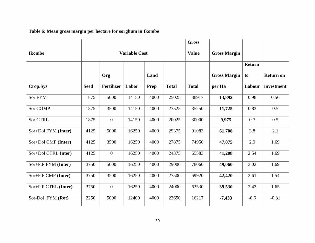
39

Table 6: Mean gross margin per hectare for sorghum in Ikombe

Ikombe Variable Cost

Gross

Value Gross Margin

Crop.Sys Seed

Org

Fertilizer Labor

Land

Prep Total Total

Gross Margin

per Ha

Return

to

Labour

Return on

investment

Sor FYM 1875 5000 14150 4000 25025 38917 13,892 0.98 0.56

Sor COMP 1875 3500 14150 4000 23525 35250 11,725 0.83 0.5

Sor CTRL 1875 0 14150 4000 20025 30000 9,975 0.7 0.5

Sor+Dol FYM (Inter) 4125 5000 16250 4000 29375 91083 61,708 3.8 2.1

Sor+Dol CMP (Inter) 4125 3500 16250 4000 27875 74950 47,075 2.9 1.69

Sor+Dol CTRL Inter) 4125 0 16250 4000 24375 65583 41,208 2.54 1.69

Sor+P.P FYM (Inter) 3750 5000 16250 4000 29000 78060 49,060 3.02 1.69

Sor+P.P CMP (Inter) 3750 3500 16250 4000 27500 69920 42,420 2.61 1.54

Sor+P.P CTRL (Inter) 3750 0 16250 4000 24000 63530 39,530 2.43 1.65

Sor-Dol FYM (Rot) 2250 5000 12400 4000 23650 16217 -7,433 -0.6 -0.31

40

Sor-Dol COMP (Rot) 2250 3500 12400 4000 22150 13217 -8,933 -0.72 -0.4

Sor-Dol CTRL (Rot) 2250 0 12400 4000 18650 9317 -9,333 -0.75 -0.5

Sor- P.P FYM (Rot) 1875 5000 12400 4000 23275 38243 14,968 1.21 0.64

Sor- P.P COMP(Rot) 1875 3500 12400 4000 21775 36683 14,908 1.2 0.68

Sor- P.P CTRL (Rot) 1875 0 12400 4000 18275 31683 13,408 1.08 0.73

Sor (Mono); Sorghum Monocrop, Sor+Dol (Inter); Sorghum Dolichos Intercrop, Sor-Dol (Rot); Sorghum Dolichos Rotation, Sor+P.P (Inter); Sorghum Pigeon

Pea Intercrop, Sor-P.P (Rot); Sorghum Pigeon Pea Rotation, FYM; Farm Yard Manure COMP; Compost Manure CTRL; Control

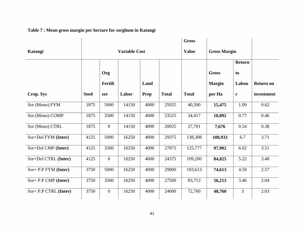
41

Table 7 : Mean gross margin per hectare for sorghum in Katangi

Katangi Variable Cost

Gross

Value Gross Margin

Crop. Sys Seed

Org

Fertili

zer Labor

Land

Prep Total Total

Gross

Margin

per Ha

Return

to

Labou

r

Return on

investment

Sor (Mono) FYM 1875 5000 14150 4000 25025 40,500 15,475 1.09 0.62

Sor (Mono) COMP 1875 3500 14150 4000 23525 34,417 10,892 0.77 0.46

Sor (Mono) CTRL 1875 0 14150 4000 20025 27,701 7,676 0.54 0.38

Sor+Dol FYM (Inter) 4125 5000 16250 4000 29375 138,308 108,933 6.7 3.71

Sor+Dol CMP (Inter) 4125 3500 16250 4000 27875 125,777 97,902 6.02 3.51

Sor+Dol CTRL (Inter) 4125 0 16250 4000 24375 109,200 84,825 5.22 3.48

Sor+ P.P FYM (Inter) 3750 5000 16250 4000 29000 103,613 74,613 4.59 2.57

Sor+ P.P CMP (Inter) 3750 3500 16250 4000 27500 83,713 56,213 3.46 2.04

Sor+ P.P CTRL (Inter) 3750 0 16250 4000 24000 72,760 48,760 3 2.03

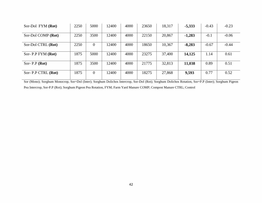
42

Sor-Dol FYM (Rot) 2250 5000 12400 4000 23650 18,317 -5,333 -0.43 -0.23

Sor-Dol COMP (Rot) 2250 3500 12400 4000 22150 20,867 -1,283 -0.1 -0.06

Sor-Dol CTRL (Rot) 2250 0 12400 4000 18650 10,367 -8,283 -0.67 -0.44

Sor- P.P FYM (Rot) 1875 5000 12400 4000 23275 37,400 14,125 1.14 0.61

Sor- P.P (Rot) 1875 3500 12400 4000 21775 32,813 11,038 0.89 0.51

Sor- P.P CTRL (Rot) 1875 0 12400 4000 18275 27,868 9,593 0.77 0.52

Sor (Mono); Sorghum Monocrop, Sor+Dol (Inter); Sorghum Dolichos Intercrop, Sor-Dol (Rot); Sorghum Dolichos Rotation, Sor+P.P (Inter); Sorghum Pigeon

Pea Intercrop, Sor-P.P (Rot); Sorghum Pigeon Pea Rotation, FYM; Farm Yard Manure COMP; Compost Manure CTRL; Control

43

The test of mean differences was done using GENSTAT; results are shown in table 8. Results are

shown for differences at five (p<o.o5) percent level of significance. Mean difference between

the farming systems, intercrop, and rotation was Ksh 25, 020.20 and was significant. The profit

difference between compost and farmyard manure was also significant and was Ksh 2,570.10.

Interaction of sites, farming systems and organic inputs was Ksh 37, 354.70 and significant.

There was no significant difference in gross margin observed between Ikombe and Katangi sites.

44

Table 8 : Mean gross margin results for sorghum based cropping system in Ikombe and Katangi

Ikombe Katangi

Farming system COMPOST CONTROL FYM Means COMPOST CONTROL FYM Means

Sorghum 11,725 9,975 13,892 11,864 10,892 7,767 15,475 11,378

Sorghum+Dolichos (Inter) 47,075 41,208 61,708 49,997 97,092 84,825 108,933 96,950

Sorghum+ Pigeon Pea (Inter) 42,420 39,530 49,060 43,670 56,213 48,760 74,613 59,862

Sorghum- Dolichos (Rot) -8,933 -9,333 -7,433 -8,567 -1,283 -8,283 -5,333 -3,367

Sorghum-Pigeon Pea (Rot) 14,908 13,408 14,968 14,428 11,038 9,593 14,125 11,586

Means 21,439 19,270 26,127 22,279 34,790 28,532 42,523 35,282

%C.v 17.1

L.s.d Site 37663.3Ns

L.s.d Farming System 25020.2*

L.s.d Input 2570.1*

L.s.d Site x Farming System x Input 37354.9*

Least Significant Difference (LSD) * 5% level of error Intercrop (Inter), Rotation (Rot)

45

Reject the hypothesis that there is no significant difference in profit in adoption of agroecological

intensification technique and conclude that AEI techniques result greater revenues.

4.2.2 Mean gross margin per hectare for cassava

Results for gross margins for cassava in Ikombe and Katangi under different crop systems and

organic inputs in sorghum based system are shown in Table 9 and 10. In Ikombe the highest

(Ksh 89,008) gross margin per hectare was using cassava dolichos intercrop with farm yard

manure while the least (Ksh 7,825) was in cassava pigeon pea rotation with compost organic

input. In Katangi, the highest gross margin per hectare (Ksh 434,135) was in cassava pigeon pea

intercrop with farm yard manure and the lowest (Ksh 10,895) was in cassava pigeon pea rotation

with on organic input (Control).

Cassava root is tolerant to poor soils and adverse weather conditions. Yield per unit of land is

high compared to other crops including sorghum hence greater gross margins from cassava. It is

also adapted to wide range of agroecological zones.

46

Table 9 : Mean gross margin per hectare for cassava in Ikombe

Ikombe Variable Cost

Gross

Value Gross Margin

Crop. System Seed

Org.

Fertilizer Labour

Land

Prep Total Total

Gross

Margin/

ha

Return

on Lb

Return on

investment

Cassava (Mono) FYM 95000 5000 29000 4000 133000 220095 87,095 3 0.65

Cassava (Mono) COMP 95000 3500 29000 4000 131500 177436 45,936 2 0.35

Cassava (Mono) CTRL 95000 0 29000 4000 128000 196209 68,209 2 0.53

Cass+Dol FYM (Inter) 97250 5000 33900 4000 140150 229158 89,008 3 0.64

Cass+Dol COMP (Inter) 97250 3500 33900 4000 138650 197170 58,520 2 0.42

Cass+Dol CTRL (Inter) 97250 0 33900 4000 135150 159741 24,591 1 0.18

Cass+ P.P FYM (Inter) 96875 5000 33900 4000 139775 211588 71,813 2 0.51

Cass+ P.P COMP (Inter) 96875 3500 33900 4000 138275 205525 67,250 2 0.49

Cass+ P.P CTRL (Inter) 96875 0 33900 4000 134775 186435 51,660 2 0.38

Cass-Dol FYM (Rot) 2250 5000 12900 4000 24150 78600 54,450 4 2.25

47

Cass-Dol COMP (Rot) 2250 3500 12900 4000 22650 87900 65,250 5 2.88

Cass-Dol CTRL (Rot) 2250 0 12900 4000 19150 63900 44,750 3 2.34

Cass- P.P FYM (Rot) 1875 5000 12900 4000 23775 36118 12,343 1 0.52

Cass- P.P COMP (Rot) 1875 3500 12900 4000 22275 30100 7,825 1 0.35

Cass- P.P CTRL (Rot) 1875 0 12900 4000 18775 27520 8,745 1 0.47

Mono; Monocrop, Cass+Dol (Inter); Cassava Dolichos Intercrop, Cass-Dol (Rot); Cassava Dolichos Rotation, Cass+P.P (Inter); Cassava Pigeon Pea Intercrop,

Cass-P.P (Rot); Cassava Pigeon Pea Rotation, FYM; Farm Yard Manure COMP; Compost Manure CTRL; Control

48

Table 10 : Mean gross margin per hectare for cassava in Katangi

Katangi Variable Cost

Gross

Value

Gross

Margin

Crop. System Seed

Org.

Fertil

izer Labour

Land

Prep Total Total

Gross

Margin/

ha

Return

on

Labor

Return on

investment

Cassava FYM 95000 5000 29000 4000 133000 325880 192,880 7 1.45

Cassava COMP 95000 3500 29000 4000 131500 266791 135,291 5 1.03

Cassava CTRL 95000 0 29000 4000 128000 248030 120,030 4 0.94

Cass+Dol FYM (Inter) 97250 5000 33900 4000 140150 264700 124,550 4 0.89

Cass+Dol COMP (Inter) 97250 3500 33900 4000 138650 198265 59,615 2 0.43

Cass+Dol CTRL (Inter) 97250 0 33900 4000 135150 148020 12,870 1 1.1

Cass+ P.P FYM (Inter) 96875 5000 33900 4000 139775 573910 434,135 13 3.11

Cass+ P.P COMP (Inter) 96875 3500 33900 4000 138275 483546 345,271 10 2.5

Cass+ P.P CTRL (Inter) 96875 0 33900 4000 134775 479756 344,981 10 2.56

Cass-Dol FYM (Rot) 2250 5000 12900 4000 24150 95850 71,700 6 2.97

49

Cass-Dol COMP (Rot) 2250 3500 12900 4000 22650 78750 56,100 4 2.48

Cass-Dol CTRL (Rot) 2250 0 12900 4000 19150 46350 27,200 2 1.42

Cass- P.P FYM (Rot) 1875 5000 12900 4000 23775 42570 18,795 1 0.79

Cass- P.P (Rot) 1875 3500 12900 4000 22275 36980 14,705 1 0.66

Cass- P.P CTRL (Rot) 1875 0 12900 4000 18775 29670 10,895 1 0.58

Mono; Monocrop, Cass+Dol (Inter); Cassava Dolichos Intercrop, Cass-Dol (Rot); Cassava Dolichos Rotation, Cass+P.P (Inter); Cassava Pigeon Pea Intercrop,

Cass-P.P (Rot); Cassava Pigeon Pea Rotation, FYM; Farm Yard Manure COMP; Compost Manure CTRL; Control

50

Test for mean differences in gross margin under cassava based system in Ikombe and Katangi

are shown in Table 11. The results show significant difference at five (p<o.o5) percent level of

error. The difference in gross margins between Ikombe and Katangi sites was Ksh 190, 043.10,

between farming systems Ksh 110,904 and between inputs, farmyard and compost was 41,

585.40. The difference in effect of interaction of site, farming system and organic inputs was

196,883.20. These differences were all significant at five percent.

51

Table 11: Mean gross margin results for cassava based cropping system in Ikombe and Katangi

Ikombe Katangi

Farming system COMPOST CONTROL FYM Means COMPOST CONTROL FYM Means

Cassava 45,936 68,209 87,095 67,080 135,291 120,030 192,880 140,400

Cassava + Dolichos (Inter) 58,520 24,591 89,008 57,373 59,615 12,870 124,550 65,678

Cassava + Pigeon Pea (Inter) 67,080 51,660 71,813 63518 345,271 344,981 434,135 374,795

Cassava – Dolichos (Rot) 65,250 44,750 54,450 54,817 56,100 27,200 71,700 51,666

Cassava – Pigeon Pea (Rot) 7,825 8,745 12,345 9,638 14,705 10,895 18,795 14,798,

Means 35,906 39,591 62,942 56,742 122,197 103,195 168,412 129,467

%C.v 32.2

L.s.d Site 190043.1*

L.s.d Farming System 110904*

L.s.d Input 41585.4*

L.s.d Site x Farm System x Input 196883.2*

Least Significant Difference (LSD) * 5% level of error Intercrop (Inter), Rotation (Rot)

52

Again reject the null hypothesis that there is no significant difference in profit between

agroecological techniques and conclude that there is difference in gross margin.

The results confirm findings of Place et al., (2003) and Pannell et al., (2014) that showed that

application of crop management vary across agroecological conditions. Different site, systems

and organic inputs combinations yield unique results. Interventions for soil management

practices need to be designed to address the unique inputs and systems farmers may use.

4.2.3 Mean gross margin based on farmers’ data

Table 12 shows results for average gross margin in sorghum at for farmers’ different levels of

AEI techniques. At zero (0) level, the farmer adopted none of the components of AEI while at

level six the farmer adopted all six components.

53

Table 12 : Farmers’ mean gross margin for sorghum under AEI techniques in Yatta

Level of AEI 0 1 2 3 4 5 6

Revenue

Yield kg ha-1 20.0 70.86 69.81 91.09 102.04 155.77 180.72

Total revenue (Ksh ha-1) 445 1559 1536 2004 2245 3427 3976

Variable Costs

Seeds

40.50 58.30 91.10 141.70 83.00 89.50 100.00

Fertilizers

0.00 0.00 0.00 103.20 57.90 0.00 0.00

Chemicals

0.00 0.00 0.00 0.00 0.00 0.00 0.00

Manure

0.00 200.00 260.70 485.80 688.30 299.60 330.00

Labour

323.90 603.20 300.00 313.00 446.60 384.00 550.00

Total Variable cost (Ksh ha-1) 364.40 861.50 651.80 1043.70 1275.70 773.10 980.00

Gross margin (Ksh ha-1) 80.63a 697.46b 884.15c 960.28c 969.29d 2653.93e 2996.00e

N=32 Significant of mean difference a,b,c,d,e =1%

54

Table 12.1: ANOVA Results for differences in gross margins of sorghum for farmers at

different levels of adoption

Sum of Squares df Mean Square F Sig.

Between Groups 2.789E7 6 4647768.472 1927.502 .000

Within Groups 320701.738 133 2411.291

Total 2.821E7 139

There was a significant (p<o.o1) difference in gross margins for sorghum between groups of

farmers at different levels of AEI adoption. However for farmers that applied between three or

four practices of AEI technique in sorghum no difference in gross margin was noted. Farmers

that applied at least five or six practices accrued significantly (p<0.01) higher Ksh 2653 ha-1 and

Ksh 2996ha-1 profits respectively. The high incomes attained by farmers applying several

components of AEI maybe due to the enhanced soil moisture and organic carbon content due to

the practices. However, compared to trial results, farmers earn lower gross margins from

sorghum. The gap may suggest lack of knowledge by farmers on the proper application of AEI

technique.

Table 13 shows farmers’ average gross margins for cassava at different levels of AEI technique.

In Cassava, profits were significantly (p<o.o1) different between farmers at different levels of

AEI technique. Farmer that practiced at least one technique attained Ksh 448 ha-1 compared to

Ksh 152 ha-1 for farmers that applied none.

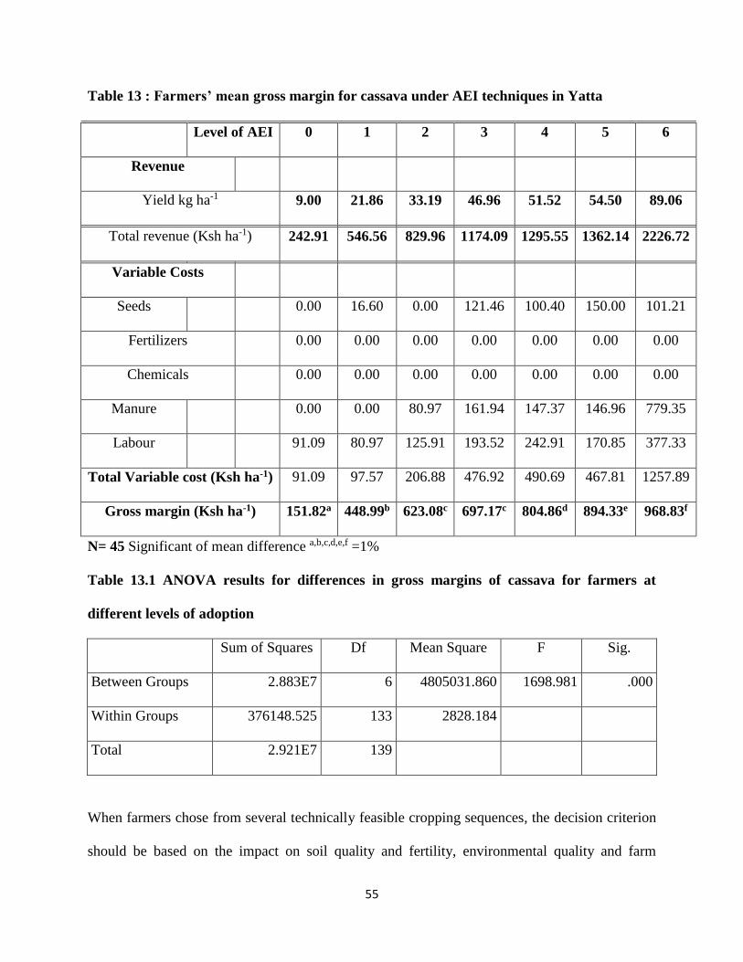
55

Table 13 : Farmers’ mean gross margin for cassava under AEI techniques in Yatta

Level of AEI 0 1 2 3 4 5 6

Revenue

Yield kg ha-1 9.00 21.86 33.19 46.96 51.52 54.50 89.06

Total revenue (Ksh ha-1) 242.91 546.56 829.96 1174.09 1295.55 1362.14 2226.72

Variable Costs

Seeds

0.00 16.60 0.00 121.46 100.40 150.00 101.21

Fertilizers

0.00 0.00 0.00 0.00 0.00 0.00 0.00

Chemicals

0.00 0.00 0.00 0.00 0.00 0.00 0.00

Manure

0.00 0.00 80.97 161.94 147.37 146.96 779.35

Labour

91.09 80.97 125.91 193.52 242.91 170.85 377.33

Total Variable cost (Ksh ha-1) 91.09 97.57 206.88 476.92 490.69 467.81 1257.89

Gross margin (Ksh ha-1) 151.82a 448.99b 623.08c 697.17c 804.86d 894.33e 968.83f

N= 45 Significant of mean difference a,b,c,d,e,f =1%

Table 13.1 ANOVA results for differences in gross margins of cassava for farmers at

different levels of adoption

Sum of Squares Df Mean Square F Sig.

Between Groups 2.883E7 6 4805031.860 1698.981 .000

Within Groups 376148.525 133 2828.184

Total 2.921E7 139

When farmers chose from several technically feasible cropping sequences, the decision criterion

should be based on the impact on soil quality and fertility, environmental quality and farm

56

profitability. Both researcher and farmers data show that agroecological technique is profitable.

The explanation for the gap in yield and profit suggest that farmers lack information on

application of technique necessary to increase their yields.

In ASAL areas inclusion of neglected traditional crops such as sorghum and cassava that are

drought resistance and tolerant to low soil fertility can enhance the competitiveness of the

system. In a study on sorghum based systems nutrient balances in Yatta Namoi et al., (2014),

found significantly lower Nitrogen (N) and Phosphorus (P) balances. This may explain the lower

incomes in sorghum systems compared to the cassava systems. Hence the choice of crop and

organic input combination in a system is important when deciding the enterprise the farmer

should operate.

4.3 Adoption of agroecological intensification technique in Yatta, Sub- County

The empirical results of the regression model are presented in Table 14. Test for

multicollinearity was done using the correlation matrix and the variance inflation factor (VIF). In

presence of high collinearity, the standard errors are often inflated and estimated coefficients can

be unreliable. Although the pair-wise correlations give guide to presence of multicollinearity,

high zero-order correlations are a sufficient but not a necessary condition for the existence of

multicollinearity because it can exist even though the zero-order or simple correlations are

comparatively low, say, less than 0.50, Gujarati (2007). Therefore several tests are employed to

test multicollinearity. According to Gujarati (2007), the rule of thumb is if the VIF of a variable

exceeds 10, which will happen if R2j exceeds 0.90, that variable is said be highly collinear. The

VIF of the variables was less than 10 and the pair-wise correlation less than 0.7.

The chi-squared value was significant at 1%, implying that all the variables jointly determine the

dependent variable. McFadden R2 of 10.88%, is sufficiently high. However, the Poisson Model

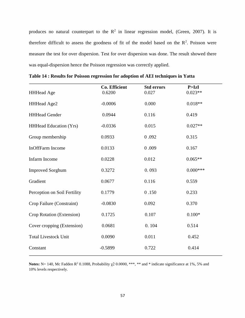
57

produces no natural counterpart to the R2 in linear regression model, (Green, 2007). It is

therefore difficult to assess the goodness of fit of the model based on the R2. Poisson were

measure the test for over dispersion. Test for over dispersion was done. The result showed there

was equal-dispersion hence the Poisson regression was correctly applied.

Table 14 : Results for Poisson regression for adoption of AEI techniques in Yatta

Co. Efficient Std errors P>ІzІ

HHHead Age 0.6200 0.027 0.023**

HHHead Age2 -0.0006 0.000 0.018**

HHHead Gender 0.0944 0.116 0.419

HHHead Education (Yrs) -0.0336 0.015 0.027**

Group membership 0.0933 0 .092 0.315

InOffFarm Income 0.0133 0 .009 0.167

Infarm Income 0.0228 0.012 0.065**

Improved Sorghum 0.3272 0. 093 0.000***

Gradient 0.0677 0.116 0.559

Perception on Soil Fertility 0.1779 0 .150 0.233

Crop Failure (Constraint) -0.0830 0.092 0.370

Crop Rotation (Extension) 0.1725 0.107 0.100*

Cover cropping (Extension) 0.0681 0. 104 0.514

Total Livestock Unit 0.0090 0.011 0.452

Constant -0.5899 0.722 0.414

Notes: N= 140, Mc Fadden R2 0.1088, Probability χ2 0.0000, ***, ** and * indicate significance at 1%, 5% and

10% levels respectively.

58

The following variables were found have significant influence on adoption; age and education

level of household head, farm income, and extension training on crop rotation, and cultivating

improved sorghum.

Age was found to positively influence adoption of agroecological intensification technique and

was statistically significant at 5 percent level. However, since the sample average age high, the

function age squared was included to help model more accurately the influence of age. This was

necessary because result show that older farmer was more likely to adopt the technique. To test

whether the effect of age is linear for all ages, age squared was included. The result showed that

at much higher age the level of adoption was negatively and significant at five percent level of

error. Hence we conclude that the influence of age is not infinite and much older farmers are less

likely to adopt. This may suggest that AEI should be targeted at farmer at the average age.

Number of years of formal education of the household head was found significant at 5 percent

but the influence on adoption negative. This is contrary to the priori expectation that education

would enhance adoption. Education enhances farmers’ management skills, and improves ability

to access and evaluate information (Wozniak, 1984). These should enhance adoption. However

technology attributes can affect adoption. According to Lancaster (1979) a consumer considerers

the bundle of attributes of a commodity rather than a commodity itself. Assuming that educated

farmers are consumers of technology, the Lancaster theory may help explain the observed effect

of education on adoption of AEI techniques. The AEI technique relies on indigenous knowledge

and is perceived to have increased demand for labour (Tripp, 2005). This attributes may not be

attractive to educated farmers who may prefer modern innovations and less labour intensive

techniques compared to traditional techniques.

59

Level of farm income was found positively affect adoption and significant at 10 percent. Studies

have shown that farmers seek alternative income to supplement farm income (Fernandez-

Cornejo, 2007). It allows for farm resources to be available for reinvestment into the farm. The

results here suggest that farm households not only depend on off farm income but also on farm

income. Farm income therefore provides farmers incentives to invest in the soil management

technology. The positive and significant influence on adoption can be used a proxy for resources

available to farmer to practice the AEI technique.

Extension training on crop rotation was found positive and significant at 10 percent while

cultivating improve sorghum variety positively and significantly affected adoption at 1 percent.

This is consistent with other studies that show extension accelerates adoption (Odendo, 2010,

Otieno et al. 2011). Farmers are more likely to adopt technology once they have full information

about a technique. Training enhances skill and supplements farmers’ traditional/indigenous

knowledge. Cultivation of improved sorghum varieties may enhance adoption as farmers would

like to exploit the full potential of the cultivars. This can motivate them to address the soil

fertility through uptake of better management practices.

In conclusion we reject the hypothesis that socio economic factors do no influence adoption. We

conclude socio economic factors: age, education, farm income resources and access to extension

affect the adoption and intensity of uptake of agro-ecological intensification technique.

60

5.0 SUMMARY, CONCLUSIONS AND RECOMMENDATIONS

5.1 Summary

The purpose of this study was to evaluate profitability and factors affecting adoption of

Agroecological Intensification Techniques in Yatta Sub-County, Kenya. Six agroecological

intensification techniques; crop rotation, cover cropping, crop residue incorporation, crop

diversity, compost manure and farm yard manure were considered in the study. Out of a sample

of 140 households, twenty nine percent adopted all six techniques considered in this study. The

average number of techniques adopted was four. Farm yard manure was the most adopted by

ninety five percent of households, then crop diversity at seventy seven percent, compost manure

seventy six percent, incorporation of crop residue seventy two percent, cover cropping fifty

seven percent and crop rotation was least adopted with only fifty four percent of households

taking it up.

To assess profitability gross margin analysis were calculated and then ANOVA was conducted to

assess difference in mean gross margins between different categories of farmers. Two sets of

data used; on-farm trial and farmer field data. In farm trials for Sorghum, the highest mean gross

margin, Ksh 108,933ha-1, was attained in Katangi in sorghum dolichos intercrop system with

addition of farmyard manure. In cassava based system the highest Ksh 434,135ha-1 in Katangi

with pigeon pea intercrop treated with farmyard manure. In survey mean gross margin was Ksh

2996ha-1 and Ksh 968ha-1 in Sorghum and Cassava for farmers adopting all six techniques

studied. Test of difference show a significant (p<o.o1) difference in gross margin between

farmers at different levels of adoption.

A Poisson regression model was estimated to measure the influence of socioeconomic factors on

adoption. The factors found to influence adoption were age, education, farm income, extension

61

training and cultivation of improved sorghum. Therefore as contrary to the hypothesis

socioeconomic factors affect the uptake of the AEI technique.

5.2 Conclusion

Both on-farm trials and farmers’ gross margin analysis showed higher revenue were the

agroecological intensification technique was applied. Farm yard manure results were higher than

cultivation without addition of organic inputs. In sorghum intercropping with dolichos gave

higher revenue than in rotation or with pigeon pea. In cassava system result show that cassava

dolichos intercrop with farmyard manure in Ikombe and cassava pigeon pea intercrop with farm

yard manure in Katangi gave the highest revenue. Farmers’ gross margins for both sorghum and

cassava were highest when the farmer applied all the techniques including farmyard manure,

compost, cover cropping, crop rotation, incorporating crop residue and intercropping. This lead

to rejection of the hypothesis, there is no significant difference in gross margins between

application and non-application of agroecological intensification technique. The conclusion is

agroecological intensification technique is a profitable approach to soil management.

To increase farmers’ yields and incomes, it is important that information appropriate technique

and crops to use is availed through researcher’s collaboration during technique development. The

gap in revenue between farmers at different levels of adoption and between farmers and

controlled research experiments reveal that there is potential for higher incomes. Greater

collaboration between farmers and researchers could help improve productivity and increase

incomes. Combination of enterprises should be also considered when deciding on crop rotation

and intercrop systems.

Targeting farmers of average age and access to information provide the most excellent platform

for further uptake of agroecological technique. Farm income and cultivation of improved

62

sorghum was found to enhance adoption, hence creating markets for these commodity may

further motivate farmers to adopt soil conservation techniques. Lack of formal education is found

not limiting to the adoption of AEI technique. While education is important these result suggest

that these technique is available to all farmers despite their education level.

5.3 Recommendations

5.3.1 Policy recommendations

Following these findings the study recommends: Investments in sustainable soil management

activities need to be targeted; different AEI technique for different agroecological zones.

Inclusion of legumes in crop rotation and intercropping systems helps to attain higher returns. In

sorghum systems it should be encouraged to intercrop with dolichos in both Ikombe and Katangi.

In cassava systems in Ikombe it should be intercropped with dolichos while in Katangi it should

be intercropped with pigeon peas. In all systems addition of farm yard manure would improve

the yields hence incomes. Extension training on agroecological intensification technique should

target individuals within the average age of fifty four years, and those with less than less

education. Trainings on each technique that addresses soil fertility challenge e.g. training on crop

residue/rotation to address soil fertility should be done separately rather than collectively.

Improved crop varieties should be encouraged because it enhances farmers have incentive to

address soil fertility. For instance improved seed varieties could be promoted together with an

appropriate legume intercropping variety.

5.3.2 Recommendations for further research

Further research areas in the agroecological technique may model different management

scenarios of AEI techniques and assess profitability under the different combination. Research

may also assess the returns over time for the different combinations. The study recommends cost

63

benefits analysis where discounting can be done. The finding would provide insights about

possible techniques combinations under different resource abundance and farmers’ objectives.

Similar studies may also be carried out in other arid and semi-arid areas and acess whether such

studies yield same results allowing for genitalization. It would also provide farmers with

information on how they can be combine approaches to reduce cost and increase economic

efficiency.

64

REFERENCES

Adesina. A, and Baidu-Forson. J, ‘Farmers' perceptions and adoption of new agricultural

technology: evidence from analysis in Burkina Faso and Guinea, West Africa,’ Vol

13 Agricultural Economics, 1995, pp 1-9

Adesina. A, and Chianu. A, ‘Farmers’ use and adaptation of alley farming in Nigeria,’ In Barrett

Adolwa. I, P.Okoth, R.Mulwa, A.Esilaba, F. Mairura and E. Nambiro., ‘Analysis of

Communication and Dissemination Channels Influencing the Adoption of Integrated

Soil fertility Management in Western Kenya,’ Journal of Agricultural Education and

Extension, Vol 18:1, 2012, pp 71-86

AGRA, ‘Climate Change and Smallholder Agriculture in Sub-Saharan Africa, ‘ AGRA, Africa

Agriculture Status Report, 2014.

Ajayi. C and Matakala. P., ‘Environmental Conservation and Food Security in Developing

Countries: Bridging the Disconnect,’ Conference Paper, International Association of

Agricultural Economists Conference, Gold Coast Australia, Aug, 2006.

Alene. A and Manyong. V, ‘The effects of education on agricultural productivity under

traditional and improved technology in northern Nigeria: an endogenous switching

regression analysis,’ Empirical Economics, Vol 32, 2007, 141-159

Amit, R., “Africa Fertilizer summit Outcomes and Follow-up,”

http://www.tzdpg.or.tz/uploads/media/ifdc.pdf, 2006.

Ayuya, O, S. Waluse and E. Gido, in ‘Multinomial Logit of Small Scale Farmers’ Choice of

Organic Soil Management Practices in Bungoma County, Kenya’ in Journal of Social

Sciences Vol 4(4), 2012, pp 314-322.

65

Bonabana - Wabbi, J, ‘Assessing Factors Affecting Adoption of Agricultural Technologies: The

case of Integrated Pest Management (IPM) in Kumi District Eastern Uganda’, Virginia

Polytechnic Institute and State University, 2002.

Bortkiewicz, L, Das Gesetz der Kleinen Zahlen, [The Law of Small Numbers] Teubner: Leipzig,

1898

Burke. W., ‘Fitting and Interpreting Cragg’s Tobit Model Alternaive using Stata,’ The Stata

Journal, 9 No.4, 584-592, 2009.

Cameron. A and P. Trivedi, ‘Essentials of Count Data Regression,’ June 1998*

Chege. J, ‘An Assessment of the Impact of Export Horticulture Farming on Food Security of

Smallholder Farmers in Mbooni, Kirinyaga and Buuri, Kenya,’ U.ON, 2014.

CIMMYT, Economics Program, ‘The Adoption of Agricultural Technology: A Guide for Survey

Design’. Mexico, D.F.: CIMMYT, 1993.

Côte. F, K. Tomekpe, C. Staver, S. Depigny1, T. Lescot, R. Markham, ‘Agro-Ecological

Intensification in Banana and Plantain (Musa spp.): an Approach to Develop More

Sustainable Cropping Systems for Both Smallholder Farmers and Large-Scale

Commercial Producers’ Acta Hort. 879, ISHS, 2010.

De Groote, H., S. Kimenju, G. Owuor., and J. Wanyama, Market Liberalization and Agricultural

Intensification in Kenya (1992 -2002), 2006

De Jager, A., D. Onduru, M. S. van Wijk, J. Vlaming, and G. N.Gachini, “Assessing

sustainability of low-external-input farm management systems with the nutrient

monitoring approach: a case study in Kenya,” Agricultural Systems 69(2001):99-118,

2001.

66

Duflo. E, M. Kremer and J. Robinson, “Understanding Technology Adoption: Fertilizer in

Western Kenya. Preliminary Results from field Experiments,’ May 2004

Esilaba. O, J. Byalebeka, A. Nakiganda, S. Mubiru, J. Delver, H. Ssali and M. Mbalule,

‘Integrated Nutrient Management Strategies in Easter Uganda,’ 17th WCSS

Symposium Aug, 2002.

et al., 2002, pp. 51–64.

FAO, ‘Climate change in Africa: The threat to Agriculture?’ FAO, 2009.

ftp://ftp.fao.org/docrep/fao/012/ak915e/ak915e00.pdf

FAO, ‘Opportunities and Threats of Irrigation Development in Kenya’s Drylands,’ F.A.O Vol VI:

Turkana County, 2013

FAO, ‘The Ethics of Sustainable Agricultural Intensification,’ F.A.O Ethics Series, 2004

FAO, ‘World Agriculture, Towards 2015/2030, An FAO Perspective, F.A.O, Ed. J.Bruinsma,

Eartscan Publications Ltd London, 2003

Feder. G, Just. R, and Zilberman. D, ‘Adoption of agricultural innovations in developing

countries: A survey. Economic Development and Cultural Change, 33(2), 1985, 255-

298

Firbank. L, S. Petit, S. Smart, A. Blain and R. Fuller, ‘Assessing the Impacts of Agricultural

Intensification on Biodiversity: A British Perspective, The Royal Society, Vol 363 Feb

2007, pp 777-787

Fischer. G, E. Hizsnyik, S. Prieler and D. Wilberg, ‘Scarcity and Abundance of land resources:

Competing uses and the Shrinking land resources base,’ F.A.O SOLAW Background

Thematic Report, 2015.

67

Foster, A.D. and Rosenzweig. M.R., ’A Economic Growth and the Rise of Forests,’ Quarterly

Journal of Economics, 118(2): 2003, pp 601-637

Franzluebbers. K, R. Hossner and A. Juo, ‘Integrated Nutrient Management for Sustained Crop

production in Sub-Saharan Africa,’ Soil Management CRSP, TropSoils/TAMU

Technical Bulletin 98-03, Department of Soil and Crop Sciences, Texas A&M

University, July 1998

Gebremedhin.B and G.Schwab., ‘The Economic Importance of Crop Rotation Syatems:

Evidence From the Literature,’ Department of Agricultural Economics, Michigan

State University, Staff Paper No 98-13, Aug 1998

Geiger. F, J. Bengtsson, F. Berendse, W. Weisser, M. Emmerson, M. Morales, P. Ceryngier, J.

Liira, T. Tscharntke, C. Winqvist, S. Eggers, R. Bommarco, T. Part, V. Bretagnolle,

M. Plantegenest, L. Clement, C. Dennis, C. Palmer, J.Onate, I. Guerrero, V. Hawro,

T. Aavik, C. Thies, A. Flohre, S. Hanke, C Fischer, P. Goedhart, and P.Inchausti,

‘Persistent negative effects of pesticides on biodiversity and biological control

potential on European farmland’, Basic and Applied Ecology, Vol 11, 2010, pp 97-

105.

Gliessmann, S.R, ‘Agroecology: Ecological Processes in Sustainable Agriculture,’ Ann Arbor

Press, 1998

GoK, ‘Kenya Population Situation Analysis,’ Government of Kenya, National Council for

Population and Development, July 2013.

Green. W. H, ‘Econometric Analysis, 6th Ed New York University, June 2007

Gruhn. P, F. Goletti and M. Yudelman, ‘Integrated Nutrient Management, Soil Fertility and

Sustainable Agriculture: Current Issues and Future Challenges,’ Food, Agriculture

68

and the Environment Discussion Paper 32, International Food Policy and Research

Institute (IFPRI), Sep 2000

Gujarati. D, Basic Econometrics, 4th edition McGraw Hill, 2007

Harms. B, A. Stortelder and W. Vos, ‘ Effects of intensification on Nature and Landscape in the

Netherlands,’ SCOPE, Land Transformation in Agriculture, Eds, M. Wolman and F.

Fournier, John Wiley & Sons Ltd, 1987

Holloway, G. J., Nicholson, C., Delgado, C., Ehui, S., Staal, S, ‘Agroindustrialization through

Institutional Innovation: Transaction Costs, Cooperatives and Milk Market

Development in the East African Highlands. Agricultural Economics 23, 2000, pp

279 – 288

Howard, M., Matikinca, P., Mitchell, D., Brown, F., Lewis, F., Mahlangu, I., Msimang, A.,

Nixon, P. and Radebe, T., ‘Small-scale timber Production in South Africa: what role

in reducing poverty?’ Fractal Forest Africa, Fakisandla Consulting, Institute of

Natural Resources, Rural Forest Management cc, South Africa, and IIED, London,

2005.

Hycenth. T, J. Schuler, S. Uthes and P.Zander.,’ Adoption Decision Theories and Conceptual

Models of Innovation systems,’ CA2Africa Inception Workshop, Mar, 2010

ILEA “Is agricultural intensification ecologically sustainable?,” ILEIA Newsletter • 14 nº 2-3 •

September 1998,

Institute of Development Studies (IDS), ‘Horizon’ University of Sussex, Aug, 2009

Irungu. P, ‘An Economic analysis of factors affecting the adoption of napier grass in Smallholder

dairying in Kiambu District, Kenya, U.O.N 1999

69

Jaetzold, R., H. and Schmidt, B. ‘Ministry of Agriculture Farm Management Handbook of

Kenya’ VOL. II-2nd edition Part C Subpart C1. Nairobi, Kenya: Ministry of

Agriculture, 2006.

Karanja- Lumumba. T, ‘Adoption and Profitability of Smallholder Dairt Goat Production in

Kenya: The Case of Meru South and Meru Central Districts, U.O.N, 2010.

KARI, ‘Report on Status of Maize Lethal Necrosis Disease and General Performance,’ July 2012

Kariyasa. K and Y. Dewi, ‘Factors Affecting Adoptuion of Integrated Crop Management Farmer

Filed School (ICM-FFS) in Swampy Areas,’ International Journal of Food and

Agricultural Economics,’ Vol 1. No. 2. 2013, pp 29-38.

Kelly, V, E. Crawford, C. Donovan and T. Jayne, ‘Input profitability Analysis’, What works for

African Smallholders: Input use and market development’ Department of Agricultural

Economics, Michigan State university, June, 2003.

Kelsey. J. B, “Constraints on the adoption of agricultural technologies in developing countries,”

Literature review, Agricultural Technology Adoption Initiative, J-PAL (MIT) and

CEGA (UC Berkeley), 2013

Kibaara, B., and Nyoro, J., “Expanding the Agricultural Finance Frontier: A Kenyan Case,”

Institute of Agricultural Policy and Development, 2007.

Kibunja, C.N, F.B. Mwaura, D.N. Mugendi, ‘Long-term land management effects on soil

properties 293 and microbial populations in a maize-bean rotation at Kabete, Kenya,’

.Afr J Agric Res 5:108-113, 2010

Kiprotich. M, E. Mamati and E. Bikketi., ‘Effect of limate hange on Cowpea production in

Mwania Watershed: A Case of Machakos County.’ International Journal of

Education and Research, Vol 3 No. 2 Feb 2015.

70

Kiptot. E, Franzel. S, Hebinck. P and Richards. P, ‘Sharing seed and knowledge: farmer to

farmer dissemination of agroforestry technologies in Western Kenya,’ Agroforest Sys,

2006, (68) 167-179

KNBS, ‘Statistical Abstract,’ Kenya National Bureau of Statistics, 2010

KNBS, ‘Statistical Abstract,’ Kenya National Bureau of Statistics, 2013

Kristen, J., A. Dorward, C. Poulton, W. Omamo, and N. Vick, “Institutional Economics

Perspective on African Agricultural Development: Institutional and the Agricultural

Development Challenges in Africa,” 2008.

Kydd, J., A. Dorward, C. Poulton, “Overcoming Market Constraints on Pro-Poor Agricultural

Growth in Sub-Saharan Africa,” Development Policy Review Vol 24 (3): 243-277,

2006.

Lambrecht. I, B. Vanlauwe and M.Maertens, ‘Agricultural extension in eastern DR Congo: Does

Gender Matter?’ Paper prepared for presentation at the EAAE 2014 Congress “Agri-

Food and Rural Innovations for Healthier Societies”, Aug 2014

Lancaster, K.J.,’Variety, Equity and Efficiency,’ Columbia University Press, New York, 1979.

Macharia, P, Kenya. Gateway to Land and Water Information: Kenya National Report, 2010.

FAO, (Food and Agriculture Organization) http://www.fao.org/ag/agL/

swlwpnr/reports/y_sf/z_ke/ke.htm

Maina.F and S. Kimani, ‘Enterprise prioritization and implication for soil fertility management-

The case of Kiambu District’ Abstracts Innovation as key to the green revolution in

Africa: Exploring the scientific facts , eds, Andre Bationo, Jeremiah M. Okeya, Boaz

S. Waswa, Paul Mapfumo, Fredah Maina and Job Kihara 2008, pp 169.

71

Marenya, P. and C. Barrett, “The Effect of Soil Quality on Fertilizer Use Rates among

Smallholder Farmers in Western Kenya,” American Journal of Agricultural

Economics, Vol 91(4):991-1006, 2009.

Mbuvi. P, ‘Makueni District Profile: Soil Fertility Management,’ Drylands Research Working

Paper 6., 2000.

Miguel. A and Clara. N, ‘Agroecology and the Search for a Truly Sustainable Agriculture,’

UNEP, 2008

Mugwe .J, Mugendi.D, Kungu.J and Onguso-Oeba.V, “Household and farm characteristics

influencing uptake of soil fertility management technologies by farmers in Meru South

District, Kenya, 2008

Munyao. C, F. Muisu, J. Mbogo and N. Kiprutto, ‘Comparison of Jatropha Cureas Profitability

to Selected Crops in Yatta District, Kenya,’ Journal of Economic and Sustainable

Development Vol 4 No. 8, 2013

Mwang’ombe. A, I.Wagara, J. Kimenju and R. Buruchara, ‘Occurence and Severity of Angular

Leaf Spot of Common Bean in Kenya as Influenced by Geographical Location,

Altitude and Agroecological Zones,’ Plant Pathology Journal 6 (3), 2007: 235-241

Namoi. N, R. Onwonga, C. Onyango, G. Karuku and V. Kathumu, ‘Assessment of Soil Nutrient

Balances in Organic Based Cassava (Manihot esculenta Crantz) and Sorghum

(Sorghum bicolor (L.) Moench) Cropping Systems of Yatta Subcounty, Kenya,’

American Journal of Experimental Agriculture, 4(12): 2014, pp 1557-1578

Ndambiri. H, C. Ritho and S. Mbogoh, “An Evaluation of Farmers’ Perception and Adaptation

To The Effects of Climate Change in Kenya,” International Journal of Food And

Agricultural Economics, Vol 1. No1, 2013, pp 75-96

72

Neupane, R. P., Sharma, K. R. and Thapa, G. P., ‘Adoption of agroforestry in the hills of Nepal:

a logistic regression analyses’ Agricultural Systems 2002 pg 72:177–196.

Nkonya. E, Gerber. N, Von Braun. J. and Pinto. A., ‘The Economics of Land Degradation; The

Cost of Action versus Inaction,’ International Food Policy Research Institute, Issue,

brief 68, September, 2011

Nkonya. E, J. Koo, E. Kato and Z. Guo, ‘Trends and Petterns of land use change and

international aid in Sub-Saharan Africa,’ United Nations University WIDER Working

Paper, 2013/ 110

Odendo. M, Obare. G, and Salasya. B, ‘Factors responsible for the differences in uptake of

integrated soil fertility management practices amongst Smallholder farmers in Western

Kenya’ African Journal of Agricultural Research Vol. 4 (11), Nov 2009, pp. 1303-

1311.

Odendo.M, Obare.G, and Salasya. B., ‘Determinants of the Speed Of Adoption Of Soil Fertility

enhancing Technologies In Western Kenya.’ The 3rd A.A.E & 48th A.E.A.S.A

Conference, The Westin Grand Cape Town Arabella Quays, South Africa, 19-23

September 2010

Oluoch- Kosura. W, Marenya.P and Nzuma.J, ‘Soil Fertility Management in Maize based

production systems in Kenya: Current and Future strategies’ Seventh Eastern and

Southern Africa regional Maize conference, Feb 2001 pp 350-355.

Oluyede. C, F. Akinnifesi, G. Sileshi and S. Chakerdza, ‘Adoption of renewable soil fertility

replenishment technologies in Southern African region: Lessons Learnt and the way

forward,’ Natural Resources Forum 31, 2007, pp 306-317.

73

Omamo. S.W, J. C. Williams., G. A. Obare. and N. N. Ndiwa., “Soil fertility on small farms in

Africa: evidence from Nakuru District in Kenya,” Elsevier, Food Policy 27(2002)

159-170

Omotayo, O. E. and Chukwuka, K. S., “Soil fertility restoration techniques in Sub Saharan

Africa using organic resources,” “African Journal of Agricultural Research,” Vol 4

(3):144-150, 2009.

Onwu, A.C, Ayuba ,S.A. and Ali, A., “The Effect of Organic Manure on the Growth and Yield

of Castor Plant (Ricinus Cumunis),” Journal of Sustainable Development in

Agriculture and Environment, Vol 3(2):64-70, 2008.

Otieno. Z, J. Okello, A. Mwang’ombe and D. Clavel, ‘The role varietal traits in the adoption of

Dryland Crop varieties: The Case of Pigeon Pea in Kenya,’ AfJARE Vol 6 No 2

September, 2011

Pannell, D., Llewellyn, R.S, Corbeels, M., ‘The farm-level economics of conservation

agriculture for resource-poor farmers,’ Agriculture, Ecosystems and Environment.

2014: 187(1), 2-56

Place F., Franzel, S., DeWolf, J., Rommelse, R., Kwesiga, F., Niang, A., Jama, B. Agroforestry

for soil fertility replenishment: evidence on adoption processes in Kenya and Zambia.

In: Barrett, C.B., Place, F., Aboud, A.A. (Eds.), Natural Resources Management in

African Agriculture: Understanding and Improving Current Practices CAB

International, Wallingford, UK, 2003, pp. 155–168.

Pretty. J, C. Toulmin and S. Williams, ‘Sustainable Intensification in African Agriculture,’

International Journal of Agricultural Sustainability, Vol 9, 2011, pp 5-24.

Rogers. E, ‘ Diffusion of Innovations,’ Fourth Edition, The Free Press, 1995

74

Sunding. D, & Zilberman. D, ‘The agricultural innovation process: Research and technology

adoption in a changing agricultural sector,’. In B. Gardner & G. Rausser (Eds.),

Hand- Book of agricultural economics, Volume 1. Amsterdam: North Holland

Publishing Company, 2001

The Royal Society, ‘Reaping the Benefits: Science and Sustainable Intensification of Global

Agriculture, The Royal Society, Oct 2009.

Tripp, R., Self-Sufficient Agriculture: Labour and Knowledge in Small-scale Farming,

Earthscan, London, 2005.

Tscharntke. T, A. Klein, A. Kruess, I. Steffan- Dewenter and C. Thies, ‘Landscape Perspective

of Agricultural Intensification and Biodiversity- Ecosystem Service Management,’

Ecology Letters Vol 8, 2005, pp 857-874

USDA, Soil Survey Manual. USDA Agricultural Handbook 18. Superintendent of Documents.

Washington, DC, 1978.

Virlanuta, F., F. Buhociu and L. Mihalcea, ‘Profitability Analysis for Agricultural Investment

Projects’ Risk in contemporary econ`omy’ University of Galati, 2011

Warren. P, ‘Livelihood Diversification and Enterprise Development: An Initial Exploration of

Concepts and Issues,’ F.A.O LSP Working paper 4, 2002

Wodaja. T., ‘ADouble Hurdle Model of Computer and Internet Use in America,’ Department of

Economics, Western Michigan University, 2009

World reference base for soil resources (WRB) – A framework for international classification,

correlation and communication, 2006 (E)

Wozniak. G, ‘The Adoption of Interrelated Innovations: A Human Capital Approach’ The MIT

Press, The Review of Economics and Statistics, Vol. 66, No. 1, Feb., 1984, pp. 70-79.

75

APPENDICES Appendix 1: Research Survey Questionnaire

Household Questionnaire

Dear respondent, this questioner is designed to seek your response on factors affecting adoption

of agro ecological technique. The response will be used for academic purposes only. Your

participation will be highly appreciated.

INTERVIEW BACKGROUND

Date Of the interview Interviewer

Time Started Time ended

Date checked

Date entered

County

District

Division

Location

Sub location

Village

Respondent’s name:

Contact (Mobile number)

Age

Farming experience (Yrs)

76

HOUSEHOLD IDENTIFICATION, COMPOSITION AND LABOR CONTRIBUTION (Objective 2 & 3)

Household members= people who live together and share meals including hired labour, children living away but supported by the household but

excluding visitors.

Memb

er

code

Name of household member

(start household head)

Sex

Cod

e A

Age Marital

Status

Codes B

Education

(Years)

Codes C

Number of

months lived in

the household

Occupation (Time spent)

Codes D

Household

Farm labour

contribution

Codes E Main Secondary

1

2

3

4

5

6

7

8

77

Code A Code B Code C Code E Code E

1. Female

2. Male

1. Married living

with spouse

2. Married but

spouse away

3. Divorced

4. Widow/wido

wer

5. Single

6. Other

(specify)….

1. None/illitera

te

2. Adult

education or

1 year of

education

*Give other

education in

years

1. Farming (Crop livestock)

2. Salaried employment

3. Self employed off-farm

4. Casual labourer on-farm

5. Casual labourer off-farm

6. Scholl/college child

7. Non-school child

8. Herding

9. Household chores

10. Others (specify)…

1. 100%

2. 75%

3. 50%

4. 25%

5. 10%

6. Not a worker

78

LAND HOLDING AND USE IN THE LAST CROPPING SEASONS (Objective 2 & 3)

1) What is the total size of your land? ____________________________Acres

2) What is the type of land tenure? Code A ________________________

Codes A

1. Own with title deed

2. Own without title

deed

3. Family land

4. Communal

5. Rented/ Hired

6. Others (Specify) ……

79

3) How did you use your land during in the last two seasons?

Land

Catego

ry

March –May 2010

Long rain

Oct- Dec 2010 short

rains

March- May 2011 long

rains

Oct- Dec 2011

short rains

March- May

2012 long rains

Oct- Dec 2012 short rains

Cultivated

(annual +

permanent

crops)

Unculti

vated

Cultivated

(annual +

permanent

crops)

Uncultiv

ated

Cultivated

(annual +

permanent

crops)

Uncultiva

ted

Cultivat

ed

(annual

+

permane

nt crops)

Uncultiv

ated

Cultivate

d (annual

+

permanen

t crops)

Un

cul

tiv

ate

d

Cultivated

(annual +

permanent

crops)

Uncultiv

ated

Own

land

Rented

in land

Rented

out land

Borrow

ed in

land

Borrow

ed out

land

80

SOCIO CAPITAL AND NETWORKING (Objective 2 & 3)

4) Do any of the household members belong to a group? Yes (1) No (0); Please describe the group.

Does any member of the household currently belong to any group? 0=N0 1=Yes

Member Code

(from module

2)

Type of group the

household member

is registered:

Codes A

Three most important functions of the group: Codes B Year joined

(YYYY)

Role in the group

Codes C

1st 2nd 3rd

Codes A Codes B Codes C

1. Input supply/farmer

coops/union

2. Crops/seed producer and

marketing group/coops

3. Farmers’ Association

4. Women’s Association

5. Youth Association

6. Church/mosque

association/congregation

7. Saving and credit group

8. Funeral association

9. Government

10. Water user’s association

11. Others (specify)….

1. Produce marketing

2. Input access/marketing

3. Seed production

4. Farmer research group

5. Savings and credit

6. Funeral group

7. Tree planting and nurseries

8. Soil & water conservation

9. Church group/congregation

10. Input credit

11. Others (specify)…

1. Official

2. Ex-official

3. Ordinary member

81

ACCESS TO EXTENSION SERVICES (Objective 2 & 3)

5) How do you access agricultural training or information?

Rank Source

Name/Description

Code A Frequency of

information

access Code B

Reliability of

source Code C

Relevance of

information

Code D

1

2

3

4

5

Code A Code B Code C Code D

1. Government

extension officers

1. Daily 1. Fully reliable 1. Fully relevant

2. Radio 2. Weekly 2. Very reliable 2. Very relevant

3. Newspaper,

Bulletins

3. Bi-weekly 3. Fairly reliable 3. Fairly

relevant

4. Agro vets/ Seed

dealers

4. Monthly 4. Somewhat

reliable

4. Somewhat

relevant

5. Farmers’

organization

5. Quarterly 5. Unreliable 5. Irrelevant

6. Neighbours 6. Half-

annually

7. NGO e.g. church 7. Annually

8. Research

institutions e.g.

KARI,

Universities

8. Others

(Specify)…..

9. Demonstration

farms

10. Mobile phone,

Internet

11. Indigenous

knowledge

90. Others

(Specify)……..

82

6) Did you receive training on the following issues in the last three years?

Issue Received

training

or

informati

on on

[…]

since

2010

0=N0

1=Yes

Main source of information for […] Number of interactions during 2011/2012

Codes A

1st Number of

contacts

2nd Number of

contacts

3rd Number of

contacts

New crop

varieties

Crop rotation

Field pest and

diseases

Leaving crop

residue

Soil and water

management

Cover crops

Crop diversity

Manure

production /use

Compost use

Adaptation to

climate change

Livestock

production

Tree planting/

Agro forestry

83

Code A

1. Government extension officers

2. Radio

3. Newspaper, Bulletins

4. Agro vets/ Seed dealers

5. Farmers’ organization

6. Neighbours

7. NGO e.g. church

8. Research institutions e.g. KARI,

Universities

9. Demonstration farms

10. Mobile phone, Internet

11. Indigenous knowledge

90. Others (Specify)……..

ACCESS TO FINANCIAL CAPITAL, INFORMATION AND INSTITUTIONS (Objective 2 & 3)

7) Did you apply for credit in the last one year? Yes (1) No (0)………………….

8) If yes, please fill the table below, if no, skip to Question 9.

Reason for loan Needed

credit for

[..]0= No

1=Yes

Did you

get the

credit

0=N0

1=Yes

Source of

credit

Code A

Did you

get the

amount

you

applied

for? 0=N0

1=Yes

How

much did

you get?

(Ksh)

Monthly

interest

rate (%)

Repayment

period

(months)

1. Buying seeds

2. Buying

fertilizer

3. Buying other

inputs

4. Labour

wages

5. Buy food

6. Others

specify ….

Code A

1. Money lender

2. Farmer group/coop

3. Merry go round

4. Microfinance

5. Bank

6. SACCO

7. Relative

8. AFC

9. Others (specify)……

84

9) Who decides what inputs to buy?

Household member code or

Do not buy ( Code 99)

1. Fertilizer

2. Seed

3. Pesticides

4. Farm implements

HOUSEHOLD ASSETS (Objective 2 & 3)

10) Household item owned.

Assets Total Number owned How much would you sell it in its

current state? (Ksh) (if >1 take

average)

1 Fork jembe

2 Hoe

3 Spade

4 Axe

5 Knapsack sprayer

6 Ox plough

7 Panga

8 Slasher

9 Donkey/ Ox cart

10 Push Cart (mkokoteni)

11 Bicycle

12 Motorbike

13 Truck/car

85

14 Wheelbarrow

15 Posho mill

16 Improved charcoal/ wood

store

17 Kerosene stove

18 Gas cooker

19 Electric stove

20 Radio, cassette player

21 Mobile phone

22 TV

23 Land

86

AWARENESS OF AGRO ECOLOGICAL INTENSIFICATION TECHNIQUE (Objective 2)

11) Are you aware of agro ecological intensification of land use techniques? (Enumerator prompts by defining

AEI technique)

Agro

ecological

technique

Are you

aware of

[…] Yes

(1) No (0)

Do you

apply […]

technique

Have you

ever attended

an on-farm

demonstration

on […]Yes

(1) No (0)

If yes continue …

Main

source of

information

Codes A

If yes

how

many

training

sessions

did you

attend?

Did you

try any

of the

practices

taught

on […?]

How

many

years

have you

practiced

[…?]

11a 11b 11c 11d 11e 11f 11g

1 Crop rotation

2 Crop

diversity

3 Cover

cropping

4 Compost

manure

5 Crop residue

use

6 Manure

7 Improved

cassava

variety

8 Sorghum

variety

Code A

1. Government extension

officers

2. Radio

3. Newspaper, Bulletins

4. Agro vets/ Seed dealers

5. Farmers’ organization

6. Neighbours

7. NGO e.g. church

8. Research institutions e.g.

KARI, Universities

9. Demonstration farms

10. Mobile phone,

Internet

11. Indigenous

knowledge

90. Others

(Specify)……..

17) Which of the following was a constraint in your farm?

87

Issue Is […} a constraint in your farm? 0=N0

1=Yes

1. Pest

2. Diseases

3. Soil fertility

4.Soil erosion

5. Crop failure

6. Lack of water

7. Others (specify)…

20) FARMING SYSTEMS (Objective 2)

A. Inter cropping: What crops did you grow in the last six seasons in intercrop?

Season

Code

A

Crop Grown

Crop

Code

(Crop

annex)

Acreage

(Acres)

Plant

spacing

Codes B

Average Yield Per

unit area

Reason For Growing

Crop

Codes C

1

2

3

4

5. Others

(Specify)……

1

2

3

4

5. Others

(Specify)……

1

2

3

4

88

5. Others

(Specify)……

1

2

3

4

5. Others

(Specify)……

1

2

3

4

5. Others

(Specify)……

Codes A Codes B Codes C

1. Long rains

2010

2. Short rains

2010

3. Long rains

2011

4. Short rains

2011

5. Long rains

2012

6. Short rains

2012

1.Broadcasting

2.Mixed spacing

3.Row planting

4.Strip spacing

5.Hill planting

1. Consumption

2. Income

3. Food diversification

3. Soil fertility management

4. Integrated pest management (IPM)

4. Fodder

5. Others (specify)…

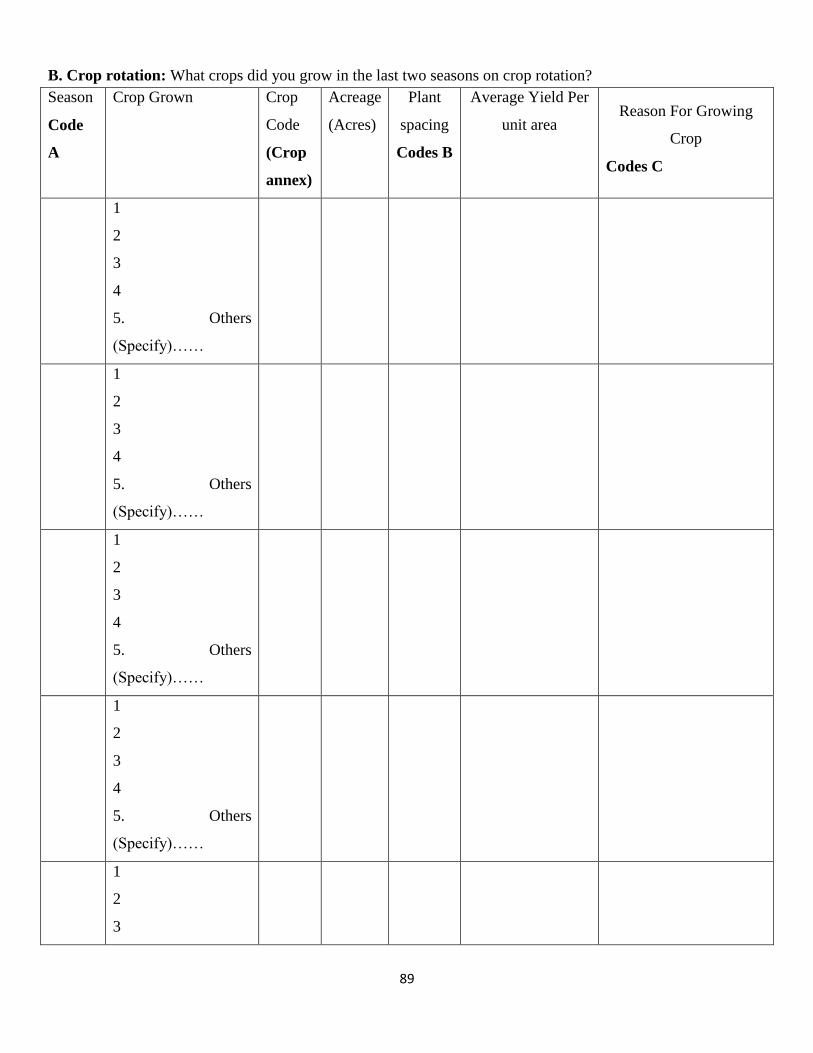
89

B. Crop rotation: What crops did you grow in the last two seasons on crop rotation?

Season

Code

A

Crop Grown

Crop

Code

(Crop

annex)

Acreage

(Acres)

Plant

spacing

Codes B

Average Yield Per

unit area

Reason For Growing

Crop

Codes C

1

2

3

4

5. Others

(Specify)……

1

2

3

4

5. Others

(Specify)……

1

2

3

4

5. Others

(Specify)……

1

2

3

4

5. Others

(Specify)……

1

2

3

90

4

5. Others

(Specify)……

Codes A Codes B Codes C

1. Long rains

2010

2. Short rains

2010

3. Long rains

2011

4. Short rains

2011

5. Long rains

2012

6. Short rains

2012

1.Broadcasting

2.Mixed spacing

3.Row planting

4.Strip spacing

5.Hill planting

1. Consumption

2. Income

3. Food diversification

3. Soil fertility management

4. Integrated pest management (IPM)

4. Fodder

5. Others (specify)…

C. Mono cropping: What crops did you grow in the last two seasons in Monocrop?

Season

Code

A

Crop Grown

Crop

Code

(Crop

annex)

Acreage

(Acres)

Plant

spacing

Codes B

Average Yield Per

unit area

Reason For Growing

Crop

Codes C

1

2

3

4

5. Others

(Specify)……

1

2

3

4

5. Others

(Specify)……

91

1

2

3

4

5. Others

(Specify)……

1

2

3

4

5. Others

(Specify)……

1

2

3

4

5. Others

(Specify)……

Codes A Codes B Codes C

1. Long rains 2010

2. Short rains 2010

3. Long rains 2011

4. Short rains 2011

5. Long rains 2012

6. Short rains 2012

1.Broadcasting

2.Mixed spacing

3.Row planting

4.Strip spacing

5.Hill planting

1. Consumption

2. Income

3. Food diversification

3. Soil fertility management

4. Integrated pest management (IPM)

4. Fodder

5. Others (specify)…

PERCEPTION ON SOIL FERTILITY (Objective 2 & 3)

18) Please rank the soil fertility of your farm. Codes A

Codes A

1. Good

2. Medium

3. Poor

19) Please evaluate the gradient of your farm. Codes B

Codes B

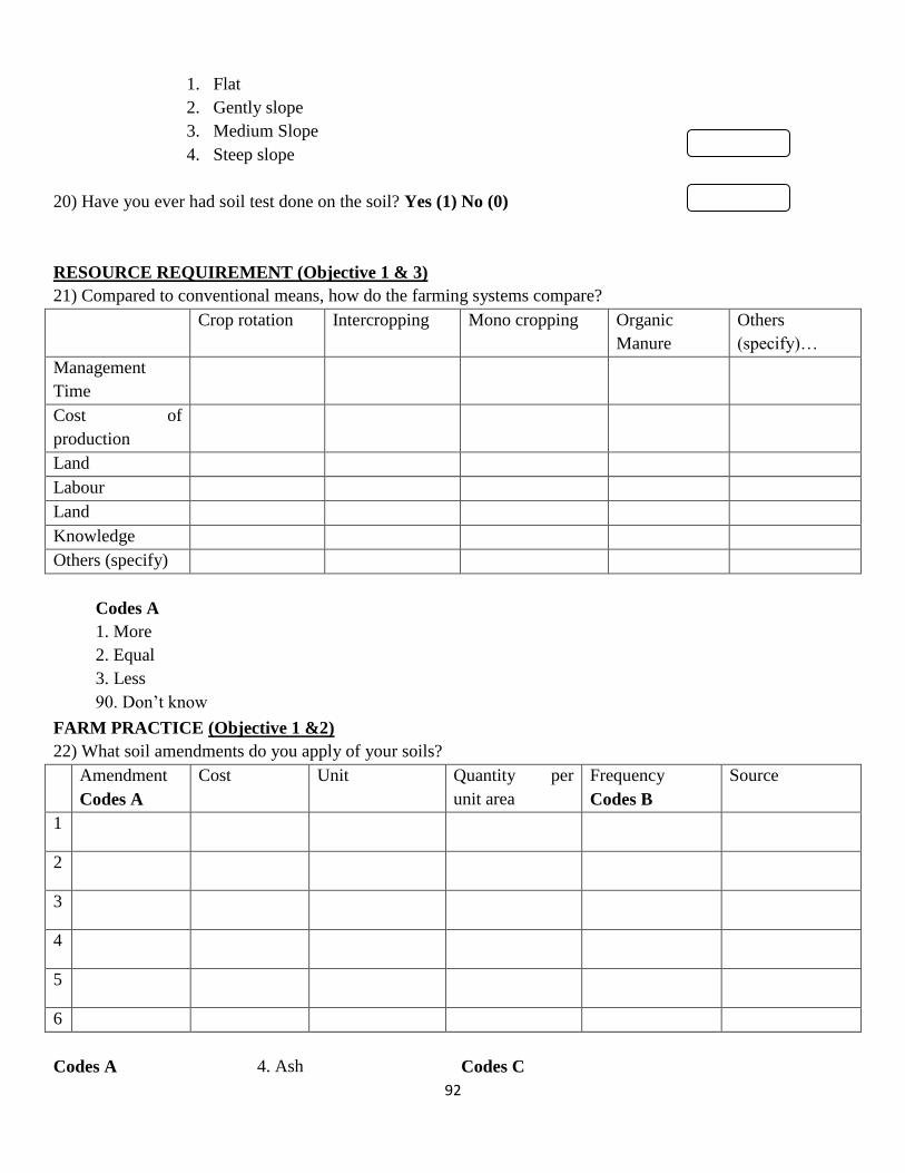
92

1. Flat

2. Gently slope

3. Medium Slope

4. Steep slope

20) Have you ever had soil test done on the soil? Yes (1) No (0)

RESOURCE REQUIREMENT (Objective 1 & 3)

21) Compared to conventional means, how do the farming systems compare?

Crop rotation Intercropping Mono cropping Organic

Manure

Others

(specify)…

Management

Time

Cost of

production

Land

Labour

Land

Knowledge

Others (specify)

Codes A

1. More

2. Equal

3. Less

90. Don’t know

FARM PRACTICE (Objective 1 &2)

22) What soil amendments do you apply of your soils?

Amendment

Codes A

Cost Unit Quantity per

unit area

Frequency

Codes B

Source

1

2

3

4

5

6

Codes A 4. Ash Codes C

93

1. Fertilizer

2. Manure

3. Compost

5. Mulching

6. None

7. Others (specify)…

1. Per season

2. Annually

94

CROP PRODUCTION INPUT USE (Objective 1)

Cost of crop production in the last two seasons?

Se

aso

n

Pl

ot

co

de

Pl

ot

si

ze

Cr

op

Na

me

Cr

op

co

de

Inter

crop

o=N

o 1=

Yes

Seed Fertilizer

Labour use in man/days Manure

Pestici

de Harvest

Land

prepar

ation

Plan

ting

Wee

ding

Harve

sting

To

tal

la

bo

ur

co

st

O

w

n Bought

Sou

rce

Co

de

B

Q

ty

in

K

gs

Price

/unit

To

tal

see

d

Co

st

Q

ty

Pri

ce

pe

r

un

it

Total

Ferti

lizer

cost

K

g

Q

ty

To

tal

Co

st

Q

ty

lit

re

To

tal

Co

st

Q

ty Price

/unit

95

Codes A Codes B

1. Long rains

2. Short rains

1. Own seed

2. family/ neighbour

3. Farmer to farmer seed exchange

4. On farm trials/ extension demonstration

plots

5. farmer group

6. Agro- dealers/agro-vets

7. Provided free by NGOs

8. Government subsidy program

9. Government/ research

institutions

10. Others (specify)…

96

UTILIZATION OF CROP RESIDUES FROM MAIN CROPPING SEASON (%) (Objective 1 & 3)

23) Note that percentages need to add up to 100% for every row

Crop

Code

Annex 1

Burnt in

the field

(%)

Used as

firewood

(%)

Left on

land for

soil

fertility

(%)

Feed for

livestock

(%)

Used for

construction

(%)

Sold

(%)

Used to

make

compost

(%)

Others

uses (%)

LIVESTOCK AND LIVESTOCK PRODUCTS (Objective 2 & 3)

24) Please describe your household’s livestock assets

Livestock Number

owned

Average selling

price

Ksh/unit

Who makes

decisions on

livestock?

Eg.sell

Main livestock

product

Codes A

1st 2nd 3rd

1 Dairy cattle

2 Indigenous

cattle

3 Bulls

4 Calves

5 Small animals

97

e.g. Goats,

sheep

6 Poultry

7 Donkey

8 Camel

9 Rabbit

10 Others

(specify) …

MARKETING (Objective 1 & 2)

Marketing: one row per crop per season

Season

Code A

Crops Code

(Crops

annex)

Crops

Variety

Code B

Market

type Code

C

Quantity

sold (kg)

Who sold

(HH

member

code)

Price

(Ksh/Kg)

Total

marketing

cost

Codes A Codes B Codes C

1. Long rains

2. Short rains

1. Improved variety

2. Local Variety

1. Farm gate

2. Village Market

3. Main/district market

Codes A Codes B

1. Milk

2.Manure

3. Blood

4. Eggs

5. Hides

6. Others (specify)…

1. Household

2. Spouse

3. Others (specify)….

Member codes module 2

98

HOUSEHOLD INCOME FOR THE LAST 12 MONTHS (Objective 3)

25) Source of income for the last 12 months

Type of Income Did you or

any

household

member

earn from

this last

year? 0=N0

1=Yes

Number of

days

worked per

year

Average income per

unit

Total

income

earned

Cash

(Ksh)

Payment in

kind – cash

equivalent

1 Agricultural labour

2 Casual labour

3 Salary

4 Pension

5 Remittance

income/gifts

6 Rent

7 Small business

8 Sale of wood and

charcoal

9 Sale of forest

products e.g. wild

fruits

10 Sale in shop, petty

trade

11 Transport

12

Sal

e of

farm

pro

duct

s

Crops

13 Animal manure

14 Crop residue

15 Animal fodder

16 Sale of cows

17 Sale of poultry

18 Sale of animal

products

19 Others (specify)…

99

HHLDH

Age

HHLDH

Age2

HHLDH

Gender

HHLDE

duYrs

Per.Soil

Fert

InOffFar

mInc Gradient

InFarm

Inc

CropRot

(Ext)

CoverCro

p(Ext)

Improv

edSor

T.Livest

ockU

Group

Mem

Crop

Failure

HHLDHeadAge 1

HHLDHeadAge2 0.9909 1

HHLDHeadGender -0.2223 -0.211 1

HHLDEduYrs -0.6357 -0.65 0.2629 1

PerceptionSoilFertility -0.007 -0.013 0.0286 0.08 1

InOffFarmIncome -0.0264 -0.04 0.1098 -0.041 -0.089 1

Gradient 0.1583 0.133 -0.167 -0.1 0.1634 0.0022 1

InFarmIncome 0.0006 0.005 0.0652 0.14 0.1336 -0.0572 -0.0947 1

CropRotation Ext 0.0687 0.063 0.1477 -0.022 0.2029 0.0701 0.1696 0.169 1

CoverCrops Ext 0.0983 0.076 0.0239 -0.057 0.2472 -0.0169 0.2546 0.086 0.4945 1

ImprovedSor -0.0112 -0.027 0.1215 0.057 0.224 0.0814 0.1997 0.09 0.4103 0.3816 1

TotalLivestockUnit 0.0577 0.048 0.133 0.011 0.1537 -0.0486 0.0867 0.132 0.1933 0.2159 0.1541 1

GroupMembership 0.0637 0.078 -0.0189 -0.011 0.0617 0.0075 -0.0161 0.156 0.034 -0.0344 0.0653 0.1172 1

CropFailure Constraint 0.0605 0.067 0.0037 -0.02 -0.2 -0.0166 -0.1066 0.166 -0.086 -0.1809 -0.04 -0.118 0.0715 1

Appendix 2: Variable Correlation Matrix

100

Appendix 3: Variable Variance Inflation Factor (VIF)

Variable VIF 1/VIF

HHHEdu Yrs 1.81 0.55

HHLDHeadAge 1.77 0.57

HHLDHeadSex 1.19 0.84

CoverCrops 1.53 0.65

CropRot 1.51 0.66

ImprovedSorghum 1.34 0.74

Perception 1.18 0.84

Gradient 1.18 0.84

InFarmIncome 1.17 0.85

InOffFarmIn 1.05 0.95

CropFailure 1.14 0.87

TotalLivestockU 1.13 0.88

GroupMember 1.06 0.94

Mean VIF 1.31