An Analysis of Bitcoin Exchange Rates

Jacob Smith∗

University of Houston

March 31, 2015

Abstract

Bitcoins are digital gold. They are a purely electronic commodity traded for specu-lative purposes as well as in exchange for goods and services. Just like physical gold,the relative price of bitcoins denominated in different currencies implies a nominal ex-change rate. This is a departure from previous literature which treats bitcoin pricesthemselves as nominal exchange rates. I argue that treating prices as exchange ratesis inappropriate as one would not consider the price of physical gold to be an exchangerate. Therefore, this paper characterizes the behavior of nominal exchange rates im-plied by relative bitcoin prices. I show that the implied nominal exchange rate is highlycointegrated with the nominal exchange rate determined in conventional foreign cur-rency exchange markets. I also show that the direction of causality flows from theconventional markets to the bitcoin market and not vice-versa which can explain muchof the volatility in bitcoin prices.

Keywords: Bitcoin, Cointegration, Cryptocurrency, Exchange Rates

JEL Classification: E42, E47, C3

∗Special thanks for the helpful comments from David Papell, Dietrich Vollrath, German Cubas, and Chris-tian Murray as well as feedback from attendees of the UH Graduate Research Seminar and Hashers United In-ternational Bitcoin Conference. Please address correspondence to: Jacob Smith, Department of Economics,University of Houston, McElhinney 248, Houston, TX 77204-5019. Email: Jacob.BL.Smith@gmail.com.Copyright: Jacob B. Smith c©2014

1

1 Introduction

Bitcoins are digital gold, both in design and behavior. This paper will highlight the simi-

larities between the traditional commodity and its new digital counterpart. In doing so it is

evident that the bitcoin market is more mature than previously thought.

The contribution of this paper is to characterize the behavior of bitcoin-implied exchange

rates, i.e. the relative price of bitcoin denominated in different currencies. Whereas previous

authors have concerned themselves with top-level bitcoin prices, my analysis goes further

in studying relative bitcoin prices. I argue that the study of these relative prices is a more

appropriate endeavor when attempting to compare the behavior of bitcoin prices to conven-

tional currencies. In the same way that one would not call the price of physical gold an

exchange rate, neither do I call the price of bitcoins an exchange rate.

Three nominal exchange rates are considered for this analysis: The dollar-euro rate, the

dollar-pound rate, and the dollar-Australian dollar rate. These three rates were chosen based

on their economic importance and the availability of the data. The data are daily and span

the period from September 1st, 2011 to January 31st, 2014. While bitcoin prices themselves

are highly volatile and only weakly correlated with conventional nominal exchange rates, the

exchange rates implied by relative bitcoin prices are less volatile and are highly cointegrated

with conventional nominal exchange rates.

I employ Vector Error Correction modeling to describe the relationship between implied

and market exchange rates. For each exchange rate I estimate one cointegrating vector and

find that shocks to the conventional foreign exchange market have significant and permanent

effects on implied exchange rates in the bitcoin market. However, shocks to bitcoin-implied

exchange rates do not have any noticeable effects on conventional market rates. This one-

way causality implies that bitcoin prices must do all of the adjusting in order for implied and

market rates to return to parity. In this way, conventional exchange rate volatility drives

much of the bitcoin price volatility.

Previous comparisons of bitcoin prices to conventional exchange rates have shown little

2

similarity. This has led some to conclude that “bitcoin is not a real currency” Yermack

(2013). However, in thinking of bitcoin as digital gold the similarities become apparent. I

extend my analysis to include gold-implied exchange rates (i.e. relative gold prices) and

find that gold and bitcoin behave almost identically. Gold-implied exchange rates are highly

cointegrated with market exchange rates and shocks to the conventional market have large

persistent effects on the gold market but not vice versa. The similarities between gold and

bitcoin speak to the idea that bitcoin is not a currency in the sense that dollars and pounds

are currencies, but are much more akin to physical commodities liked gold, coffee, and oil.

The rest of the paper proceeds as follows: Section 2 provides a primer on the technology

of bitcoins and brief review of the literature. Section 3 presents the data and describes some

basic characteristics of bitcoin prices and exchange rates. Section 4 fits an in-sample model

and tests the predictability of bitcoin nominal exchange rates. Section 5 concludes.

2 What is a Bitcoin?

The recent surge in the popularity of bitcoins has garnered the attention of business profes-

sionals and academics unlike any other cryptocurrency. However, most of the discussion on

bitcoins has been confined to the computer science literature or blogosphere with almost no

academic research devoted to the economics of bitcoin.

The first question one might ask is “What is a Bitcoin?” Ron and Shamir (2012) provide

a concise definition:

“Bitcoins are digital coins which are not issued by any government, bank, ororganization and rely on cryptographic protocols and a distributed network ofusers to mint, store, and transfer.”

In other words, bitcoins are a purely digital, highly-liquid asset that are traded for spec-

ulative purposes and used as a currency. They are not backed by any tangible asset nor are

they sanctioned as legal tender. Thus, bitcoins are non-commodity and non-fiat.

The technology behind bitcoins was first introduced by the pseudonymous Satoshi Nakamoto

3

in 2009. Fundamentally, the bitcoin network is centered around a massive but decentralized

public ledger called the “Block Chain.” This ledger records every bitcoin transaction that’s

ever occurred since the network’s genesis. Each bitcoin is given a unique serial number. The

Block Chain publicly displays which bitcoins are associated with which accounts. When a

transaction occurs the Block Chain is appended to show that a particular bitcoin has moved

from one account to another. In this way, the bitcoin market is not unlike the stone wheels

of Yap.

The novelty of bitcoin is in the way in which transactions are processed. Suppose Jake

wishes to to send a bitcoin to Josie. Jake announces his intent to the entire network.

The proposed transaction spreads through the network until it finds a “Miner.” A Miner

is someone who verifies transactions. The Miner first verifies that Jake has the right to

send that particular bitcoin by checking Jake’s “Private Key” which is analogous to an

ATM PIN. This lets the Miner know that Jake is the rightful owner of the account. Once

Jake’s private key is verified the Miner sets about verifying the authenticity of the particular

bitcoin that Jake is trying to send. The Miner does this through a difficult “proof-of-work”

algorithm which scrolls through the Block Chain to check the bitcoin’s history. Proof-of-

work algorithms are hard to complete but easy to check. Any tampering with the bitcoin’s

code or any attempt to spend the same bitcoin twice will generate large deviations from

the algorithm’s expected result. For example, I know 2+2=4 but if I get sneaky and try to

add 2.0000001+2 the proof-work-algorithm will report an answer something like 1,729. If

the algorithm generates the correct result (or “hash”) then the transaction is deemed to be

valid. The Miner then bundles this transaction along with other verified transactions into a

“Block.” This new Block is broadcast to the network and appended to the Block Chain. At

this point the bitcoin that was in Jake’s account is now publicly recognized to be in Josie’s

account and the transaction is complete. The entire process takes approximately ten minutes

to complete.

Verifying these transactions is quite costly, requiring specialized equipment, technical

4

expertise, and a significant amount of electricity. To compensate Miners for their efforts

they are awarded newly minted bitcoins every time they complete a Block. It is important

to note that the bitcoin supply is not governed by a central bank or any type of monetary

policy rule but by the efforts of Miners. This is by design and intended to make the supply

of bitcoin similar (at least in theory) to the supply of gold.

As time goes on, the reward for verifying transactions is automatically reduced until the

maximum number of 21 million bitcoins have been mined. From then on Miners will no longer

be rewarded by the system for processing transactions. At its current pace, the network is

expected to mine its last bitcoin in the year 2140. This hard limit on the total supply of

bitcoins is feared to put deflationary pressure on prices and to thus encourage hoarding.

Indeed, Ron and Shamir (2012) find that 78% of all bitcoins are held in accounts which

receive coins but never spend them. Questions about the long-run incentives in the bitcoin

market lead Kroll, Davey, and Felten (2013) to conclude that some form of governance will

be required for long-run sustainability of the market.

Others have also leveled criticisms against the economic viability of bitcoin. Meiklejohn

et al. (2013) show that interactions in the bitcoin market aren’t that anonymous as the

Block Chain provides a public record of all transactions. This is an issue for bitcoin as

the anonymity of illicit transactions was and is one of the major draws for its utility as a

currency (Christin 2012). Pirrong (2013) attacks the efficiency of the market arguing that

too few actors and small market cap leave the market vulnerable to manipulation. Even

more concerning, Eyal and Sirer (2014) describe a strategy in which bitcoin Miners may

unilaterally cheat the system to receive more than their fair share of mining proceeds.

Yermack (2013) questions the maturity of the market by asking “Is Bitcoin a Real Cur-

rency?” The author shows that there is almost no correlation between the price of bitcoins

and conventional exchange rates. Moreover, the volatility of bitcoin prices is an order of

magnitude higher than the volatility observed in conventional nominal exchange rates. This

leads Yermack to conclude that “bitcoin behaves more like a speculative investment than a

5

currency.”

This paper looks deeper into the behavior of the bitcoin market and endeavors to explain

the extraordinarily high price volatility. Understanding the technology and construction of

bitcoins is crucial to understanding the behavior of agents in the bitcoin market. Like other

commodities (such as gold), bitcoins are bought and sold primarily for investment purposes

and assume a secondary role as a currency. And like these other commodities, the relative

price of bitcoins denominated in different currencies implies an exchange rate. That is, the

dollar price of bitcoins ($/B) divided by the Euro price of bitcoins (AC/B) implies a dollar-euro

exchange rate ($/AC). Focusing on this bitcoin-implied exchange rate gives insight into the

behavior of the bitcoin market. Contrasting the behavior of bitcoin-implied exchange rates

with similar gold-implied exchange rates allows a more direct comparison between traditional

commodity money and the burgeoning market for cryptocurrency. I find that bitcoins are

subject to the same motivations and dynamics as physical gold which leads me to conclude

that the bitcoin market, though small, is relatively mature.

3 Data

Daily data on bitcoin prices were downloaded from bitcoincharts.com. The prices are those

which prevailed on the Mt. Gox1 exchange at 12:00 a.m. GMT (UTC). There are any

number of bitcoin exchanges with freely floating prices, however, Mt. Gox was by far the

largest and most active (Meiklejohn et al. 2013). Data on bitcoin prices denominated in

US Dollars, British Pounds, Euros, and Australian Dollars were collected for the period

September 1st, 2011 to January 31st, 20142. Implied exchange rates were then calculated

by dividing the Dollar price of bitcoins ($/B) by the foreign price of bitcoins (£/B, AC/B,

1Not only was Mt. Gox the largest and most active bitcoin exchange, it was also one of the most activebitcoin market places in general (Meiklejohn et al. 2013).

2Data are available after January 31st, 2014, however, in early February 2014 news broke that Mt. Gox’ssecurity protocols had been compromised allowing hackers to seize bitcoins stored in customers’ accounts.Thus, there was a subsequent run on Mt. Gox bitcoins which caused the price to plummet and forced Mt.Gox into bankruptcy.

6

A$/B). Conventional market exchange rates as well as gold prices were obtained from the

St. Louis Fed’s FRED database. The nominal exchange rates are the “noon buying rates in

New York City for cable transfers payable in foreign currencies.” While gold prices are 3:00

p.m. (London Time) fixing prices which prevailed in the London Bullion Market. Figures

1-5 illustrate the data and Table 1 provides some descriptive statistics.

The descriptive statistics in Table 1 reiterate the findings of Yermack (2013): bitcoin

prices are indeed extraordinarily volatile when compared with conventional market exchange

rates. A fact illustrated in Figure 1. However, if one considers the bitcoin implied exchange

rates one notices that the mean and standard deviation are almost identical to the market

exchange rates. This fact is born out in Figures 3-5. While it is true that bitcoin implied

rates remain slightly more volatile than conventional market rates, it is clear the the implied

and market rates follow each other very closely. This is despite the fact that bitcoin prices

themselves are almost totally uncorrelated with market exchange rates.

One sees a similar pattern with physical gold. Gold prices themselves are highly volatile

and seemingly uncorrelated with market exchange rates, however, gold-implied exchange

rates track closely with market rates.

The relationship between the implied and market exchange rate is motivated by arbi-

trage. When the bitcoin (or gold) implied exchange rate finds itself out of parity with the

conventional market rate there exists an opportunity for arbitrage. As agents take advantage

of these arbitrage opportunities the exchange rates are driven back together. For example,

suppose the implied dollar-euro rate was greater in the bitcoin market than in the conven-

tional market. This means the euro is relatively stronger in the bitcoin market than in the

conventional market. Thus, a trader could exchange dollars for euros in the conventional

market (where euros are relatively cheap) and take those euros to buy bitcoins in the bitcoin

market (where euros are relatively valuable). The purchase of bitcoins with euros drives up

the euro price of bitcoin thereby driving down the implied exchange rate.

Such arbitrage is common whenever commodities are traded in different currencies (Sjaas-

7

tad and Scacciavillani 1996). These arbitrage trades often result in the series being coin-

tegrated. Two non-stationary series are said to be cointegrated if a linear combination of

the series is stationary. If one considers the spread between implied and market rates (i.e.

$/ACmarket − $/ACimplied) in Figure 6 it seems clear that the linear combination of the se-

ries is stationary about 0. This is mirrored in Figures 7 and 8 for the dollar-pound and

dollar-Australian dollar rates respectively.

One interesting comparison that can be made between the gold and bitcoin implied rates

is the relative size of the so-called arbitrage bands. The bands are much larger far the bitcoin

implied rates than for the gold implied rates. The width of the arbitrage band is dictated by

transaction costs, i.e. arbitrage trades are only made once the profits exceed the transactions

costs. Thus, higher transaction costs allow for higher disparity. Because the arbitrage bands

are much larger for bitcoins than for gold it must be that transactions costs are higher in the

bitcoin market than in the gold market. The exact reasoning for this is outside the scope of

this paper but further research into the size and dynamics of the exchange rate spread could

prove an interesting topic for further discussion.

4 Empirical Analysis

Engle and Granger (1987) show that if two series are cointegrated then a simple regression

of ∆yt on ∆xt is misspecified. A system of I(1) unit root processes is said to be cointegrated

if there exists some linear combination of the series which is stationary, or I(0). If we let yt

be a vector of time series then the system is cointegrated if there exists some non-zero vector

β such that β′yt is stationary. The system is said to be in “equilibrium” when β′yt = 0 and

out of equilibrium when β′yt 6= 0. We can denote this “equilibrium error” as zt = β′yt.

8

Consider the bivariate system,

yt + αxt = εt, εt = εt−1 + ξt (1)

yt + βxt = νt, νt = ρνt−1 + ζt, |ρ| < 1 (2)

where ξt and ζt are white noise. Note that the reduced form of yt and xt will be functions

of both ε and ν. Because εt is I(1) it must be the case that yt and xt are also I(1). Now

consider (2) which is a linear combination of yt and xt. Because νt is stationary it must be

the case that yt + βxt is also stationary. Therefore, yt and xt are cointegrated with a vector

β′ = (1, β).

Engle and Granger (1987) show that we can rewrite the system as,

∆yt = αδzt−1 + η1t (3)

∆xt = −δzt−1 + η2t (4)

where δ = (1 − ρ)/(β − α) and the η’s are linear combinations of εt and νt. Recall that

zt = yt + βxt. Thus, equations (3) and (4) illustrate the vector error correction (VEC)

representation of the system which describes how the series respond to disequilibrium.

If, however, yt is a VAR(p) the VEC representation can be expanded and written as,

∆yt = αβ′yt−1 +

p−1∑i=1

Γi∆yt−i + εt

For this analysis, ∆yt is a 2x1 vector[

∆yt∆xt

]where the ∆yt is the first difference in the

natural log of the implied exchange rate and ∆xt is the first difference in the natural log of

the market exchange rate. The vectors α and β are also 2x1 and contain the adjustment

parameters and cointegrating vector respectively. A simple VAR of ∆yt and ∆xt would omit

αβ′yt−1 and therefore be misspecified if indeed the series are cointegrated.

The matrix Γp is a 2x2 matrix of lag parameters

9

Γp =

γyy,p γyx,p

γxy,p γxx,p

Applying the VEC method to implied and market exchange rates follows Sjaastad and

Scacciavillani (1996). In their paper, Sjaastad and Scacciavillani estimate a cointegrating

relationship between gold-implied exchange rates and the market rate then attempt to use

this vector to forecast the nominal market rate. The authors show that the adoption of

floating exchange rate regimes has contributed significantly to the volatility of gold prices. I

will show that this is also a major factor in the extreme volatility in bitcoin prices. Sjaastad

and Scacciavillani (1996) also find that that the direction of causality flows from the nominal

exchange rate market to the gold market, but not vice versa. We will see that the bitcoin

market exhibits the same behavior. At the end of this section, I replicate portions of Sjaastad

and Scacciavillani (1996) using my data and find similar results.

The contribution of this paper is to apply Sjaastad and Scacciavillani’s methodology

to the bitcoin market. Doing so will shed light on the dynamics of the market as well as

illustrate the similarities between purely digital bitcoins and other physical commodities.

Determining the order of the VAR means considering five lag-selection methodologies.

The five methodologies all involve minimizing some criterion, either the Likelihood-Ratio, the

Final Prediction Error (FPE), the Akaike Information Criterion (AIC), the Hannan-Quinn

Information Criterion (HQIC), or the Schwartz Bayesian Information Criterion (SBIC). The

lag length which minimizes the majority of these five criteria is taken to be the most appro-

priate. For the dollar-euro and the dollar-Australian dollar rates a lag length of 2 is selected.

For the dollar-pound rates I use a lag-length of 5.

From there I apply Johansen’s (1988, 1991, 1995) methodology to formally tests for the

existence of cointegration. The results of the Johansen tests show that for all three currencies

I strongly reject the null of no cointegrating vector but fail to reject the null of at most 1

cointegrating vector. The results of these tests can be found in Table 2.

10

The Johansen tests confirm the presence of cointegration for all three currencies making

VEC modeling the most appropriate technique. Table 3 reports the parameter estimates of

(5) when considering bitcoin implied rates and conventional market rates.

In examining to the results from Panel 3a we see that the estimates of α1 are negative

and highly significant for each of the exchange rates. Recall that α1 is the way in which the

first series responds to disequilibrium, i.e. the implied rate’s “error correction.” The fact that

α1 is negative and significant for all three currencies indicates that when the bitcoin-implied

exchange rate finds itself out of equilibrium with the conventional market exchange rate,

the implied rate quickly adjusts to restore balance. Moreover, this error correction dynamic

explains between 36% and 49% of the movement in the implied rates meaning that shocks

to market exchange rates have enormous knock-on effects in the bitcoin market. However,

if one considers the output in Panel 3b one sees that the same error correction dynamic is

not present when the market rate is the response variable. The estimated coefficients on α2

are insignificant for each of the currencies, thus, the conventional market does not respond

to disequilibrium with the bitcoin market.

A further illustration of this one-way causality can be found in the plots of the impulse-

response functions. Figures 9-11 show the response of the implied rate to a shock in the

market rate for the $/AC, $/£, and $/A$ respectively. One can see that shocks to the implied

rate are significant and persistent, i.e. shocks to the market rate have positive effects on

the implied rate which never wear off. For all three currencies, the shocks are almost fully

realized within the first few days indicating an active and alert pool of traders.

However, if one considers the IRF’s in Figures 12-14, shocks to the implied rate yield

almost no effects on the conventional market rate. In other words, the conventional market

does not react to changes in the bitcoin market. This is intuitive as the total capitalization

of the entire bitcoin market was less than $5 billion at the time of this writing whereas

M2 was nearly $11.5 trillion. The bitcoin market is simply not large enough to move the

global currency markets but global currency markets are more than large enough to move

11

the bitcoin market.

The parameters β define the cointegrating vector. Following Johansen (1988, 1991, 1995)

β1 is normalized to 1 for identification. In the bivariate system, this means β2 defines

the equilibrium condition. Recall that equilibrium occurs where 0 = yt + β2xt, or when

yt = −β2xt. Thus, β2 gives an estimate of the relationship between yt and xt in equilibrium.

In Panel 3b we see that the estimated β2 is very precise but not statistically different from

-1 for the $/AC rate. Therefore, we fail to reject the null that the equilibrium condition is for

parity between the implied and market rates. yt = xt. The β2 estimates for the $/£ and

$/A$ are are also very precise and close to -1, however, they do remain statistically different

from -1. Thus, I cannot make the same claim that the equilibrium condition is parity. That

being said, the absolute difference from -1 is small in both cases.

Taken together, this tells us that when the bitcoin market is out of equilibrium with the

conventional exchange market bitcoin prices are forced to make the entire adjustment back to

parity. This is the same source of volatility described by Sjaastad and Scacciavillani (1996)

within the gold market. To fully illustrate the similarities between bitcoins and physical gold

I replicate the above analysis using gold-implied exchange rates rather than bitcoin-implied

exchange rates.

As with bitcoin-implied rates, Johansen tests for cointegration in Table 4 indicate the

presence of one cointegrating vector for both the $/AC and $/£ rate. Table 5 presents the

estimates from the VEC model. The estimates on α1 are negative and highly significant for

both currencies in Panel 5a where the gold-implied exchange rate is the response variable.

Once again, this indicates that as the gold-implied rate finds itself out of equilibrium with

the market rate the implied rate adjusts to restore parity. This error-correction dynamic

accounts for 14% and 8% of the variation in the implied $/AC and $/£ rates respectively.

While market exchange rate volatility is a contributing factor to gold price volatility it is not

as significant a factor as in the bitcoin market. Moreover, in considering the magnitudes of of

α1 we see that the gold-implied rate adjusts much more rapidly than do bitcoin-implied rate.

12

This gives us some perspective as to the relative size and maturity of the bitcoin market.

In turning to Panel 5b there is little evidence to suggest that the market exchange rates

respond to disparities with the implied rate. The estimate of α2 for the $/£ rate is not

statistically different from 0 while the estimate for the $/AC rate is only marginally significant.

This is the same one-way, market-to-implied causality that we saw in the bitcoin analysis.

Again, this one-way causality is born out in the graphs of the impulse-response functions.

Figures 15-18 show the permanent effects of a market exchange rate shock to the gold-implied

exchange rate while illustrating the negligible, transitory effects of a gold-implied rate shock

to the currency market.

As in the bitcoin analysis, β1 is normalized to 1 for identification while β2 describes the

equilibrium condition. We see that for both the $/AC and $/£ rates β2 is exactly -1 meaning

the equilibrium condition is for the implied rate to exactly equal the market rate. Again,

the fact that β2 is precisely -1 in Panel 5b while somewhat less precise in Panel 5a may be

indicative of a smaller, more immature bitcoin market. That is, traders in the bitcoin market

might not be as sophisticated or motivated to act on arbitrage opportunities. It could also

simply be a function of the presumably larger transactions costs in the bitcoin market which

prevent arbitrage trades from occurring and therefore allow for larger disparities between

the implied and market rates.

5 Conclusion

I show that the most appropriate way to think about bitcoins is as digital gold. While

nominal bitcoin prices are extremely volatile and seemingly uncorrelated with other nominal

exchange rates, relative bitcoin prices or implied nominal exchange rates are indeed highly

cointegrated with conventional market exchange rates. This mirrors the relationship between

physical gold and conventional nominal exchange rates. Driven by arbitrage opportunities,

relative bitcoin prices adjust rapidly to restore parity with market exchange rates, however

13

market exchange rates seem unaffected by changes in bitcoin prices. Indeed, almost half of

the movement in relative bitcoin prices can be explained by this cointegrating vector. Thus,

floating nominal exchange rates are a major source of price volatility in the bitcoin market

just as they are in conventional commodity markets. While the bitcoin market remains

relatively small and highly volatile it appears as though there is a deep and active pool of

traders which maintain a level of market efficiency. However, floating exchange rates can

only explain part of bitcoin’s volatility. It is clear that the market is still small enough

to be manipulated by a small handful of investors and questions are being raised about

the robustness of bitcoin’s underlying technology. It remains to be seen whether bitcoin’s

innovations as a currency can withstand these pressures.

14

References

[1] Nicolas Christin. “Traveling the Silk Road: A Measurement Analysis of a Large Anony-mous Online Marketplace”. Unpublished. 2012. url: https://www.cylab.cmu.edu/files/pdfs/tech_reports/CMUCyLab12018.pdf.

[2] Robert F Engle and Clive W J Granger. “Co-integration and Error Correction: Rep-resentation, Estimation, and Testing”. Econometrica 55.2 (1987), pp. 251–76.

[3] Ittay Eyal and Emin Gun Sirer. “Majority is not Enough: Bitcoin Mining is Vulnera-ble”. Unpublished. 2014. url: http://www.cs.cornell.edu/~ie53/publications/btcProcArXiv.pdf.

[4] Soren Johansen. “Statistical Analysis of Cointegration Vectors”. Journal of EconomicDynamics and Control 12.2-3 (1988), pp. 231–254.

[5] Soren Johansen. “Estimation and Hypothesis Testing of Cointegration Vectors in Gaus-sian Vector Autoregressive Models”. Econometrica 59.6 (1991), pp. 1551–80.

[6] Soren Johansen. “A Statistical Analysis for Cointegration for I(2) Variables”. Econo-metric Theory 11.1 (1995), pp. 25–59.

[7] Lutz Kilian. “Exchange Rates and Monetary Fundamentals: What Do We Learn fromLong-Horizon Regressions?” Journal of Applied Econometrics 14.5 (1999), pp. 491–510.

[8] Joshua Kroll, Ian Davey, and Edward Felten. “The Economics of Bitcoin Mining, orBitcoin in the Presence of Adversaries”. Unpublished. 2013. url: https://www.cs.princeton.edu/~kroll/papers/weis13_bitcoin.pdf.

[9] Sarah Meiklejohn et al. “A Fistful of Bitcoins: Characterizing Payments Among Menwith No Names”. Unpublished. 2013. url: https://cseweb.ucsd.edu/~smeiklejohn/files/login13.pdf.

[10] Tyler Moore and Nicolas Christin. “Beware the Middleman: Empirical Analysis ofBitcoin-Exchange Risk”. Unpublished. 2013. url: http://fc13.ifca.ai/proc/1-2.pdf.

[11] Satoshi Nakamoto. “Bitcoin: A Peer-to-Peer Electronic Cash System”. Unpublished.2009. url: https://bitcoin.org/bitcoin.pdf.

[12] Craig Pirrong. “Was the Bitcoin Flock Just Sheared?” Streetwise Professor Blog (2013).url: http://streetwiseprofessor.com/index.php?s=bitcoin.

[13] Dorit Ron and Adi Shamir. “Quantitative Analysis of the Full Bitcoin TransactionGraph”. Unpublished. 2012. url: https://eprint.iacr.org/2012/584.pdf.

[14] Larry A Sjaastad and Fabio Scacciavillani. “The Price of Gold and the Exchange Rate”.Journal of International Money and Finance 15.6 (1996), pp. 879–897.

[15] VEC Intro. 13th ed. Stata Corp. 2014. url: http://www.stata.com/manuals13/tsvecintro.pdf.

[16] David Yermack. “Is Bitcoin a Real Currency?” NBER Working Paper Series Number19747. 2013. url: http://www.nber.org/papers/w19747.

15

Tab

le1:

Des

crip

tive

Sta

tist

ics

Bit

coin

Gold

Bit

coin

Pri

ces

Imp

lied

Rate

sG

old

Pri

ces

Imp

lied

Rate

sM

ark

etR

ate

s$/

BAC/B

£/B

A$/

B$/AC

$/£

$/A

$$/oz

AC/oz

£/oz

$/AC

$/£

$/AC

$/£

$/A

$M

ean

118.

4187

.31

80.8

614

5.53

1.3

11.5

70.9

91,5

41.3

11,1

56.6

1972.5

41.

34

1.5

91.3

21.5

81.0

0S

td.

Dev

245.

8617

8.67

156.

1628

9.01

0.0

50.0

50.0

5170.8

1143.0

4109.0

60.

06

0.0

40.0

40.0

40.0

6H

igh

1,23

0.00

885.

1073

8.00

1,33

3.64

1.5

81.8

71.2

11,8

95.0

01,3

82.2

71,1

82.8

21.4

91.6

71.4

31.6

61.0

8L

ow2.

051.

541.

402.

07

1.1

91.4

50.8

71,1

92.0

0873.1

4730.1

01.

21

1.4

91.2

11.4

80.8

7N

884

882

877

859

882

877

859

774

774

774

774

774

605

605

605

Tab

le2:

Joh

anse

nT

ests

for

Coi

nte

grat

ion

$/AC

$/£

$/A

$M

axim

um

Log

Tra

ceL

ogT

race

Log

Tra

ceR

ank

Lik

elih

ood

Sta

tist

ic5%

CV

Lik

elih

ood

Sta

tist

ic5%

CV

Lik

elih

ood

Sta

tist

ic5%

CV

040

03.6

915

8.47

12.5

339

77.2

536

.45

12.5

334

84.7

214

5.44

12.5

31

4082

.79

0.29

*3.

8439

95.4

40.

07*

3.84

3557

.19

0.51

*3.

84L

ags

25

2N

602

598

595

*In

dic

ates

fail

ure

tore

ject

H0

:m

axra

nk≤

x

16

Table 3a: Vector Error Correction Model

Response Variable: Natural Log of Bitcoin-Implied Exchange Rates

$/AC $/£ $/A$Estimate R2 N Estimate R2 N Estimate R2 N

α1 -0.500*** 0.36 602 -0.345*** 0.49 598 -0.631*** 0.46 595(0.037) (0.056) (0.049)

β1 1 1 1na na na

γyy,1 -0.144*** -0.541*** -0.233***(0.036) (0.057) (0.038)

γyy,2 -0.385***(0.055)

γyy,3 -0.392***(0.049)

γyy,4 -0.152***(0.037)

γxy,1 -0.067 -0.078 0.231*(0.092) (0.149) (0.126)

γxy,2 0.201(0.148)

γxy,3 0.472***(0.146)

γxy,4 0.369***(0.144)

* Significant at 10% level, ** Significant at 5% level, *** Significant at 1% level.

17

Table 3b: Vector Error Correction Model

Response Variable: Natural Log of Conventional Market Exchange Rates

$/AC $/£ $/A$Estimate R2 N Estimate R2 N Estimate R2 N

α2 -0.011 0.01 602 -0.014 0.00 598 -0.017 0.01 595(0.018) (0.016) (0.017)

β2 -0.996*** -0.989*** -0.897***(0.003) (0.004) (0.024)

γyx,1 0.011 0.024 -0.017(0.017) (0.017) (0.013)

γyx,2 0.020(0.016)

γyx,3 0.024*(0.014)

γyx,4 0.028***(0.011)

γxx,1 -0.047 -0.061 -0.033(0.044) (0.044) (0.044)

γxx,2 -0.016(0.044)

γxx,3 -0.051(0.043)

γxx,4 -0.047(0.043)

Significance of the Cointegrating Equation

$/AC $/£ $/A$

χ2 81047.29*** 57583.73*** 1419.54***

* Significant at 10% level, ** Significant at 5% level, *** Significant at 1% level.

18

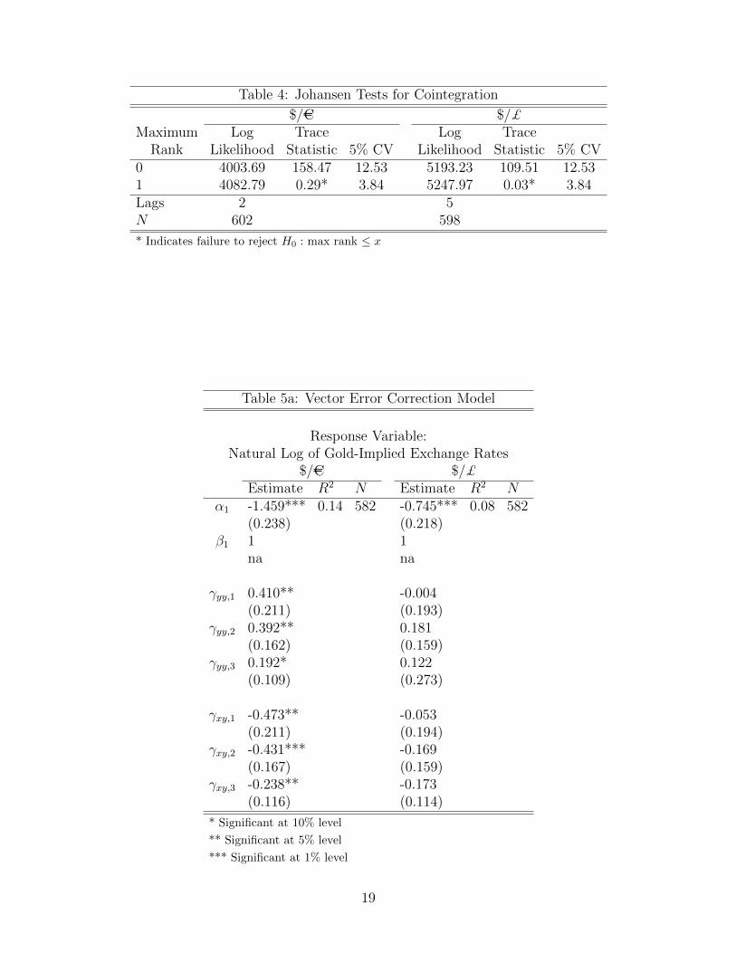
Table 4: Johansen Tests for Cointegration

$/AC $/£Maximum Log Trace Log Trace

Rank Likelihood Statistic 5% CV Likelihood Statistic 5% CV0 4003.69 158.47 12.53 5193.23 109.51 12.531 4082.79 0.29* 3.84 5247.97 0.03* 3.84Lags 2 5N 602 598

* Indicates failure to reject H0 : max rank ≤ x

Table 5a: Vector Error Correction Model

Response Variable:Natural Log of Gold-Implied Exchange Rates

$/AC $/£Estimate R2 N Estimate R2 N

α1 -1.459*** 0.14 582 -0.745*** 0.08 582(0.238) (0.218)

β1 1 1na na

γyy,1 0.410** -0.004(0.211) (0.193)

γyy,2 0.392** 0.181(0.162) (0.159)

γyy,3 0.192* 0.122(0.109) (0.273)

γxy,1 -0.473** -0.053(0.211) (0.194)

γxy,2 -0.431*** -0.169(0.167) (0.159)

γxy,3 -0.238** -0.173(0.116) (0.114)

* Significant at 10% level

** Significant at 5% level

*** Significant at 1% level

19

Table 5b: Vector Error Correction Model

Response Variable:Natural Log of Conventional Market Exchange Rates

$/AC $/£Estimate R2 N Estimate R2 N

α2 -0.448* 0.02 582 0.078 0.02 582(0.254) (0.218)

β2 -1.000*** -1.000***(0.000) (0.000)

γyx,1 0.498** 0.214(0.219) (0.209)

γyx,2 0.528*** 0.385**(0.173) (0.171)

γyx,3 0.233** 0.268**(0.116) (0.120)

γxx,1 -0.526** -0.236(0.225) (0.209)

γxx,2 -0.543*** -0.358**(0.178) (0.172)

γxx,3 -0.256** -0.288**(0.124) (0.123)

Significance of the Cointegrating Equation

$/AC $/£

χ2 1.40x107*** 3.51x107***

* Significant at 10% level

** Significant at 5% level

*** Significant at 1% level

20

Figure 1: Bitcoin Prices

Figure 2: Gold Prices

21

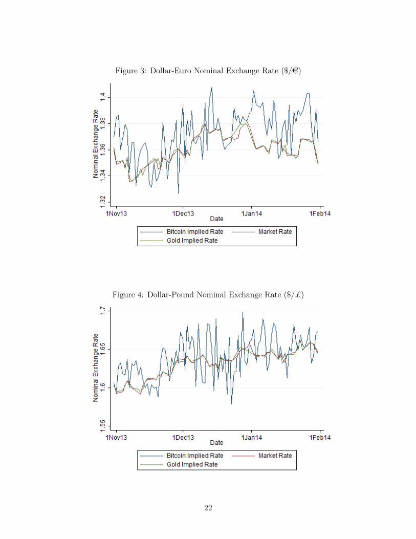
Figure 3: Dollar-Euro Nominal Exchange Rate ($/AC)

Figure 4: Dollar-Pound Nominal Exchange Rate ($/£)

22

Figure 5: Dollar-Australian Dollar Nominal Exchange Rate ($/A$)

Figure 6: Implied vs. Market Rate Spread for $/AC Rate

23

Figure 7: Implied vs. Market Rate Spread for $/£ Rate

Figure 8: Implied vs. Market Rate Spread for $/A$ Rate

24

Figure 9: Bitcoin Market-to-Implied IRF for $/AC Rate

Figure 10: Bitcoin Market-to-Implied IRF for $/£ Rate

25

Figure 11: Bitcoin Market-to-Implied IRF for $/A$ Rate

Figure 12: Bitcoin Implied-to-Market IRF for $/AC Rate

26

Figure 13: Bitcoin Implied-to-Market IRF for $/£ Rate

Figure 14: Bitcoin Implied-to-Market IRF for $/A$ Rate

27

Figure 15: Gold Market-to-Implied IRF for $/AC Rate

Figure 16: Gold Market-to-Implied IRF for $/£ Rate

28

Figure 17: Gold Implied-to-Market IRF for $/AC Rate

Figure 18: Gold Implied-to-Market IRF for $/£ Rate

29