
An Analysis of Approaches to Presence-Only Datahastie/TALKS/hastieSDM.pdf · An Analysis of...
94
An Analysis of Approaches to Presence-Only Data William Fithian and Trevor Hastie Department of Statistics Stanford University July 30, 2012
Transcript of An Analysis of Approaches to Presence-Only Datahastie/TALKS/hastieSDM.pdf · An Analysis of...
An Analysis of Approaches to Presence-OnlyData
William Fithian and Trevor HastieDepartment of Statistics
Stanford University
July 30, 2012

Species Distribution Modeling
Question: where may a given species be found?
Motivations:
• Plan wildlife management actions
• Monitor endangered or invasive species
• Scientific understanding
• etc.
What geographic features predict greater abundance?

Species Distribution Modeling
Question: where may a given species be found?
Motivations:
• Plan wildlife management actions
• Monitor endangered or invasive species
• Scientific understanding
• etc.
What geographic features predict greater abundance?
Species Distribution Modeling
Question: where may a given species be found?
Motivations:
• Plan wildlife management actions
• Monitor endangered or invasive species
• Scientific understanding
• etc.
What geographic features predict greater abundance?

Presence-Absence / Count Data
Scientists visit patch of land
Record whether any specimens encountered / how many
Relatively high quality data
Expensive, difficult for rare or elusive species
Presence-Absence / Count Data
Scientists visit patch of land
Record whether any specimens encountered / how many
Relatively high quality data
Expensive, difficult for rare or elusive species
Presence-Absence / Count Data
Scientists visit patch of land
Record whether any specimens encountered / how many
Relatively high quality data
Expensive, difficult for rare or elusive species

Presence-Absence / Count Data
Scientists visit patch of land
Record whether any specimens encountered / how many
Relatively high quality data
Expensive, difficult for rare or elusive species

Presence-Only Data
Motorist spies koala
Calls museum excitedly
Museum records location
Lower quality data
More of it exists
Increasingly popular object of study with advent of geographicinformation systems
Presence-Only Data
Motorist spies koala
Calls museum excitedly
Museum records location
Lower quality data
More of it exists
Increasingly popular object of study with advent of geographicinformation systems

Presence-Only Data
Motorist spies koala
Calls museum excitedly
Museum records location
Lower quality data
More of it exists
Increasingly popular object of study with advent of geographicinformation systems

Presence-Only Data
Motorist spies koala
Calls museum excitedly
Museum records location
Lower quality data
More of it exists
Increasingly popular object of study with advent of geographicinformation systems
Presence-Only Data
Motorist spies koala
Calls museum excitedly
Museum records location
Lower quality data
More of it exists
Increasingly popular object of study with advent of geographicinformation systems

Presence-Only Data
Motorist spies koala
Calls museum excitedly
Museum records location
Lower quality data
More of it exists
Increasingly popular object of study with advent of geographicinformation systems
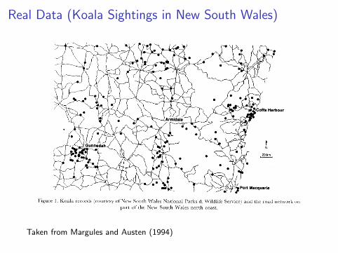
Real Data (Koala Sightings in New South Wales)
Taken from Margules and Austen (1994)

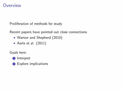
Overview
Proliferation of methods for study
Recent papers have pointed out close connections
• Warton and Shepherd (2010)
• Aarts et al. (2011)
Goals here:
1 Interpret
2 Explore implications
3 Extend results

Overview
Proliferation of methods for study
Recent papers have pointed out close connections
• Warton and Shepherd (2010)
• Aarts et al. (2011)
Goals here:
1 Interpret
2 Explore implications
3 Extend results

Overview
Proliferation of methods for study
Recent papers have pointed out close connections
• Warton and Shepherd (2010)
• Aarts et al. (2011)
Goals here:
1 Interpret
2 Explore implications
3 Extend results
Overview
Proliferation of methods for study
Recent papers have pointed out close connections
• Warton and Shepherd (2010)
• Aarts et al. (2011)
Goals here:
1 Interpret
2 Explore implications
3 Extend results
Overview
Proliferation of methods for study
Recent papers have pointed out close connections
• Warton and Shepherd (2010)
• Aarts et al. (2011)
Goals here:
1 Interpret
2 Explore implications
3 Extend results
Outline
1 Inhomogeneous Poisson Process Model / Maxent
2 Logistic Regression
3 Pooling Different Kinds of Data

Notation
n1 presence observations, n0 background observations
Geographic coordinates zi ∈ D ⊆ R2, i = 1, . . . , n0 + n1
Features xi = x(zi) measured via GIS
yi = 1 for presence, 0 for background

Notation
n1 presence observations, n0 background observations
Geographic coordinates zi ∈ D ⊆ R2, i = 1, . . . , n0 + n1
Features xi = x(zi) measured via GIS
yi = 1 for presence, 0 for background

Notation
n1 presence observations, n0 background observations
Geographic coordinates zi ∈ D ⊆ R2, i = 1, . . . , n0 + n1
Features xi = x(zi) measured via GIS
yi = 1 for presence, 0 for background

Notation
n1 presence observations, n0 background observations
Geographic coordinates zi ∈ D ⊆ R2, i = 1, . . . , n0 + n1
Features xi = x(zi) measured via GIS
yi = 1 for presence, 0 for background

Outline
1 Inhomogeneous Poisson Process Model / Maxent
2 Logistic Regression
3 Pooling Different Kinds of Data
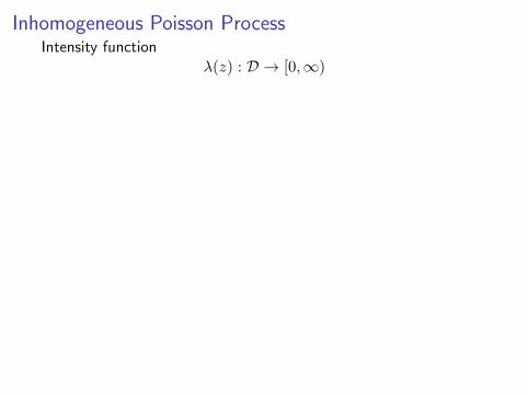
Inhomogeneous Poisson ProcessIntensity function
λ(z) : D → [0,∞)
Λ(A) =
∫Aλ(z) dz
Assume Λ(D) <∞.
pλ(z) = λ(z)/Λ(D)
Definition 1: choose poisson # points, then simple random sample
n1 ∼ Poisson(Λ(D))
zi|yi = 1i.i.d.∼ pλ
Definition 2: continuous limit of discrete poisson model
N(A) = #{i : zi ∈ A, yi = 1}∼ Poisson(Λ(A))
A ∩B = ∅ ⇒ N(A) ⊥⊥ N(B)
Presence-Only Data as IPP
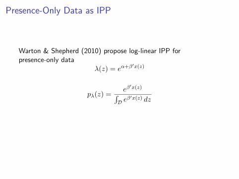
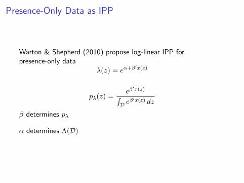
Warton & Shepherd (2010) propose log-linear IPP forpresence-only data
λ(z) = eα+β′x(z)
pλ(z) =eβ
′x(z)∫D e
β′x(z) dz
β determines pλ
α determines Λ(D)

Presence-Only Data as IPP
Warton & Shepherd (2010) propose log-linear IPP forpresence-only data
λ(z) = eα+β′x(z)
pλ(z) =eβ
′x(z)∫D e
β′x(z) dz
β determines pλ
α determines Λ(D)
Presence-Only Data as IPP
Warton & Shepherd (2010) propose log-linear IPP forpresence-only data
λ(z) = eα+β′x(z)
pλ(z) =eβ
′x(z)∫D e
β′x(z) dz
β determines pλ
α determines Λ(D)

Presence-Only Data as IPP
Warton & Shepherd (2010) propose log-linear IPP forpresence-only data
λ(z) = eα+β′x(z)
pλ(z) =eβ
′x(z)∫D e
β′x(z) dz
β determines pλ
α determines Λ(D)
Presence-Only Data as IPP
Warton & Shepherd (2010) propose log-linear IPP forpresence-only data
λ(z) = eα+β′x(z)
pλ(z) =eβ
′x(z)∫D e
β′x(z) dz
β determines pλ
α determines Λ(D)
Identifiability and Observer Bias
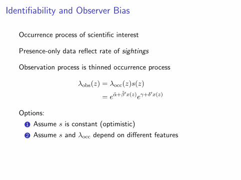
Occurrence process of scientific interest
Presence-only data reflect rate of sightings
Observation process is thinned occurrence process
λobs(z) = λocc(z)s(z)
= eα̃+β̃′x(z)eγ+δ
′x(z)
Options:
1 Assume s is constant (optimistic)
2 Assume s and λocc depend on different features
Either way, α̃ unidentifiable (α = γ + α̃)

Identifiability and Observer Bias
Occurrence process of scientific interest
Presence-only data reflect rate of sightings
Observation process is thinned occurrence process
λobs(z) = λocc(z)s(z)
= eα̃+β̃′x(z)eγ+δ
′x(z)
Options:
1 Assume s is constant (optimistic)
2 Assume s and λocc depend on different features
Either way, α̃ unidentifiable (α = γ + α̃)
Maximum Likelihood for IPP
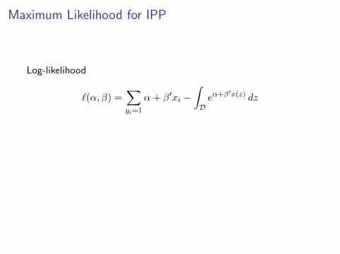
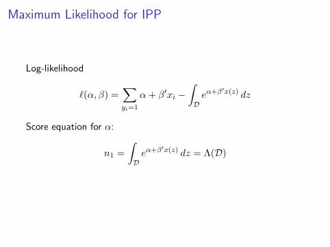
Log-likelihood
`(α, β) =∑yi=1
α+ β′xi −∫Deα+β
′x(z) dz
Score equation for α:
n1 =
∫Deα+β
′x(z) dz = Λ(D)
Implication: α̂ not of scientific interest unless n1 is
Maximum Likelihood for IPP
Log-likelihood
`(α, β) =∑yi=1
α+ β′xi −∫Deα+β
′x(z) dz
Score equation for α:
n1 =
∫Deα+β
′x(z) dz = Λ(D)
Implication: α̂ not of scientific interest unless n1 is

Maximum Likelihood for IPP
Log-likelihood
`(α, β) =∑yi=1
α+ β′xi −∫Deα+β
′x(z) dz
Score equation for α:
n1 =
∫Deα+β
′x(z) dz = Λ(D)
Implication: α̂ not of scientific interest unless n1 is
Maximum Likelihood for IPP
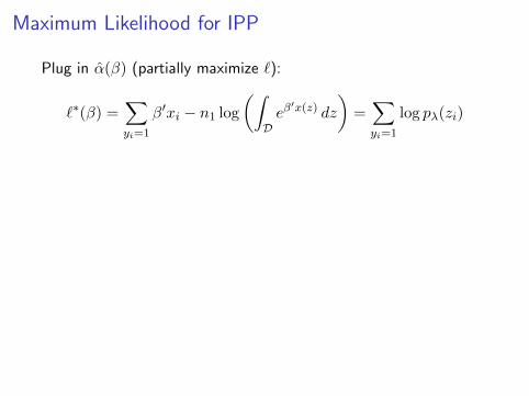
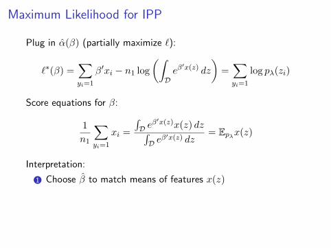
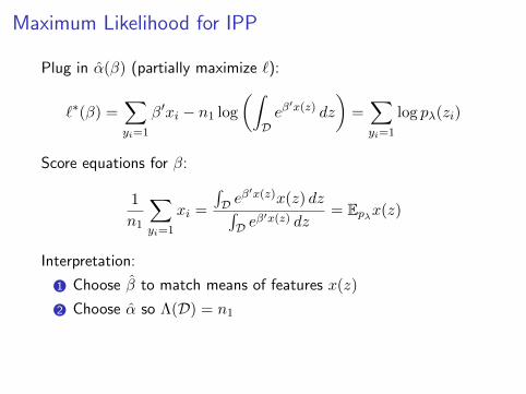
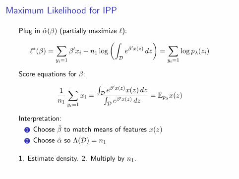
Plug in α̂(β) (partially maximize `):
`∗(β) =∑yi=1
β′xi − n1 log
(∫Deβ
′x(z) dz
)=∑yi=1
log pλ(zi)
Score equations for β:
1
n1
∑yi=1
xi =
∫D e
β′x(z)x(z) dz∫D e
β′x(z) dz= Epλx(z)
Interpretation:
1 Choose β̂ to match means of features x(z)
2 Choose α̂ so Λ(D) = n1
1. Estimate density. 2. Multiply by n1.

Maximum Likelihood for IPP
Plug in α̂(β) (partially maximize `):
`∗(β) =∑yi=1
β′xi − n1 log
(∫Deβ
′x(z) dz
)=∑yi=1
log pλ(zi)
Score equations for β:
1
n1
∑yi=1
xi =
∫D e
β′x(z)x(z) dz∫D e
β′x(z) dz= Epλx(z)
Interpretation:
1 Choose β̂ to match means of features x(z)
2 Choose α̂ so Λ(D) = n1
1. Estimate density. 2. Multiply by n1.

Maximum Likelihood for IPP
Plug in α̂(β) (partially maximize `):
`∗(β) =∑yi=1
β′xi − n1 log
(∫Deβ
′x(z) dz
)=∑yi=1
log pλ(zi)
Score equations for β:
1
n1
∑yi=1
xi =
∫D e
β′x(z)x(z) dz∫D e
β′x(z) dz= Epλx(z)
Interpretation:
1 Choose β̂ to match means of features x(z)
2 Choose α̂ so Λ(D) = n1
1. Estimate density.
2. Multiply by n1.
Maximum Likelihood for IPP
Plug in α̂(β) (partially maximize `):
`∗(β) =∑yi=1
β′xi − n1 log
(∫Deβ
′x(z) dz
)=∑yi=1
log pλ(zi)
Score equations for β:
1
n1
∑yi=1
xi =
∫D e
β′x(z)x(z) dz∫D e
β′x(z) dz= Epλx(z)
Interpretation:
1 Choose β̂ to match means of features x(z)
2 Choose α̂ so Λ(D) = n1
1. Estimate density. 2. Multiply by n1.
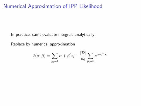
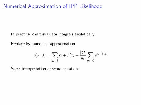
Numerical Approximation of IPP Likelihood
In practice, can’t evaluate integrals analytically
Replace by numerical approximation
`(α, β) =∑yi=1
α+ β′xi −|D|n0
∑yi=0
eα+β′xi
Same interpretation of score equations
Numerical Approximation of IPP Likelihood
In practice, can’t evaluate integrals analytically
Replace by numerical approximation
`(α, β) =∑yi=1
α+ β′xi −|D|n0
∑yi=0
eα+β′xi
Same interpretation of score equations
Numerical Approximation of IPP Likelihood
In practice, can’t evaluate integrals analytically
Replace by numerical approximation
`(α, β) =∑yi=1
α+ β′xi −|D|n0
∑yi=0
eα+β′xi
Same interpretation of score equations

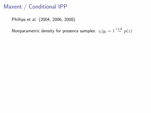
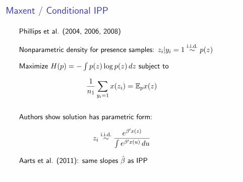
Maxent / Conditional IPP
Phillips et al. (2004, 2006, 2008)
Nonparametric density for presence samples: zi|yi = 1i.i.d.∼ p(z)
Maximize H(p) = −∫p(z) log p(z) dz subject to
1
n1
∑yi=1
x(zi) = Epx(z)
Authors show solution has parametric form:
zii.i.d.∼ eβ
′x(z)∫eβ′x(u) du
Aarts et al. (2011): same slopes β̂ as IPP

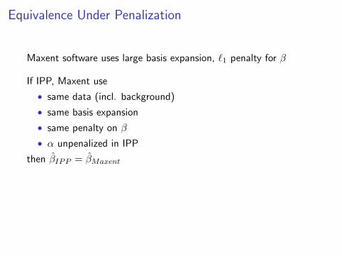
Equivalence Under Penalization
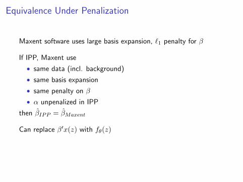
Maxent software uses large basis expansion, `1 penalty for β
If IPP, Maxent use
• same data (incl. background)
• same basis expansion
• same penalty on β
• α unpenalized in IPP
then β̂IPP = β̂Maxent
Can replace β′x(z) with fθ(z)
Same p̂(z), IPP also computes λ̂(z) = n1p̂(z)
Equivalence Under Penalization
Maxent software uses large basis expansion, `1 penalty for β
If IPP, Maxent use
• same data (incl. background)
• same basis expansion
• same penalty on β
• α unpenalized in IPP
then β̂IPP = β̂Maxent
Can replace β′x(z) with fθ(z)
Same p̂(z), IPP also computes λ̂(z) = n1p̂(z)
Outline
1 Inhomogeneous Poisson Process Model / Maxent
2 Logistic Regression
3 Pooling Different Kinds of Data

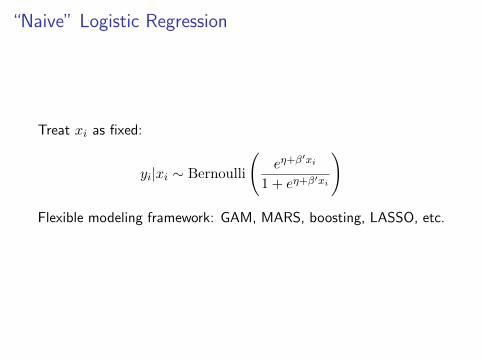
“Naive” Logistic Regression
Treat xi as fixed:
yi|xi ∼ Bernoulli
(eη+β
′xi
1 + eη+β′xi
)
Flexible modeling framework: GAM, MARS, boosting, LASSO, etc.
“Naive” Logistic Regression
Treat xi as fixed:
yi|xi ∼ Bernoulli
(eη+β
′xi
1 + eη+β′xi
)
Flexible modeling framework: GAM, MARS, boosting, LASSO, etc.

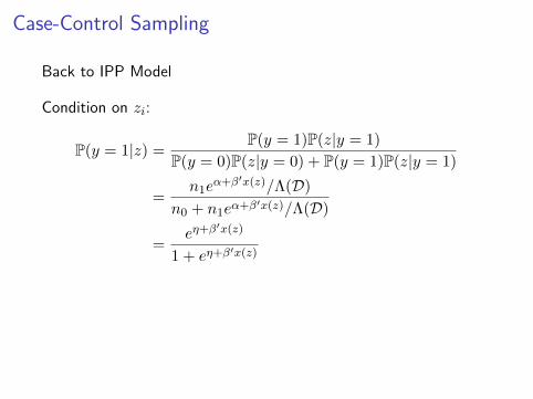
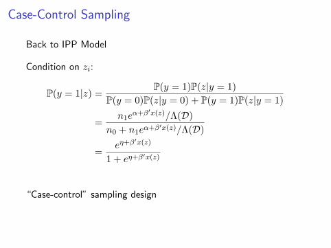
Case-Control Sampling
Back to IPP Model
Condition on zi:
P(y = 1|z) =P(y = 1)P(z|y = 1)
P(y = 0)P(z|y = 0) + P(y = 1)P(z|y = 1)
=n1e
α+β′x(z)/Λ(D)
n0 + n1eα+β′x(z)/Λ(D)
=eη+β
′x(z)
1 + eη+β′x(z)
“Case-control” sampling design
Logistic regression likelihood = conditional IPP likelihood
Case-Control Sampling
Back to IPP Model
Condition on zi:
P(y = 1|z) =P(y = 1)P(z|y = 1)
P(y = 0)P(z|y = 0) + P(y = 1)P(z|y = 1)
=n1e
α+β′x(z)/Λ(D)
n0 + n1eα+β′x(z)/Λ(D)
=eη+β
′x(z)
1 + eη+β′x(z)
“Case-control” sampling design
Logistic regression likelihood = conditional IPP likelihood
Case-Control Sampling
Back to IPP Model
Condition on zi:
P(y = 1|z) =P(y = 1)P(z|y = 1)
P(y = 0)P(z|y = 0) + P(y = 1)P(z|y = 1)
=n1e
α+β′x(z)/Λ(D)
n0 + n1eα+β′x(z)/Λ(D)
=eη+β
′x(z)
1 + eη+β′x(z)
“Case-control” sampling design
Logistic regression likelihood = conditional IPP likelihood

Case-Control Sampling
Back to IPP Model
Condition on zi:
P(y = 1|z) =P(y = 1)P(z|y = 1)
P(y = 0)P(z|y = 0) + P(y = 1)P(z|y = 1)
=n1e
α+β′x(z)/Λ(D)
n0 + n1eα+β′x(z)/Λ(D)
=eη+β
′x(z)
1 + eη+β′x(z)
“Case-control” sampling design
Logistic regression likelihood = conditional IPP likelihood

Logistic Regression vs IPP
Both estimate same β, but get different β̂
Warton & Shepherd (2010) show β̂LR → β̂IPP as n0 →∞ withn1 fixed
Misspecified case: not true if n0, n1 →∞ together (limit dependson limn1/n0)

Logistic Regression vs IPP
Both estimate same β, but get different β̂
Warton & Shepherd (2010) show β̂LR → β̂IPP as n0 →∞ withn1 fixed
Misspecified case: not true if n0, n1 →∞ together (limit dependson limn1/n0)

Logistic Regression vs IPP
Both estimate same β, but get different β̂
Warton & Shepherd (2010) show β̂LR → β̂IPP as n0 →∞ withn1 fixed
Misspecified case: not true if n0, n1 →∞ together (limit dependson limn1/n0)

Logistic Regression vs IPPFixed presence sample, n1 = 1000. True λ quadratic in x
●
●
100 1000 10000 1e+05 1e+06
0.0
0.2
0.4
0.6
0.8
1.0
1.2
Logistic Regression Estimates (n1 = 1000)
n0
β̂

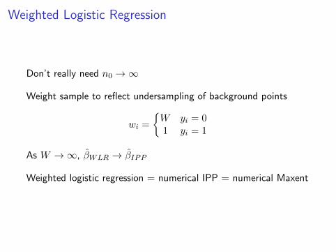
Weighted Logistic Regression
Don’t really need n0 →∞
Weight sample to reflect undersampling of background points
wi =
{W yi = 01 yi = 1
As W →∞, β̂WLR → β̂IPP
Weighted logistic regression = numerical IPP = numerical Maxent

Weighted Logistic Regression
Don’t really need n0 →∞
Weight sample to reflect undersampling of background points
wi =
{W yi = 01 yi = 1
As W →∞, β̂WLR → β̂IPP
Weighted logistic regression = numerical IPP = numerical Maxent

Weighted Logistic Regression
Don’t really need n0 →∞
Weight sample to reflect undersampling of background points
wi =
{W yi = 01 yi = 1
As W →∞, β̂WLR → β̂IPP
Weighted logistic regression = numerical IPP = numerical Maxent

Weighted Logistic Regression
Don’t really need n0 →∞
Weight sample to reflect undersampling of background points
wi =
{W yi = 01 yi = 1
As W →∞, β̂WLR → β̂IPP
Weighted logistic regression = numerical IPP = numerical Maxent
Weighted Logistic Regression
Don’t really need n0 →∞
Weight sample to reflect undersampling of background points
wi =
{W yi = 01 yi = 1
As W →∞, β̂WLR → β̂IPP
Weighted logistic regression = numerical IPP = numerical Maxent
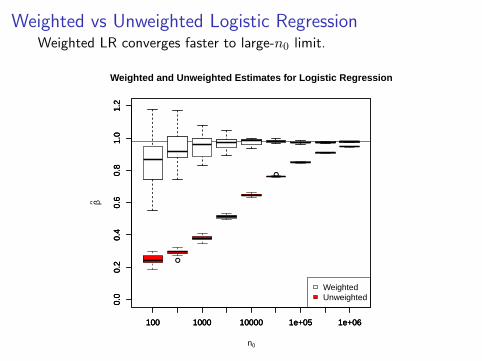
Weighted vs Unweighted Logistic RegressionWeighted LR converges faster to large-n0 limit.
100 1000 10000 1e+05 1e+06
0.0
0.2
0.4
0.6
0.8
1.0
1.2
Weighted and Unweighted Estimates for Logistic Regression
n0
β̂
●
●
100 1000 10000 1e+05 1e+06
0.0
0.2
0.4
0.6
0.8
1.0
1.2
100 1000 10000 1e+05 1e+06
0.0
0.2
0.4
0.6
0.8
1.0
1.2
WeightedUnweighted
Outline
1 Inhomogeneous Poisson Process Model / Maxent
2 Logistic Regression
3 Pooling Different Kinds of Data

Presence-Absence and Count Data
Implied likelihood for count / presence-absence data:
N |x ∼ Poisson(Aeα̃−ε+β̃
′x)
Can pool data from multiple studies

Presence-Absence and Count Data
Implied likelihood for count / presence-absence data:
N |x ∼ Poisson(Aeα̃−ε+β̃
′x)
Can pool data from multiple studies

Presence-Absence and Count Data
Implied likelihood for count / presence-absence data:
N |x ∼ Poisson(Aeα̃−ε+β̃
′x)
Can pool data from multiple studies
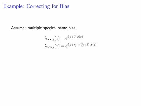
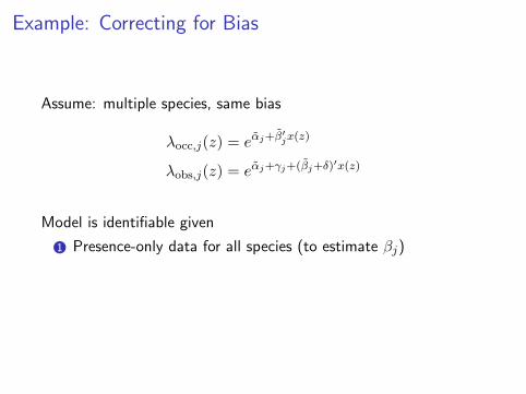
Example: Correcting for Bias
Assume: multiple species, same bias
λocc,j(z) = eα̃j+β̃′jx(z)
λobs,j(z) = eα̃j+γj+(β̃j+δ)′x(z)
Model is identifiable given
1 Presence-only data for all species (to estimate βj)
2 Presence-absence / count data for at least one species (toestimate δ)
Example: Correcting for Bias
Assume: multiple species, same bias
λocc,j(z) = eα̃j+β̃′jx(z)
λobs,j(z) = eα̃j+γj+(β̃j+δ)′x(z)
Model is identifiable given
1 Presence-only data for all species (to estimate βj)
2 Presence-absence / count data for at least one species (toestimate δ)

Example: Correcting for Bias
Assume: multiple species, same bias
λocc,j(z) = eα̃j+β̃′jx(z)
λobs,j(z) = eα̃j+γj+(β̃j+δ)′x(z)
Model is identifiable given
1 Presence-only data for all species (to estimate βj)
2 Presence-absence / count data for at least one species (toestimate δ)
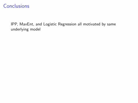
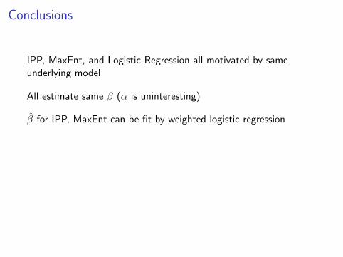
Conclusions
IPP, MaxEnt, and Logistic Regression all motivated by sameunderlying model
All estimate same β (α is uninteresting)
β̂ for IPP, MaxEnt can be fit by weighted logistic regression/ GAM/ Boosted Trees / MARS / Group LASSO / ...
boosted.ipp <- gbm(y~., family="bernoulli",
data=banksia, weights=1000^(1-y))
Can combine presence-only, presence-absence, and other data

Conclusions
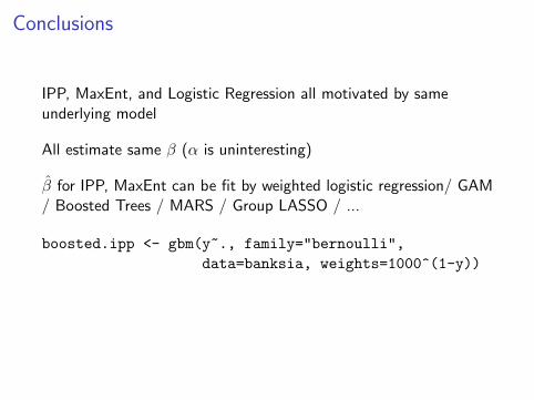
IPP, MaxEnt, and Logistic Regression all motivated by sameunderlying model
All estimate same β (α is uninteresting)
β̂ for IPP, MaxEnt can be fit by weighted logistic regression/ GAM/ Boosted Trees / MARS / Group LASSO / ...
boosted.ipp <- gbm(y~., family="bernoulli",
data=banksia, weights=1000^(1-y))
Can combine presence-only, presence-absence, and other data
Conclusions
IPP, MaxEnt, and Logistic Regression all motivated by sameunderlying model
All estimate same β (α is uninteresting)
β̂ for IPP, MaxEnt can be fit by weighted logistic regression
/ GAM/ Boosted Trees / MARS / Group LASSO / ...
boosted.ipp <- gbm(y~., family="bernoulli",
data=banksia, weights=1000^(1-y))
Can combine presence-only, presence-absence, and other data
Conclusions
IPP, MaxEnt, and Logistic Regression all motivated by sameunderlying model
All estimate same β (α is uninteresting)
β̂ for IPP, MaxEnt can be fit by weighted logistic regression/ GAM/ Boosted Trees / MARS / Group LASSO / ...
boosted.ipp <- gbm(y~., family="bernoulli",
data=banksia, weights=1000^(1-y))
Can combine presence-only, presence-absence, and other data
Conclusions
IPP, MaxEnt, and Logistic Regression all motivated by sameunderlying model
All estimate same β (α is uninteresting)
β̂ for IPP, MaxEnt can be fit by weighted logistic regression/ GAM/ Boosted Trees / MARS / Group LASSO / ...
boosted.ipp <- gbm(y~., family="bernoulli",
data=banksia, weights=1000^(1-y))
Can combine presence-only, presence-absence, and other data

Thanks