An analysis of a quasi-experiment in Zimbabwe INTRODUCTIONfafchamp/BarrDekkerFafchampsCBOs.pdf ·...

The formation of Community Based Organizations:

An analysis of a quasi-experiment in Zimbabwe

INTRODUCTION

Recent years have witnessed a renewed policy interest in community-based development

(Mansuri and Rao, 2004). This interest is predicated on the idea that community involvement in the

planning and execution of policy interventions leads to more effective and equitable development. In

practice, community-based interventions are often channelled through Community Based

Organizations (CBOs). In one critical respect this practice is well founded: CBOs often emerge and

play an important role in providing public goods and in resolving collective action problems when

formal institutions are deficient (Putnam 2000, Coleman 1988, Ostrom 1990). For this reason, they

are particularly important in poor countries where the government is unable or unwilling to provide

much needed social services, especially in rural areas (Edwards and Hulme 1995, Fafchamps 2006).

However, whether effective and equitable development can be achieved by assisting CBOs

ultimately depends on their composition and on where they do and do not emerge. If CBOs are

composed of local elites, interventions channelled through them are likely to reflect the preferences

and interests of those elites (Platteau and Gaspart 2003). Similarly, if CBOs form along gender or

ethnic lines, their mode of operation is likely to reflect the interests of specific gender or ethnic

groups rather than the interests of the community as a whole. More generally, if existing socio-

economic cleavages are reflected in the composition of CBOs (by exclusion of individuals who do not

have certain characteristics or through segmentation) this may negatively affect social cohesion and

solidarity (De Bock, 2014). Finally, if CBOs tend not to emerge in the poorest communities, then

communities in greatest need of assistance could miss out on important development opportunities.

An understanding of the emergence and composition of CBOs is thus of major policy interest.

Arcand and Fafchamps (2012) investigate CBO membership and co-membership, i.e., who is

linked to whom as a result of belonging to the same CBOs in Senegal and Burkina Faso. They find

that more prosperous members of rural society are more likely to belong to CBOs and that members

2

of ethnic groups that traditionally focus on raising livestock rather than on crop cultivation are less

likely to belong to CBOs. They also find that CBO membership is assortative on wealth and ethnicity,

i.e., that the wealthy tend to group with the wealthy and the poor with the poor, and that different

ethnic groups tend not to group together. These are the sort of group formation patterns that ought to

be of potential concern for development practitioners.

In common with a large literature on the role of social networks in risk and information

sharing within agrarian communities of Africa (e.g, De Weerdt, 2004; Dekker, 2004; Udry and

Conley, 2004; Fafchamps and Gubert, 2006; Krishnan and Sciubba, 2009; De Bock, 2014), Arcand

and Fafchamps (2012) rely on cross-section data. This literature provides vital descriptive information

on group composition, but cannot always satisfactorily address issues of causality. Specifically, it

cannot always tell whether similarities cause people to associate with one another or whether

association causes people to become more similar.i The issue of reverse causation does not arise for

gender or ethnicity since these are, in principle, immutable. But when the characteristics of interest

are income, wealth, and prosperity broadly defined, causal ambiguity needs to be resolved.

Furthermore, cross-section data does not facilitate the identification of causal effects running from

community composition to CBO formation, an issue that arises both for mutable characteristics such

as wealth as well as, via selection effects, for immutable individual characteristics such as gender and

ethnicity.

In this paper, we obviate these concerns by focusing on data from a de facto quasi-experiment

resulting from actions taken over a quarter of a century ago by the, then, newly formed Zimbabwean

government. After the Zimbabwean war of independence in 1980, many people displaced by the

fighting were resettled in newly created villages. These resettled villages were created by government

officials selecting households from lists of applicantsii. Thus, unlike traditional villages that are

organized along kinship lines, these new villages brought together households that were typically

unacquainted with each other, often of different lineage and diverse in terms of wealth (Dekker,

2004).iii Yet, in order to survive and prosper, the inhabitants of these newly created villages had to

3

solve various collective action problems relating to natural resource management, risk management,

indivisibilities in inputs to agrarian production, and inadequate access to financial and other services.

The creation of new villages with households selected at random forms a quasi-experiment that offers

a unique opportunity to study the community formation process.iv

The nature of the quasi-experiment is similar to the random assignment of roommates to

dorms or classes studied by Sacerdote (2001) and others (e.g., Lyle 2007, Shue 2012) or to the

random assignment of entrepreneurs to judging committees engineered by Fafchamps and Quinn

(2012). The difference is that we do not use random assignment to study peer effects but rather to

study assorting and group formation between people who have been randomly brought together.

Perhaps the closest analogy to what we do is the Big Brother TV show: people from different

backgrounds are thrown together into the House, and viewers study the friendships and cliques they

form over time. In this case, the government of Zimbabwe grouped previously unassociated

households together in new villages and we study the CBOs those households form over time.

We show that, to varying degrees, the fifteen studied villages addressed collective action

problems by setting up CBOs. We investigate CBO formation using data on the geography of the

newly formed villages, kinship and lineage networks between resettled households, and the

characteristics of the households at the time of their resettlement. We focus our analysis on two

specific questions – who groups and who groups with whom – using only household characteristics at

the time of resettlement. We investigate for how long these characteristics affect CBO formation and

co-membership over time. We focus our analysis on CBOs that have an economic – as opposed to

purely social – purpose. Earlier analysis (Barr et al, 2012) shows that co-memberships in these CBOs

are more predictive of group formation in incentivized lab-type experiments, suggesting that, relative

to other co-memberships, they are stronger and probably more valuable.

We make use of a unique dataset combining information from multiple sources: a panel

survey of households that ran from 1983 to 2000; detailed retrospective data on CBO membership

collected in 2000; genealogical data collected in 1999 and 2001; lineage data collected in 2001 and

4

2009; and village geography data collected in 1999 and 2009. Merging, completing, and reconciling

(to the extent possible) these datasets took many months of work by the authors and researchers in

the field in Zimbabwe. To our knowledge this is the first dataset on small farming communities that

combines detailed information on socio-economic characteristics with a wide range of intra-village

social ties over such a long period of time.

The analysis reveals that the studied communities do not appear to be elitist. We find that, by

the end of 1982, at a time when almost 90 percent of sampled households had settled in the new

villages, wealthier households had already formed CBOs to serve a variety of economic purposes.

Poorer households initially tended not to engage in CBOs but, by 1983, this difference had

disappeared. Wealthier households may have been the ones who initiated CBOs because clearing

land, planting crops, and building houses on uninhabited land proved easier for them. What is

remarkable is that poorer households were allowed to join without apparent prejudice as and when

their circumstances allowed.

The analysis further shows that the network of CBO co-memberships is denser in poorer

villages. Why this is the case is not entirely clear. One possibility is that they had a greater need to

organize in order to address indivisibilities in agrarian inputs and to cope with risk. This pattern

persists throughout the eighteen post-resettlement years covered by our dataset. In addition, we find

strong evidence against the separation of female and male headed households into different CBOs.

There is, however, some evidence that the female-headed households are involved in fewer CBOs.

Cause for concern is raised only by evidence that those who settled early and those who settled late

associate less with one another than those who settled at the same time. There is also weak evidence

that non-Zimbabwean households are less engaged in CBO activities. Within these small resettled

villages, geographical proximity affects CBO co-membership only in early years: by 1985 we observe

no affect of proximity on who groups with whom. The effect of kinship on co-membership is similarly

occasional and ephemeral. Shared lineage has no bearing on co-membership, although, at the

community level, we find evidence that shared lineage and CBO activity are substitutes.

5

Since households in our dataset generally had little to no interaction with one another before

they came to the new villages, these findings can be fairly safely given a causal interpretation. But there

is a downside: given their artificial creation process, the study villages are not representative of

developing-country villages in general or even of Zimbabwean villages. This limitation of the study

needs to be born in mind when considering the external validity of our findings. It should be noted,

however, that new communities made up of displaced people are not uncommon in the developing

world, especially in post-conflict situations. In this context, findings such as ours are both rare and of

potential value to development practitioners.

The remainder of the paper is organized as follows. In section 2 we introduce various

hypotheses of interest regarding CBO formation in resettled villages, and we propose an empirical

model that distinguishes between them. In this model co-membership in CBOs is a function of

geographical, social, and economic proximity. In section 3 we describe our data sources in detail. In

section 4 we present descriptive statistics regarding the evolution of CBO co-memberships between

1980 and 2000 in each of the fifteen villages in our sample. In section 5 we present estimation results

for an extensive series of regressions corresponding to the specification presented in section 2. In

section 6 we present a circumspect (owing to the fact that there are only fifteen villages in our sample)

but nevertheless informative analysis of CBO co-membership at the village-level. In section 7, we

return to the dyadic analysis armed with new insights from the village-level analysis and we investigate

what happens when we divide the sample according to one specific, village-level characteristic. Finally,

in section 8 we discuss our findings and consider why they differ from those of Arcand and

Fafchamps (2012) and what this implies for the generality of each study’s findings.

ANALYTICAL FRAMEWORK AND EMPIRICAL SPECIFICATION

CBOs provide a basis for collective action, in part, because they allow trust between individual

members to develop. Trust can have different origins. It may arise from a shared lineage or kin

6

group, but we expect this source of trust to be less important in our study villages, given the way they

were formed. Another possible source, common to all households in our study, is the prospect of a

future in close proximity with one another. This prospect would generate a need for each person to

develop and maintain a reputation of trustworthiness that, combined with self-interest, may be

sufficient to support trust and reciprocation. This hypothesis was articulated by Posner (1980) and

subsequently formalized by Coate and Ravallion (1993).

Households differ in the cost of joining a CBO, and in the benefits they can hope to derive.

We therefore expect some differentiation across households in terms of CBO membership. First, as

pointed out by Arcand and Fafchamps (2012) and others before them, pre-existing kinship ties and

shared lineage may favour trust-reinforcing altruism.v Second, similarity in socio-economic

characteristics such as age, household composition, or wealth may reduce the costs of developing an

acquaintance on which trust and more valuable forms of association can be built. Third, physical

proximity increases the frequency of chance encounters and reduces the costs of maintaining regular

contact. Fourth, a households’ early arrival in the village may create a shared sense of pioneering

camaraderie, resulting in a feeling of entitlement and responsibility in village affairs. With the arrival

of additional households, these feelings may have turned into resentment towards latecomers who

brought additional pressure on shared resources and could free ride on collective actions initiated

prior to their arrival.

Turning to the benefits of setting up CBOs, these too vary across households and villages. We

expect poorer households to find indivisibilities in agricultural inputs harder to overcome on their

own. For example, a rich household could afford a ploughing pair of oxen. But a less fortunate one

could only afford a ploughing pair by sacrificing consumption and a poor household could not afford

one on their own. We also expect poorer households to have a greater need for informal insurance

via risk pooling. We therefore expect rich and poor households to have different interests in CBOs.

The benefits associated with setting up CBOs also depend on whether alternative mechanisms

exist for addressing collective problems. Forming a CBO signals commitment to a common cause.

7

Membership fees (in money or in kind) can act as a material pre-commitment to that cause. However,

collective agreements can also be enforced via kin- or lineage-based mechanisms involving well-

established behavioural norms enforced through lateral and hierarchical pressure. For kin- and

lineage-based mechanisms to facilitate collective action in the resettled villages, the kin or lineage

network must be sufficiently dense. Since settlers were rarely settled with their close kinfolk, this is

unlikely to have played an important role in our study villages. However, authorities tended to assign

to a new village those settlers coming from the surrounding areas. Hence the lineage network may

have been sufficiently dense in some villages. Working with a cross-section of the data used here

along with data from six traditional villages, Barr (2004) found less CBO membership in villages with

denser lineage networks. This is consistent with CBOs and lineage networks being substitute bases in

the provision of local public goods.

The various hypotheses described above can all be captured within a dyadic model of link

formation of the form proposed by Fafchamps and Gubert (2007) and Arcand and Fafchamps

(2012). The model takes the general form 𝑚!" = 𝜆(𝑥!") where 𝑚!" is the number of CBO co-

memberships that i and j share. Function 𝜆 . depends on a vector 𝑥!" that includes factors that affect

the number and size of the groups that i and j belong to, and factors that affect the likelihood that i

and j belong to the same group. More about this later.

When estimating a dyadic regression, the main technical difficulty is to obtain consistent

standard errors owing to interdependence across 𝑚!"s. This interdependence could tempt one into

estimating a joint maximum likelihood function. There are several problems with this approach,

however. First, estimation requires solving a complicated optimization problem with multiple

integrals. This can, in principle, be achieved – e.g., using the Gibbs algorithm – but at a non-negligible

cost in terms of programming. Second and more importantly, writing down the joint likelihood

function forces the researcher to specify the functional form of the interaction between observations.

Theoretically, this can improve efficiency, but it can also result in inconsistent estimates if the

specified form of interaction is wrong. So, we opt for one of the simpler and more transparent

8

approaches applied to analyses of this type. Among these approaches, the most extensively used are

the quadratic assignment permutation method (QAP), developed by Krackhardt (1987), and the

dyadic robust standard error regression approach developed by Fafchamps and Gubert (2007).vi We

use the latter primarily because it easily allows pooling data across disjoint populations.

The estimation of dyadic models requires some care regarding the way regressors are

incorporated (Fafchamps and Gubert; 2007). In our case, the network matrix 𝑀 = [𝑚!"] is

symmetrical: if i belongs to the same CBO(s) as j, by construction j also belongs to the same CBO(s)

as i, i.e., 𝑚!" = 𝑚!". To ensure that 𝐸 𝑚!" = 𝐸 𝑚!" regressors must enter the model in a symmetric

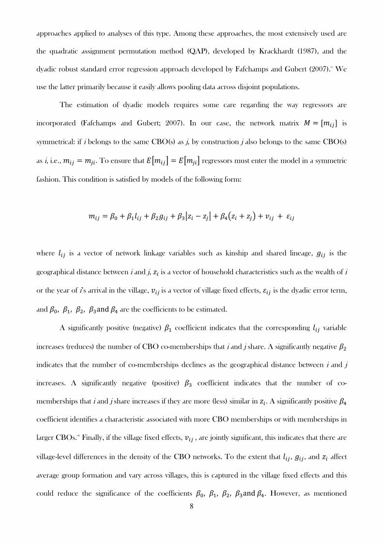
fashion. This condition is satisfied by models of the following form:

𝑚!" = 𝛽! + 𝛽!𝑙!" + 𝛽!𝑔!" + 𝛽! 𝑧! − 𝑧! + 𝛽! 𝑧! + 𝑧! + 𝑣!" + 𝜀!"

where 𝑙!" is a vector of network linkage variables such as kinship and shared lineage, 𝑔!" is the

geographical distance between i and j, 𝑧! is a vector of household characteristics such as the wealth of i

or the year of i’s arrival in the village, 𝑣!" is a vector of village fixed effects, 𝜀!" is the dyadic error term,

and 𝛽!, 𝛽!, 𝛽!, 𝛽!and 𝛽! are the coefficients to be estimated.

A significantly positive (negative) 𝛽! coefficient indicates that the corresponding 𝑙!" variable

increases (reduces) the number of CBO co-memberships that i and j share. A significantly negative 𝛽!

indicates that the number of co-memberships declines as the geographical distance between i and j

increases. A significantly negative (positive) 𝛽! coefficient indicates that the number of co-

memberships that i and j share increases if they are more (less) similar in 𝑧!. A significantly positive 𝛽!

coefficient identifies a characteristic associated with more CBO memberships or with memberships in

larger CBOs.vii Finally, if the village fixed effects, 𝑣!" , are jointly significant, this indicates that there are

village-level differences in the density of the CBO networks. To the extent that 𝑙!", 𝑔!", and 𝑧! affect

average group formation and vary across villages, this is captured in the village fixed effects and this

could reduce the significance of the coefficients 𝛽!, 𝛽!, 𝛽!, 𝛽!and 𝛽!. However, as mentioned

9

above when discussing the role of lineage, there is no a priori reason to expect a particular regressor

to have a similar effect at the dyad and village level. In this case, the inclusion of the village fixed

effects can improve efficiency and increase the significance of the coefficients 𝛽!, 𝛽!, 𝛽!, 𝛽!and 𝛽!.

The analysis involves the estimation of a series of dyadic models using 𝑚!" as the dependent

variable. We also estimate an alternative linear probability model using 𝑑!" = 1 if 𝑚!" > 0 and = 0 if

𝑚!" = 0 as the dependent variable.viii We estimate these two models for each year for which we have

relevant data, that is, starting with 1982 when village settlement is nearly complete, and ending with

2000 when insecurity in Zimbabwe forced us to stop data collection. In all cases, the regressors relate

to the dyadic baseline. This is the point in time when both households in the dyad are resettled –

typically a year between 1980 and 1984. Regressors are described in detail in the next sections.

We also conduct a series of village-level linear regressions, one for each year. Given the small

number of observations – there are only 15 villages in our dataset – this raises doubts regarding the

power of our analysis. In spite of this shortcoming, one important effect is nonetheless confirmed.

DATA SOURCES, SAMPLES AND DEFINITIONS

In 1980, the Government of Zimbabwe aimed at resettling 18.000 displaced households over

a period of five years. By March 1982, 12 schemes accommodating 5070 settler families had been

established (Kinsey, 1982) and by 1989 a total of 52000 families had been relocated (Palmer, 1990).

In this paper we use data on 15 randomly selected villages from 2 of the 12 schemes that were

established by March 1982.ix The two schemes differ from one another in terms of suitability for

agriculture.x One of the two selected schemes is comparable to 2 of the schemes established in the

same period, while the second is comparable to 6 other schemes. The remaining 4 schemes are

situated in environments less suitable for crop production (Kinsey, 1982) and are not included in our

analysis.

10

Resettled households started to arrive in the fifteen sample villages in 1980 (see Table 1). The

inflow peaked in 1981 and almost 90 percent of sample households had settled by the end of 1982.

After 1982 the household composition of each village stabilized. There were a few more arrivals –

generally people who applied for resettlement in 1980 but had not been allocated land immediately.

There were very few departures. When a household head died during the study period, their farm

typically passed to members of their family, either to their surviving wife or to one of their sons. Heirs

inherited the right to farm the fields, to use common grazing lands, and to reside in the family

homestead. We treat these cases as the survival of a dynastic household. In our data a household is

regarded as having left when the family vacated land and homestead, either following the death of a

household head or for some other reason. There are 504 households in the dataset with at most 499

appearing in the villages at any one time. Village size varies. The smallest village only has thirteen

households throughout most of the time period covered by our data. The largest reached a maximum

of 52 households in 1998.

[Table 1 approximately here]

The data we use for the analysis in this paper combines information on the same households

from multiple sources. The socio-economic variables are drawn from the Zimbabwe Rural

Household Dynamics Study (ZRHDS). The ZRHDS started in March 1983 and aimed to include all

the households present in our study villages at that time.xi From the first round of the ZRHDS we

extract data on: livestock holdings upon arrival in the village; the age, sex and education of the

household head; the headcount size of each household upon arrival; and whether the household

resided in a village placed under curfew by the UDI government during the war. We regard this last

variable as a rough proxy for the intensity of fighting in the household’s previous place of residence.

In Zimbabwe, livestock is kept as a store of wealth and a productive asset and sometimes as part of a

mixed farming system. We therefore use livestock holdings as indicator of initial wealth. Livestock is

11

measured in oxen-equivalent, with weights for different categories of animals constructed from 1995

market prices.

Subsequent survey rounds conducted between 1987 and 2000 revisited the households

interviewed in 1983. xii As a result, they do not include the late arrivals. These were identified and

surveyed by us in 1999, in a single comprehensive survey round in which respondents were asked to

recall the time of their arrival in the village and some of the characteristics of their households at that

time.

Table 2 summarizes the characteristics and livestock holdings on arrival of the household

heads residing in the study villages in 1980, 1982, and 1984.xiii The average livestock holdings at the

time of resettlement were 3.2 – equivalent to a pair of oxen, one milking cow, and a few chickens. 38

percent of households arrived with no livestock at all. They would have faced the prospect of clearing

land and cultivating at least a first set of crops without a ploughing pair of their own.xiv The age of the

average household head in 1980 was 38 years. Later arrivals tended to be a little older. The average

household size was between five and six members in 1980. Figures for subsequent years indicate

either that late arrivals had larger households or that households expanded after resettlement through

procreation or in-migration.


Data on CBOs were collected in 2000 during a six-week period of intensive fieldwork

involving Barr and a small team of field researchers (see Barr, 2004).xv The objective was to collect

comprehensive data on civil social activity at the time and in the preceding two decades. Considerable

thought went into designing a fieldwork protocol to maximize data quality. Using the Local Level

Institutions Study (World Bank, 1998) as template, we designed a data-generating protocol with two

main components.xvi The first component involved a village meeting attended by one adult member of

every household in the village (a small number of households were unable to attend). During this

12

meeting, a list was drawn of all the non-political groups that had ever existed in the village or to which

village members had belonged. This list includes clubs, religious groups, unions, rotating savings and

credit associations, and funeral societies.xvii One field researcher led the discussion among villagers

while others wrote independent lists of the groups mentioned in the discussion. A master list was then

assembled and presented to villagers at the meeting. It was further corroborated by researchers who

engaged villagers in side conversations to collect any additional relevant information. From this

process, we constructed an exhaustive list of groups that either existed at the time of the meeting or

had existed at some time during the history of the village.

These lists became the code sheet for the next stage of data collection, which involved the

recording of individual household’s civil social histories. To ensure that the recall is as accurate as

possible, we did not interview household representatives in isolation but instead constructed a panel

of informants for each household. These panels usually include neighbours as well as household

members. To reduce time pressure, panel interviews took place while refreshments were being served

at the end of village meetings relating to other research tasks, or while menial tasks such as shelling

groundnuts or beans were undertaken by groups of neighbours. This approach proved particularly

valuable when the original settler had died, leaving behind family members too young to remember

the early years of the household’s history. This approach also allowed us to construct histories for the

few households that no longer resided in the villages.

Generally, we find that women in their 40s and 50s were the most reliable panel members.

Men recalled male activity with a high degree of accuracy, but provided inaccurate data on the current

and past civil social activity of female household members. The existence of a “year zero”, i.e., a point

in time when the village was created ad nihilo and before which there was no civil society, provided an

important anchor for the recall exercise. Natural dating techniques, principally involving references to

drought years such as 1992 and 1995, were also used. As a result we have what we believe is a fairly

complete year-by-year network of civil social activity in each village.

13

Protocol details notwithstanding, it is important to bear in mind that we were asking

respondents to recall events during the preceding two decades – in some cases not just for themselves

but also for absent others. The analysis presented below thus should be viewed as jointly testing the

hypotheses outlined above and the accuracy of the data collection. In general we expect recall errors

to introduce noise and reduce power. The only reason why recall errors may lead to spurious

inference is if respondents fill gaps in their memory with guesses based on a shared theory. The

likelihood of such occurrence appears slim, however. Recall error is far more likely to inflate standard

errors and the estimates presented below should be regarded as conservative.

Table A1 provides a breakdown of all the CBOs in the dataset, by village and starting date.

The majority of the CBOs, 70 percent, have members from the village only and less than a quarter of

the reported CBOs have connections to external agents such as NGOs or government. Our analysis

focuses on co-memberships in CBOs serving an economic purpose. These represent 41 percent of

the CBOs listed in the fifteen villages. They include funeral societies, ROSCAs, and a diverse range

of agricultural and other income generating cooperatives aiming to maintain collectively owned

indivisible structures and to harness economies of scale. They also include activities to learn and share

new skills, most often relating to adult literacy or agricultural practices.xviii

CBOs serving a purely social purpose, such as choirs, dance groups, and football and netball

clubs represent 15 percent of the listed CBOs. Tests indicate that recall data on these organizations

are of considerably poorer quality, suggesting that membership is less important and thus harder to

recall. To the extent that the data can be analysed at all, social CBOs appear to follow a different

formation process. It is therefore safer to omit them from the analysis.xix We also exclude religious

organizations, as religious affiliation is likely to predate resettlement.xx Unfortunately, no information

was collected on religious affiliation at the time of resettlement, so we cannot control for it.

Religiousgroups represent 44% of the listed CBOs.

Each questionnaire used to collect CBO membership data started with the question “Has

anyone from this household ever regularly attended the meetings of [the name of a group or

14

association]?” This was followed by a series of questions about who attended, when the first attendee

started attending, and when the last attendee stopped attending. Questions were also asked about

attendance rates, contributions, and leadership. The precise identity of the attendees was not

collected; we only know whether the attendees included the head of household, an adult male or

female, or a male or female child. When several members attended, we do not know who was first

and last. This protocol rules out studying individual connectedness.xxi To the extent that CBO

membership and attendance decisions are taken jointly by the household, household

interconnectedness is probably a better unit of analysis anyway. For the remainder of the paper 𝑚!"

denotes the number of economic CBOs in which households i and j have at least one member each.

Similarly, 𝑑!" is set to one when at least one member of household i and one member of household j

belong to the same CBO.

The data on kinship were collected in 1999 and 2001. A specifically designed social mapping

exercise was conducted using village focus groups involving at least one representative from each

household residing in each village (Dekker 2004). Information was obtained about the years of

settlement, marriage, divorce and death necessary to construct a panel of kinship ties. This

information was then combined with marriage and household roster information from the panel

survey and with a death registry collected separately in 2000 (see Barr and Stein, 2008). The help of

experienced field researchers was enlisted in 2009 to complete missing information using natural

dating techniques.

In the analysis, the relatedness of households i and j is defined as the maximum Hamilton’s

ratio between any member of household i and any member of household j. Hamilton’s ratio is a

measure of genetic relatedness. Marriage relations are captured as well. In accordance with local

tradition, if the daughter of household i marries an adult male in household j, she moves into that

household. Being related to her father and mother in household i, the Hamilton’s ratio between the

two households equals 0.5, which is its maximum possible value assuming no inbreeding. Although a

full panel of kinship ties is available, here we only use initial relatedness, e.g., the kinship ties between

15

two households in the year of settlement.xxii In the case of inter-marriage, the Hamilton’s ratio between

i and j equals 0.5 if the marriage took place before the two households had settled in the village.

The lineage data was collected in nine of the villages in 2001 and in the remaining six in 2009.

Following consultations with experienced local field researchers, we chose to collect data on the totem

of each household head and their spouse(s). In the study area, someone’s totem is made of three

elements: their Mutupo, Chidao and Dzinza. These terms refer to the patrilineal clan, subclan and

subsection of the subclan, respectively. Both Mutupo and Chidao have religious and symbolic

connotations. Someone’s Dzinza simply traces their family roots and refers to the fourth male

ancestor up the family tree (Bourdillon, 1976). It also indicates the geographical location of the clan

lands upon which an individual’s great-grand parents lived. In the analysis below, we use the Dzinza as

a lineage variable. More specifically, household i is defined as having a shared lineage with household

j if household i’s head’s or spouses’ Dzinza matches household j’s head’s or spouses’ Dzinza. This

captures co-membership in a broad family network. Given the lack of close kinship ties in the

resettled villages, this broad family network could provide a sense of shared identity and facilitate the

provision of hospitality and support (Stead, 1946, Spierenburg, 2003). This exercise also revealed that

almost seven percent of the sampled households are of non-Zimbabwean origin.

For nine of the villages, we had geographical maps sketched in 1999 as part of the kinship

mapping exercises. Originally, they were not intended to act as a source of geographical data. But,

when we began work on this project in 2009, we returned to the maps as a source of geographical

proximity data. We approximated scale of each map using information about the size of the

homestead plots officially assigned to each household. Having established that this exercise yielded

useable data, we dispatched a small team of local researchers to draw similar sketch maps in the

remaining six villages. They also measured a few key distances to verify the accuracy of our

approximation of the scale of each map. In the analysis presented below, we use the estimated

distance in Km between each pair of households as a measure of the geographical distance between

them.

16

The following regressors are used in the dyadic regression analysis:

o The difference between household i’s livestock holding at the time when it settled, and

household j’s livestock holding at the time when it settled

o The sum of livestock holdings at settlement

o A dummy equal to 1 if one household is female headed and the other is not, 0 otherwise

o The number female headed households

o The difference between the ages of the heads of households i and j at the time of settlementxxiii

o The sum of the ages of the household heads

o A dummy equal to 1 if one household is non-Zimbabwean, the other not; 0 otherwise

o The number non-Zimbabwean households

o A dummy equal 1 1 if one household previously lived in a curfew village, the other not

o The number of households that previously lived in a curfew village

o The difference in settlement date (in years) between households i and j

o The sum of i and j’s settlement dates, each measured in years since the start of the

resettlement programme, i.e., 1980=0, 1981=1, etc.

o The difference in the size (head count) of households i and j at time of settlement

o The sum of the sizes of households i and j at the time of settlement

o The genetic relatedness between the two households, defined as the maximum Hamilton’s

ratio between all possible matched pairs of individuals from household i and j at time of

settlement

o A dummy equal to 1 if the two households have a shared lineage or Dzinza

o The estimated distance in Km between the homesteads of households i and j

We realize that, in general, the building of new kinship ties through marriage may be an important

predictor of co-membership in CBOs. In our data, there were no such ties across households at the

time of resettlement. All marriage ties across study households occurred after resettlement and are

potentially endogenous to the CBO formation process we study, e.g., people may marry someone

17

they meet at CBO events. Hence conditioning on marriage ties across households could introduce

reverse causation in the analysis. This is the reason why we do not include marriage ties in the

analysis.

DESCRIPTIVE STATISTICS

Across the fifteen villages in our dataset there are 127 different economic CBOs. In any given

year, a CBO in existence in that year includes members from 13 to 15 households. Table 3

summarizes, year by year, the network of co-memberships defined by these 127 CBOs for the full

sample of within-village household dyads, and for the regression sample for which we have complete

data to estimate dyadic regressions. For these two samples the Table reports sample size in each year,

the percentage of dyads that share at least one CBO co-membership, and the average number of

CBO co-memberships shared by a dyad.


We note a steady rise in CBO co-membership over time. In 1983, 58 percent of the

household dyads shared at least one CBO co-membership. By 2000 that figure had risen to 84

percent. Over the same period the average number of co-memberships increased from just under one

to just under two. There is no discernible difference between the full sample and the regression

sample. These numbers are consistent with a high level of CBO activity and a high degree of

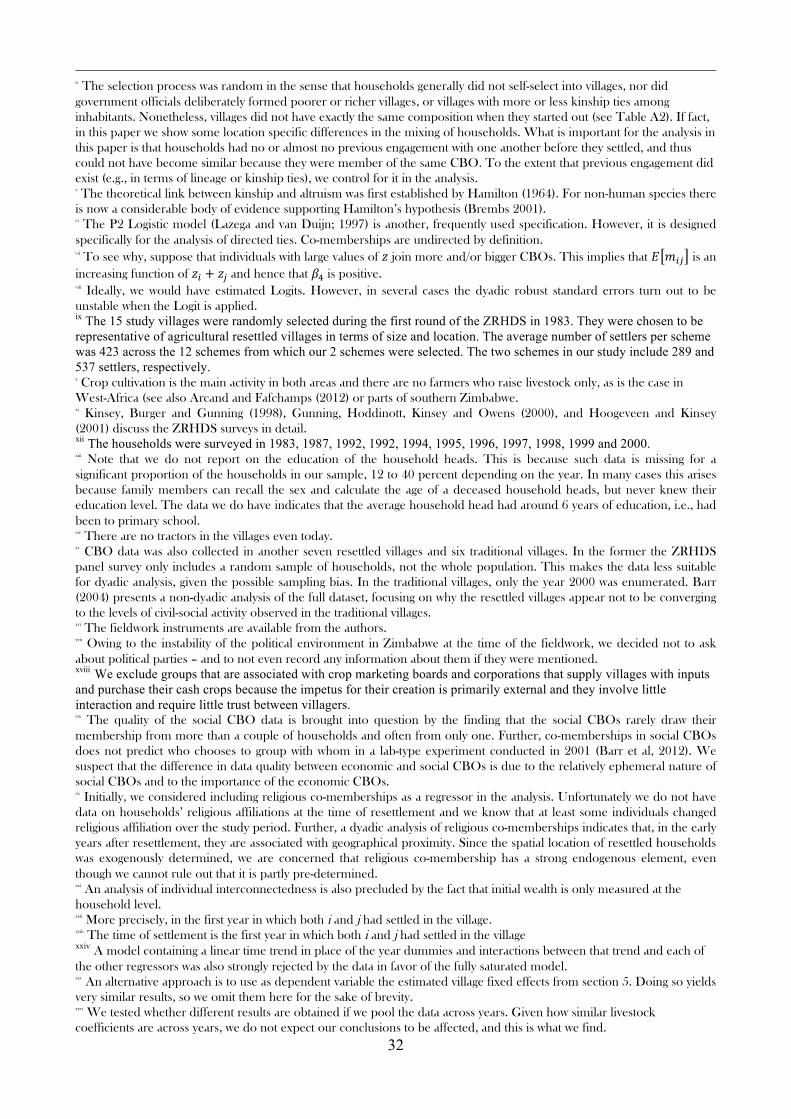
interconnectedness. There is considerable variation across villages, however. Figure 1 plots, for each

village separately, the evolution of the proportion of household dyads sharing at least one co-

membership over time. We see that seven villages had a fully connected network of CBO co-

membership by 1984, while five others had not even reached a density of 20 percent and one village

had no CBO activity until 1991. We also note that the ranking of villages in terms of CBO co-

18

memberships remains fairly stable over time. Figure 2 does the same thing for the average number of

CBO co-memberships. This figure tells a similar story, with each village assuming a very similar rank

to Figure 1.

[Figure 1 and 2 approximately here]

We wish to identify household characteristics at the time of resettlement that predict CBO

formation both within villages and across villages. To study assorting into CBOs within villages, we

need the process of discretionary allocation of settlers to villages (by government officials) to result in

differences in household characteristics within villages. To identify predictors of differences in CBO

membership across villages this process must also have produced sizeable differences in the means of

household characteristics across villages.


The extent of within-village variation is presented in Table 4, which reports summary statistics

for household dyads. Since dyads are only computed within villages, each of these statistics represents

the average difference in a household characteristic across pairs of households residing in the same

village. There are large differences between households in all the characteristics of interest. We also

present the average genetic relatedness, the percentage of dyads having a shared lineage, and the

mean geographical distance between homesteads. As anticipated, mean genetic relatedness is very

low. Under our broad definition, 32 percent of the dyads have a shared lineage. Homesteads are a

third of a kilometre apart on average. This distance is short but it is in line with the planned layout of

resettlement villages in which all residential plots are clustered together. This pattern contrasts with

the traditional layout of Zimbabwean villages where homesteads are scattered around the village

territory and interspersed with arable fields.

19

The extent of across-village variation is summarized in Table A2, which reports village means

for the key regressors of interest, as well as p-values of a Chi square test of equality of means across all

15 villages. We note sizeable and statistically significant variations in village means for all variables.

DYADIC REGRESSION RESULTS

We start by examining the evidence regarding assorting within villages. Table 5 presents

estimated coefficients of a linear probability model where the dependent variable takes value 1 if the

two households in a dyad share a least one co-membership in an economic CBO. Differences across

villages are examined below. Dyadic robust standard errors are reported throughout. Because the

focus of these regressions is exclusively on within-village assorting, we include village fixed effects in all

regressions to net out differences in CBO network density across villages.


To save space, in Table 5 we present estimation results for selected years only – namely, the

first two years and the last years of our panel, plus a few equally interspersed years in between. We

include the first two years because it is important to clearly document the pattern of CBO co-

membership at the time of resettlement. Since key information was collected in 1999 and 2000, we

include the last two years to check for possible artefacts due to survey timing. The estimations for

each panel year from 1982 to 2000 can be found in Appendix Table A3. Point estimates and 90

percent confidence intervals for the most interesting coefficients are presented in Figures 3 to 7.

[Figures 3 to 7 approximately here]

Table 6 presents similar regression results, for the same subset of years, using the number of

co-memberships as the dependent variable. The full set of regression results can be found in

20

Appendix Table A4. Year-by-year point estimates and 90 percent confidence intervals for two of the

regressors are presented in Figures 8 and 9.

With respect to livestock holdings at resettlement, Table 5 and Figure 3 show that households

with different livestock wealth at the time of resettlement were as likely as households with similar

livestock wealth to be co-members in CBOs. Table 5 and Figure 4 show that, in 1982, households

with more livestock were more likely to belong to a CBO than their poorer neighbours. However, by

1983 this effect had disappeared and, from then on, the coefficient on the sum of initial livestock

holdings remains close to 0 and statistically non-significant. Further, this effect is not observed in

Table 6, in which the number of co-memberships is the dependent variable. Taken together, these

findings contradict the hypothesis that CBO formation in resettled villages was elitist. The narrative

that seems to best fit the fact is that better off resettled households set up some economic CBOs upon

arrival and that poorer households joined these CBOs shortly thereafter. Why it is richer households

that set up the first village CBOs is not entirely clear, but one possibility is that poorer settlers, having

just survived the war, had to focus on survival and were not in a position to set up anything. Once

established in their new village, however, they were rapidly allowed to join existing CBOs as and when

their circumstances allowed, so that, over time, initial wealth has no predictive power on CBO

membership. We would not have expected to find this pattern if club membership had served,

through segregation and prejudice, to freeze the socio-economic differentiation present at the time of

resettlement.

Table 5 and Figure 5 show that, from 1986 to 1998, households are more likely to belong to

the same CBO if they settled at around the same time. This effect is observed only seven years after

the resettlement programme started, suggesting that it is driven by the few households who resettled

very late. As time passes, the effect remains and is estimated with increasing precision, but it declines

in magnitude and loses its statistical significance in 1999 and 2000. The same story is told in Table 6,

where the number of co-memberships is the dependent variable. Tables 5 and 6 also show that,

around 1987 (the effect is also observed in 1986 and 1988), late settlers were more likely than early

21

settlers to be CBO members. Taken together, these findings suggest that late settlers either responded

to being excluded from pre-existing CBOs by setting up their own but this, almost competitive,

response was short lived; or never wished to belong to early settler CBOs and set up their own CBOs

with initially considerable – but waning – enthusiasm.

Table 5 and Figure 6 show that, in 1982 and 1983, more geographically proximate households

were more likely to share at least one co-membership. This effect, however, vanished over time, a

finding in accordance with Gans (1968) and Michaelson (1976). However, the effect reappears in

1997 and grows stronger between 1997 and 2000. Could this be due to the increased political

polarization that was growing during that period? We cannot tell.

[Table 6 and Figures 8 and 9 approximately here]

One of the most heartening effects identified by our analysis relates to the gender of the

household heads. Table 6 and Figure 8 show that households with heads of different gender on

average share more rather than fewer co-memberships. This effect persists even when, between 1992

and 1997, female-headed households, on average, appear to be less well connected via the CBO

network (see Figure 9). While the corresponding coefficient in Table 5 and Figure 7 is always

positive, it is rarely significant. We do not know why female-headed households were treated

favorably in the study area. One possible conjecture is that the intervention of the government and the

link between the resettlement program and the war (and thus widowhood) created an atmosphere

more welcoming towards female-headed households.

Pooling data across years increases power and can, thereby, improve inference. To this effect,

we re-estimate the model presented year-by-year in Table 5 using all 19 years of data in a single

regression that also includes year dummies to capture the effect of the passage of time. However,

inferences based on this regression are valid only if the coefficients on the regressors are stable across

22

time. To investigate this, we interact each of the year dummies with each of the other regressors in the

model. These interaction terms are jointly highly significant (p<0.001) indicating that pooling is not

appropriate.xxiv We conduct a similar analysis and reach a similar conclusion for the model presented

year-by-year in Table 6. Based on these analyses, we conclude that inference is best conducted using

the year-by-year results reported above.

VILLAGE LEVEL ANALYSIS

Having discussed assorting patterns within villages, we now turn to the large and significant

differences in CBO network density across villages. For both Tables 5 and 6, village fixed effects are

always jointly significant and explain a large proportion of the variation in the dependent variables. In

1983, village fixed effects account for as much as 63 (Table 5) and 60 percent (Table 6) of the

variation in CBO co-membership. The proportion falls to 24 and 32 percent, respectively, in 2000.

Since we only have data for 15 villages observed over a 19 year period, we are modest in our ambition

of identifying statistically significant predictors of inter-village differences in CBO network density.

We focus on two village-level dependent variables: the village average of 𝑑!", and the village

average of 𝑚!". The first is the density of the village CBO network, i.e., the proportion of household

dyads that have at least one CBO membership in common; the second is the average number of

CBO co-memberships between pairs of households.xxv Each dependent variable is defined for each of

the years between 1982 and 2000.

Before proceeding with the analysis, it is useful to go back over the hypotheses that would be

consistent with particular village-level correlation patterns. First, if wealth varies markedly across

villages and wealthier households are more likely to join CBOs, we expect a positive correlation

between the average wealth of a village and CBO co-membership. Alternatively, if poorer households

benefit more from CBOs, we expect a negative relationship. Second, if shared lineage provides an

alternative foundation for collective action, allowing villagers to dispense from forming CBOs, we

23

expect to find a negative correlation between CBO membership and the density of lineage networks

in each village.

We start by calculating bivariate correlation coefficients between our two dependent variables

and the village means of various household characteristics. We consider the large list of possible

correlates, summarized in Table 7. The Table presents the mean and standard deviation of village

averages in livestock holdings at the time of arrival, and in the density of lineage networks. It also

reports the mean and standard deviation of village means for: the age of household heads; the years of

education of the household heads; the household size; the proportion of non-Zimbabwean

households; the proportion of households who resided in a curfew village during the war; the genetic

relatedness in each village; the number of economic CBOs; the number of households; and a dummy

variable indicating whether the village is located in the southerly cluster rather than in the northerly

cluster. The last variable proxies for regional differences in land quality, in the lineage and region of

origin of settlers, and in the implementation of the resettlement policy and related government

programs. The land around the northern villages is better suited for cash-crop cultivation, while the

land around the southern villages is better suited for small cereals and for mixed farming.


We report simple bivariate correlations for 𝑑!" and 𝑚!" in Tables 8 and 9, respectively. From

Table 8 we note that, for all panel years, the proportion of household dyads sharing a CBO co-

membership is negatively correlated with the mean livestock holdings on arrival. The correlation is

highly significant and the remarkable strength of the correlation is also evident in year-by-year scatter

plots – see Figures 10 and 11 for 1982 and 2000, respectively. In the years immediately following

resettlement, CBO co-membership is negatively correlated with the density of the lineage network.

This relationship is highly significant, but its strength declines over time and is no longer significant

from 1996 onwards. We also observe significantly less CBO co-membership in the southerly cluster,

24

but only until 1996. CBO co-membership is also negatively correlated with the average age of

household heads, but only at the beginning and the end of the study period.


[Figures 10 and 11 approximately here]

For the average number of CBO co-memberships Table 9 shows similar but, generally,

weaker correlations. In all years the number CBO co-memberships is negatively correlated with mean

livestock holdings at resettlement, but in later years the correlation is only significant at the ten percent

level. The negative correlation with the density of the lineage network ceases to be significant after

1989, and the negative correlation with the southerly cluster dummy becomes non-significant after

1987. The negative correlation with the mean age of the household heads is absent in the early years

by stronger in the later years.


The negative correlation with the density of the lineage network is consistent with the

hypothesis that, in these villages at least, shared lineage and CBO activity are substitutes for collective

action. This accords with reported responsibility towards clan members and is in line with the earlier

findings of Barr (2004). The negative correlation with mean livestock holdings is consistent with the

hypothesis that poorer villages engage in more CBO activity because it is of greater value to them.

To investigate the robustness of the negative correlation between the CBO co-membership

and mean livestock holdings, we estimate a series of simple OLS regressions that take the proportion

of dyads sharing at least one CBO membership as dependent variable and include as regressors the

mean livestock holdings at resettlement, the mean age of household head, the density of the lineage

network, and the southerly cluster dummy. These regressors are included because they were shown to

be correlated with inter-village variation in CBO density. One regression is run for each year and the

results are reported in Table 10.xxvi The coefficient on average livestock holdings is significant in every

25

regression; the other coefficients are never significant. We take this as strong evidence of a systematic

negative relationship between CBO formation and average village wealth at the time of resettlement.


FURTHER EXPLORATION INTO THE EFFECTS OF WEALTH ON CBO

FORMATION

The dyadic analysis in Table 5 revealed that, in 1982, wealthier households within each village

engaged in more CBO activity, while the poor appeared to be excluded. By 1983 this effect had

disappeared, a finding we interpreted as suggesting that, when they were ready to join, the poor were

free to join without prejudice. In contrast, the village-level analysis in Table 10 reveals that, from 1982

to 2000, poorer villages engaged in more CBO activity, a finding that is consistent with CBOs being of

greater value to the poor.

In a bid to reconcile these two apparently conflicting findings, we divide the dyadic sample

into two sub-samples, one for the eight poorest villages and one for the richest seven, and we re-

estimate the dyadic regressions on the two sub-samples separately (results not reported). This reveals

that poorer villages drive the significant positive coefficient for the sum of livestock holdings. For

these villages, a significant coefficient is observed in 1982 and 1983, indicating it was the relatively well

off households in the poorest villages that were the most active in setting up the CBOs. Maybe they

realized that, as the richest inhabitants in these poor villages, they would be expected to provide

support to others in times of need. Perhaps they saw setting up CBOs as a way of helping their new

neighbours help themselves – also reducing their own future burden in the process.

DISCUSSION AND CONCLUSIONS

Recent years have witnessed a renewed policy interest in community-based development and

CBOs. The extent to which CBOs can contribute to effective and equitable development strongly

26

depends on where they do and do not emerge and on their socio-economic composition. Given the

cross-sectional nature of most work in this field, recent studies have provided descriptive information

on CBO composition. But they have been unable to satisfactorily address issues of causality, i.e.

whether similarity causes people to associate with one another, or whether CBO co-membership

causes people to become more similar – and thus whether community composition affects CBO

formation.

In this paper, we present unique data on the CBO history of newly formed settlements, the

networks of kinship and lineage ties between villagers, and the characteristics of households at the

time of resettlement. We use these data to investigate who groups with whom in economic CBOs,

knowing that emerging CBOs could not have had any effect on the initial characteristics of their

members, given that villagers had limited prior knowledge of one another.

In the Zimbabwean villages we study, we do not find evidence that CBOs are elitist. True, we

do find that households that were wealthier at resettlement were more actively involved in setting up

CBOs, possibly because they had the time and means to do so. But poorer households joined in

when their circumstances allowed, a few years after resettlement.

In the first few years after resettlement, geographical proximity was a determinant of CBO co-

membership. The effect then declined, only to re-emerge in the late 1990s. Although female headed

households are less likely to belong to a CBO for some of the study years, they are not excluded (or

choose not to exclude themselves) from associating with male-headed households. If anything, on

average they are more likely to share memberships with them. People who resettled later tend not to

join existing CBOs and instead appear to set up new CBOs with other late settlers. Whether this

pattern arises because they are excluded or exclude themselves is unclear.

In the dyadic regressions we find significantly strong correlation between the village of

residence and the likelihood of CBO co-membership, indicating that villages differ considerably in

terms of CBO creation. In a village level analysis, we find that average CBO co-membership is

negatively related to the mean livestock holdings on arrival and that this effect persists throughout the

27

two decades for which we have data. This indicates that villages comprising more poor settlers are

more active in creating CBOs.

With the exception of a positive effect of geographical proximity, we fail to replicate any of

Arcand and Fafchamps’ (2012) findings. We find no effect of shared lineage on who groups with

whom, and only weak evidence that the density of the lineage network affects CBO formation at the

village level. Studying lineage effects is as close as we can get to a concept of ethnicity within our data.

This is because the very large majority of the households in our sample are Shona.

The greatest strength of our analysis is that it is based on data derived from a quasi-

experiment. This being the case, we can safely assume that the measured characteristics of the

households and villages at resettlement determine the structure of the CBOs and not the opposite.

This causal clarity comes at a cost, however. By necessity, the study focuses on a special type of

village, those created by government officials selecting applicant households and assigning them to a

specific location. This raises the question of external validity, i.e., the extent to which are our findings

apply beyond the bounds of Zimbabwe’s resettlement program. We believe that they provide useful

insights – or perhaps points of comparison – for many similar schemes elsewhere in the world, such

as the resettlement of internal and international refugees, the resettlement of people displaced by

public works projects (e.g., dams) or natural calamities (e.g., earthquake or tsunami), and the forced

villagization policies pursued in some countries.

What, if anything, do our findings tell us about CBO formation in African villages in general?

Historically, most African villages were formed when people joined small hamlets spearheaded by

one or two households that settled in the wild. In many cases, late comers to these communities share

ties of kinship with the initial pioneers. However, we know that “stranger” households also join such

emergent communities (see, for instance, Dekker 2004 on the formation of non-resettled villages in

Zimbabwe). Hence, some of our findings are likely to be of general interest, especially those relating

to when each household settled in the history of a village.

28

Other findings suggest that CBO activity is not elitist and that even members of female headed

households, a group often excluded from village life in developing countries, are not excluded from

CBO membership with male headed households. This might best be taken as evidence of what is

possible when villages are created rapidly by government officials. In a world where refugee status is

on the increase, so too are settlements of this type. In the case studied here, the resettlement program

followed a victory over a regime inherited from colonialism. By many of those who resettled, the

program would have been perceived as an opportunity to start afresh and as the division of the spoils

of war in accordance with the socialist ideals of the new nation. It is unclear whether resettled refugees

perceive their own predicament in such a positive light. But they could be encouraged to perceive it as

an individual and collective fresh start.

REFERENCES Arcand, Jean-Louis. and Marcel. Fafchamps (2012) “Matching in community-based organizations”

Journal of Development Economics, 98(2), 203 -219.

Barr, Abigail (2004), “Forging Effective New Communities: The evolution of civil society in

Zimbabwean resettled villages” World Development, 32(10), 1753-66,

Barr, Abigail and Mattea Stein (2008), "Status and egalitarianism in traditional communities: An

analysis of funeral attendance in six Zimbabwean villages", CSAE working paper WPS/2008-26.

Bourdillon, M. (1976) “The Shona peoples : an ethnography of the contemporary Shona, with

special reference to their religion”. Harare: Mambo Press.

Brembs, B. (2001), “Hamilton’s Theory”, in Encyclopaedia of Genetics, Academic Press.

Coate, Stephen and Martin Ravallion (1993), “Reciprocity without commitment: characterization and

performance of informal insurance arrangements” Journal of Development Economics, 40, 1-24.

Coleman, James S. (1988), “Social Capital in the Creation of Human Capital” American Journal of

Sociology, 94(Supplement): S95-S120.

29

De Bock, Ombeline (2014) Participation in semi-formal groups and social integration: Evidence from

rural Rwanda. Paper presented at CSAE conference Economic Development in Africa, March 2014.

https://editorialexpress.com/cgi-bin/conference/download.cgi?db_name=CSAE2014&paper_id=730

De Weerdt, Joachim (2004) “Risk-sharing and Endogenous Network Formation” in Dercon S. (ed)

Insurance Against Poverty.

Dekker, Marleen (2004), Risk, Resettlement and Relations: Social Security in Rural Zimbabwe. PhD

Thesis, Vrije Universiteit. Amsterdam: Thela Thesis.

Edwards, M. and David Hulme (1995), Non-Governmental Organizations: Performance and

Accountability. Beyond the Magic Bullet, London: Earthscan.

Krishnan, Pramila and Emanuela Sciubba (2009) “Links and Architecture in Village Networks” The

Economic Journal, 119(537), pp. 917-949.

Fafchamps, Marcel (2006), “Development and Social Capital” Journal of Development Studies,

42(7).

Fafchamps, Marcel and Flore Gubert (2007). “The Formation of Risk Sharing Networks” Journal of

Development Economics, 83(2):326-50.

Fafchamps, Marcel and Simon Quinn (2012), “Networks and Manufacturing Firms in Africa: Results

from a Randomized Experiment”, University of Oxford, Working Paper.

Gans H. (1968), People and plans: essays on urban problems and solutions. NewYork: Basic.

Gunning, Jan-Willem, John Hoddinott,, Bill Kinsey, and Trudy Owens, (2000). “Revisiting Forever

Gained: Income Dynamics in the Resettlement Areas of Zimbabwe, 1983-1997” Journal of

Development Studies, 36(6).

Hamilton, W. (1964). “The Genetical Evolution of Social Behavior” Journal of Theoretical Biology,

7(1), 52.

30

Hoogeveen, J. and Kinsey, B. (2001). “Land Reform, Growth and Equity: A Sequel” Journal of

Southern African Studies, 27(127), 36.

Kinsey, B. (1982) “Forever gained: resettlement and land policy in the context of national

development in Zimbabwe”, Africa, 52 (3) , 92-113.

Kinsey, B., Burger, K. and Gunning, J. W. (1998). “Coping with Drought in Zimbabwe: Survey

Evidence on Responses of Rural Households to Risk” World Development, 25(1), 89-110.

Krackhardt, David (1987), “QAP Partialling as a Test of Spuriousness” Social Networks, 9: 171-86.

E. Lazega and M.A.J. van Duijn (1997) “Formal Structure and Exchanges of Advice in a Law Firm: A

Random Effects Model”. Social Networks, 19, p.375-397.

Lyle, D. (2007), “Estimating and Interpreting Peer and Role Model Effects from Randomly Assigned

Social Groups at West Point”, Review of Economics and Statistics, 89(2): 289-99.

Mansuri, G. and V. Rao (2004) Community-Based and -Driven Development: A Critical Review,

World Bank Research Observer, 19(1), 1-39

Michaelson, W. (1976) Man and His Urban Environment: A Sociological Approach. Reading, MA:

Addison-Wesley.

Ostrom, Elinor (1990), Governing the Commons: The Evolution of Institutions for Collective Action,

Cambridge University Press, Cambridge.

Palmer, R. (1990) “Land Reform in Zimbabwe 1980-1990.”African Affairs, 89, 163-181.

Platteau, Jean-Philippe and F. Gaspart (2003), “The Risk of Resource Misappropriation in

Community-Driven Development” World Development, 31(10): 1687-1703.

Posner, Richard A. (1980), “A Theory of Primitive Society, with Special Reference to Law” Journal of

Law and Economics, XXIII: 1-53.

Putnam, Robert D. (2000), Bowling Alone, Simon and Schuster, New York.

31

Sacerdote, B. (2001), “Peer Effects with Random Assignment: Results from Dartmouth Roommates”,

The Quarterly Journal of Economics, 116(2): 681-704

Shue, K. (2012), “Executive Networks and Firm Policies: Evidence from the Random Assignment of

MBA Peers”, Working Paper

Snijders, Tom (2007), “Statistical methods for social network dynamics” Oxford University,

mimeograph.

Spierenburg, Marja (2003) Strangers, Spirits and Land Reforms. Conflicts About Land in Dande,

Northern Zimbabwe. PhD Thesis, University of Amsterdam

Stead, W, H. (1946). The Clan Organization and Kinship System of Some Shona Tribes. African

Studies, 5(1), 1-20.

Udry, C.R. and Conley, T.G. (2004). “Social networks in Ghana” Economic Growth Center Working

Paper No. 888, Yale University.

World Bank (1998). “The local level institutions study: Program description and prototype

questionnaire” World Bank Local Level Institutions working paper No. 2. Washington, DC: World

Bank, Local Level Institutions Study Group.

i This issue is very clearly illustrated by an example, taken from the work of Snijders (2007): consider social networks among youths and the decision to take up smoking. Are youths forming links with others who then influence them to smoke, or are smokers linking with each other? Put differently, does the link cause smoking or smoking cause the link? ii Resettlement was voluntary and candidate settlers were free to apply to the government to participate to the program. The government stipulated the following criteria for resettlement, by order of priority: (i) refugees and people displaced by the war; (ii) the landless; and (iii) those with insufficient land to maintain themselves and their families (Kinsey, 1982). Additionally, applicants had to be aged between 25-55 years, married or widowed, and not in formal employment. Challenges to this formal selection process by groups of squatters have been reported (Kinsey, 1982), but they do not apply to the villages/schemes in our sample. Settlers in our sample predominantly come from traditional villages or curfew villages, with a minority coming from towns, commercial farms, or outside Zimbabwe (Dekker, 2004) iii Related household could signal their relatedness when applying and thereby increase their chances of being assigned to the same village. Also, our data indicates that latecomers were often related to existing inhabitants, suggesting some self-selection among latecomers (Dekker, 2004).

32

iv The selection process was random in the sense that households generally did not self-select into villages, nor did government officials deliberately formed poorer or richer villages, or villages with more or less kinship ties among inhabitants. Nonetheless, villages did not have exactly the same composition when they started out (see Table A2). If fact, in this paper we show some location specific differences in the mixing of households. What is important for the analysis in this paper is that households had no or almost no previous engagement with one another before they settled, and thus could not have become similar because they were member of the same CBO. To the extent that previous engagement did exist (e.g., in terms of lineage or kinship ties), we control for it in the analysis. v The theoretical link between kinship and altruism was first established by Hamilton (1964). For non-human species there is now a considerable body of evidence supporting Hamilton’s hypothesis (Brembs 2001). vi The P2 Logistic model (Lazega and van Duijn; 1997) is another, frequently used specification. However, it is designed specifically for the analysis of directed ties. Co-memberships are undirected by definition. vii To see why, suppose that individuals with large values of 𝑧 join more and/or bigger CBOs. This implies that 𝐸 𝑚!" is an increasing function of 𝑧! + 𝑧! and hence that 𝛽! is positive. viii Ideally, we would have estimated Logits. However, in several cases the dyadic robust standard errors turn out to be unstable when the Logit is applied. ix The 15 study villages were randomly selected during the first round of the ZRHDS in 1983. They were chosen to be representative of agricultural resettled villages in terms of size and location. The average number of settlers per scheme was 423 across the 12 schemes from which our 2 schemes were selected. The two schemes in our study include 289 and 537 settlers, respectively. x Crop cultivation is the main activity in both areas and there are no farmers who raise livestock only, as is the case in West-Africa (see also Arcand and Fafchamps (2012) or parts of southern Zimbabwe. xi Kinsey, Burger and Gunning (1998), Gunning, Hoddinott, Kinsey and Owens (2000), and Hoogeveen and Kinsey (2001) discuss the ZRHDS surveys in detail. xii The households were surveyed in 1983, 1987, 1992, 1992, 1994, 1995, 1996, 1997, 1998, 1999 and 2000. xiii Note that we do not report on the education of the household heads. This is because such data is missing for a significant proportion of the households in our sample, 12 to 40 percent depending on the year. In many cases this arises because family members can recall the sex and calculate the age of a deceased household heads, but never knew their education level. The data we do have indicates that the average household head had around 6 years of education, i.e., had been to primary school. xiv There are no tractors in the villages even today. xv CBO data was also collected in another seven resettled villages and six traditional villages. In the former the ZRHDS panel survey only includes a random sample of households, not the whole population. This makes the data less suitable for dyadic analysis, given the possible sampling bias. In the traditional villages, only the year 2000 was enumerated. Barr (2004) presents a non-dyadic analysis of the full dataset, focusing on why the resettled villages appear not to be converging to the levels of civil-social activity observed in the traditional villages. xvi The fieldwork instruments are available from the authors. xvii Owing to the instability of the political environment in Zimbabwe at the time of the fieldwork, we decided not to ask about political parties – and to not even record any information about them if they were mentioned. xviii We exclude groups that are associated with crop marketing boards and corporations that supply villages with inputs and purchase their cash crops because the impetus for their creation is primarily external and they involve little interaction and require little trust between villagers. xix The quality of the social CBO data is brought into question by the finding that the social CBOs rarely draw their membership from more than a couple of households and often from only one. Further, co-memberships in social CBOs does not predict who chooses to group with whom in a lab-type experiment conducted in 2001 (Barr et al, 2012). We suspect that the difference in data quality between economic and social CBOs is due to the relatively ephemeral nature of social CBOs and to the importance of the economic CBOs. xx Initially, we considered including religious co-memberships as a regressor in the analysis. Unfortunately we do not have data on households’ religious affiliations at the time of resettlement and we know that at least some individuals changed religious affiliation over the study period. Further, a dyadic analysis of religious co-memberships indicates that, in the early years after resettlement, they are associated with geographical proximity. Since the spatial location of resettled households was exogenously determined, we are concerned that religious co-membership has a strong endogenous element, even though we cannot rule out that it is partly pre-determined. xxi An analysis of individual interconnectedness is also precluded by the fact that initial wealth is only measured at the household level. xxii More precisely, in the first year in which both i and j had settled in the village. xxiii The time of settlement is the first year in which both i and j had settled in the village xxiv A model containing a linear time trend in place of the year dummies and interactions between that trend and each of the other regressors was also strongly rejected by the data in favor of the fully saturated model. xxv An alternative approach is to use as dependent variable the estimated village fixed effects from section 5. Doing so yields very similar results, so we omit them here for the sake of brevity. xxvi We tested whether different results are obtained if we pool the data across years. Given how similar livestock coefficients are across years, we do not expect our conclusions to be affected, and this is what we find.

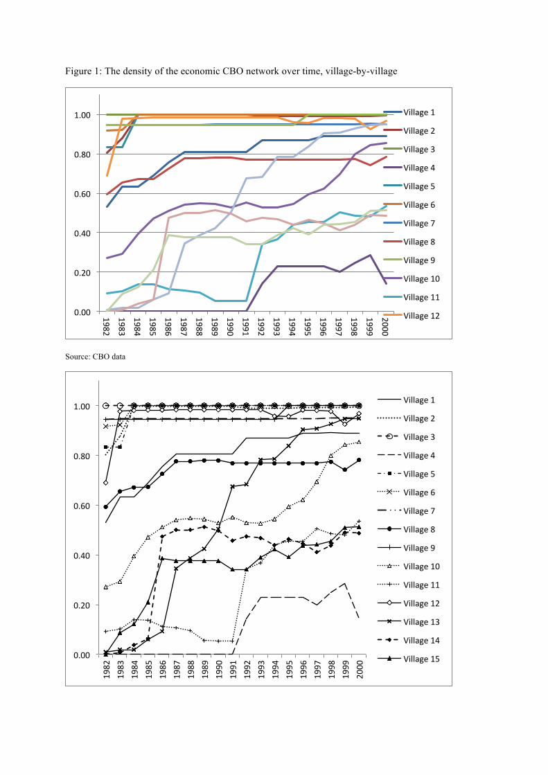
Figure 1: The density of the economic CBO network over time, village-by-village

Source: CBO data

0.00

0.20

0.40

0.60

0.80

1.00

1982

1983

1984

1985

1986

1987

1988

1989

1990

1991

1992

1993

1994

1995

1996

1997

1998

1999

2000

Village 1

Village 2

Village 3

Village 4

Village 5

Village 6

Village 7

Village 8

Village 9

Village 10

Village 11

Village 12

0.00

0.20

0.40

0.60

0.80

1.00

1982

1983

1984

1985

1986

1987

1988

1989

1990

1991

1992

1993

1994

1995

1996

1997

1998

1999

2000

Village 1

Village 2

Village 3

Village 4

Village 5

Village 6

Village 7

Village 8

Village 9

Village 10

Village 11

Village 12

Village 13

Village 14

Village 15

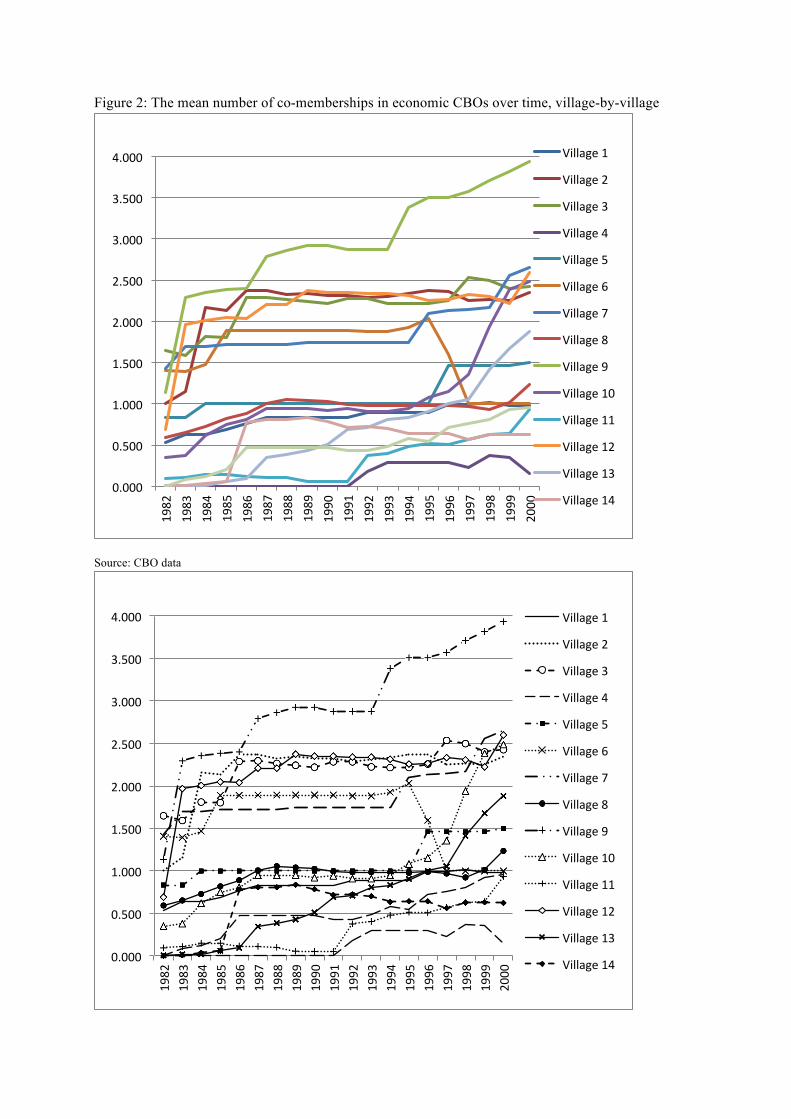
Figure 2: The mean number of co-memberships in economic CBOs over time, village-by-village

Source: CBO data

0.000

0.500

1.000

1.500

2.000

2.500

3.000

3.500

4.000 1982

1983

1984

1985

1986

1987

1988

1989

1990

1991

1992

1993

1994

1995

1996

1997

1998

1999

2000

Village 1

Village 2

Village 3

Village 4

Village 5

Village 6

Village 7

Village 8

Village 9

Village 10

Village 11

Village 12

Village 13

Village 14

0.000

0.500

1.000

1.500

2.000

2.500

3.000

3.500

4.000

1982

1983

1984

1985

1986

1987

1988

1989

1990

1991

1992

1993

1994

1995

1996

1997

1998

1999

2000

Village 1

Village 2

Village 3

Village 4

Village 5

Village 6

Village 7

Village 8

Village 9

Village 10

Village 11

Village 12

Village 13

Village 14

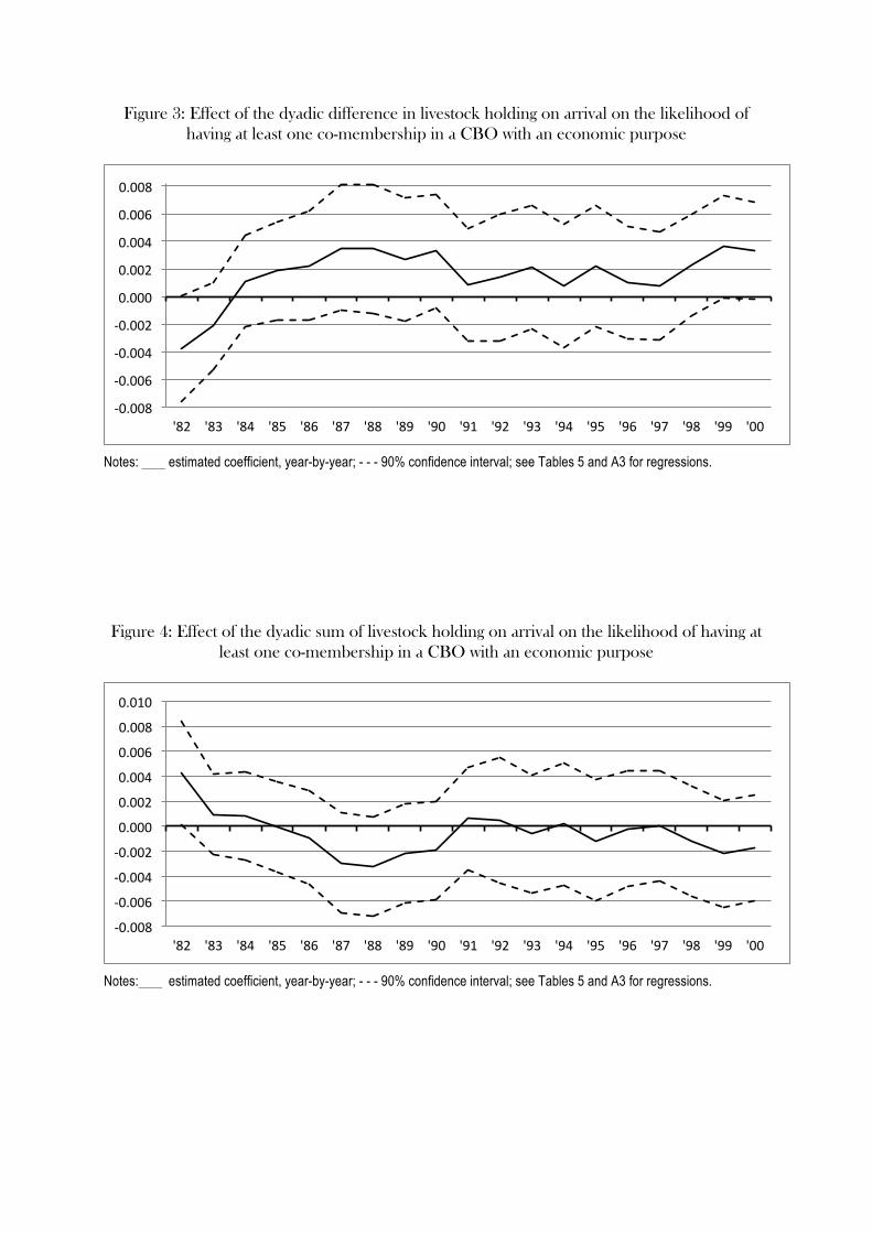
Figure 3: Effect of the dyadic difference in livestock holding on arrival on the likelihood of having at least one co-membership in a CBO with an economic purpose

Notes: estimated coefficient, year-by-year; - - - 90% confidence interval; see Tables 5 and A3 for regressions. Figure 4: Effect of the dyadic sum of livestock holding on arrival on the likelihood of having at

least one co-membership in a CBO with an economic purpose

Notes: estimated coefficient, year-by-year; - - - 90% confidence interval; see Tables 5 and A3 for regressions.

-‐0.008

-‐0.006

-‐0.004

-‐0.002

0.000

0.002

0.004

0.006

0.008

'82 '83 '84 '85 '86 '87 '88 '89 '90 '91 '92 '93 '94 '95 '96 '97 '98 '99 '00

-‐0.008

-‐0.006

-‐0.004

-‐0.002

0.000

0.002

0.004

0.006

0.008

0.010

'82 '83 '84 '85 '86 '87 '88 '89 '90 '91 '92 '93 '94 '95 '96 '97 '98 '99 '00

Figure 5: Effect of the dyadic difference in number of years in village on the likelihood of having at least one co-membership in a CBO with an economic purpose


Figure 6: Effect of the geographic distance between the households in a dyad on the likelihood of them having at least one co-membership in a CBO with an economic purpose


-‐0.070 -‐0.060 -‐0.050 -‐0.040 -‐0.030 -‐0.020 -‐0.010 0.000 0.010 0.020

'82 '83 '84 '85 '86 '87 '88 '89 '90 '91 '92 '93 '94 '95 '96 '97 '98 '99 '00

-‐0.150

-‐0.100

-‐0.050

0.000

0.050

'82 '83 '84 '85 '86 '87 '88 '89 '90 '91 '92 '93 '94 '95 '96 '97 '98 '99 '00

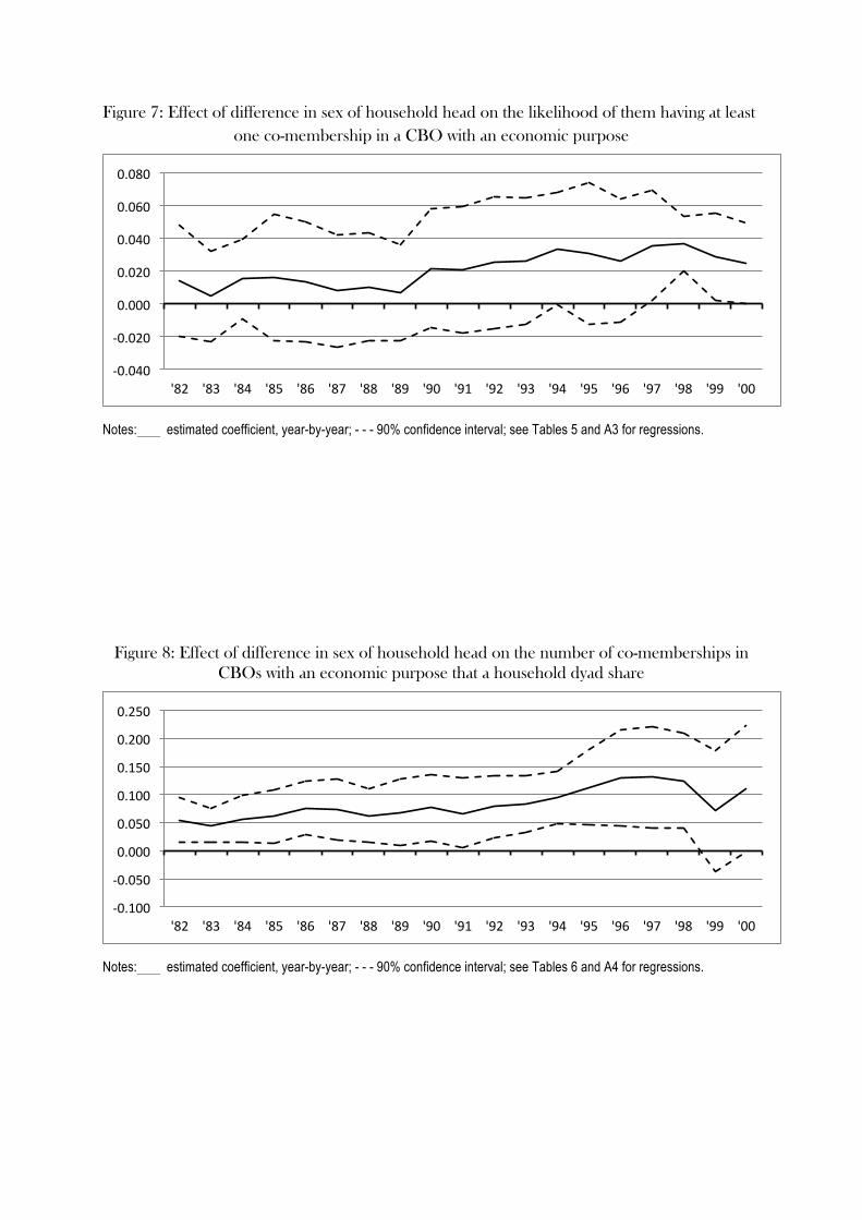
Figure 7: Effect of difference in sex of household head on the likelihood of them having at least one co-membership in a CBO with an economic purpose


Figure 8: Effect of difference in sex of household head on the number of co-memberships in CBOs with an economic purpose that a household dyad share


-‐0.040

-‐0.020

0.000

0.020

0.040

0.060

0.080

'82 '83 '84 '85 '86 '87 '88 '89 '90 '91 '92 '93 '94 '95 '96 '97 '98 '99 '00

-‐0.100

-‐0.050

0.000

0.050

0.100

0.150

0.200

0.250

'82 '83 '84 '85 '86 '87 '88 '89 '90 '91 '92 '93 '94 '95 '96 '97 '98 '99 '00

Figure 9: Effect of both household heads being female on the number of co-memberships in CBOs with an economic purpose that a household dyad shares


-‐0.400

-‐0.300

-‐0.200

-‐0.100

0.000

0.100

0.200

0.300

'82 '83 '84 '85 '86 '87 '88 '89 '90 '91 '92 '93 '94 '95 '96 '97 '98 '99 '00

Figure 10: Village-level relationship between mean livestock wealth on arrival and the density of the economic CBO network (dichotomized) in 1982.

Source: combined data

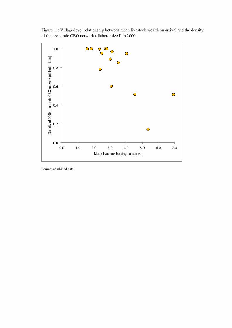
Figure 11: Village-level relationship between mean livestock wealth on arrival and the density of the economic CBO network (dichotomized) in 2000.


0.0

0.2

0.4

0.6

0.8

1.0

0.0 1.0 2.0 3.0 4.0 5.0 6.0 7.0

Dens

ity of

2000

econ

omic

CBO

netw

ork (

dicho

tomize

d)

Mean livestock holdings on arrival

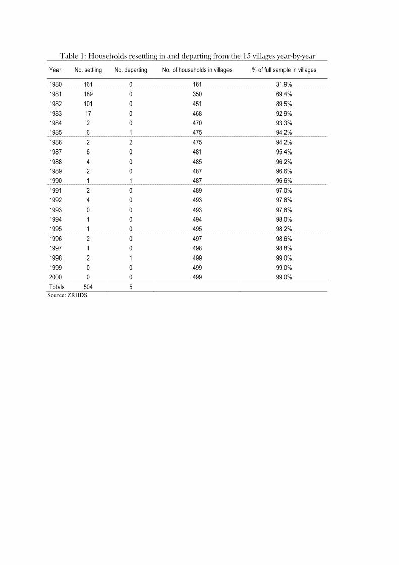
Table 1: Households resettling in and departing from the 15 villages year-by-year

Year No. settling No. departing No. of households in villages % of full sample in villages

1980 161 0 161 31,9%

1981 189 0 350 69,4%

1982 101 0 451 89,5%

1983 17 0 468 92,9%

1984 2 0 470 93,3%

1985 6 1 475 94,2%

1986 2 2 475 94,2%

1987 6 0 481 95,4%

1988 4 0 485 96,2%

1989 2 0 487 96,6%

1990 1 1 487 96,6%

1991 2 0 489 97,0%

1992 4 0 493 97,8%

1993 0 0 493 97,8%

1994 1 0 494 98,0%

1995 1 0 495 98,2%

1996 2 0 497 98,6%

1997 1 0 498 98,8%

1998 2 1 499 99,0%

1999 0 0 499 99,0%

2000 0 0 499 99,0%

Totals 504 5 Source: ZRHDS

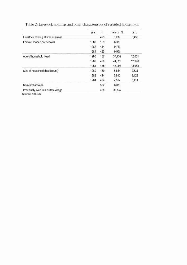
Table 2: Livestock holdings and other characteristics of resettled households

year n mean or % s.d.

Livestock holding at time of arrival

493 3,239 5,438

Female headed households 1980 159 6,3%

1982 444 9,7%

1984 463 9,9%

Age of household head 1980 157 37,732 12,051

1982 436 41,823 12,998

1984 455 43,998 13,053

Size of household (headcount) 1980 159 5,654 2,531

1982 444 6,840 3,128

1984 464 7,517 3,414

Non-Zimbabwean

502 6,8% Previously lived in a curfew village 468 36,5%

Source: ZRHDS

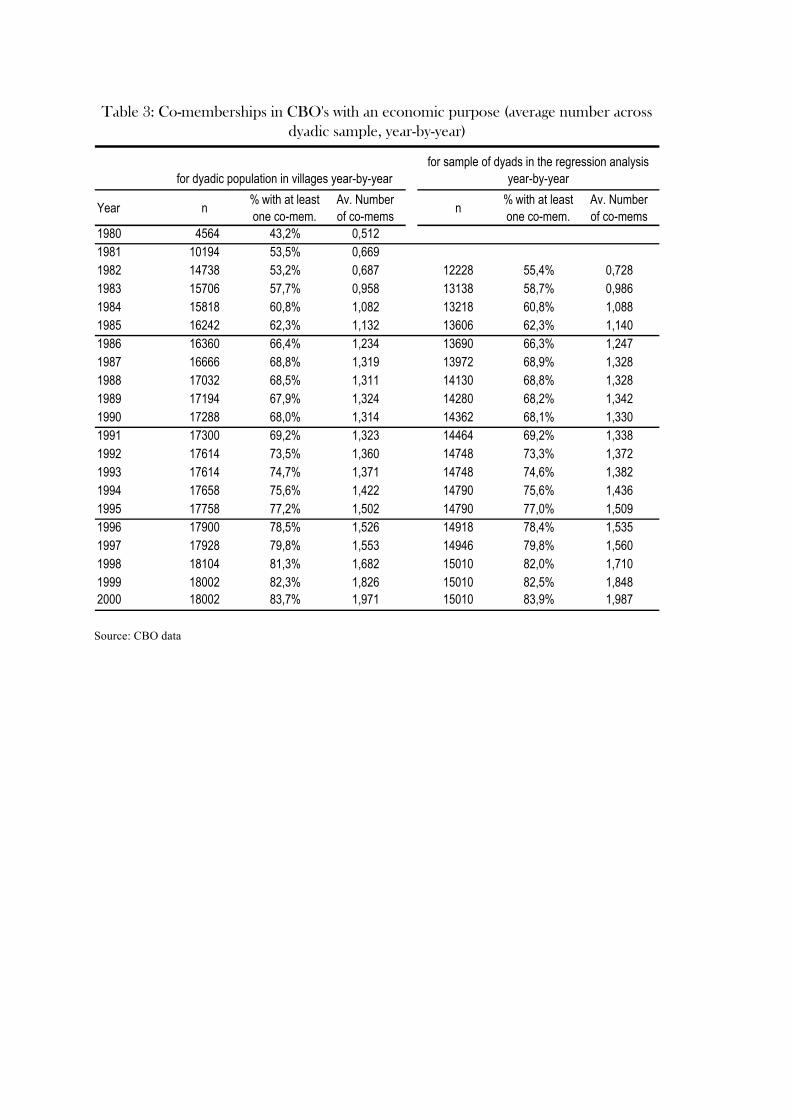
Source: CBO data

Year n % with at least one co-mem.

Av. Number of co-mems n % with at least

one co-mem.Av. Number of co-mems

1980 4564 43,2% 0,5121981 10194 53,5% 0,6691982 14738 53,2% 0,687 12228 55,4% 0,7281983 15706 57,7% 0,958 13138 58,7% 0,9861984 15818 60,8% 1,082 13218 60,8% 1,0881985 16242 62,3% 1,132 13606 62,3% 1,1401986 16360 66,4% 1,234 13690 66,3% 1,2471987 16666 68,8% 1,319 13972 68,9% 1,3281988 17032 68,5% 1,311 14130 68,8% 1,3281989 17194 67,9% 1,324 14280 68,2% 1,3421990 17288 68,0% 1,314 14362 68,1% 1,3301991 17300 69,2% 1,323 14464 69,2% 1,3381992 17614 73,5% 1,360 14748 73,3% 1,3721993 17614 74,7% 1,371 14748 74,6% 1,3821994 17658 75,6% 1,422 14790 75,6% 1,4361995 17758 77,2% 1,502 14790 77,0% 1,5091996 17900 78,5% 1,526 14918 78,4% 1,5351997 17928 79,8% 1,553 14946 79,8% 1,5601998 18104 81,3% 1,682 15010 82,0% 1,7101999 18002 82,3% 1,826 15010 82,5% 1,8482000 18002 83,7% 1,971 15010 83,9% 1,987

for dyadic population in villages year-by-yearfor sample of dyads in the regression analysis

year-by-year

Table 3: Co-memberships in CBO's with an economic purpose (average number across dyadic sample, year-by-year)

Variable n Mean or % s.d. Diff. in livestock holding on arrival 17450 3,986 5,588Diff. in age of household head 16818 14,120 11,026Diff. in size of household (head count, dyadic baseline) 17388 3,407 2,863Diff. in arrival time (1980=0) 18258 1,677 3,210One female headed (dyadic baseline) 17388 0,181 0,385One non-Zimbabwean 18160 0,101 0,302One previously lived in a curfew village 15712 0,232 0,422Genetic relatedness (Hamilton's ratio) 18258 0,012 0,066Shared lineage 17764 32,0%Geographical distance (km) 18258 0,336 0,258Sum of livestock holdings on arrival 17450 6,346 6,904Sum of ages of houdehold heads (1982) 16818 81,992 18,705Sum of sizes of households (dyadic baseline) 17388 12,962 4,599Sum of arrival times (1980=0) 18258 2,949 3,776No. female headed (dyadic baseline) 17388 0,207 0,436No. non-Zimbabwean 18160 0,111 0,330No. previously lived in a curfew village 15712 0,687 0,819Source: combined data

Table 4: Differences and sums of livestock holdings on arrival and other baseline characteristics of household dyads

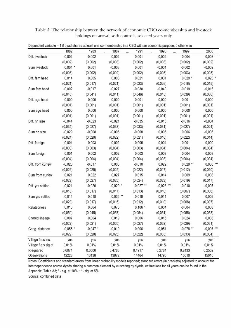
Dependent variable = 1 if dyad shares at least one co-membership in a CBO with an economic purpose, 0 otherwise1982 1983 ... 1987 ... 1991 ... 1995 … 1999 2000

Diff. livestock -0,004 -0,002 0,004 0,001 0,002 0,004 0,003(0,002) (0,002) (0,003) (0,002) (0,003) (0,002) (0,002)

Sum livestock 0,004 * 0,001 -0,003 0,001 -0,001 -0,002 -0,002(0,003) (0,002) (0,002) (0,002) (0,003) (0,003) (0,003)

Diff. fem head 0,014 0,005 0,008 0,021 0,031 0,029 * 0,025 *(0,021) (0,017) (0,021) (0,023) (0,026) (0,016) (0,015)

Sum fem head -0,002 -0,017 -0,027 -0,030 -0,040 -0,019 -0,016(0,040) (0,041) (0,041) (0,046) (0,045) (0,039) (0,036)

Diff. age head 0,000 0,000 0,000 -0,001 0,000 0,001 0,000(0,001) (0,001) (0,001) (0,001) (0,001) (0,001) (0,001)

Sum age head 0,000 0,000 0,000 0,000 0,000 0,000 0,000(0,001) (0,001) (0,001) (0,001) (0,001) (0,001) (0,001)

Diff. hh size -0,044 -0,023 -0,021 -0,035 -0,016 -0,016 -0,004(0,034) (0,027) (0,033) (0,033) (0,031) (0,027) (0,024)

Sum hh size -0,029 -0,008 -0,005 -0,008 0,005 0,006 -0,005(0,024) (0,020) (0,022) (0,021) (0,016) (0,022) (0,014)

Diff. foreign 0,004 0,003 0,002 0,005 0,004 0,001 0,000(0,003) (0,003) (0,004) (0,003) (0,004) (0,004) (0,004)

Sum foreign 0,001 0,002 0,002 0,003 0,003 0,004 0,003(0,004) (0,004) (0,004) (0,004) (0,003) (0,004) (0,004)

Diff. from curfew -0,020 -0,017 0,000 -0,010 0,022 0,029 ** 0,030 ***(0,026) (0,025) (0,025) (0,022) (0,017) (0,012) (0,010)

Sum from curfew 0,021 0,022 0,027 0,015 0,014 0,009 0,008(0,029) (0,027) (0,025) (0,024) (0,023) (0,019) (0,017)

Diff. yrs settled -0,021 -0,020 -0,029 * -0,027 ** -0,028 *** -0,010 -0,007(0,018) (0,017) (0,017) (0,013) (0,010) (0,007) (0,006)

Sum yrs settled 0,014 0,018 0,036 ** 0,018 0,011 0,007 0,002(0,020) (0,017) (0,016) (0,012) (0,010) (0,008) (0,007)

Relatedness 0,016 0,064 0,070 0,106 * 0,004 -0,004 0,008(0,050) (0,045) (0,057) (0,054) (0,051) (0,055) (0,053)

Shared lineage 0,007 0,004 0,019 0,006 0,016 0,024 0,033(0,022) (0,021) (0,026) (0,027) (0,032) (0,029) (0,031)

Geog. distance -0,055 * -0,047 * -0,019 0,006 -0,051 -0,078 ** -0,097 ***(0,029) (0,028) (0,025) (0,022) (0,035) (0,033) (0,034)

Village f.e.s inc. yes yes yes yes yes yes yesVillage f.e.s sig at 0,01% 0,01% 0,01% 0,01% 0,01% 0,01% 0,01%R-squared 0,6074 0,6500 0,4783 0,4917 0,2784 0,2433 0,2562Observations 12228 13138 13972 14464 14790 15010 15010


Table 5: The relationship between the network of economic CBO co-membership and livestock holdings on arrival, with controls, selected years only

Notes: Coefficients and standard errors from linear probability models reported; standard errors (in brackets) adjusted to account for interdependence across dyads sharing a common element by clustering by dyads; estimations for all years can be found in the Appendix, Table A3; * - sig. at 10%; ** - sig. at 5%.

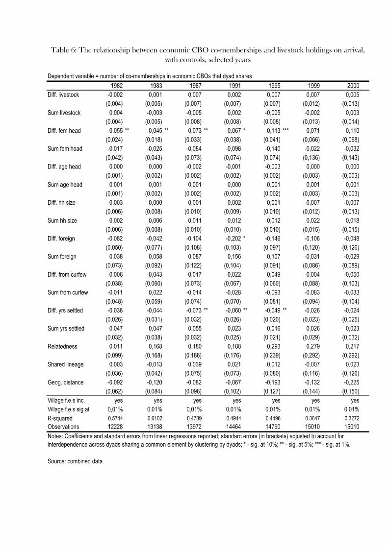
Dependent variable = number of co-memberships in economic CBOs that dyad shares1982 1983 1987 1991 1995 1999 2000

Diff. livestock -0,002 0,001 0,007 0,002 0,007 0,007 0,005(0,004) (0,005) (0,007) (0,007) (0,007) (0,012) (0,013)

Sum livestock 0,004 -0,003 -0,005 0,002 -0,005 -0,002 0,003(0,004) (0,005) (0,008) (0,008) (0,008) (0,013) (0,014)

Diff. fem head 0,055 ** 0,045 ** 0,073 ** 0,067 * 0,113 *** 0,071 0,110(0,024) (0,018) (0,033) (0,038) (0,041) (0,066) (0,068)

Sum fem head -0,017 -0,025 -0,084 -0,098 -0,140 -0,022 -0,032(0,042) (0,043) (0,073) (0,074) (0,074) (0,136) (0,143)

Diff. age head 0,000 0,000 -0,002 -0,001 -0,003 0,000 0,000(0,001) (0,002) (0,002) (0,002) (0,002) (0,003) (0,003)

Sum age head 0,001 0,001 0,001 0,000 0,001 0,001 0,001(0,001) (0,002) (0,002) (0,002) (0,002) (0,003) (0,003)

Diff. hh size 0,003 0,000 0,001 0,002 0,001 -0,007 -0,007(0,006) (0,008) (0,010) (0,009) (0,010) (0,012) (0,013)

Sum hh size 0,002 0,006 0,011 0,012 0,012 0,022 0,018(0,006) (0,008) (0,010) (0,010) (0,010) (0,015) (0,015)

Diff. foreign -0,082 -0,042 -0,104 -0,202 * -0,146 -0,106 -0,048(0,050) (0,077) (0,108) (0,103) (0,097) (0,120) (0,126)

Sum foreign 0,038 0,058 0,087 0,156 0,107 -0,031 -0,029(0,073) (0,092) (0,122) (0,104) (0,091) (0,086) (0,089)

Diff. from curfew -0,006 -0,043 -0,017 -0,022 0,049 -0,004 -0,050(0,038) (0,060) (0,073) (0,067) (0,060) (0,088) (0,103)

Sum from curfew -0,011 0,022 -0,014 -0,028 -0,093 -0,083 -0,033(0,048) (0,059) (0,074) (0,070) (0,081) (0,094) (0,104)

Diff. yrs settled -0,038 -0,044 -0,073 ** -0,060 ** -0,049 ** -0,026 -0,024(0,026) (0,031) (0,032) (0,026) (0,020) (0,023) (0,025)

Sum yrs settled 0,047 0,047 0,055 0,023 0,016 0,026 0,023(0,032) (0,038) (0,032) (0,025) (0,021) (0,029) (0,032)

Relatedness 0,011 0,168 0,180 0,188 0,293 0,279 0,217(0,099) (0,168) (0,186) (0,176) (0,239) (0,292) (0,292)

Shared lineage 0,003 -0,013 0,039 0,021 0,012 -0,007 0,023(0,036) (0,042) (0,075) (0,073) (0,080) (0,116) (0,126)

Geog. distance -0,092 -0,120 -0,082 -0,067 -0,193 -0,132 -0,225(0,062) (0,084) (0,098) (0,102) (0,127) (0,144) (0,150)

Village f.e.s inc. yes yes yes yes yes yes yesVillage f.e.s sig at 0,01% 0,01% 0,01% 0,01% 0,01% 0,01% 0,01%R-squared 0.5744 0.6102 0.4789 0.4944 0.4496 0.3647 0.3272Observations 12228 13138 13972 14464 14790 15010 15010


Table 6: The relationship between economic CBO co-memberships and livestock holdings on arrival, with controls, selected years

Notes: Coefficients and standard errors from linear regressions reported; standard errors (in brackets) adjusted to account for interdependence across dyads sharing a common element by clustering by dyads; * - sig. at 10%; ** - sig. at 5%; *** - sig. at 1%.

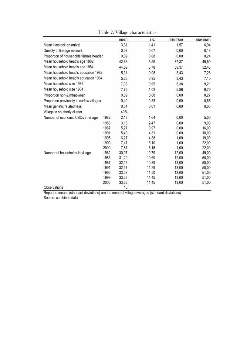
mean s.d. minimum maximumMean livestock on arrival 3,31 1,41 1,57 6,94Density of lineage network 0,07 0,07 0,00 0,18Proportion of households female headed 0,09 0,08 0,00 0,24Mean household head's age 1982 42,33 3,59 37,37 49,59Mean household head's age 1984 44,59 3,78 39,37 52,43Mean household head's education 1982 5,31 0,98 3,43 7,26Mean household head's education 1984 5,23 0,95 3,43 7,10Mean household size 1982 7,03 0,95 5,38 9,21Mean household size 1984 7,72 1,02 5,86 9,79Proportion non-Zimbabwean 0,09 0,08 0,00 0,27Proportion previously in curfew villages 0,40 0,33 0,00 0,85Mean genetic relatedness 0,01 0,01 0,00 0,03Village in southerly cluster 40%Number of economic CBOs in village 1982 2,13 1,64 0,00 5,00

1983 3,13 2,47 0,00 9,001987 5,27 3,97 0,00 16,001991 5,40 4,31 0,00 18,001995 6,27 4,38 1,00 19,001999 7,47 5,10 1,00 22,002000 7,67 5,16 1,00 22,00

Number of households in village 1982 30,07 10,79 12,00 49,001983 31,20 10,60 12,00 50,001987 32,13 10,89 13,00 50,001991 32,67 11,29 13,00 50,001995 33,07 11,50 13,00 51,001999 33,33 11,45 13,00 51,002000 33,33 11,45 13,00 51,00

Observations 15Reported means (standard deviations) are the mean of village averages (standard deviations)Source: combined data

Table 7: Village characteristics

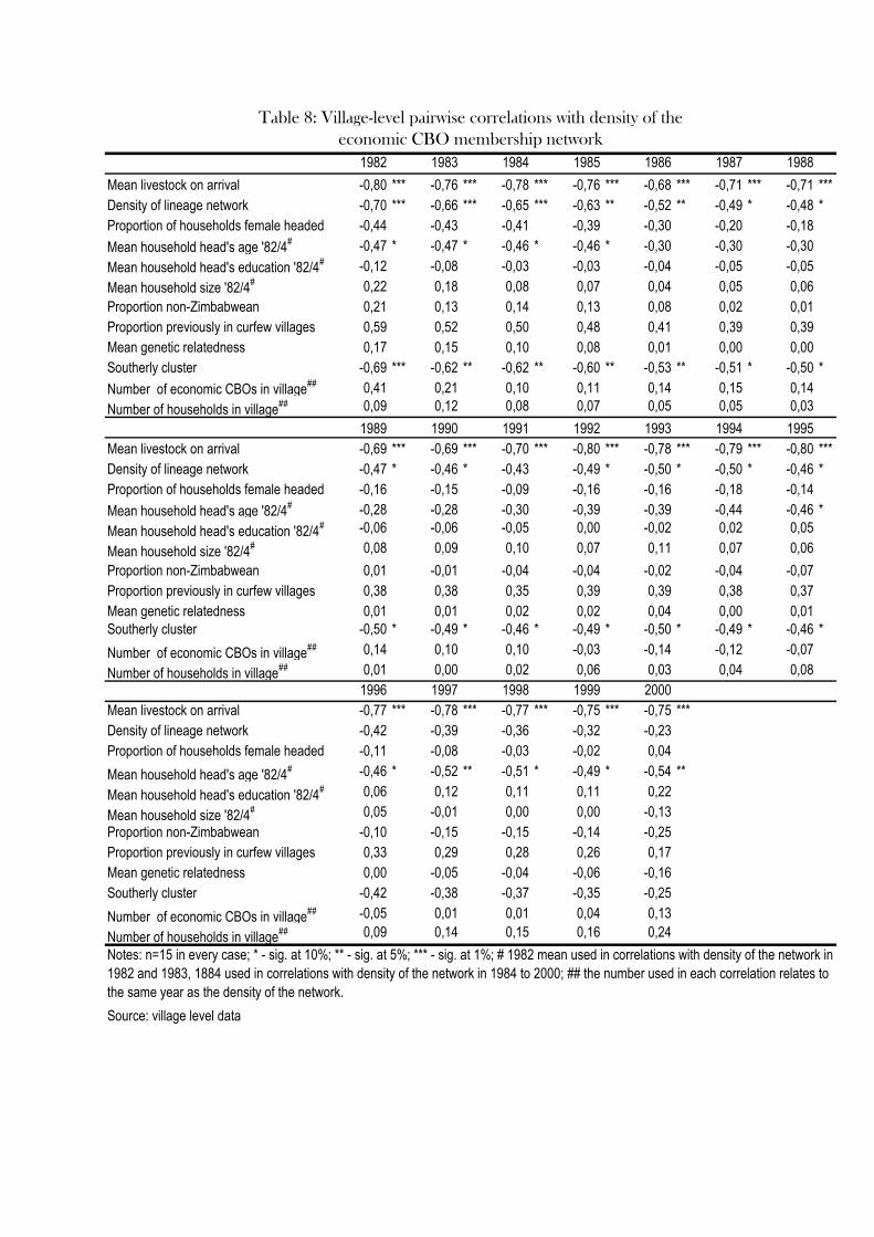
1982 1983 1984 1985 1986 1987 1988Mean livestock on arrival -0,80 *** -0,76 *** -0,78 *** -0,76 *** -0,68 *** -0,71 *** -0,71 ***Density of lineage network -0,70 *** -0,66 *** -0,65 *** -0,63 ** -0,52 ** -0,49 * -0,48 *Proportion of households female headed -0,44 -0,43 -0,41 -0,39 -0,30 -0,20 -0,18Mean household head's age '82/4# -0,47 * -0,47 * -0,46 * -0,46 * -0,30 -0,30 -0,30Mean household head's education '82/4# -0,12 -0,08 -0,03 -0,03 -0,04 -0,05 -0,05Mean household size '82/4# 0,22 0,18 0,08 0,07 0,04 0,05 0,06Proportion non-Zimbabwean 0,21 0,13 0,14 0,13 0,08 0,02 0,01Proportion previously in curfew villages 0,59 0,52 0,50 0,48 0,41 0,39 0,39Mean genetic relatedness 0,17 0,15 0,10 0,08 0,01 0,00 0,00Southerly cluster -0,69 *** -0,62 ** -0,62 ** -0,60 ** -0,53 ** -0,51 * -0,50 *Number of economic CBOs in village## 0,41 0,21 0,10 0,11 0,14 0,15 0,14Number of households in village## 0,09 0,12 0,08 0,07 0,05 0,05 0,03

1989 1990 1991 1992 1993 1994 1995Mean livestock on arrival -0,69 *** -0,69 *** -0,70 *** -0,80 *** -0,78 *** -0,79 *** -0,80 ***Density of lineage network -0,47 * -0,46 * -0,43 -0,49 * -0,50 * -0,50 * -0,46 *Proportion of households female headed -0,16 -0,15 -0,09 -0,16 -0,16 -0,18 -0,14Mean household head's age '82/4# -0,28 -0,28 -0,30 -0,39 -0,39 -0,44 -0,46 *Mean household head's education '82/4# -0,06 -0,06 -0,05 0,00 -0,02 0,02 0,05Mean household size '82/4# 0,08 0,09 0,10 0,07 0,11 0,07 0,06Proportion non-Zimbabwean 0,01 -0,01 -0,04 -0,04 -0,02 -0,04 -0,07Proportion previously in curfew villages 0,38 0,38 0,35 0,39 0,39 0,38 0,37Mean genetic relatedness 0,01 0,01 0,02 0,02 0,04 0,00 0,01Southerly cluster -0,50 * -0,49 * -0,46 * -0,49 * -0,50 * -0,49 * -0,46 *Number of economic CBOs in village## 0,14 0,10 0,10 -0,03 -0,14 -0,12 -0,07Number of households in village## 0,01 0,00 0,02 0,06 0,03 0,04 0,08

1996 1997 1998 1999 2000Mean livestock on arrival -0,77 *** -0,78 *** -0,77 *** -0,75 *** -0,75 ***Density of lineage network -0,42 -0,39 -0,36 -0,32 -0,23Proportion of households female headed -0,11 -0,08 -0,03 -0,02 0,04Mean household head's age '82/4# -0,46 * -0,52 ** -0,51 * -0,49 * -0,54 **Mean household head's education '82/4# 0,06 0,12 0,11 0,11 0,22Mean household size '82/4# 0,05 -0,01 0,00 0,00 -0,13Proportion non-Zimbabwean -0,10 -0,15 -0,15 -0,14 -0,25Proportion previously in curfew villages 0,33 0,29 0,28 0,26 0,17Mean genetic relatedness 0,00 -0,05 -0,04 -0,06 -0,16Southerly cluster -0,42 -0,38 -0,37 -0,35 -0,25Number of economic CBOs in village## -0,05 0,01 0,01 0,04 0,13Number of households in village## 0,09 0,14 0,15 0,16 0,24

Source: village level data

Table 8: Village-level pairwise correlations with density of the economic CBO membership network

Notes: n=15 in every case; * - sig. at 10%; ** - sig. at 5%; *** - sig. at 1%; # 1982 mean used in correlations with density of the network in 1982 and 1983, 1884 used in correlations with density of the network in 1984 to 2000; ## the number used in each correlation relates to the same year as the density of the network.

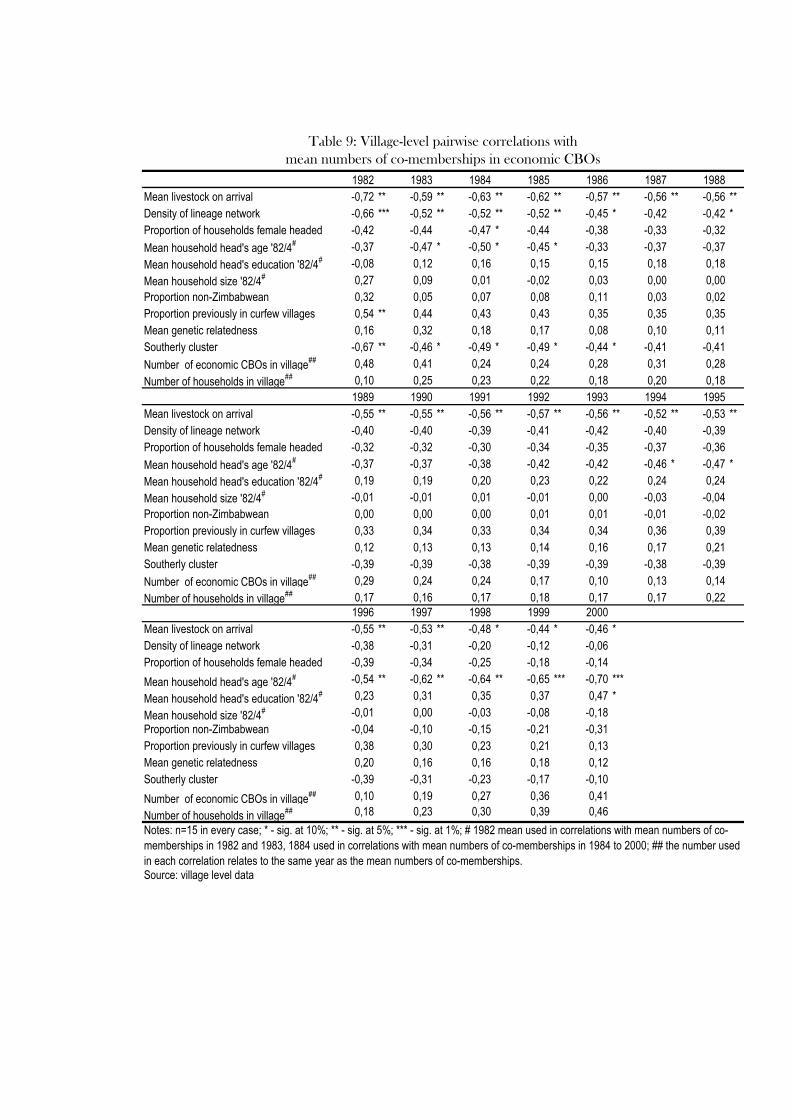
1982 1983 1984 1985 1986 1987 1988Mean livestock on arrival -0,72 ** -0,59 ** -0,63 ** -0,62 ** -0,57 ** -0,56 ** -0,56 **Density of lineage network -0,66 *** -0,52 ** -0,52 ** -0,52 ** -0,45 * -0,42 -0,42 *Proportion of households female headed -0,42 -0,44 -0,47 * -0,44 -0,38 -0,33 -0,32Mean household head's age '82/4# -0,37 -0,47 * -0,50 * -0,45 * -0,33 -0,37 -0,37Mean household head's education '82/4# -0,08 0,12 0,16 0,15 0,15 0,18 0,18Mean household size '82/4# 0,27 0,09 0,01 -0,02 0,03 0,00 0,00Proportion non-Zimbabwean 0,32 0,05 0,07 0,08 0,11 0,03 0,02Proportion previously in curfew villages 0,54 ** 0,44 0,43 0,43 0,35 0,35 0,35Mean genetic relatedness 0,16 0,32 0,18 0,17 0,08 0,10 0,11Southerly cluster -0,67 ** -0,46 * -0,49 * -0,49 * -0,44 * -0,41 -0,41Number of economic CBOs in village## 0,48 0,41 0,24 0,24 0,28 0,31 0,28Number of households in village## 0,10 0,25 0,23 0,22 0,18 0,20 0,18

1989 1990 1991 1992 1993 1994 1995Mean livestock on arrival -0,55 ** -0,55 ** -0,56 ** -0,57 ** -0,56 ** -0,52 ** -0,53 **Density of lineage network -0,40 -0,40 -0,39 -0,41 -0,42 -0,40 -0,39Proportion of households female headed -0,32 -0,32 -0,30 -0,34 -0,35 -0,37 -0,36Mean household head's age '82/4# -0,37 -0,37 -0,38 -0,42 -0,42 -0,46 * -0,47 *Mean household head's education '82/4# 0,19 0,19 0,20 0,23 0,22 0,24 0,24Mean household size '82/4# -0,01 -0,01 0,01 -0,01 0,00 -0,03 -0,04Proportion non-Zimbabwean 0,00 0,00 0,00 0,01 0,01 -0,01 -0,02Proportion previously in curfew villages 0,33 0,34 0,33 0,34 0,34 0,36 0,39Mean genetic relatedness 0,12 0,13 0,13 0,14 0,16 0,17 0,21Southerly cluster -0,39 -0,39 -0,38 -0,39 -0,39 -0,38 -0,39Number of economic CBOs in village## 0,29 0,24 0,24 0,17 0,10 0,13 0,14Number of households in village## 0,17 0,16 0,17 0,18 0,17 0,17 0,22

1996 1997 1998 1999 2000Mean livestock on arrival -0,55 ** -0,53 ** -0,48 * -0,44 * -0,46 *Density of lineage network -0,38 -0,31 -0,20 -0,12 -0,06Proportion of households female headed -0,39 -0,34 -0,25 -0,18 -0,14Mean household head's age '82/4# -0,54 ** -0,62 ** -0,64 ** -0,65 *** -0,70 ***Mean household head's education '82/4# 0,23 0,31 0,35 0,37 0,47 *Mean household size '82/4# -0,01 0,00 -0,03 -0,08 -0,18Proportion non-Zimbabwean -0,04 -0,10 -0,15 -0,21 -0,31Proportion previously in curfew villages 0,38 0,30 0,23 0,21 0,13Mean genetic relatedness 0,20 0,16 0,16 0,18 0,12Southerly cluster -0,39 -0,31 -0,23 -0,17 -0,10Number of economic CBOs in village## 0,10 0,19 0,27 0,36 0,41Number of households in village## 0,18 0,23 0,30 0,39 0,46


Table 9: Village-level pairwise correlations with mean numbers of co-memberships in economic CBOs

Notes: n=15 in every case; * - sig. at 10%; ** - sig. at 5%; *** - sig. at 1%; # 1982 mean used in correlations with mean numbers of co-memberships in 1982 and 1983, 1884 used in correlations with mean numbers of co-memberships in 1984 to 2000; ## the number used in each correlation relates to the same year as the mean numbers of co-memberships.

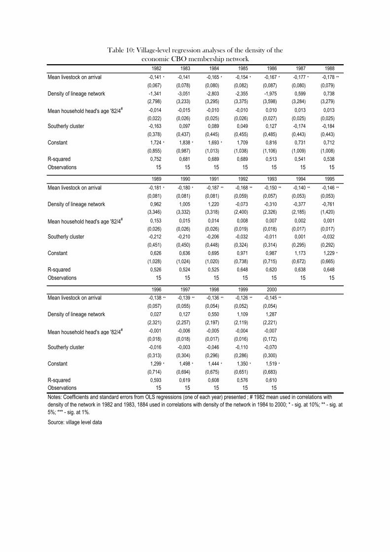
1982 1983 1984 1985 1986 1987 1988Mean livestock on arrival -0,141 * -0,141 -0,165 * -0,154 * -0,167 * -0,177 * -0,178 **

(0,067) (0,078) (0,080) (0,082) (0,087) (0,080) (0,079)Density of lineage network -1,341 -3,051 -2,803 -2,355 -1,975 0,599 0,738

(2,798) (3,233) (3,295) (3,375) (3,598) (3,284) (3,279)

Mean household head's age '82/4# -0,014 -0,015 -0,010 -0,010 0,010 0,013 0,013(0,022) (0,026) (0,025) (0,026) (0,027) (0,025) (0,025)

Southerly cluster -0,163 0,097 0,089 0,049 0,127 -0,174 -0,184(0,378) (0,437) (0,445) (0,455) (0,485) (0,443) (0,443)

Constant 1,724 * 1,838 * 1,693 * 1,709 0,816 0,731 0,712(0,855) (0,987) (1,013) (1,038) (1,106) (1,009) (1,008)

R-squared 0,752 0,681 0,689 0,689 0,513 0,541 0,538Observations 15 15 15 15 15 15 15

1989 1990 1991 1992 1993 1994 1995Mean livestock on arrival -0,181 * -0,180 * -0,187 ** -0,168 ** -0,150 ** -0,140 ** -0,146 **

(0,081) (0,081) (0,081) (0,059) (0,057) (0,053) (0,053)Density of lineage network 0,962 1,005 1,220 -0,073 -0,310 -0,377 -0,761

(3,346) (3,332) (3,318) (2,400) (2,326) (2,185) (1,420)

Mean household head's age '82/4# 0,153 0,015 0,014 0,008 0,007 0,002 0,001(0,026) (0,026) (0,026) (0,019) (0,018) (0,017) (0,017)

Southerly cluster -0,212 -0,210 -0,206 -0,032 -0,011 0,001 -0,032(0,451) (0,450) (0,448) (0,324) (0,314) (0,295) (0,292)

Constant 0,626 0,636 0,695 0,971 0,987 1,173 1,229 *

(1,028) (1,024) (1,020) (0,738) (0,715) (0,672) (0,665)R-squared 0,526 0,524 0,525 0,648 0,620 0,638 0,648Observations 15 15 15 15 15 15 15

1996 1997 1998 1999 2000Mean livestock on arrival -0,138 ** -0,139 ** -0,136 ** -0,126 ** -0,145 **

(0,057) (0,055) (0,054) (0,052) (0,054)Density of lineage network 0,027 0,127 0,550 1,109 1,287

(2,321) (2,257) (2,197) (2,119) (2,221)

Mean household head's age '82/4# -0,001 -0,006 -0,005 -0,004 -0,007(0,018) (0,018) (0,017) (0,016) (0,172)

Southerly cluster -0,016 -0,003 -0,046 -0,110 -0,070(0,313) (0,304) (0,296) (0,286) (0,300)

Constant 1,299 * 1,498 * 1,444 * 1,350 * 1,519 *

(0,714) (0,694) (0,675) (0,651) (0,683)R-squared 0,593 0,619 0,608 0,576 0,610Observations 15 15 15 15 15


Notes: Coefficients and standard errors from OLS regressions (one of each year) presented ; # 1982 mean used in correlations with density of the network in 1982 and 1983, 1884 used in correlations with density of the network in 1984 to 2000; * - sig. at 10%; ** - sig. at 5%; *** - sig. at 1%.

Table 10: Village-level regression analyses of the density of the economic CBO membership network

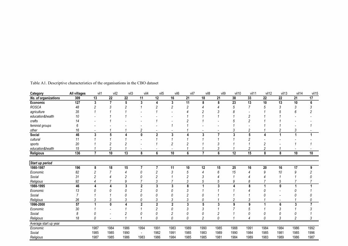
Table A1. Descriptive characteristics of the organisations in the CBO dataset

Category All villages vil1 vil2 vil3 vil4 vil5 vil6 vil7 vil8 vil9 vil10 vil11 vil12 vil13 vil14 vil15No. of organizations 309 13 22 22 11 12 16 21 18 21 38 33 22 22 21 17Economic 127 3 7 5 3 4 3 11 8 8 23 13 10 13 10 6ROSCA 48 2 3 2 1 2 2 2 4 4 5 7 5 3 3 3agriculture 35 1 1 1 - 1 - 4 2 3 8 - 1 5 6 2education&health 10 - 1 1 - - - 1 1 1 1 2 1 1 - -crafts 14 - 1 - - 1 - 2 1 - 5 2 1 1 - -feminist groups 6 - - - - - 1 1 - - 1 - 1 1 - 1other 16 - 1 1 2 - - 1 - - 3 2 1 2 3 -Social 46 3 5 4 0 2 3 4 3 7 3 5 4 1 1 1cultural 11 1 1 1 - 1 1 1 1 1 1 2 - - - -sports 20 1 2 2 - 1 2 2 1 3 1 1 2 - 1 1education&health 15 1 2 1 - - - 1 1 3 1 2 2 1 - -Religious 136 7 10 13 8 6 10 6 7 6 12 15 8 8 10 10

Start up period1980-1987 196 8 18 15 7 7 11 10 12 15 25 16 20 16 17 9Economic 82 2 7 4 0 2 3 5 4 6 15 4 9 10 9 2Social 31 2 4 2 0 2 1 2 3 4 1 4 4 1 1 0Religious 92 4 7 9 7 3 7 3 5 5 9 8 7 5 7 71988-1995 46 4 4 3 2 3 3 8 1 3 4 8 1 0 1 1Economic 13 0 0 0 2 0 0 3 1 1 1 4 0 - 0 1Social 7 1 1 0 0 0 0 2 0 1 1 1 0 - 0 0Religious 26 3 3 3 0 3 3 3 0 1 2 3 1 - 1 01996-2000 57 1 0 4 2 2 2 3 5 3 9 9 1 6 3 7Economic 30 1 - 1 1 2 0 3 3 1 7 5 1 3 1 3Social 8 0 - 2 0 0 2 0 0 2 1 0 0 0 0 1Religious 18 0 - 1 1 0 0 0 2 0 1 4 0 3 2 3Average start up yearEconomic 1987 1984 1986 1994 1991 1983 1989 1990 1985 1988 1991 1984 1984 1986 1992Social 1985 1985 1990 - 1982 1991 1985 1983 1989 1990 1984 1985 1981 1985 1996Religious 1987 1985 1986 1983 1986 1984 1985 1985 1981 1984 1989 1983 1989 1986 1987Source: CBO data

Table A2: Village means of baseline household characteristics

vil1 vil2 vil3 vil4 vil5 vil6 vil7 vil8 vil9 vil10 vil11 vil12 vil13 vil14 vil15

p-value F-test diff in means

Relatedness 0.011 0.004 0.006 0.030 0.010 0.013 0.027 0.007 0.020 0.007 0.003 0.018 0.011 0.011 0.002 0.0001From a curfew village 0.714 0.593 0.357 0.733 0.600 0.600 0.766 0.606 0.848 0.023 0.043 0.000 0.059 0.063 0.000 0.0001Foreign 0.071 0.074 0.214 0.267 0.200 0.200 0.085 0.000 0.060 0.023 0.021 0.000 0.000 0.063 0.090 0.0005Livestock holdings 2.76 2.00 1.84 5.35 1.69 2.70 2.63 2.38 2.74 3.72 3.03 2.99 3.45 4.01 7.25 0.0810Householdsize 7.9 7.8 9.6 9.8 9.5 7.8 7.8 7.3 7.6 7.0 5.9 7.2 8.1 7.6 7.2 0.0001Age head 45.0 41.6 42.9 49.9 43.4 49.5 42.8 43.0 38.9 42.8 40.0 42.6 45.0 53.0 48.3 0.0112Female head 0.142 0.000 0.070 0.000 0.000 0.040 0.020 0.188 0.032 0.211 0.070 0.060 0.193 0.207 0.050 0.0100No. of hh with same lineage in village 6.5 6.6 4.0 5.7 3.1 8.2 18.5 9.9 12.0 10.5 9.0 11.4 9.5 8.8 4.3 0.0100Source of data: combined data set

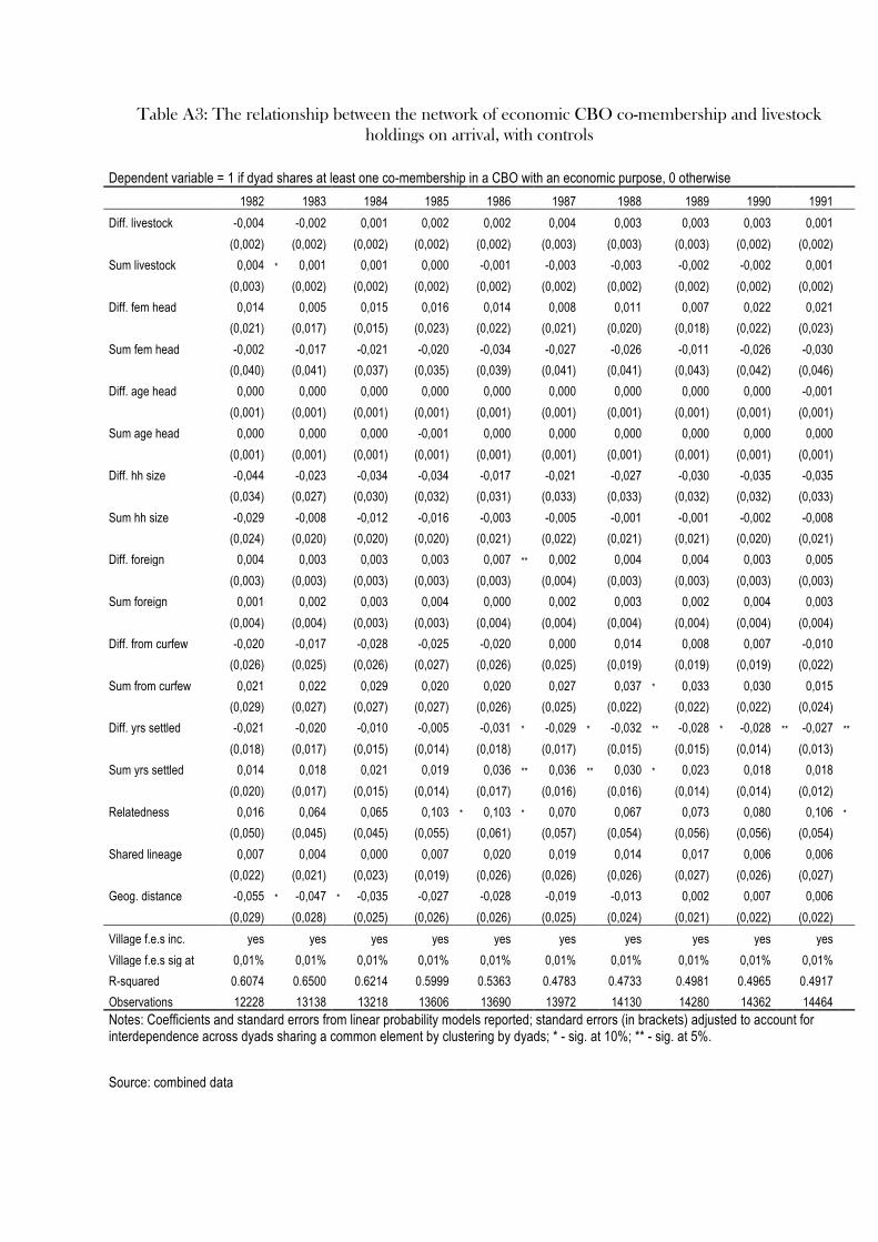
Table A3: The relationship between the network of economic CBO co-membership and livestock holdings on arrival, with controls

Dependent variable = 1 if dyad shares at least one co-membership in a CBO with an economic purpose, 0 otherwise

1982 1983 1984 1985 1986 1987 1988 1989 1990 1991

Diff. livestock -0,004

-0,002

0,001

0,002

0,002

0,004

0,003

0,003

0,003

0,001

(0,002)

(0,002)

(0,002)

(0,002)

(0,002)

(0,003)

(0,003)

(0,003)

(0,002)

(0,002)

Sum livestock 0,004 * 0,001

0,001

0,000

-0,001

-0,003

-0,003

-0,002

-0,002

0,001

(0,003)

(0,002)

(0,002)

(0,002)

(0,002)

(0,002)

(0,002)

(0,002)

(0,002)

(0,002)

Diff. fem head 0,014

0,005

0,015

0,016

0,014

0,008

0,011

0,007

0,022

0,021

(0,021)

(0,017)

(0,015)

(0,023)

(0,022)

(0,021)

(0,020)

(0,018)

(0,022)

(0,023)

Sum fem head -0,002

-0,017

-0,021

-0,020

-0,034

-0,027

-0,026

-0,011

-0,026

-0,030

(0,040)

(0,041)

(0,037)

(0,035)

(0,039)

(0,041)

(0,041)

(0,043)

(0,042)

(0,046)

Diff. age head 0,000

0,000

0,000

0,000

0,000

0,000

0,000

0,000

0,000

-0,001

(0,001)

(0,001)

(0,001)

(0,001)

(0,001)

(0,001)

(0,001)

(0,001)

(0,001)

(0,001)

Sum age head 0,000

0,000

0,000

-0,001

0,000

0,000

0,000

0,000

0,000

0,000

(0,001)

(0,001)

(0,001)

(0,001)

(0,001)

(0,001)

(0,001)

(0,001)

(0,001)

(0,001)

Diff. hh size -0,044

-0,023

-0,034

-0,034

-0,017

-0,021

-0,027

-0,030

-0,035

-0,035

(0,034)

(0,027)

(0,030)

(0,032)

(0,031)

(0,033)

(0,033)

(0,032)

(0,032)

(0,033)

Sum hh size -0,029

-0,008

-0,012

-0,016

-0,003

-0,005

-0,001

-0,001

-0,002

-0,008

(0,024)

(0,020)

(0,020)

(0,020)

(0,021)

(0,022)

(0,021)

(0,021)

(0,020)

(0,021)

Diff. foreign 0,004

0,003

0,003

0,003

0,007 ** 0,002

0,004

0,004

0,003

0,005

(0,003)

(0,003)

(0,003)

(0,003)

(0,003)

(0,004)

(0,003)

(0,003)

(0,003)

(0,003)

Sum foreign 0,001

0,002

0,003

0,004

0,000

0,002

0,003

0,002

0,004

0,003

(0,004)

(0,004)

(0,003)

(0,003)

(0,004)

(0,004)

(0,004)

(0,004)

(0,004)

(0,004)

Diff. from curfew -0,020

-0,017

-0,028

-0,025

-0,020

0,000

0,014

0,008

0,007

-0,010

(0,026)

(0,025)

(0,026)

(0,027)

(0,026)

(0,025)

(0,019)

(0,019)

(0,019)

(0,022)

Sum from curfew 0,021

0,022

0,029

0,020

0,020

0,027

0,037 * 0,033

0,030

0,015

(0,029)

(0,027)

(0,027)

(0,027)

(0,026)

(0,025)

(0,022)

(0,022)

(0,022)

(0,024)

Diff. yrs settled -0,021

-0,020

-0,010

-0,005

-0,031 * -0,029 * -0,032 ** -0,028 * -0,028 ** -0,027 **

(0,018)

(0,017)

(0,015)

(0,014)

(0,018)

(0,017)

(0,015)

(0,015)

(0,014)

(0,013)

Sum yrs settled 0,014

0,018

0,021

0,019

0,036 ** 0,036 ** 0,030 * 0,023

0,018

0,018

(0,020)

(0,017)

(0,015)

(0,014)

(0,017)

(0,016)

(0,016)

(0,014)

(0,014)

(0,012)

Relatedness 0,016

0,064

0,065

0,103 * 0,103 * 0,070

0,067

0,073

0,080

0,106 *

(0,050)

(0,045)

(0,045)

(0,055)

(0,061)

(0,057)

(0,054)

(0,056)

(0,056)

(0,054)

Shared lineage 0,007

0,004

0,000

0,007

0,020

0,019

0,014

0,017

0,006

0,006

(0,022)

(0,021)

(0,023)

(0,019)

(0,026)

(0,026)

(0,026)

(0,027)

(0,026)

(0,027)

Geog. distance -0,055 * -0,047 * -0,035

-0,027

-0,028

-0,019

-0,013

0,002

0,007

0,006

(0,029)

(0,028)

(0,025)

(0,026)

(0,026)

(0,025)

(0,024)

(0,021)

(0,022)

(0,022)

Village f.e.s inc. yes yes yes yes yes yes yes yes yes yes

Village f.e.s sig at 0,01%

0,01%

0,01%

0,01%

0,01%

0,01%

0,01%

0,01%

0,01%

0,01%

R-squared 0.6074

0.6500

0.6214

0.5999

0.5363

0.4783

0.4733

0.4981

0.4965

0.4917

Observations 12228 13138 13218 13606 13690 13972 14130 14280 14362 14464

Notes: Coefficients and standard errors from linear probability models reported; standard errors (in brackets) adjusted to account for interdependence across dyads sharing a common element by clustering by dyads; * - sig. at 10%; ** - sig. at 5%.


Dependent variable = 1 if dyad shares at least one co-membership in a CBO with an economic purpose, 0 otherwise1992 1993 1994 1995 1996 1997 1998 1999 2000

Diff. livestock 0,001 0,002 0,001 0,002 0,001 0,001 0,002 0,004 0,003(0,003) (0,003) (0,003) (0,003) (0,002) (0,002) (0,002) (0,002) (0,002)

Sum livestock 0,000 -0,001 0,000 -0,001 0,000 0,000 -0,001 -0,002 -0,002(0,003) (0,003) (0,003) (0,003) (0,003) (0,003) (0,003) (0,003) (0,003)

Diff. fem head 0,025 0,026 0,034 0,031 0,027 0,036 * 0,037 *** 0,029 * 0,025 *

(0,024) (0,023) (0,021) (0,026) (0,023) (0,020) (0,010) (0,016) (0,015)Sum fem head -0,033 -0,044 -0,054 -0,040 -0,038 -0,041 -0,043 -0,019 -0,016

(0,045) (0,044) (0,043) (0,045) (0,041) (0,041) (0,038) (0,039) (0,036)Diff. age head -0,001 -0,001 0,000 0,000 0,000 0,000 0,000 0,001 0,000

(0,001) (0,001) (0,001) (0,001) (0,001) (0,001) (0,001) (0,001) (0,001)Sum age head 0,000 0,001 0,000 0,000 0,000 0,000 0,000 0,000 0,000

(0,001) (0,001) (0,001) (0,001) (0,001) (0,001) (0,001) (0,001) (0,001)Diff. hh size -0,026 -0,037 -0,038 -0,016 -0,013 -0,005 -0,001 -0,016 -0,004

(0,037) (0,033) (0,038) (0,031) (0,030) (0,025) (0,022) (0,027) (0,024)Sum hh size -0,002 0,006 -0,009 0,005 0,006 0,004 -0,006 0,006 -0,005

(0,021) (0,020) (0,021) (0,016) (0,015) (0,015) (0,015) (0,022) (0,014)Diff. foreign 0,006 * 0,005 0,003 0,004 0,005 0,005 0,004 0,001 0,000

(0,004) (0,004) (0,004) (0,004) (0,003) (0,003) (0,003) (0,004) (0,004)Sum foreign 0,004 0,004 0,005 0,003 0,002 0,002 0,001 0,004 0,003

(0,004) (0,004) (0,004) (0,003) (0,003) (0,003) (0,003) (0,004) (0,004)Diff. from curfew 0,007 0,008 0,007 0,022 0,026 0,026 * 0,016 0,029 ** 0,030 ***

(0,025) (0,024) (0,023) (0,017) (0,016) (0,016) (0,017) (0,012) (0,010)Sum from curfew 0,030 0,026 0,025 0,014 0,015 0,015 0,009 0,009 0,008

(0,025) (0,025) (0,024) (0,023) (0,022) (0,021) (0,022) (0,019) (0,017)Diff. yrs settled -0,031 *** -0,034 *** -0,031 *** -0,028 *** -0,023 ** -0,027 *** -0,017 ** -0,010 -0,007

(0,011) (0,012) (0,010) (0,010) (0,009) (0,009) (0,008) (0,007) (0,006)Sum yrs settled 0,015 0,016 0,009 0,011 0,009 0,014 0,008 0,007 0,002

(0,012) (0,012) (0,011) (0,010) (0,010) (0,010) (0,009) (0,008) (0,007)Relatedness 0,058 0,030 0,005 0,004 -0,005 0,004 0,023 -0,004 0,008

(0,055) (0,052) (0,055) (0,051) (0,053) (0,054) (0,045) (0,055) (0,053)Shared lineage 0,015 0,012 0,018 0,016 0,012 0,026 0,009 0,024 0,033

(0,030) (0,030) (0,030) (0,032) (0,031) (0,029) (0,028) (0,029) (0,031)Geog. distance -0,028 -0,034 -0,045 -0,051 -0,049 -0,070 * -0,077 ** -0,078 ** -0,097 ***

(0,032) (0,032) (0,035) (0,035) (0,034) (0,037) (0,037) (0,033) (0,034)Village f.e.s inc. yes yes yes yes yes yes yes yes yesVillage f.e.s sig at 0,01% 0,01% 0,01% 0,01% 0,01% 0,01% 0,01% 0,01% 0,01%R-squared 0.3281 0.3150 0.2796 0.2784 0.2920 0.2806 0.2681 0.2433 0.2562Observations 14748 14748 14790 14790 14918 14946 15010 15010 15010


Table A3 (cont.): The relationship between the network of economic CBO co-membership and livestock holdings on arrival, with controls

Notes: Coefficients and standard errors from linear probability models reported; standard errors (in brackets) adjusted to account for interdependence across dyads sharing a common element by clustering by dyads; * - sig. at 10%; ** - sig. at 5%; *** - sig. at 1%.

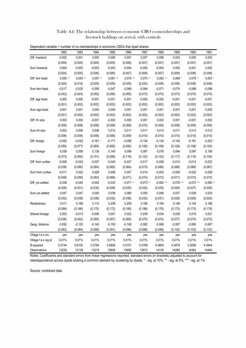
Dependent variable = number of co-memberships in economic CBOs that dyad shares1982 1983 1984 1985 1986 1987 1988 1989 1990 1991

Diff. livestock -0,002 0,001 0,005 0,006 0,007 0,007 0,006 0,003 0,005 0,002(0,004) (0,005) (0,005) (0,005) (0,006) (0,007) (0,007) (0,007) (0,007) (0,007)

Sum livestock 0,004 -0,003 -0,003 -0,003 -0,004 -0,005 -0,004 0,000 -0,001 0,002(0,004) (0,005) (0,006) (0,006) (0,007) (0,008) (0,007) (0,008) (0,008) (0,008)

Diff. fem head 0,055 ** 0,045 ** 0,057 ** 0,061 ** 0,076 *** 0,073 ** 0,062 ** 0,068 * 0,076 ** 0,067 *

(0,024) (0,018) (0,025) (0,029) (0,029) (0,033) (0,029) (0,036) (0,036) (0,038)Sum fem head -0,017 -0,025 -0,056 -0,047 -0,069 -0,084 -0,071 -0,074 -0,088 -0,098

(0,042) (0,043) (0,052) (0,056) (0,065) (0,073) (0,075) (0,073) (0,070) (0,074)Diff. age head 0,000 0,000 -0,001 -0,001 -0,001 -0,002 -0,002 -0,001 -0,001 -0,001

(0,001) (0,002) (0,002) (0,002) (0,002) (0,002) (0,002) (0,002) (0,002) (0,002)Sum age head 0,001 0,001 0,000 0,000 0,001 0,001 0,001 0,001 0,001 0,000

(0,001) (0,002) (0,002) (0,002) (0,002) (0,002) (0,002) (0,002) (0,002) (0,002)Diff. hh size 0,003 0,000 -0,001 -0,003 0,005 0,001 0,002 0,001 -0,001 0,002

(0,006) (0,008) (0,008) (0,008) (0,009) (0,010) (0,009) (0,009) (0,009) (0,009)Sum hh size 0,002 0,006 0,006 0,012 0,011 0,011 0,013 0,011 0,013 0,012

(0,006) (0,008) (0,008) (0,008) (0,009) (0,010) (0,010) (0,010) (0,010) (0,010)Diff. foreign -0,082 -0,042 -0,161 * -0,171 -0,096 -0,104 -0,134 -0,145 -0,161 -0,202 *

(0,050) (0,077) (0,083) (0,085) (0,092) (0,108) (0,109) (0,109) (0,108) (0,103)Sum foreign 0,038 0,058 0,136 0,145 0,099 0,087 0,076 0,094 0,097 0,156

(0,073) (0,092) (0,101) (0,099) (0,119) (0,122) (0,122) (0,117) (0,115) (0,104)Diff. from curfew -0,006 -0,043 -0,057 -0,043 -0,037 -0,017 -0,006 -0,014 -0,014 -0,022

(0,038) (0,060) (0,064) (0,065) (0,064) (0,073) (0,068) (0,068) (0,068) (0,067)Sum from curfew -0,011 0,022 0,028 0,008 0,007 -0,014 -0,002 -0,009 -0,022 -0,028

(0,048) (0,059) (0,063) (0,066) (0,071) (0,074) (0,072) (0,071) (0,070) (0,070)Diff. yrs settled -0,038 -0,044 -0,042 -0,033 -0,071 ** -0,073 ** -0,082 *** -0,078 *** -0,072 *** -0,060 **

(0,026) (0,031) (0,030) (0,028) (0,035) (0,032) (0,029) (0,028) (0,027) (0,026)Sum yrs settled 0,047 0,047 0,045 0,038 0,066 0,055 0,046 0,037 0,028 0,023

(0,032) (0,038) (0,038) (0,032) (0,036) (0,032) (0,031) (0,029) (0,028) (0,025)Relatedness 0,011 0,168 0,115 0,238 0,209 0,180 0,194 0,148 0,144 0,188

(0,099) (0,168) (0,170) (0,172) (0,180) (0,186) (0,176) (0,175) (0,175) (0,176)Shared lineage 0,003 -0,013 -0,006 0,001 0,022 0,039 0,034 0,026 0,019 0,021

(0,036) (0,042) (0,055) (0,057) (0,065) (0,075) (0,074) (0,077) (0,074) (0,073)Geog. distance -0,092 -0,120 -0,140 -0,150 * -0,108 -0,082 -0,068 -0,087 -0,080 -0,067

(0,062) (0,084) (0,089) (0,091) (0,096) (0,098) (0,098) (0,102) (0,102) (0,102)Village f.e.s inc. yes yes yes yes yes yes yes yes yes yesVillage f.e.s sig at 0,01% 0,01% 0,01% 0,01% 0,01% 0,01% 0,01% 0,01% 0,01% 0,01%R-squared 0.5744 0.6102 0.5794 0.5606 0.5151 0.4789 0.4805 0.4979 0.5006 0.4944Observations 12228 13138 13218 13606 13690 13972 14130 14280 14362 14464


Table A4: The relationship between economic CBO co-memberships and livestock holdings on arrival, with controls


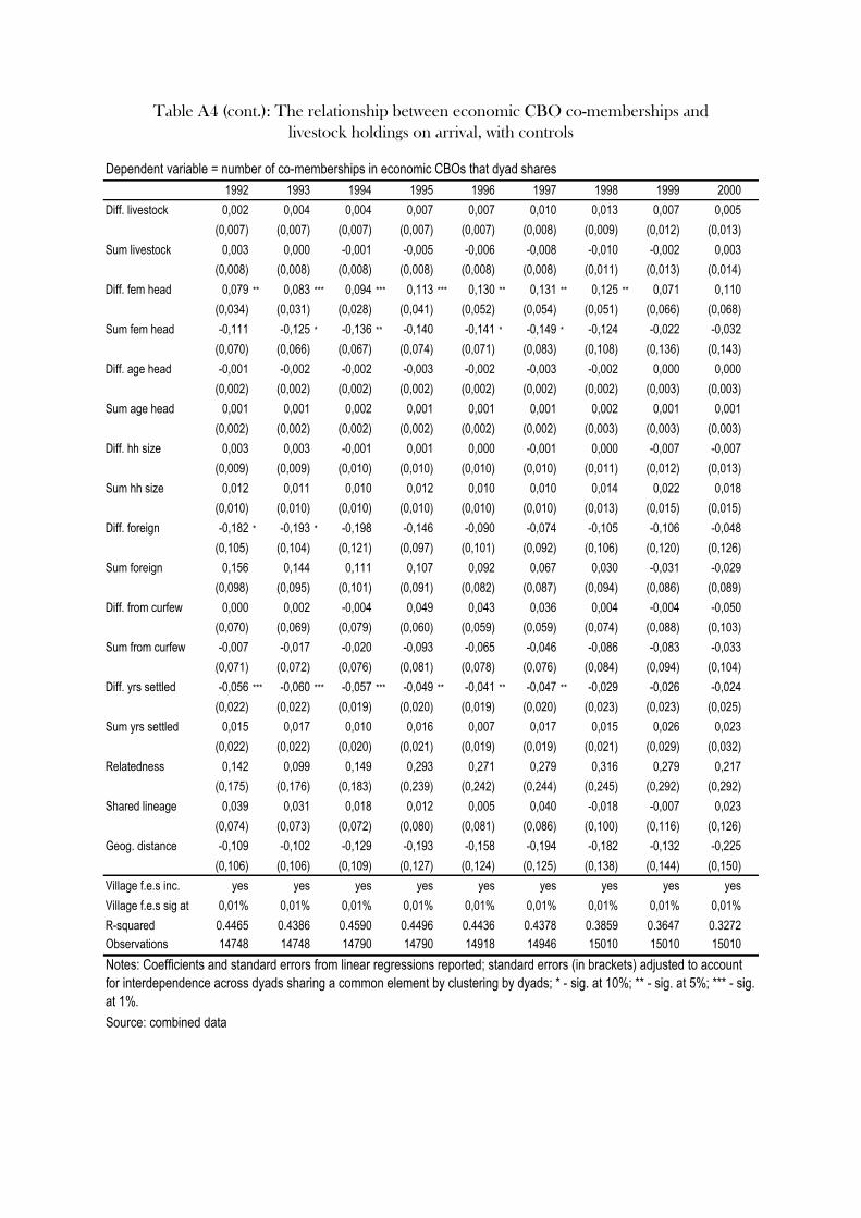
Dependent variable = number of co-memberships in economic CBOs that dyad shares1992 1993 1994 1995 1996 1997 1998 1999 2000

Diff. livestock 0,002 0,004 0,004 0,007 0,007 0,010 0,013 0,007 0,005(0,007) (0,007) (0,007) (0,007) (0,007) (0,008) (0,009) (0,012) (0,013)

Sum livestock 0,003 0,000 -0,001 -0,005 -0,006 -0,008 -0,010 -0,002 0,003(0,008) (0,008) (0,008) (0,008) (0,008) (0,008) (0,011) (0,013) (0,014)

Diff. fem head 0,079 ** 0,083 *** 0,094 *** 0,113 *** 0,130 ** 0,131 ** 0,125 ** 0,071 0,110(0,034) (0,031) (0,028) (0,041) (0,052) (0,054) (0,051) (0,066) (0,068)

Sum fem head -0,111 -0,125 * -0,136 ** -0,140 -0,141 * -0,149 * -0,124 -0,022 -0,032(0,070) (0,066) (0,067) (0,074) (0,071) (0,083) (0,108) (0,136) (0,143)

Diff. age head -0,001 -0,002 -0,002 -0,003 -0,002 -0,003 -0,002 0,000 0,000(0,002) (0,002) (0,002) (0,002) (0,002) (0,002) (0,002) (0,003) (0,003)

Sum age head 0,001 0,001 0,002 0,001 0,001 0,001 0,002 0,001 0,001(0,002) (0,002) (0,002) (0,002) (0,002) (0,002) (0,003) (0,003) (0,003)

Diff. hh size 0,003 0,003 -0,001 0,001 0,000 -0,001 0,000 -0,007 -0,007(0,009) (0,009) (0,010) (0,010) (0,010) (0,010) (0,011) (0,012) (0,013)

Sum hh size 0,012 0,011 0,010 0,012 0,010 0,010 0,014 0,022 0,018(0,010) (0,010) (0,010) (0,010) (0,010) (0,010) (0,013) (0,015) (0,015)

Diff. foreign -0,182 * -0,193 * -0,198 -0,146 -0,090 -0,074 -0,105 -0,106 -0,048(0,105) (0,104) (0,121) (0,097) (0,101) (0,092) (0,106) (0,120) (0,126)

Sum foreign 0,156 0,144 0,111 0,107 0,092 0,067 0,030 -0,031 -0,029(0,098) (0,095) (0,101) (0,091) (0,082) (0,087) (0,094) (0,086) (0,089)

Diff. from curfew 0,000 0,002 -0,004 0,049 0,043 0,036 0,004 -0,004 -0,050(0,070) (0,069) (0,079) (0,060) (0,059) (0,059) (0,074) (0,088) (0,103)

Sum from curfew -0,007 -0,017 -0,020 -0,093 -0,065 -0,046 -0,086 -0,083 -0,033(0,071) (0,072) (0,076) (0,081) (0,078) (0,076) (0,084) (0,094) (0,104)

Diff. yrs settled -0,056 *** -0,060 *** -0,057 *** -0,049 ** -0,041 ** -0,047 ** -0,029 -0,026 -0,024(0,022) (0,022) (0,019) (0,020) (0,019) (0,020) (0,023) (0,023) (0,025)

Sum yrs settled 0,015 0,017 0,010 0,016 0,007 0,017 0,015 0,026 0,023(0,022) (0,022) (0,020) (0,021) (0,019) (0,019) (0,021) (0,029) (0,032)

Relatedness 0,142 0,099 0,149 0,293 0,271 0,279 0,316 0,279 0,217(0,175) (0,176) (0,183) (0,239) (0,242) (0,244) (0,245) (0,292) (0,292)

Shared lineage 0,039 0,031 0,018 0,012 0,005 0,040 -0,018 -0,007 0,023(0,074) (0,073) (0,072) (0,080) (0,081) (0,086) (0,100) (0,116) (0,126)

Geog. distance -0,109 -0,102 -0,129 -0,193 -0,158 -0,194 -0,182 -0,132 -0,225(0,106) (0,106) (0,109) (0,127) (0,124) (0,125) (0,138) (0,144) (0,150)

Village f.e.s inc. yes yes yes yes yes yes yes yes yesVillage f.e.s sig at 0,01% 0,01% 0,01% 0,01% 0,01% 0,01% 0,01% 0,01% 0,01%R-squared 0.4465 0.4386 0.4590 0.4496 0.4436 0.4378 0.3859 0.3647 0.3272Observations 14748 14748 14790 14790 14918 14946 15010 15010 15010


Table A4 (cont.): The relationship between economic CBO co-memberships and livestock holdings on arrival, with controls


An analysis of a quasi-experiment in Zimbabwe INTRODUCTIONfafchamp/BarrDekkerFafchampsCBOs.pdf ·...

Documents

Transcript of An analysis of a quasi-experiment in Zimbabwe INTRODUCTIONfafchamp/BarrDekkerFafchampsCBOs.pdf ·...