An A.M. Radio Project in a Lower-level ECE Class · An AM Radio Project in a Lower -level ECE C...
14
AC 2012-4075: AN A.M. RADIO PROJECT IN A LOWER-LEVEL ECE CLASS Ms. Sheila Patricia Werth, Worcester Polytechnic Institute Sheila Werth is a junior ECE major at Worcester Polytechnic Institute. Her concentration is RF. Mr. Kaung Myat Win, Worcester Polytechnic Institute Dr. Sergey N. Makarov, Worcester Polytechnic Institute Sergey N. Makarov earned his B.S./M.S./Ph.D./D.Sci. degrees at St. Petersburg (Leningrad) State Uni- versity, Russian Federation from the faculty of mathematics and mechanics. Makarov joined the Institute of Mathematics and Mechanics at State St. Petersburg University in 1986 as a researcher and then joined the faculty of State St. Petersburg University, where he became a Full Professor (youngest Full Professor of the faculty) in 1996. In 2000, he joined the faculty of the Department of Electrical and Computer En- gineering at Worcester Polytechnic Institute, Mass., where he became a Full Professor and director of the Center for Electromagnetic Modeling and Design in 2008. His current research interests include WBANs, applied antenna design, and computational electromagnetics. c American Society for Engineering Education, 2012 Page 25.147.1
-
Upload
truongthien -
Category
Documents
-
view
218 -
download
5
Transcript of An A.M. Radio Project in a Lower-level ECE Class · An AM Radio Project in a Lower -level ECE C...
AC 2012-4075: AN A.M. RADIO PROJECT IN A LOWER-LEVEL ECECLASS
Ms. Sheila Patricia Werth, Worcester Polytechnic Institute
Sheila Werth is a junior ECE major at Worcester Polytechnic Institute. Her concentration is RF.
Mr. Kaung Myat Win, Worcester Polytechnic InstituteDr. Sergey N. Makarov, Worcester Polytechnic Institute
Sergey N. Makarov earned his B.S./M.S./Ph.D./D.Sci. degrees at St. Petersburg (Leningrad) State Uni-versity, Russian Federation from the faculty of mathematics and mechanics. Makarov joined the Instituteof Mathematics and Mechanics at State St. Petersburg University in 1986 as a researcher and then joinedthe faculty of State St. Petersburg University, where he became a Full Professor (youngest Full Professorof the faculty) in 1996. In 2000, he joined the faculty of the Department of Electrical and Computer En-gineering at Worcester Polytechnic Institute, Mass., where he became a Full Professor and director of theCenter for Electromagnetic Modeling and Design in 2008. His current research interests include WBANs,applied antenna design, and computational electromagnetics.
c©American Society for Engineering Education, 2012
Page 25.147.1

An AM Radio Project in a Lower-level ECE Class
Abstract
The complex impedance concept has traditionally been a challenge for an introductory ECE
class. An appropriate laboratory exercise may support this concept and spark student interest in
the subject matter. A logical choice is to present a “wireless” project as it naturally includes the
concept of complex impedances.
Building a basic radio receiver on the protoboard is a challenge due to instability of the RF low-
noise amplifier within an unpredictable protoboard environment. Our numerous attempts to build
an AM station receiver on the protoboard have indicated the following difficulties:
1. The circuit can be built by the instructor and by those skilled in the field from the class, but
not by all class students.
2. The design is difficult to debug; sometimes the flawless circuit simply does not function.
3. One critical point is shorting out the power rail of the protoboard (connecting it to the ground
plane of the protoboard). Since this ground plane is made of aluminum and is glued to the
board, such a connection cannot work well for the standard board. We have tried drilling
holes and/or putting clamps; it did not work well in all cases.
4. A laboratory room may be electrically shielded. In our case, the room is located inside the
ECE building and has walls reinforced with a metal grid.
In this paper, we describe an alternative laboratory project that does not make use of the low-
noise amplifier. Instead, we boost the voltage received by a Faraday’s coil using a shunt
capacitor (parallel LCR circuit), purely passively. The RF part of the receiver circuit (coil
antenna, matching capacitor, and an envelope detector with a zero bias Germanium diode) is
purely passive too. Students build a short-range 500-1500kHz complete TX/RX link on every
laboratory bench. A low-cost function generator (Instek), which is a standard bench component,
is used for the transmitter. An external audio modulation is introduced from a computer or iPod.
The laboratory material described was successfully implemented in an introductory ECE class
with mixed major content.
Initial (PCB) Project with AM Radio Receiver
Initially, we set out to build a basic AM radio receiver. This included attempts both with PCB
design and on the protoboard. A photo of the PCB is shown in Figure 1 with the accompanying
schematic shown in Figure 2. This design is composed of four compartmentalized stages to aid in
student understanding. These stages include a resonant LC circuit, a front end amplifier, an
Page 25.147.2
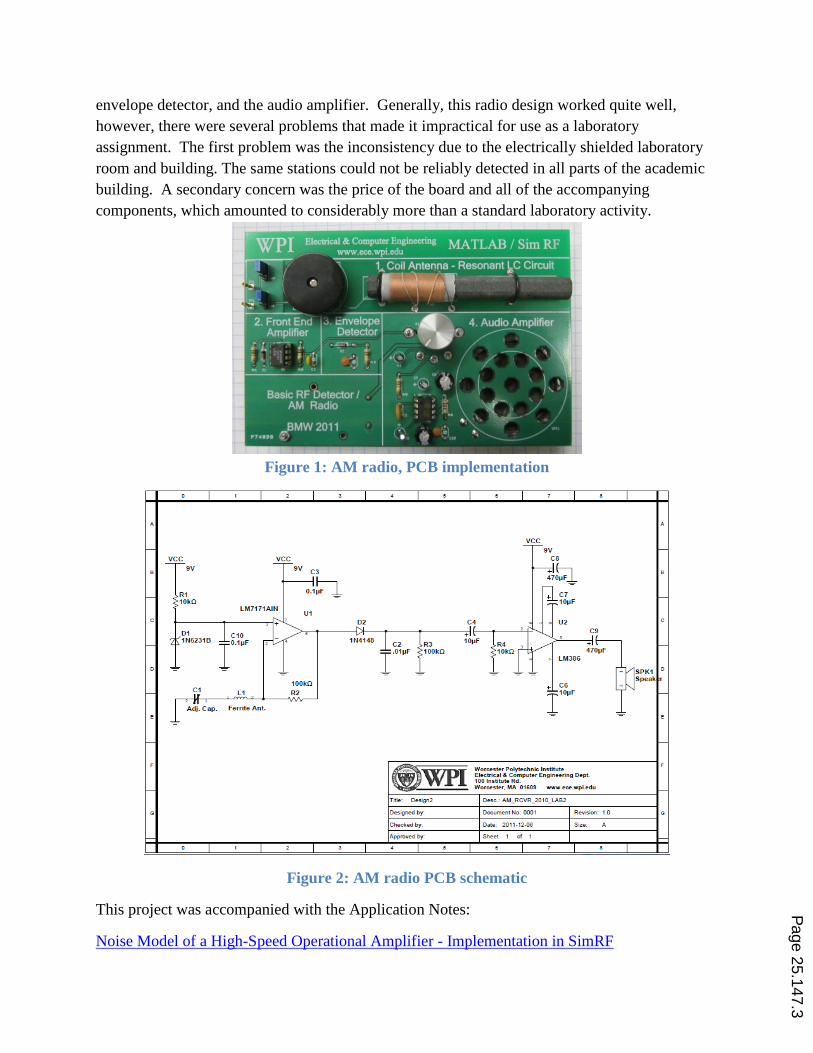
envelope detector, and the audio amplifier. Generally, this radio design worked quite well,
however, there were several problems that made it impractical for use as a laboratory
assignment. The first problem was the inconsistency due to the electrically shielded laboratory
room and building. The same stations could not be reliably detected in all parts of the academic
building. A secondary concern was the price of the board and all of the accompanying
components, which amounted to considerably more than a standard laboratory activity.
Figure 1: AM radio, PCB implementation
Figure 2: AM radio PCB schematic
This project was accompanied with the Application Notes:
Noise Model of a High-Speed Operational Amplifier - Implementation in SimRF
Page 25.147.3
Noise Performance of Inverting and Non-inverting Amplifier Circuits - Implementation in
SimRF
These notes are available at http://ece.wpi.edu/mathworks/. The application notes demonstrate
how to perform a noise analysis of a basic AM receiver using MATLAB’s SimRF. In
conclusion, this was an exciting exercise for a more advanced ECE class, with a strong emphasis
on circuit analysis and design.
Simplified Project with AM Radio Receiver on the Protoboard
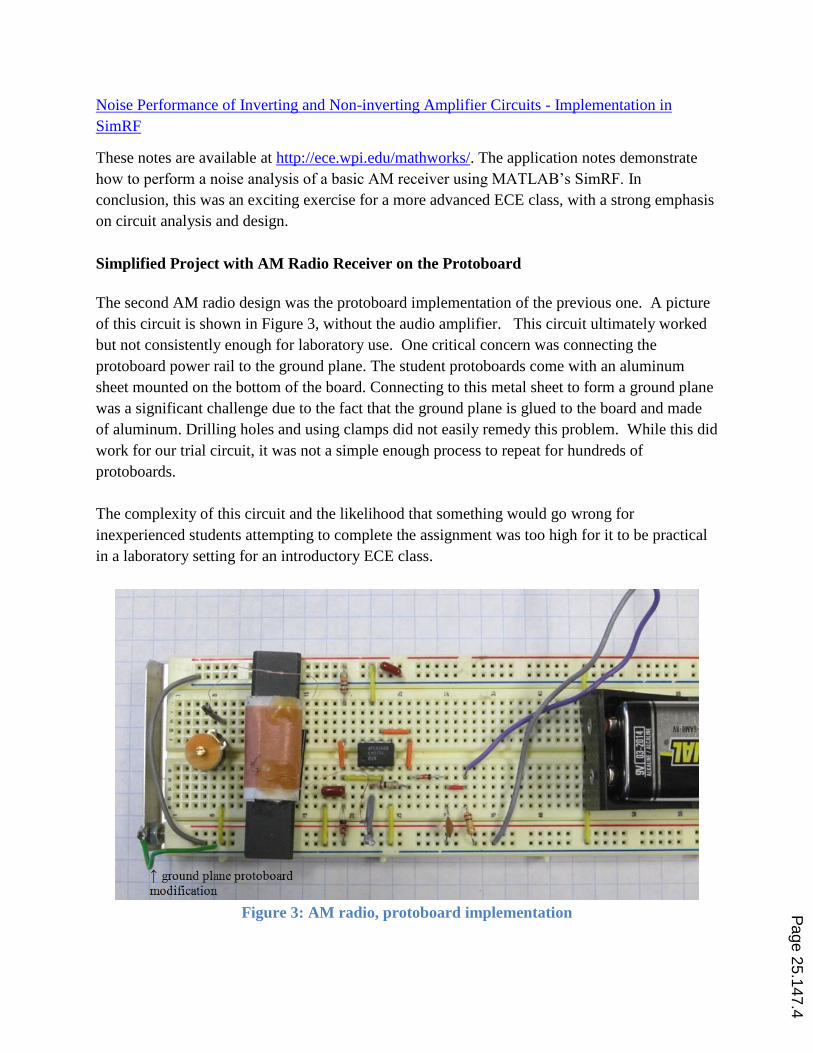
The second AM radio design was the protoboard implementation of the previous one. A picture
of this circuit is shown in Figure 3, without the audio amplifier. This circuit ultimately worked
but not consistently enough for laboratory use. One critical concern was connecting the
protoboard power rail to the ground plane. The student protoboards come with an aluminum
sheet mounted on the bottom of the board. Connecting to this metal sheet to form a ground plane
was a significant challenge due to the fact that the ground plane is glued to the board and made
of aluminum. Drilling holes and using clamps did not easily remedy this problem. While this did
work for our trial circuit, it was not a simple enough process to repeat for hundreds of
protoboards.
The complexity of this circuit and the likelihood that something would go wrong for
inexperienced students attempting to complete the assignment was too high for it to be practical
in a laboratory setting for an introductory ECE class.
Figure 3: AM radio, protoboard implementation P
age 25.147.4
Final Project with on-bench Radio Link
This laboratory project does not rely upon the external AM signal but rather establishes a TX/RX
link on the bench, for every student group. We operate in the near (magnetic) field of two coils.
So, in fact this is a near-field radio link at AM frequencies.
The project was condensed into a handout for students and broken down into four main
subsections. These subsections include:
Part 1. Inductance calculation of an unknown TX coil and setting up the TX circuit
Part 2. Concept of an AM receiver
Part 3. Receiver circuit with envelope detector
Part 4. Complete receiver circuit
These four parts will be presented below as they appeared to students in the laboratory handout
along with a brief description and photographs from the laboratory.
Part 1: Inductance Calculation of an Unknown TX Coil and Setting up the TX Circuit
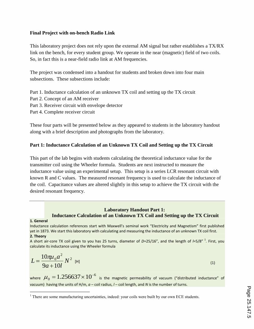
This part of the lab begins with students calculating the theoretical inductance value for the
transmitter coil using the Wheeler formula. Students are next instructed to measure the
inductance value using an experimental setup. This setup is a series LCR resonant circuit with
known R and C values. The measured resonant frequency is used to calculate the inductance of
the coil. Capacitance values are altered slightly in this setup to achieve the TX circuit with the
desired resonant frequency.
Laboratory Handout Part 1:
Inductance Calculation of an Unknown TX Coil and Setting up the TX Circuit 1. General Inductance calculation references start with Maxwell’s seminal work “Electricity and Magnetism” first published yet in 1873. We start this laboratory with calculating and measuring the inductance of an unknown TX coil first. 2. Theory A short air-core TX coil given to you has 25 turns, diameter of D=25/16”, and the length of l=5/8”
1. First, you
calculate its inductance using the Wheeler formula
22
0
109
10N
la
aL
[H] (1)
where 6
0 10256637.1 is the magnetic permeability of vacuum (“distributed inductance” of
vacuum) having the units of H/m, a – coil radius, l – coil length, and N is the number of turns.
1 There are some manufacturing uncertainties, indeed: your coils were built by our own ECE students.
Page 25.147.5
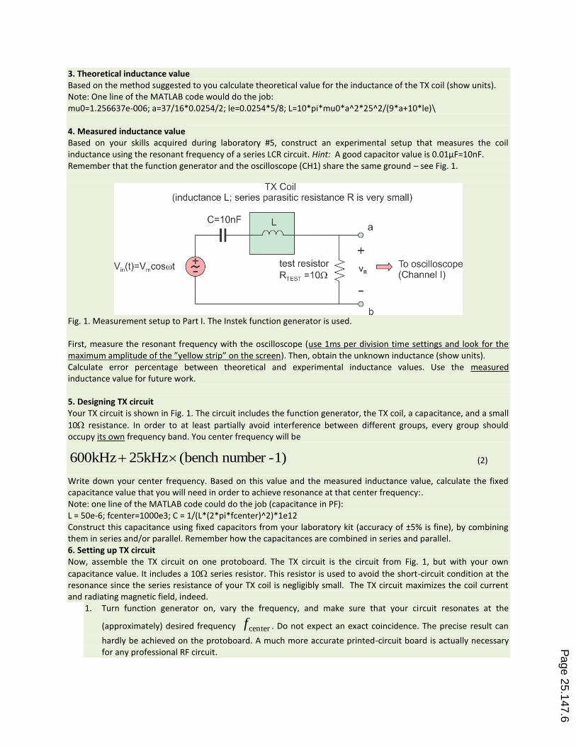
3. Theoretical inductance value Based on the method suggested to you calculate theoretical value for the inductance of the TX coil (show units). Note: One line of the MATLAB code would do the job: mu0=1.256637e-006; a=37/16*0.0254/2; le=0.0254*5/8; L=10*pi*mu0*a^2*25^2/(9*a+10*le)\ 4. Measured inductance value Based on your skills acquired during laboratory #5, construct an experimental setup that measures the coil inductance using the resonant frequency of a series LCR circuit. Hint: A good capacitor value is 0.01µF=10nF. Remember that the function generator and the oscilloscope (CH1) share the same ground – see Fig. 1.
Fig. 1. Measurement setup to Part I. The Instek function generator is used. First, measure the resonant frequency with the oscilloscope (use 1ms per division time settings and look for the maximum amplitude of the ”yellow strip” on the screen). Then, obtain the unknown inductance (show units). Calculate error percentage between theoretical and experimental inductance values. Use the measured inductance value for future work. 5. Designing TX circuit Your TX circuit is shown in Fig. 1. The circuit includes the function generator, the TX coil, a capacitance, and a small
10 resistance. In order to at least partially avoid interference between different groups, every group should occupy its own frequency band. You center frequency will be
1)-numberbench (kHz25kHz600 (2)
Write down your center frequency. Based on this value and the measured inductance value, calculate the fixed capacitance value that you will need in order to achieve resonance at that center frequency:. Note: one line of the MATLAB code could do the job (capacitance in PF): L = 50e-6; fcenter=1000e3; C = 1/(L*(2*pi*fcenter)^2)*1e12 Construct this capacitance using fixed capacitors from your laboratory kit (accuracy of ±5% is fine), by combining them in series and/or parallel. Remember how the capacitances are combined in series and parallel. 6. Setting up TX circuit Now, assemble the TX circuit on one protoboard. The TX circuit is the circuit from Fig. 1, but with your own
capacitance value. It includes a 10 series resistor. This resistor is used to avoid the short-circuit condition at the resonance since the series resistance of your TX coil is negligibly small. The TX circuit maximizes the coil current and radiating magnetic field, indeed.
1. Turn function generator on, vary the frequency, and make sure that your circuit resonates at the
(approximately) desired frequency centerf . Do not expect an exact coincidence. The precise result can
hardly be achieved on the protoboard. A much more accurate printed-circuit board is actually necessary for any professional RF circuit.
Page 25.147.6
2. You might want to add or subtract small capacitance values in order to obtain a better agreement. Do not turn function generator off.
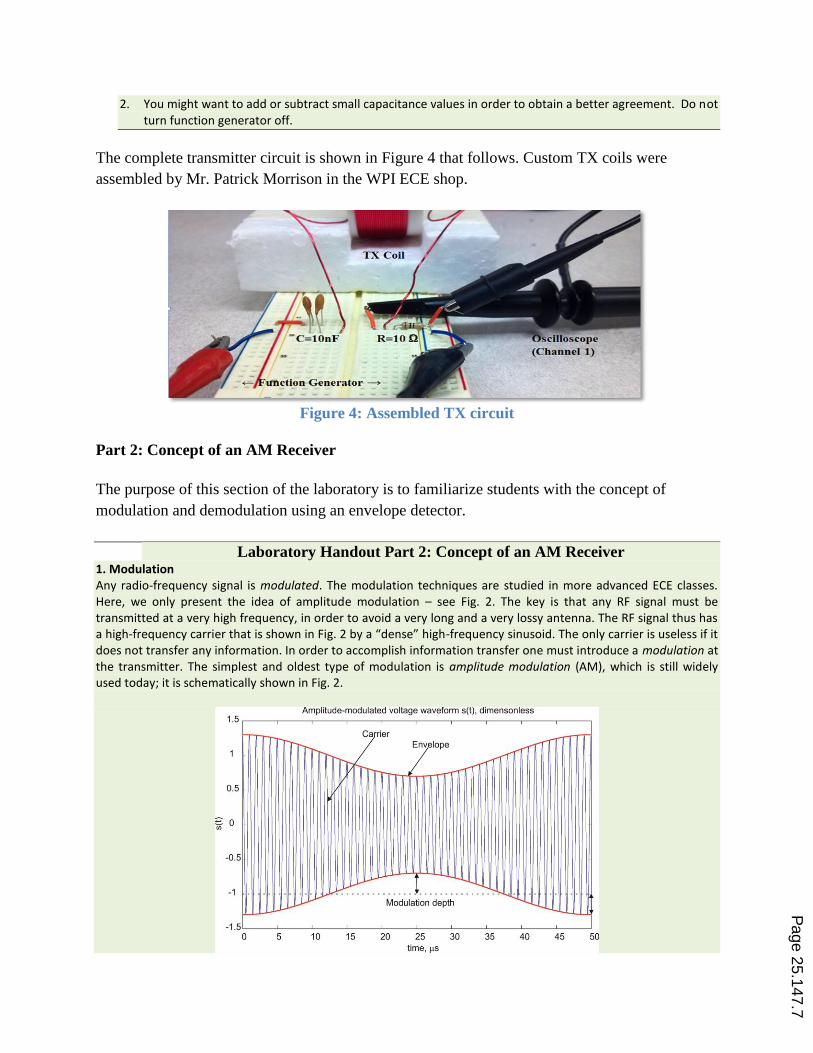
The complete transmitter circuit is shown in Figure 4 that follows. Custom TX coils were
assembled by Mr. Patrick Morrison in the WPI ECE shop.
Figure 4: Assembled TX circuit
Part 2: Concept of an AM Receiver
The purpose of this section of the laboratory is to familiarize students with the concept of
modulation and demodulation using an envelope detector.
Laboratory Handout Part 2: Concept of an AM Receiver 1. Modulation Any radio-frequency signal is modulated. The modulation techniques are studied in more advanced ECE classes. Here, we only present the idea of amplitude modulation – see Fig. 2. The key is that any RF signal must be transmitted at a very high frequency, in order to avoid a very long and a very lossy antenna. The RF signal thus has a high-frequency carrier that is shown in Fig. 2 by a “dense” high-frequency sinusoid. The only carrier is useless if it does not transfer any information. In order to accomplish information transfer one must introduce a modulation at the transmitter. The simplest and oldest type of modulation is amplitude modulation (AM), which is still widely used today; it is schematically shown in Fig. 2.
Page 25.147.7
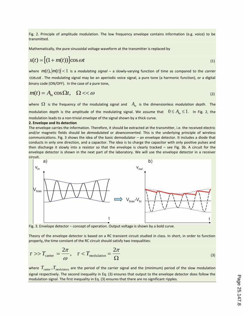
Fig. 2. Principle of amplitude modulation. The low frequency envelope contains information (e.g. voice) to be transmitted. Mathematically, the pure sinusoidal voltage waveform at the transmitter is replaced by
ttmts cos))(1()( (1)
where 1)(),( tmtm is a modulating signal – a slowly-varying function of time as compared to the carrier
tcos . The modulating signal may be an aperiodic voice signal, a pure tone (a harmonic function), or a digital
binary code (ON/OFF). In the case of a pure tone,
,cos)( tAtm m (2)
where is the frequency of the modulating signal and mA is the dimensionless modulation depth. The
modulation depth is the amplitude of the modulating signal. We assume that 10 mA . In Fig. 2, the
modulation leads to a non-trivial envelope of the signal shown by a thick curve. 2. Envelope and its detection The envelope carries the information. Therefore, it should be extracted at the transmitter, i.e. the received electric and/or magnetic fields should be demodulated or downconverted. This is the underlying principle of wireless communications. Fig. 3 shows the idea of the basic demodulator – an envelope detector. It includes a diode that conducts in only one direction, and a capacitor. The idea is to charge the capacitor with only positive pulses and then discharge it slowly into a resistor so that the envelope is clearly tracked – see Fig. 3b. A circuit for the envelope detector is shown in the next part of the laboratory. We will use the envelope detector in a receiver circuit.
Fig. 3. Envelope detector – concept of operation. Output voltage is shown by a bold curve. Theory of the envelope detector is based on a RC transient circuit studied in class. In short, in order to function properly, the time constant of the RC circuit should satisfy two inequalities:
2,
2modulationcarrier TT (3)
where modulationcarrier ,TT are the period of the carrier signal and the (minimum) period of the slow modulation
signal respectively. The second inequality in Eq. (3) ensures that output to the envelope detector does follow the modulation signal. The first inequality in Eq. (3) ensures that there are no significant ripples.
Page 25.147.8

Part 3: Receiver Circuit with Envelope Detector
This section of the laboratory involves the construction of a parallel LC receiver circuit and
accompanying envelope detector. The parallel LC circuit uses a ferrite core coil antenna and a
variable matching capacitor to receive the signal from the transmitter circuit constructed in part
one. Students are instructed to ‘tune’ the receiver circuit by adjusting the matching capacitor and
measure the envelope voltage.
Laboratory Handout Part 3: Receiver Circuit with Envelope Detector 1. Circuit diagram and its understanding The high-frequency part of the circuit is shown in Fig. 4 that follows. It includes two major components:
1. A coil antenna (small magnetic-core coil) and a matching circuit (variable capacitor in parallel). 2. Envelope detector circuit discussed in Part II.
Indeed, the receiver circuit uses the parallel LC circuit (see laboratory #5). This is in contrast to the transmitter with the series LC circuit.
Fig. 4. High-frequency receiver circuit. 2. Circuit assembly 1. Build the receiver circuit shown in Fig. 4. Use another protoboard (about a half of it). This circuit is purely passive; it is not powered by any power supply. It does not have an RF front-end amplifier either. Please, be very careful in handling the coil with the magnetic core. Its leads may be easily broken. 2. Turn on the transmitter and make sure that both coils are in a collinear configuration, at the distance of about 6” apart. The output to the receiver circuit is to be measured with the oscilloscope (DC coupled). Tune the variable capacitor and achieve the maximum output DC voltage (achieve resonance at the receiver). This DC voltage is exactly the envelope of the high-frequency TX wave. Measure the envelope voltage and record its value (show units). In order to change the envelope you must introduce the modulation. The simple (handshaking) modulation is to quickly rotate the amplitude knob of the function generator and see what happens to the DC voltage on the oscilloscope screen.
Page 25.147.9
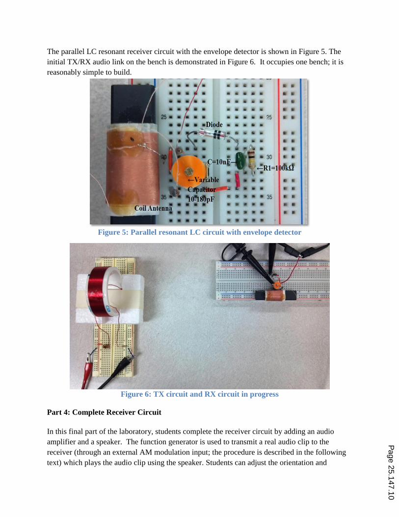
The parallel LC resonant receiver circuit with the envelope detector is shown in Figure 5. The
initial TX/RX audio link on the bench is demonstrated in Figure 6. It occupies one bench; it is
reasonably simple to build.
Figure 5: Parallel resonant LC circuit with envelope detector
Figure 6: TX circuit and RX circuit in progress
Part 4: Complete Receiver Circuit
In this final part of the laboratory, students complete the receiver circuit by adding an audio
amplifier and a speaker. The function generator is used to transmit a real audio clip to the
receiver (through an external AM modulation input; the procedure is described in the following
text) which plays the audio clip using the speaker. Students can adjust the orientation and
Page 25.147.10
location of transmitting and receiving antennas so that they can observe the effects of proximity
and polarization on the received signals amplitude. This exercise is important.
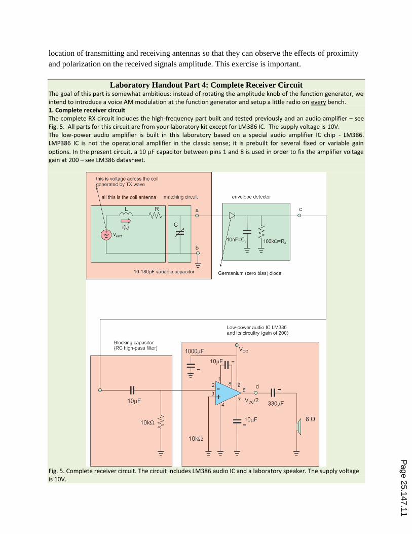
Laboratory Handout Part 4: Complete Receiver Circuit The goal of this part is somewhat ambitious: instead of rotating the amplitude knob of the function generator, we intend to introduce a voice AM modulation at the function generator and setup a little radio on every bench. 1. Complete receiver circuit The complete RX circuit includes the high-frequency part built and tested previously and an audio amplifier – see Fig. 5. All parts for this circuit are from your laboratory kit except for LM386 IC. The supply voltage is 10V. The low-power audio amplifier is built in this laboratory based on a special audio amplifier IC chip - LM386. LMP386 IC is not the operational amplifier in the classic sense; it is prebuilt for several fixed or variable gain
options. In the present circuit, a 10 F capacitor between pins 1 and 8 is used in order to fix the amplifier voltage gain at 200 – see LM386 datasheet.
Fig. 5. Complete receiver circuit. The circuit includes LM386 audio IC and a laboratory speaker. The supply voltage is 10V.
Page 25.147.11

2. Circuit assembly and radio link 1. Assembly the audio amplifier circuit on the remaining (right) side of the second protoboard. It is powered
by a 10V single power supply (limit current to 0.5A). Bypass the supply with a 1000µF capacitor (rail to rail) - see Fig. 5. Use the class speaker (in a black box).
2. Turn power supply on. Turn the transmitter on. The speaker should generate a quiet white noise. If this is
not the case (your computer screen, or cellphone, or etc. may generate a plenty of RF noise), put a 10 resistor in series with the 10µF capacitor between pins 1 and 8.
3. Turn the amplitude of the function generator to a minimum. 4. Now, you need to setup amplitude modulation at the transmitter. Use TAs help if you have any questions.
To do so: a. Push the button MOD/ON. b. Push the button MOD/EXT. c. Pull out MOD/DEPTH knob and rotate it all the way clockwise. d. Connect the cable from the back of the function generator to audio plug from your PC. e. Start play a sample audio clip “Sleep away” by Robert Acri. f. Slowly increase the amplitude of the function generator (transmitter) until you hear quiet
decent-quality music transmitted wirelessly.
The complete receiver circuit, including the audio amplifier, is shown in Figure 7. This circuit
and the transmitter circuit are shown together in Figure 8. All students (out of the pool of eighty
in one class, and one hundred and sixty three in another class) were able to successfully transmit,
receive, demodulate, and play an audio clip. However, a part of them (about twenty students)
needed extra time to complete the project.
According to students’ responses, this was the most interesting lab from total six (first class) or
seven (second class) laboratory projects given in class.
Figure 7: Complete RX circuit with audio amplifier
Audio
amplifier Parallel LC
receiver and
envelope detector
Page 25.147.12

Figure 8: Transmitter and receiver circuits set up to transmit, receive, and play sound file
from computer
Laboratory Organization, Common Mistakes, and Reception
Every class was subdivided in a number of laboratory sessions with 30 to 36 students in each
section (15 to 18 laboratory benches). Students were asked to complete this laboratory in a
single three hour laboratory session. A total of 300 students in 9 different laboratory sections
from two different classes participated in this laboratory activity. Students worked in groups of
two. The laboratory staff included 3 TAs. Generally, the laboratory was well received by both
the students and the TAs, although there were some challenges that should be addressed in future
implementations of this laboratory. Most common mistakes observed by the TAs included:
1. Running ground connections from the transmitting board to receiving board. This reflects
a fundamental misunderstanding of the concept of a ‘wireless’ circuit;
2. Improper and/or inaccurate use of the external modulation function of the function
generation;
3. Breaking the leads of the RX coils. The coils used were exceedingly delicate. On
average, 3-6 such coils were broken per laboratory section;
4. Ground rails problems with the LM386 audio amplifier IC. We found that the two most
inner rails of the protoboard should be grounded, for the best audio quality.
The most common conceptual misunderstanding was related to the role of the series/parallel
LCR circuit. While the series LCR circuit for the transmitter was used to maximize the coil
current, the parallel LCR circuits for the receiver was intended to maximize the output voltage.
Some of the students struggled to understand this concept. In addition, some of the students had
trouble understanding the meaning of the internal resistance of the coil in the circuit diagram.
TX circuit RX circuit with audio amplifier
Page 25.147.13

Conclusion
This paper presents laboratory materials that enabled students in an introductory ECE class to
build, observe, and understand a simple and reliable RF transmitter and receiver. The design is
simple enough to be consistently functional in an introductory laboratory environment and
performed well on student bread boards. This approach is repeatable, affordable, and provides
the students with an effective hands-on demonstration of a wireless link. The experiment was a
successful attempt to stimulate interest and learning in an introductory ECE class for both majors
and non-major students.
More sophisticated (and perhaps more expensive) radio laboratories are available – see [3]-[7].
Bibliography
1. S. Makarov, R. Ludwig, and S. Bitar, Electric Circuits and Circuit Components, Wiley Custom, Hoboken, NJ,
2011, ISBN 978-1-118-23356-8.
2. Laboratory #6, ECE2010-Intro to ECE, ECE Dept., WPI 2011-2012.
3. Online: http://courses.cit.cornell.edu/ee476/FinalProjects/s2010/pel29_slp56/pel29_slp56/index.html
4. Online: www.engr.uconn.edu/ece/.../projects/ecesd21/final-report-291.pdf
5. Online:
http://web.eecs.utk.edu/~snaciri/courses/ece342/project2/Project%20%232%20Report%20ECE%20342.pdf
6. Online: http://www.ece.vt.edu/ugrad/viewcourse.php?number=4676-149
7. Online: http://www.ik4hdq.net/doc/testi/HRL.pdf
Page 25.147.14