An Alternative Scheme for Chiron Fiber and Slicer Mode Data

Reductions

Frederick M. Walter

Stony Brook University

27 September 2017

update: 7 February 2018

Chiron (Tokovinin et al. 2012) is a stable high-throughput bench-mounted echelle spectrographfed by the 1.5m telescope on Cerro Tololo, operated by the SMARTS partnership. Three years ofexperience with Chiron, observing types of objects that Chiron was never designed to observed,have revealed some deficiencies in the standard data processing. I discuss here a new data reductionscheme for data obtained in the fiber and slicer modes. This provides different treatments of thelocal background and cosmic ray rejection, permits Gaussian extractions in addition to boxcarextractions, extracts 13 additional orders (down to about 4085A), and provides more order overlapand flatter orders. This may enable new and different kinds of science from the Chiron spectrograph.

1

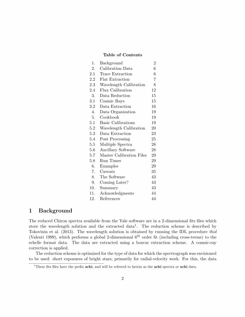
Table of Contents

1. Background 22. Calibration Data 6

2.1 Trace Extraction 62.2 Flat Extraction 72.3 Wavelength Calibration 82.4 Flux Calibration 123. Data Reduction 15

3.1 Cosmic Rays 153.2 Data Extraction 164. Data Organization 195. Cookbook 19

5.1 Basic Calibrations 195.2 Wavelength Calibration 205.3 Data Extraction 235.4 Post Processing 255.5 Multiple Spectra 285.6 Ancillary Software 285.7 Master Calibration Files 295.8 Run Times 296. Examples 297. Caveats 358. The Software 439. Coming Later? 43

10. Summary 4311. Acknowledgments 4412. References 44

1 Background

The reduced Chiron spectra available from the Yale software are in a 2-dimensional fits files whichstore the wavelength solution and the extracted data1. The reduction scheme is described byTokovinin et al. (2013). The wavelength solution is obtained by running the IDL procedure thid(Valenti 1999), which performs a global 2-dimensional 6th order fit (including cross-terms) to theechelle format data. The data are extracted using a boxcar extraction scheme. A cosmic-raycorrection is applied.

The reduction scheme is optimized for the type of data for which the spectrograph was envisionedto be used: short exposures of bright stars, primarily for radial-velocity work. For this, the data

1These fits files have the prefix achi, and will be referred to herein as the achi spectra or achi data.

2

reductions appear to work well. The radial velocities are certainly very stable.The extracted spectra (orders m=64-123)2 are divided by a flattened flat spectra, preserving

the gross echelle response. While orders m=126-138 (roughly 4100-4600A) also fall on the detector,they are not extracted. Furthermore, over 225 points well off the blaze are trimmed from orders.Exclusion of lower S/N data and retention of the blaze function makes sense for high precisionradial velocity data analyses, but I am interested in something completely different.

I have been using Chiron in a way that was probably never envisioned by its creators: synopticobservations of galactic novae. The challenges with the novae are many-fold. While bright atdiscovery (typically 10th mag, but up to 3rd mag), they fade: we follow them down to V∼18 insome cases (at which point essentially all the flux is in emission lines). This is below the nominalsensitivity of the acquisition camera, and so presents some challenges for the telescope operator.Other challenges arise from the fact that we use 10-30 minute exposures, so there is significantbackground and numerous cosmic rays. Finally, nova spectra are dominated by broad emissionlines, with FWZI up to 10,000 km/s. Background determination is non-trivial when the emissionline is broader than the echelle order!

In examining the extracted spectra (the achi*.fits files) I noticed the presence of narrow “ab-sorption features” (figure 1) near the tops of some of the emission lines in some of the novae.Originally I thought that this might be a new phenomenon attributable to our unprecedented high-resolution synoptic coverage, but some of the physics failed to make sense. My conclusion was thatat least some of these “features” might be due to incorrectly subtracted cosmic rays3, but furtherexamination suggests a more insidious problem: in some cases the bright emission lines themselveswere being treated as cosmic rays, and being removed4.

At that point I decided it was time to look into re-extracting the spectra. The code describedhere, written in IDL, does just that. It allows the user to re-extract the data, using both boxcar and(optionally) Gaussian extraction techniques. It extracts all the spectral points along the order, and75 orders, from m=64 through m=138 (74 orders starting at m=65 in the case of the slicer mode).This now-accessible spectral region is illustrated in figure 2. The broader wavelength coveragerequires a new wavelength calibration. A two-step cosmic ray masking is employed, and inter-orderbackground is subtracted.

The inputs for all the code described below are the chi*.fits raw data files.

2in general, when I refer to echelle orders in this document I refer to the index in the extracted two-dimensionalarray. This runs 0-n, where n is 73 or 74 for, respectively, slicer-mode or fiber-mode extracted data. Extracted orderi corresponds to physical order m=138 − i. The Yale extractions in the achi files run from 0-58, or physical ordersm=123 to 64.

3First suggested by U. Munari in the case of an apparent narrow reversal in Hα on one occasion in N Oph 2015.4Sometimes being slow to publish has its benefits.

3

Figure 1: Order 10 of achi150728.1127.fits. The target is the nova N Sgr 2015b. The emissionline is Fe II λ4921. The narrow dropouts are an artifact of the standard data reduction process.

4

Figure 2: What you’ve been missing. Orders 124-138 in a slicer-mode spectrum of η Car. Theextracted data have been flux-calibrated, and the orders have been spliced. The strong broad linesare Hδ λ4101A and Hγ λ4340A. Narrow blueshifted wind absorption is visible in both lines. Thenarrow emission lines are mostly Fe III.

5

Table 1: Calibration File Names

description Fiber-mode Slicer-mode Format

flat field image quartz.fits slquartz.fits * x xlentrace extraction trace yymmdd.sav sltrace yymmdd.sav xlen x Nord

extracted flats flats yymmdd.sav slflats yymmdd.sav xlen x Nord

extracted ThAr spectrum tharyymmdd.sav sltharyymmdd.sav xlen x Nord

wavelength solution yymmdd cfits.sav slyymmdd cfits.sav see table 2

notes:yymmdd is the civil date the data were obtained.files are in the calibration directory yymmdd cals.xlen is 1028 for the fiber and 4112 for the slicer.Nord is the number of extracted orders.

2 Calibration Data

There are 3 essential components to the calibration process:

• order trace extraction,

• flat extraction, and

• wavelength calibration.

The calibration process is similar for the fiber and slicer. Output calibration file names (table 1)are prepended with sl for slicer-mode data.

In preparation for the first two items, I co-add all the flat images taken in the appropriate modeand save that image to disk. I trim the data and subtract the overscan, using the regions definedin the fits header, prior to co-adding the images.

2.1 Trace Extraction

I use the coadded flat image for tracing the orders. Orders are aligned roughly vertically in theimages. I extract a subimage from y=500 to 550, where the middle of the chip is at y=513.5(multiply by a factor of 4 for slicer mode)), and collapse this into a vector using the medianfunction. I identify the Nord highest peaks (Nord=75 for the fiber and 74 for the slicer because oforder crowding at the red end). I test for missing orders and discrepant peaks, and identify thecentral positions of the orders. I trace these orders by centroiding the sum of 21 points centeredevery 10th point, and then fit this with a third order polynomial. The trace is stored in a xlen xNord array, which is written into an IDL save file (table 1) in the calibration data directory.

6

The trace extraction in fiber mode is clean because the orders are well-separated amd cleanlypeaked. This is not the case for the slicer. The cross-order profile is broad and triple-peaked. Iidentify the center of the order as being half-way between the minima on either side. Crowding ofthe orders at the red end (low order numbers) complicates matters, to the extent that I chose toignore order 64.

I also determine and save the width of the trace, for use in doing the boxcar extractions of thedata.

Because of the stability of the instrument, it is not necessary to extract a new trace each night.I find that using a master trace file, shifted as necessary in the cross-dispersion direction, suffices.

2.2 Flat Extraction

Flats are extracted two ways: boxcar extraction and Gaussian extraction. These techniques areoutlined below.

2.2.1 Boxcar Extraction

In this scheme, the data within ±wid pixels of the location of the trace at that Y position aresummed. The width of the fiber-mode extraction slit is ±3 pixels (set empirically). If fiber-mode,background is extracted on either side of the flat with a width set by the distance to the adjacentorders, less twice the extraction slit width. Following extraction, the two background spectra arefiltered to remove discrepant narrow features, and averaged. This is not possible for the slicer-mode except at the bluest wavelengths because of order-crowding. Rather, a global background fitbetween the orders is subtracted prior to the data extraction.

Because I keep track of the counts in the extracted spectrum and the background regions, Ikeep track of the

√N statistics and propagate the errors. The errors are stored as a S/N vector

because this is invariant when the fluxes are scaled.

2.2.2 Gaussian Extraction

In principle, extraction using the PSF can be optimal because cosmic rays and other defects willdeviate from the “known” profile. In practice, here I fit cuts across the spectrum with a Gaussianprofile, which is probably not the appropriate functional form. Because the closeness of the orderscan make it hard to constrain the background, I simultaneously fit three adjacent orders, except forthe first and last orders. where I only fit two. There are 12 free parameters (3 in the backgroundand three in each Gaussian). The fits to the outlying orders are discarded. The background isextrapolated under the central Gaussian. The relevant parameter is the analytic integral of theGaussian (which is presumably less affected by outlying points than is a straight summation of thedata).

The fitting is done using the mpfitfun (Markwardt) function with constrained fits. The initialfit is made to the sum of the 5 pixels at the center of the image (Y=514). Subsequent fits going

7

outward towards the top and bottom of the image use the previous fit as initial estimates. Theposition of the Gaussian is constrained to deviate from the previous fit by less than 1 pixel, and thewidth is constrained to deviate by less than 20%. Note that because the initial estimates dependon the previous fit, the solution can run away and settle on another order. This is not a problem forthe flats or for bright sources, but can be for faint objects. Therefore I have an optional iterativefitting process, where the position and width of the initial extraction are forced to those of thetrace extraction. In the second iteration these constraints are relaxed (see §3.2), with the positionfree to move by ±0.5 pix, and the width free to vary by ±10% from the values from the fit to thetrace. This reduces the likelihood that the solution will run away.

Gaussian extraction is probably not possible for slicer-mode data.

2.2.3 Comparison of Extractions

The boxcar- and Gaussian-extracted flats agree with each other (to within a normalization factor)to better than 1%, although there is significant structure (see figure 3). The structure correlateswith the width of the Gaussian fit across the order.

The boxcar extraction is flatter, relative to a low order polynomial, by a factor of 2, thanis the Gaussian extraction, so at first look it seems that the boxcar extraction is to be preferred.However, because of the stability of the instrument, the structure in the Gaussian flat largely cancelsout (figure 4), and the two extractions are comparable, even for reasonably high S/N spectra. Inprinciple the Gaussian extraction provides better cosmic-ray rejection, but it also takes significantlylonger to run (see §5.8).

Division by the flat, rather than by the flattened flat, yields a reasonably flat extracted order(Figure 5) which simplifies flux-calibration and order-splicing. Short of that, measurements ofspectral features are often easier on flat continua.

2.3 Wavelength Calibration

I was unable to get good wavelength solutions using the thid code. Eventually I decided to do awavelength solution the old-fashioned way. I selected one order and, using the thid solution as astarting point (see §5.2), obtained a wavelength solution. One can also use the wavelength solutionin the appropriate achi file for a starting point. Then it becomes a matter of identifying the correctwavelengths and fitting the data positions of the lines. I fit these with a polynomial. Using theproperties of the echelle, that mλ is constant as a function of the Y coordinate between the orders,I made an initial wavelength solution for each order, and then edited each order, removing blendsand weak lines. The air wavelengths of the lines come from thid data.xdr.

My master solution, derived for the fiber on the night of 150728, contains some 1300 lines in 75orders. The RMS scatter in the solutions for each order are good to better than 1 km/s.

This solution can then be migrated to other dates, doing a cross correlation of the “good” linelist with the extracted Th-Ar spectrum to generate a gross shift, and then automatically re-fitting

8

Figure 3: The normalized ratio of the boxcar-extracted to the Gaussian-extracted flat for order108. The green trace is the scaled width of the Gaussian used to extract the flat. They track well,with the larger ratio (less flux in the Gaussian extraction) when the fit is broader. This occurswhen the trace is centered between two pixels. I suspect this is attributable to the non-Gaussianityof the PSF. In any event, the effect seems to divide out (see figure 4).

9

Figure 4: The ratio of the boxcar-extracted to the Gaussian-extracted spectra, after flat division,for order 108 of chi131014.1143 (µ Col). The RMS scatter of the ratio is 0.6%. The median is0.999; no normalization has been applied. The structure visible in the flat ratio (figure 3) is greatlyreduced. The SNR of the spectrum, from counting statistics alone, peaks about 900, and exceeds500 between pixels 250 and 850. Within this region the RMS is about 0.4%, comparable to the0.3% expected from counting statistics alone.

10

Figure 5: A particularly boring part of the spectrum of the O9.5V star µ Col, a spectrophotometricstandard. Note that division by the actual flat extraction yields a very flat spectrum.

11

Table 2: ths Structure Tags

Tag Format Description

cfits dblarr(9) coefficients of polynomial fit (up to 8th order)sdv float standard deviation of polynomial fit: units=pixnp integer Number of lines fitm integer physical order number (138 - 64)pixfit fltarr(np) X pixel of fit positionwavfit fltarr(np) air wavelength of fit positiondiff fltarr(np) wavelength - fit wavelengthwid fltarr(np) Gaussian FWHM of linemlam dblarr(3) mλ for pixels 0, 514, and 1027xcut intarr(2) currently unusedmres double mean resolution E/δE

the individual lines. The goodness of the solution is estimated by plotting mλ as a function ofX-position for all the lines fit. There is an irreducible order-dependent scatter of up to ± 60Ain mλ after subtracting the best fit third-order polynomial. The 150728 solution maps well intoall the Th-Ar spectra obtained (starting with 120324) - a strong testament to the stability of theinstrument.

Verification of the wavelength solution is based on looking for significant deviations in mλ fromthat expected, and consequently in the length of the order in wavelength space. Deviant lengthsare generally due to poorly-constrained solutions near the ends of orders with few lines near theorder extrema. Refitting with a lower order polynomial usually fixes the problem.

The wavelength solution is written to an IDL save file (table 1). The file contains a structure,ths which has one element per order fit. The tags are listed in Table 2. Note that the pixfit, wavfit,diff, and wid tags are padded to 60 element arrays.

It is important to realize that, while I need a reliable wavelength solution, I do not need one withthe fidelity of the Yale solution. Consequently, I have neither examined nor tweaked the solutionson most nights for the best possible solutions. But they look pretty good (see figure 6).

For slicer mode I start with the fiber solution, and search for lines at the predicted pixel locationfor a quadrupled resolution. It seems to work - see figure 7.

2.4 Flux Calibration

Conversion from counts to flux requires observation of a flux-standard star under photometricconditions. Since many factors come into play (e.g., seeing, slit width, wavelength-dependent slitlosses, etc.), I use the flux-standard to establish the shape of the instrumental response. Absolute

12

Figure 6: The Na D lines in N Oph 2015 on 150728. There are few narrow lines in novae - theseare interstellar. The achi spectrum is in aqua. The wavelength solutions are in good agreement.

13

Figure 7: A comparison of the slicer mode spectrum of σ Ori using my reductions (black) and thespectrum from the achi file (blue) processed using the Yale reduction. This is a portion of order42 (order 27 in the achi file) containing the Na D1 line. The difference in slope is attributable tofact that I divide by the extracted flat, while the achi spectrum is not flattened. A heliocentriccorrection is applied to both spectra; fluxes are normalized to the median in the plotted region.The spectra match well; there is a wavelength offset corresponding to 0.4 km/s between the spectrathat could arise from many sources.

14

calibration (at least for a variable star) requires simultaneous photometry. I have used µ Col(HR 1996), a bright star

3 Data Reduction

3.1 Cosmic Rays

In most cases, I have taken single exposures in order to maximize S/N in a given time. This comesat the expense of contamination by cosmic rays. The propensity of the default reductions to flagand remove strong emission lines is a major motivation for this reduction effort.

There are two cases to consider: cosmic rays on or near the order, and those in the background.Cosmic rays in the background are the less serious issue. Filtering, and then averaging, the

background spectra on either side of the order efficiently removes most small-scale blemishes. Inthe Gaussian extractions I fit 4 interorder regions, ensuring that small features will have a minimaleffect.

However, most cosmic ray detection algorithms look for sharp edges, very much like the dis-persed spectrum, and this can cause difficulties. I originally tried a direct application of thela cosmic procedure (van Dokkum 2001), and found that it tended to chew up the spectra. Aftersome experimentation, I decided to pre-filter the data with a 1x5 median filter. This has the ben-eficial effect of removing sharp features in the dispersion direction, while only minimally reducingresolution for sharp features. Then an application of la cosmic seems to do a better job, but it stillhas trouble with the bright Hα emission line in many novae (and also with other narrow emissionlines). So I incorporated a keyword to let one ignore any masked data in the immediate vicinity ofHα.

Alternatively, the dcr (Pych 2004) algorithm can be used too, by specifying the dcr keyword inthe call to ch reduce. The user will need to install the dcr executable. A customized dcr.par file iswritten in the working directory. The THRESH, XRAD, YRAD, NPASS, and GRAD values can beset via keywords. I’ve modified the default values for XRAD and YRAD to 4 and 31, respectively.When dcr works, it gives about the same results as does la cosmic as implemented here, though itseems to miss more cosmic rays, especially in high S/N spectra. It may be possible to fine tunethe parameters to do a better job. dcr runs much faster than la cosmic. However, it seems to beunstable, in that varying the XRAD and YRAD can give wildly divergent results, including clearlyunphysical continuua. dcr seems to remove low points as well as high points, which can get it intotrouble near the ends of orders.

The data quality vector (see Tables 3 and 6) encodes pixels affected by cosmic rays, as well assaturated pixels.

If you have a spectrum with lots of narrow emission lines (as in a nebulosity), running ch reducewith the noclean keyword set prevents the code from interpreting narrow emission lines in thespectrum as cosmic rays. I have specific exceptions built in to prevent the code from interpretingnarrow telluric Na D and O I λ6300 emission as cosmic rays.

15

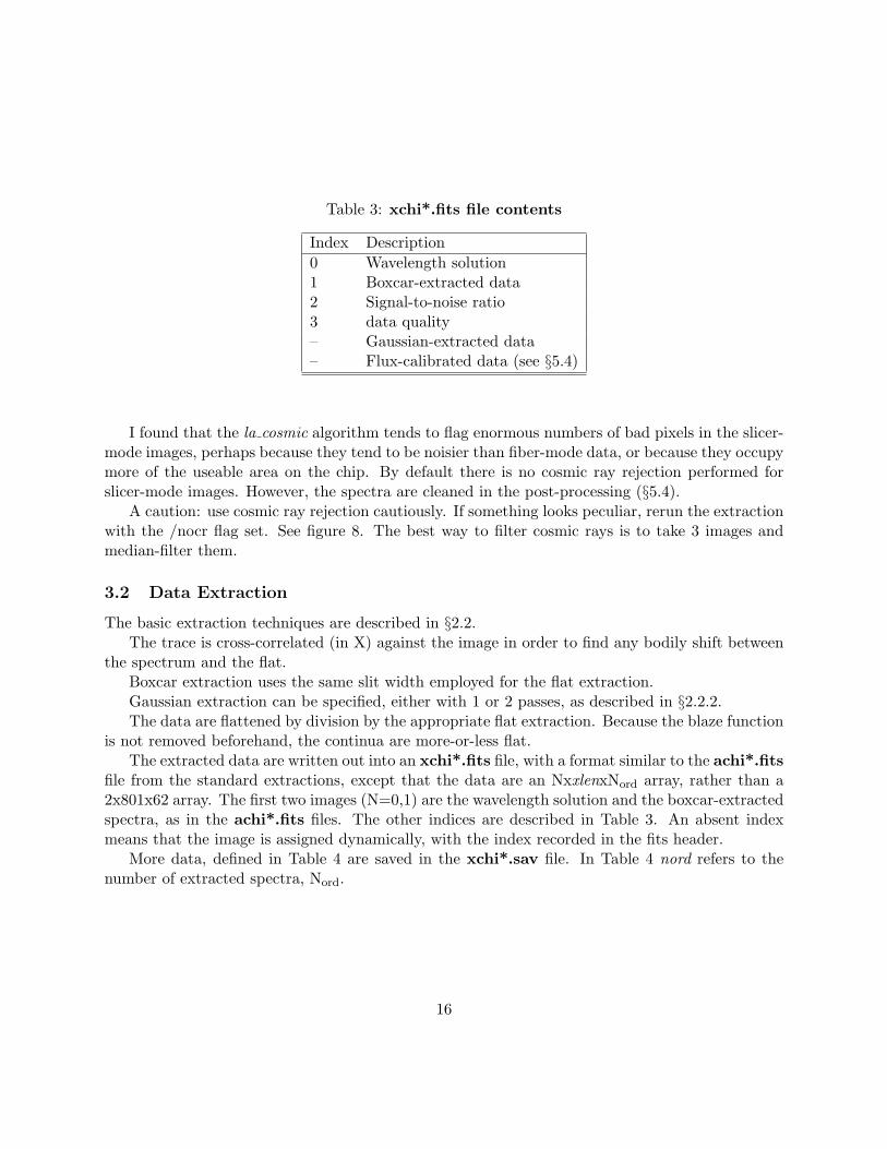
Table 3: xchi*.fits file contents

Index Description

0 Wavelength solution1 Boxcar-extracted data2 Signal-to-noise ratio3 data quality– Gaussian-extracted data– Flux-calibrated data (see §5.4)

I found that the la cosmic algorithm tends to flag enormous numbers of bad pixels in the slicer-mode images, perhaps because they tend to be noisier than fiber-mode data, or because they occupymore of the useable area on the chip. By default there is no cosmic ray rejection performed forslicer-mode images. However, the spectra are cleaned in the post-processing (§5.4).

A caution: use cosmic ray rejection cautiously. If something looks peculiar, rerun the extractionwith the /nocr flag set. See figure 8. The best way to filter cosmic rays is to take 3 images andmedian-filter them.

3.2 Data Extraction

The basic extraction techniques are described in §2.2.The trace is cross-correlated (in X) against the image in order to find any bodily shift between

the spectrum and the flat.Boxcar extraction uses the same slit width employed for the flat extraction.Gaussian extraction can be specified, either with 1 or 2 passes, as described in §2.2.2.The data are flattened by division by the appropriate flat extraction. Because the blaze function

is not removed beforehand, the continua are more-or-less flat.The extracted data are written out into an xchi*.fits file, with a format similar to the achi*.fits

file from the standard extractions, except that the data are an NxxlenxNord array, rather than a2x801x62 array. The first two images (N=0,1) are the wavelength solution and the boxcar-extractedspectra, as in the achi*.fits files. The other indices are described in Table 3. An absent indexmeans that the image is assigned dynamically, with the index recorded in the fits header.

More data, defined in Table 4 are saved in the xchi*.sav file. In Table 4 nord refers to thenumber of extracted spectra, Nord.

16

Figure 8: These panels illustrate the effects, both good and bad, of cosmic ray filtering singleimages. The lower panel shows how cosmic ray rejection is supposed to work. The black traceis the boxcar-extracted spectrum with cosmic ray detection turned off (/nocr); the green trace isthe same extraction with nominal CR rejection using the la cosmic software. A narrow positivedeviation, seen in black, is rejected (this results from setting spfitord=0; the default setting ofspfitord=2 finds and rejects this event). The upper panel shows what happens when a real narrowfeature is mis-identified. The default extraction produced the green trace. Note the absence ofthe strong interstellar Na D1 line. The magenta trace is the extraction run with CR rejectionand with the /noclean keyword set. Points flagged as bad by la cosmic are set to zero. If the/noclean keyword is not set the flagged points are interpolated over (the green trace). Setting the/nocr keyword results in the black spectrum, and a normal-looking pair of Na D lines. This is afiber-mode spectrum of V339 Del shortly after maximum.

17

Table 4: xchi*.sav file contents

Variable format description

FILELOG structure header informationH strarr(*) FITS headerMASK bytarr(*, xlen) mask image from la cosmicTHS structure(nord) defined in Table 2XFITS fltarr(xlen,nord) traces

Boxcar Extraction ParametersBACK fltarr(xlen, nord) background spectraBDATA fltarr(xlen, nord) net extracted spectrumBDQ intarr(xlen, nord) data quality flagsBDX fltarr(xlen, nord) extracted, flat-fielded spectraSNR fltarr(xlen, nord) SNR for BDATA, BDXWID fltarr(xlen, nord) extraction width = 2*wid+1

Gaussian Extraction ParametersGDATA fltarr(xlen, nord) net extracted spectrumGDQ intarr(xlen, nord) data quality flagsGDX fltarr(xlen, nord) extracted, flat-fielded spectra

OtherFN fltarr(xlen, nord) fluxed extracted spectrumDS fltarr(xlen, nord) data removed in spectral cleaning

18

4 Data Organization

All data and calibration data are stored in the directory chirondata. The cshell definition is

setenv chirondata YourDataDirectory

Create a subdirectory cal under chirondata.Tar files downloaded from the Yale archive should be saved and unpacked in the chirondata

directory. Each night will be in a subdirectory named YYMMDD, the observation date.Calibration data should be downloaded to and unpacked in chirondata/cal. There will be a

series of directories of the form YYMMDD cals.Extracted and derived calibration data are saved in the chirondata/cal subdirectories. Extracted

spectra are saved in the chirondata subdirectories.All procedure file names are lower case; on occasion in this document I have spelled them with

mixed cases to improve readability.

5 The Cookbook

The code is written in IDL, and was tested under version 8.1. The process of calibrating andreducing a night’s data is easily divided into three parts5.

5.1 Basic Calibrations

The data must be in the chirondata/cal/YYMMDD cals directory (see §4). Ch Cals reads thecalibration data, and

• co-adds the flat images,

• traces the orders in the flat images,

• extracts and writes the flat orders,

• extracts and writes the Th-Ar spectrum, and

• computes the wavelength solution.

The files written in the process are listed in table 1.

Ch_Cals: reduce Chiron calibration images

* calling sequence: Ch_Cals,day

* DAY: 6 digit string (yymmdd); required

5Omnes data in tres partes divisa est.

19

*

* KEYWORDS:

* DOGAUSS: set to enable Gaussian extraction of flat

* EXAMINE: set to examine each extracted order (sets plt)

* FIXWID: sets fixed extraction width

* FORCE: set to remake the quartz.fits file

* MKTRACE: set to make new trace (2 to lookup w/o shifting)

* MODE: default=fiber

* NOWAVCAL: if set, skip wavelength solution migration

* PLT: set to follow the extractions by plotting the extracted orders

* REFTHAR: index of reference ThAr spectrum, def=first

* SLICER: shorthand for mode=’slicer’

* USEFLAT: set to use pre=extracted flat for this day

* WCALONLY: set to redo ch_migratewcals

You must run Ch Cals independently for each observing mode you wish to calibrate. Set thedogauss keyword only if you intend to do Gaussian extractions in fiber mode. Gaussian extractionis slow because it requires fitting a Gaussian profile at each point in each order. Gaussian extractionis not enabled for slicer data.

Unless the keyword nowavcal is set, the default wavelength solution will be migrated to thisday, using the Th-Ar spectrum for this day. See §5.2 for more details.

If multiple Th-Ar observations exist, all images are cross correlated against the reference ThArimage (by default, this is the first of the ThAr images; change this with the refthar keyword)). Theresulting pixel shifts are saved in the extracted ThAr .sav file. The instrument is stable: the driftsover the night of 21 July 2017 (fiber mode) are shown in Figure 9.

Set the plt keyword to see the extracted flat orders. Set the examine keyword to pause after eachorder is plotted. While paused, type “z” to get an IDL prompt; type any other key to continue.

The wrapper Do ChCals runs Ch Cals on multiple directories. You can use Ch CalStatus to listdirectories that have yet to be calibrated.

5.2 Wavelength Calibration

For many of these routines, you will need the Th-Ar line list in thid data.xdr. This file shouldbe saved as chirondata/cal/thid data.xdr. You will also need the extracted ThAr save file filegenerated by ch cals. The wavelength solutions are stored inchirondata/cal/YYMMDD cals/xYYMMDD cfits.sav, where x is sl for slicer spectra andnull for fiber spectra.

These routines use a number of common subroutines. In plwfit, commands are entered by singlekeystrokes as defined in Table 5.

The basic routines used in wavelength calibration are:

20

Figure 9: The drift in pixels over the course of a night of the Th-Ar spectra in fiber mode. Thedrift correlates well with various instrumental temperatures. While the drift is systematic, and isaccounted for in the extraction software, it is also insignificant for many purposes. Chiron is stable.

21

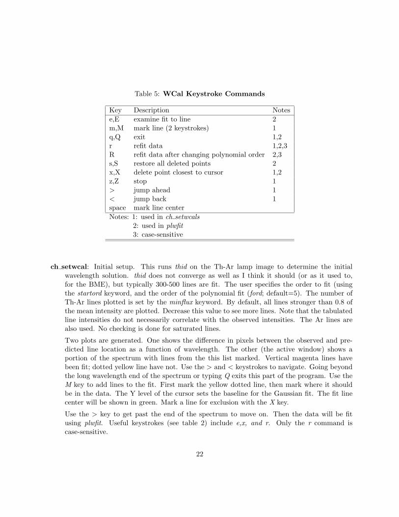
Table 5: WCal Keystroke Commands

Key Description Notes

e,E examine fit to line 2m,M mark line (2 keystrokes) 1q,Q exit 1,2r refit data 1,2,3R refit data after changing polynomial order 2,3s,S restore all deleted points 2x,X delete point closest to cursor 1,2z,Z stop 1> jump ahead 1< jump back 1space mark line center

Notes: 1: used in ch setwcals2: used in plwfit3: case-sensitive

ch setwcal: Initial setup. This runs thid on the Th-Ar lamp image to determine the initialwavelength solution. thid does not converge as well as I think it should (or as it used to,for the BME), but typically 300-500 lines are fit. The user specifies the order to fit (usingthe startord keyword, and the order of the polynomial fit (ford; default=5). The number ofTh-Ar lines plotted is set by the minflux keyword. By default, all lines stronger than 0.8 ofthe mean intensity are plotted. Decrease this value to see more lines. Note that the tabulatedline intensities do not necessarily correlate with the observed intensities. The Ar lines arealso used. No checking is done for saturated lines.

Two plots are generated. One shows the difference in pixels between the observed and pre-dicted line location as a function of wavelength. The other (the active window) shows aportion of the spectrum with lines from the this list marked. Vertical magenta lines havebeen fit; dotted yellow line have not. Use the > and < keystrokes to navigate. Going beyondthe long wavelength end of the spectrum or typing Q exits this part of the program. Use theM key to add lines to the fit. First mark the yellow dotted line, then mark where it shouldbe in the data. The Y level of the cursor sets the baseline for the Gaussian fit. The fit linecenter will be shown in green. Mark a line for exclusion with the X key.

Use the > key to get past the end of the spectrum to move on. Then the data will be fitusing plwfit. Useful keystrokes (see table 2) include e,x, and r. Only the r command iscase-sensitive.

22

ch tweakwcals: use to tweak an existing wavelength solution for one order. Call it asch tweakwcals,YYMMDD,order=x,mode=mode.

ch migratewcals: use to migrate a wavelength solution from one day to another.

* Ch_MigrateWcals - migrate one Chiron wavelength solution to a different day

* calling sequence: Ch_MigrateWcals,date

* DATE: date in format YYMMDD, no default

* Ch_Cals must have been run for this date

*

* KEYWORDS:

* AUTOFIT: def=2; 1 to examine each fit

* EXCLSIG: automatic line exclusion, def=2.5 sigma from initial fit

* MINFLUX: def=0.8 of mean of Th-Ar intensities

* MODE: default=’fiber’

* ORDERS: set for select orders

* REFFIT: reference fit date (YYMMDD), def="chiron_master_wcal"

* THRESH: threshold counts in line for autofit, def=20

ch examinewcals: non-interactive examination of the solution. It plots the deviations of the fitmλ after subtracting a third order polynomial. Outliers are flagged, and orders that are toolong or too short are identified so they can be refit. Do this by runningch examinewcals,/redord, which uses ch tweakwcals,/redord on the flagged orders.

ch extendwcals: use to apply the solution for one order to another order on the same night.

ch wcalsummary: generates a summary of each wavelength solution (one line per order). Thelast column, the mean resolution, gives a good data quality indicator. It should be about28,000 for fiber-mode data, and 78,000 for slicer-mode data.

Once you have a master wavelength calibration, you should be able to use ch migratewcalsand ch examinewcals to calibrate all other days.

5.3 Data Extraction

The calibration files including a wavelength solution, must exist before data can be reduced6. Thedata must be in the chirondata/YYMMDD directory (see §4). To reduce a full night’s data, merelyrun ch reduce,YYMMDD. To reduce a particular spectrum, type ch reduce,YYMMDD,file=xxxx,where xxxx is the 4 digit file number (chiYYMMDD.xxxx.fits). The file number xxxx can beeither a string or an integer.

6You can calibrate the data using cal data from another night by specifying the date in the caldate keyword.

23

Ch_Reduce: reduce raw Chiron Spectra

* calling sequence: Ch_Reduce,date

* DATE: 6 digit string (yymmdd); required

*

* KEYWORDS:

* CALDATE: set to date of calibrations, if not date

* Do2: set to coadd and extract a pair of images

* Do3: set to coadd and extract a triad of images

* DOGAUSS: 1 or 2 for Gaussian extractions

* EXAMINE: set to examine each extracted order (sets plt)

* FILE: name of file; def = all

* MODE: default=fiber

* NOCLEAN: set to skip extrapolation over bad points

* NOCR: set to skip CR filtering

* NOHAMASK: set if H-alpha is in emission

* NOPROC: set to skip post processing

* NOSAVE: set to run code but to not save the data; stops when done

* NSIG: sigma cut for replacing bad points in Gauss fit. Not yet implemented.

* OPTIMUM: set for optimum extraction. Not yet implemented.

* PREFILTER: 1xn filter, def=5

* SPFITORD: background order for ch_cleansp; def=2

* STARTORD: starting extraction order, def=0

* UPDATE: set to update single order

ch reduce options:

• If the keyword file is not specified, all files in the specified mode will be extracted indepen-dently, If file is specified (as either a string or integer), only that file is reduced.

• The boxcar extraction is the default.

• A Gaussian extraction is specified (in addition to the boxcar) by setting the dogauss keywordto 1 or 2, for either single pass unconstrained fit or a constrained double pass fit (§2.2.2).Note that this option significantly slows down the execution time.

• If there is a strong Hα emission line, the cosmic ray filtering may wipe it out. See figure 11for an example. This will happen in ch reduce unless the nohamask keyword is set. Thisprevents the code from identifying the top of the Hα line as a defect, unless saturated.

• The clean algorithm identifies the pixels flagged as bad and interpolates over them. Use thenoclean keyword to turn this off. All bad pixels are identified in the bdq vector (see Table 6).

24

Table 6: Data Quality Flag

Flag Description

1 pixel flagged by la cosmic in lower background slit2 pixel flagged by la cosmic in upper background slit4 extracted data interpolated over single flagged pixel along spectrum8 extracted data interpolated over single flagged pixel across spectrum16 pixel flagged by la cosmic in extraction slit32 gaussian flat = 064 flagged in ch cleansp512 saturated pixel

• set nocr to see what happens in the absence of cosmic ray filtering. nocr is the default forslicer mode.

• Use the update keyword to reprocess a single order. Set update to the order number (0-74).

The output from Ch Reduce is the files xchiYYMMDD.xxxx.fits and xchiYYMMDD.xxxx.sav,as described in §3.2.

5.4 Post Processing

Ch reduce writes out the extracted, flat-fielded counts spectrum. Post-processing consists of a.)spectral cleaning b.) flux-calibration, and c). creating a spliced one-dimensional spectrum.

Spectral Cleaning: A final round of spectral cleaning is performed here. Points that exceed a setnumber of standard deviations above a local background are flagged as as outliers. The localbackground is a polynomial fit to a region100 points wide. The order of the polynomial is setby the keyword spfitord. The threshold is 5σ for orders up to 60, 6σ for orders 60-67, and7σ for the reddest orders. Flagged points are interpolated. Turn this off with the nospcleankeyword.

The lower panel of figure 8 shows that the spectral cleaning algorithm may not filter outsmall events (cosmic rays or hot pixels) above a variable background when spfitord is 0 or 1.Re-read section §3.1

Flux Calibration: I calibrate the response using a fiber-mode spectrum of µ Col obtained on131014, or a slicer-mode spectrum of µ Col obtained on 131008. In each order the counts areratioed to the modeled spectrum7. The modeled spectrum is low resolution: I smooth over

7available at https://www.eso.org/sci/observing/tools/standards/spectra/hr1996.html

25

Figure 10: The flux-calibrated slicer spectrum of µ Col (image chi131008.1140).

Balmer lines. The conversion (Fλ/count) is saved in fluxcal fiber.sav or slfluxcal fiber.savin the chirondata/cal directory.

There are issues with the calibration near the telluric A and B band heads.

In order to make your own master flux calibration file, you must run ch reduce,/noproc onthe flux calibrator. Then run ch mkfluxcal. Specify the observing mode, data, and file withthe MODE, DATE, and REC keywords. You will need to change the defaults.

The procedure ch calflux is used to convert the counts spectrum to a flux spectrum. To savethis to disk, use ch xupdate,flux=1. The xchi*.sav and xchi*.fits files are updated. Thearray in the fits file is expanded. Rd Chiron extracts this as d.f in the d structure.

Note that spectroscopic flux calibration is predicated on the assumptions that both the cali-

26

Table 7: Ch Splice Output Structure

Tag Type Size Description

W DOUBLE Array[xlen, Nord] xchi 2-D wavelength vectorS DOUBLE Array[xlen, Nord] xchi 2-D counts vectorE DOUBLE Array[xlen, Nord] xchi 2-D signal-to-noise vectorF DOUBLE Array[xlen, Nord] xchi 2-D flux vectorH STRING Array[] fits headerW1 DOUBLE Array[xlen2] spliced 1-D wavelength vectorF1 DOUBLE Array[xlen2] spliced 1-D flux vectorE1 DOUBLE Array[xlen2] spliced 1-D signal-to-noise vectorDQ DOUBLE Array[xlen2] spliced 1-D data quality vectorSPLICE DOUBLE Array[2(Nord)-1] splice pointsSKY FLOAT 0.00000 sky spectrum (not currently used)

brator and the target are observed under photometric conditions, and with equal slit losses.This is often not the case.

Order Splicing: Splicing of the individual orders is accomplished by the ch splice function, calledas z=ch splice(xfile), where xfile is the xchi*.fits file name or number. z is an expanded struc-ture described in Table 7. The output is a save file named object YYMMDD.xxxx.sav,where object is from the fits header (with all spaces removed).

The 1-dimensional wavelength vector is linear, with a bin size equal to the smallest in z.w, sothat no resolution is lost. The vector length xlen2 is about 82,000 points in fiber mode andabout 322,000 points in slicer mode. The flux and signal-to-noise vectors are interpolated tothis linear wavelength scale. The method of splicing is either to do a straight sum (keywordsum), to cut by the signal-to-noise vector (keyword cut, or to weight by the signal-to-noisevector (default).

When the data are weighed by the errors (signal/signal-to-noise), all negative points areexcluded as unphysical.

Because the splice regions are at the ends of the orders, they tend to have low S/N. Thefile chirondata/cal/ch deftrims.dat lists the empirically-determined “best” cuts, basedon visual inspection of the µ Col orders. You can change these with the trim keyword, whichis added to the defaults (subtracted from the RHS) . trim can be be a scalar, a 2-elementvector (left, right), or a full (2xNord) vector.

Setting the scale keyword will perform a scaling of the two spectra in the overlap region. Thisshould not be necessary, since the flux calibration serves the same purpose. Furthermore,

27

in regions where the flux calibration may be suspect (e.g., the edges of strong lines, or theterrestrial A and B bandheads), this may introduce an unwanted shift in the flux levels.

By retaining all xlen points in the orders, interorder gaps are eliminated through order 69(8260A) when using the default order trims). The user can override the number of pointsretained for splicing by specifying the trim or by editing ch deftrims.dat.

The flux calibration and the order splicing, as well as checking and updating the wavelengthsolution, are handled by the ch postproc procedure.

5.5 Multiple Spectra

Cosmic ray rejection is simpler, and more robust, when you have two or more spectra of an objectobtained on the same night under the same conditions. The routine ch reduce also handles multiplespectra of the same target.

In ch reduce, setting the do2 or do3 keywords will result in 2 or 3 consecutive images being coad-ded prior to extraction. Setting file to an N element array has the same effect for non-consecutivelynumbered files. Currently the code supports N up to 5.

With image pairs, cosmic ray rejection is handled by searching for excursions in the differenceimage that exceed a multiple (set by the keyword nsig) of the expected variance. With 3 or moreimages, the coadded image is the median at each point. After the coaddition, ch reduce runs as fora single image, with the exception that the output file names are numbered 9xxx rather than xxxx,where xxxx is the number of the first file.

See Figure 21 for an example of a coadded pair of deep exposures.There may be problems co-adding high S/N pairs or triads with different exposure times, or

which differ in instrumental throughput due to variable transparency of the sky. This is becausethe files are co-added prior to background subtraction.

5.6 Ancillary Software

In almost all cases, typing procedure,/help will bring up brief on-line help.

ch calstatus: check for the existence of calibration data.

ch sat: identify saturated pixels in chi*.fits image.

ch status: check for unreduced data.

ch xy: convert between pixel and order/wavelength coordinates.

comp chx: compare various extraction methods.

plch: quick plot of 1-dimensional Chiron spectra

28

rd chiron: read fits file, and convert to an IDL structure. Works for both achi*.fits andxchi*.fits files. Use the xfiles keyword to read a xchi*.fits file if both types exist.

5.7 Master Calibration Files

The following files are in chirondata/cal:

chiron master flats.sav A flat spectrum. It is advisable not to use this, but rather to extractthe flat on each individual night and use the local flats YYMMDD.sav file.

fluxcal fiber.sav Flux calibration for the fiber mode spectra.

chiron master trace.sav Traces. This is used by default unless mktrace is specified in ch cals.

chiron master wcal.sav The master wavelength calibration file which is migrated to and tweakedfor other nights.

ch deftrims.dat Default number of pixels to be trimmed from the orders prior to splicing.

The procedure ch cals writes the files specified in table 1 into the YYMMDD wcal directories.

5.8 Run Times

All run times refer to a Linux desktop running CentOS 6.7. The hardware is an Intel Core DuoCPU clocking at 3 Ghz, with 3.8 Gb of memory. The IDL version is 8.1.

Full calibration of a single night requires about 15 seconds for the fiber daya, and about 3 timesas long for slicer data. However, enabling Gaussian extractions in fiber mode increases the runtimeto about 19 minutes.

Boxcar extraction and post-processing of an image requires less than one minute.Extraction and calibration of a spectrum, including the Gaussian extraction, requires about

20-25 minutes for high S/N spectra, and up to 50 minutes for noisier spectra. The (lack of) speedis mostly attributable to my using mpfitfun to fit 12 free parameters to 1028 slices of the spectrumin each of Nord orders. This can probably be accelerated.

6 Examples

Here I present a few examples comparing my reductions with the Yale reductions. In all plots myreductions are in black. Red ticks at the bottom of the plot indicate pixels flagged as bad.

Figures 11 through 15 are 1800 second integrations taken of N Sco 2015 on 28 or 29 July 2015.The V mag was 15.0 at this time.

29

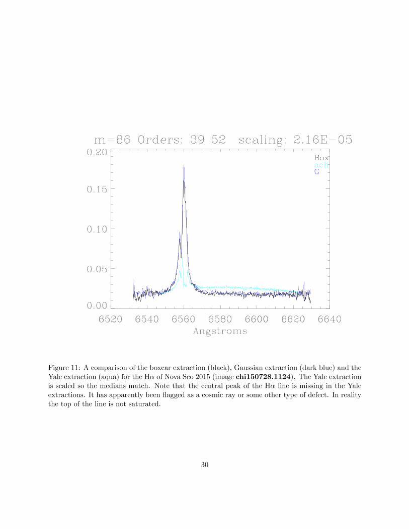
Figure 11: A comparison of the boxcar extraction (black), Gaussian extraction (dark blue) and theYale extraction (aqua) for the Hα of Nova Sco 2015 (image chi150728.1124). The Yale extractionis scaled so the medians match. Note that the central peak of the Hα line is missing in the Yaleextractions. It has apparently been flagged as a cosmic ray or some other type of defect. In realitythe top of the line is not saturated.

30

Figure 11 shows the effect of the cosmic ray detection algorithm on the peak of the Hα emissionline.

Figures 12 and 13 show the region of the sodium D lines, and illustrate the consequences ofsubtracting the instrumental background.

Figures 16 through 18 compare slicer-mode extractions. The target is η Car, which has lots offairly narrow emission lines. The comparison is with the Yale-extracted spectra after I haveflux-calibrated and spliced the orders. The absolute fluxes should be ignored; the spectraare scaled by their respective medians. Figure 16 is a region dominated by emission lines;figure 17 shows the Na D region, which is dominated by deep absorption. These figures howthat while the overall spectra are similar, there are artifacts attributable to idiosyncraciesof the reduction processes. The wavelength scales are not identical. Cosmic ray rejectionis not identical. Sharp features are dealt with differently. The two schemes agree well forlow-contrast spectral features.

Figures 19 through 20 are of V5668 Sgr (N Sgr 2015b). At this time the novae was near theminimum of its dust dip, but was still reasonably bright, at V =12.5. This is an 1800 secondintegration.

Figure 21 shows the quality of spectrum one can get on a faint object (V745 Sco at R > 16). Italso illustrates the quality of the order splicing.

Finally, figure 22 shows a series of slicer-mode spectra taken after the reopening/refurbishmentin July/August 2017. These spectra show the growth of the Hα emission line in the very slownova N Sct 2017 (ASASSN-17hx).

7 Caveats

The code was developed under IDL version 8.1, and in principle will run under version 7. It doesnot use widgets or object graphics. It does require the IDL Astronomy User’s Library8. Note thatsome of the procedures have the same names as built in IDL routines, including mean and gaussfit.Originally I did this to enhance the functionality or simplify the calls, so they were simple drop-ins.Not sure of that anymore9. So when you add this library to your IDL PATH, consider putting itfirst.

The Gaussian-extraction part of the code is slow. For now Gaussian extraction is turned off bydefault in ch reduce and ch cals.

8http://idlastro.gsfc.nasa.gov/9Yes, this is bad programming practice. But it would be a lot of effort to edit 30 years worth of homegrown code.

And I’m pretty sure I wrote my mean.pro before RSI did.

31

Figure 12: A comparison of the boxcar extraction (black) with the Yale extraction (aqua) for thesodium D line region of Nova Sco 2015 (image chi150729.1124). The Yale extraction is scaled sothe medians match. Note that the line strengths are much weaker in the Yale reduction, while theS/N is higher. This suggests that the background has not been subtracted in the Yale reductions(see figure 13). The emission line is He I λ5876. Multiple velocity components are visible inthe Na D1 and D2 lines. The low velocity components are galactic foreground; the blue-shiftedabsorption lines may be ejecta from the nova.

32

Figure 13: This is the same data as shown in figure 12, except that the data (black) are notflattened, and the background has not been subtracted. This provides a reasonably good match tothe Yale reductions (magenta).

33

Figure 14: Order 67, showing strong emission from the λ8498 component of the Ca II IR triplet.The line is not evident in the Yale reductions. The apparent strengths of the λ8446A O I line arealso very different.

34

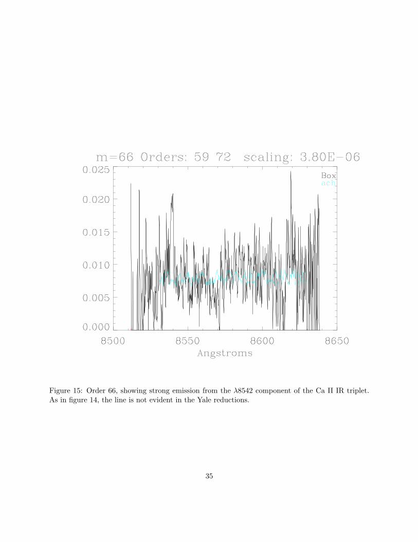
Figure 15: Order 66, showing strong emission from the λ8542 component of the Ca II IR triplet.As in figure 14, the line is not evident in the Yale reductions.

35

Figure 16: A region dominated by emission lines (mostly Fe III). In the lower plot, the black traceis from the new reductions while the magenta trace is the Yale extraction after flux calibration andorder splicing. The upper plot shows the ratio of the two. The dotted vertical line shows an ordersplice. The upper plot shows 3 artifacts. There are wavelength offsets in the λ5261A and 5275Alines, but the senses are different, suggesting that one wavelength scale is stretched relative to theother. The positive excursion in the ratio at 5274A is a cosmic ray or hot pixel not flagged in myreduction scheme (it is not designed to work well in highly non-linear regions). The 1% step at theorder splice at 5279A is in the new reduction scheme.

36

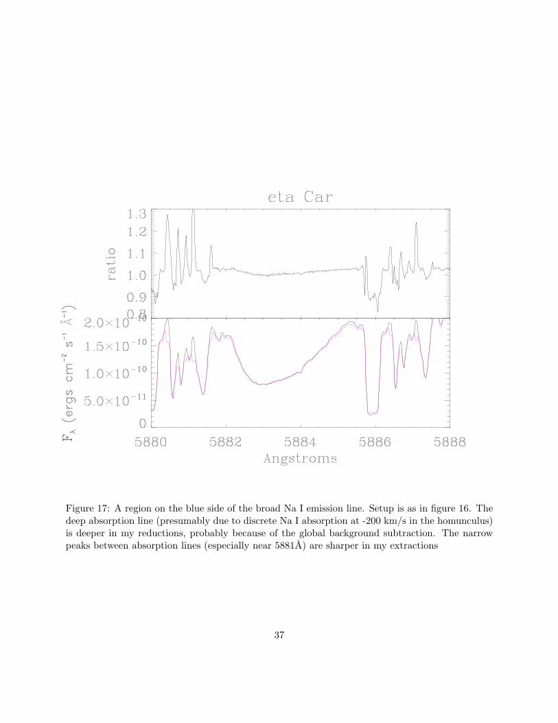
Figure 17: A region on the blue side of the broad Na I emission line. Setup is as in figure 16. Thedeep absorption line (presumably due to discrete Na I absorption at -200 km/s in the homunculus)is deeper in my reductions, probably because of the global background subtraction. The narrowpeaks between absorption lines (especially near 5881A) are sharper in my extractions

37

Figure 18: The NaD line region. Setup is as in figure 16. The low velocity Na D lines are under-subtracted in the Yale extractions. My reductions return sharper features on the blue sides of theNa D absorption lines. For low contrast lines (e.g., in the 5896-5905A region and between the Na Dlines), the two schemes agree to better than 1%.

38

Figure 19: V5668 Sgr in its dust dip. Order 66, showing strong emission from the λ8542 componentof the Ca II IR triplet. As in figure 14, the line is not evident in the Yale reductions.

39

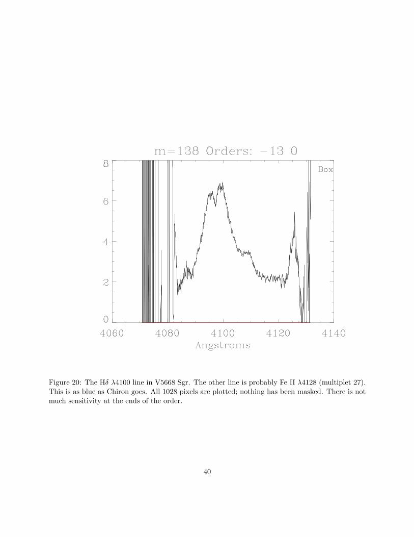
Figure 20: The Hδ λ4100 line in V5668 Sgr. The other line is probably Fe II λ4128 (multiplet 27).This is as blue as Chiron goes. All 1028 pixels are plotted; nothing has been masked. There is notmuch sensitivity at the ends of the order.

40

Figure 21: The Hα region of V745 Sco on 150603. This is the sum of two 1800 second integrations,reduced using ch reduce. The R mag at the time of observation was about 16.2. The dottedred vertical lines mark the spliced regions. No background has been subtracted; the data areunsmoothed. The default trims have been expanded by 10 pixels. The high points are due to lowcounts at the edge of the detector rather than to cosmic rays. The narrow emission is Hα; thesource of the broad emission near 6585A is not currently known. No sky has been subtracted;much of the continuum and the 6563A absorption may be from the night sky.

41

Figure 22: Slicer-mode spectra of nova Sct 2017 on 10 nights between 26 July and 7 August2017, taken during the recommissioning of the spectrograph. Fluxes are normalized to the 6470-6507A continuum. After an initial dip from days 7961 to 7964, the line grew steadily stronger andbroader. The fuzz at 6456 and 6517A is the emerging broad and flat-topped Fe II emission. The6613A absorption is a diffuse interstellar band.

42

While the wavelengths match up well with those of the Yale reductions, I have not tested thefidelity of the solutions. I have not done any rigorous testing of the stability of the wavelengthsolution. Use this code for precise radial velocity work with caution.

Although this code has run on over 1000 images from 572 nights without breaking, there is noguarantee that there are no bugs left, or that all the analysis is being done correctly10. The useralways has the final responsibility for verifying data quality. Bugs or unexpected features may bebrought to the author’s attention at frederick.walter@stonybrook.edu

8 The Software

The procedures and the master calibration files are available in two tar files. Openhttp://www.astro.sunysb.edu/fwalter/SMARTS/NovaAtlas/ch reduce/ch reduce.htmlin your browser. You will find links to this documentation and to ch pros.tar.gz (the procedures)and ch calibs.tar.gz (the master calibrations).

9 Coming Later?

Possible augmentations include:

• Sky subtraction capabilities, using actual spectra of the night sky.

• Testing of optimal extraction codes. At present the Gaussian fit is just that - a Gaussian fit(ignoring data previously flagged as bad). It is possible to flag significant deviations in thedata against the model, and refit excluding those points. If properly tuned, this can removecosmic rays otherwise missed.

10 Summary

This reduction package provides, for both fiber and slicer mode observations, better quality spec-tral extractions for faint targets than those provided by default. Thirteen more orders, from 4085Athrough 4510A, are extracted, and all the points along each spectral order are available. Uncer-tainties (more precisely, the signal-to-noise ratio) are tracked for each point. The extraction doesa better job subtracting the background than does the standard reductions. The extracted spec-tra, when divided by the flats, are flat. This simplifies the problems of flux calibration and ordersplicing.

For slicer mode observations, the 13 bluest orders are also extracted. The interorder backgroundis subtracted globally.

10No process can ever be made completely foolproof, because fools are so ingenious.

43

The output data products are an array of flux-calibrated orders and a single spliced spectrumwith no gaps shortward of 8260A. The data are stored in both fits format and as IDL save files.

This code may enable more kinds of scientifically-useful observations with the Chiron spec-trograph. But it is up to the astronomer to understand their data and the limitations of theinstrument, the data, and the extraction and calibration tools used.

The IDL procedures and the master calibration files are available through my nova web page,http:/www/astro.sunysb.edh/fwalter/SMARTS/NovaAtlas/ .

11 Acknowledgments

I thank the former Provost of Stony Brook University, Dr. Dennis Assanis, for supporting myparticipation in SMARTS. I thank the SMARTS Chiron scheduler, Emily MacPherson, for serviceabove and beyond the call of duty in scheduling Chiron observations of novae in a timely fashion.I thank Andrei Tokovinin for a careful reading of and comments on a draft of this document. Ithank various experts, among them U. Munari, S. Shore, and R. Williams, for looking critically atand questioning some of the spectra I tried to feed them.

Todd Henry challenged me to extend the extractions to the slicer-mode, in return for someengineering data (which looks pretty good scientifically).

Not a penny of NSF money has been expended on this project.

12 References

Markwardt, C. https://www.physics.wisc.edu/∼craigm/idl/fitting.htmlPych, W. 2004, PASP, 116,148Tokovinin, A. et al., 2013, PASP, 125, 1336Valenti, J. 1999. available at https://github.com/mattgiguere/idlutils/blob/master/thid.provan Dokkum, P.G. 2001, PASP 113, 1420

44