Comput Mech (2009) 44:247–261DOI 10.1007/s00466-009-0369-4

ORIGINAL PAPER

An alternative collocation boundary element method for staticand dynamic problems

Thomas Rüberg · Martin Schanz

Received: 11 August 2008 / Accepted: 16 January 2009 / Published online: 11 February 2009© Springer-Verlag 2009

Abstract A collocation boundary element formulation ispresented which is based on a mixed approximation for-mulation similar to the Galerkin boundary element methodpresented by Steinbach (SIAM J Numer Anal 38:401–413,2000) for the solution of Laplace’s equation. The method isalso applicable to vector problems such as elasticity. More-over, dynamic problems of acoustics and elastodynamicsare included. The resulting system matrices have an orderedstructure and small condition numbers in comparison to thestandard collocation approach. Moreover, the employmentof Robin boundary conditions is easily included in this for-mulation. Details on the numerical integration of the occur-ring regular and singular integrals and on the solution of thearising systems of equations are given. Numerical experi-ments have been carried out for different reference problems.In these experiments, the presented approach is comparedto the common nodal collocation method with respect toaccuracy, condition numbers, and stability in the dynamiccase.

Keywords Collocation boundary element method ·Discontinuous elements · Elastodynamics · Robinboundary conditions

T. RübergInstitute for Structural Analysis, Graz University of Technology,Lessingstr. 25, 8010 Graz, Austriae-mail: rueberg@tugraz.at

M. Schanz (B)Institute of Applied Mechanics, Graz University of Technology,Technikerstr. 4, 8010 Graz, Austriae-mail: m.schanz@tugraz.at

1 Introduction

The most prominent boundary element method in structuralengineering remains the nodal collocation method in whichthe approximated boundary integral equation is evaluatedon the interpolation nodes. This method has been applied tonumerous static and dynamic engineering problems [5,6,10].Nodal collocation methods yield system matrices of rathersmall size which are dense, nonsymmetric and often ill-conditioned. In these methods, the dual variable (e.g., sur-face fluxes or tractions) are commonly approximated withthe same continuous polynomials as the primal variable (e.g.,potentials or displacements). But these data have differentmathematical and physical properties [41]. In fact, the dualvariable is not uniquely defined at corners and edges of theconsidered geometry [26] and is thus discontinuous. Seealso [43] for a consideration of the so-called cornerproblem. A common approach to handle these natural discon-tinuities is the introduction of additional data points at cor-ners and edges [26]. Although feasible, this approach requiresthat either the user places these additional nodes or that thecomputer code is capable to do this job automatically. Bothsituations are unsatisfactory and yield a significant amountof additional work.

There are many early works on the use of discontinuouselements for circumventing the problems arising from thediscontinuous nature of the dual variable. For instance, thepublications of Patterson and co-authors [27–29] propose theuse of discontinuous elements for various problems in twoand three spatial dimensions. See also the discussion in [26].Partially discontinuous elements are also proposed in [29]but no algorithm is given which can detect the locations auto-matically where these functions shall be used and where not.Finally, it has to be stated that in all these approaches boththe primal and the dual variable are approximated with the

123

248 Comput Mech (2009) 44:247–261

same type of functions. Therefore, either both are discontinu-ous, partially discontinuous, or continuous. But this conceptignores the fact the primal variable is a (mathematically andphysically) continuous function and, therefore, it seems moresound to treat these fields independently.

Alternatively, the symmetric Galerkin boundary element[41] method has come up which is based on a weightedresidual concept and makes use of two boundary integralequations. The primal and dual variables are approximatedindependently in the correct mathematical subspaces andthe corner problem does therefore not exist anymore. TheseGalerkin schemes yield symmetric positive definite systemmatrices and show a robust performance. Nevertheless, thesecond integral equation is hypersingular and, therefore,needs sophisticated regularization techniques. One approachto treat hypersingular integrals is based on integration byparts. For the case of the Laplace’s equation and the elas-tostatic system, such a regularization is given in [41]. Theregularization of hypersingular kernels for the elastodynam-ic system (as presented below) is given in [16]. Moreover,the computational cost to generate a single matrix entry issignificantly higher than in the collocation method.

In this work, an alternative collocation approach is pre-sented which uses different approximations for primal anddual boundary unknowns. Whereas the former is still approx-imated by continuous functions, the latter is taken to bediscontinuous across the element edges. Therefore, uniquesolutions of the dual variable are facilitated. The collocationpoints are placed strictly inside the elements such that theexpressions for the integral-free term become trivial. The pre-scribed Dirichlet boundary condition will be fulfilled directlyby the approximation and the Neumann boundary conditionis employed by means of a side condition weighted by theshape functions of the primal approximation. With this tech-nique a structured system of equations is obtained whichshows a good conditioning in comparison with the standardcollocation approach. A Galerkin variant of the presented col-location approach has been introduced and mathematicallyanalyzed in [39]. In this reference, the method is presented fora general elliptic partial differential operator and the numeri-cal results refer to Laplace’s equation. Note that the stabilityissues in [39] also appear here and this problem is addressedat the end of Sect. 5. Moreover, Robin boundary conditionsare easily included in this approach and do not require col-umn manipulations of the system matrix or additional sideconditions.

The outline of the paper is to present at first the basicequations in operator notation in Sect. 2. By means of thisabstraction, it is easier to consider scalar and vector problemswith the same notation. The equations are given for static anddynamic problems. Then the spatial and temporal discretiza-tions are presented in Sect. 3, where the convolution quad-rature method is used for the dynamic problems. Afterwards

in Sect. 4, the used numerical integration is explained for theregular and singular surface integrals. A quick description ofthe used direct solution routine follows in Sect. 5. Variousnumerical examples are given with a direct comparison tonodal collocation results and analytical reference solutionsin Sect. 6. Finally Sect. 7 contains a discussion of the advan-tages and disadvantages of the presented method and it closesthe paper. At all crucial points, the differences to the nodalcollocation approach are emphasized.

2 Basic equations

2.1 Boundary value problems

The considered mathematical models in this work are mixedelliptic boundary value problems and hyperbolic initialboundary value problems. On the one hand, Laplace’s equa-tion and the elastostatic system are the elliptic (or static)representatives, see [41], and, on the other hand, the scalarwave equation and the elastodynamic system are the chosenexamples of hyperbolic (or dynamic) Eq. 1. For sake of legi-bility, let L denote an elliptic partial differential operator withconstant coefficients and u is a generic unknown represent-ing, for instance, the acoustic pressure or the displacementfield of an elastic solid. For the models of this work, it holdseither Lu = −κ�u, where κ is the conductivity or compress-ibility of the material and � denotes the Laplace operator,or Lu = −(λ + 2µ)∇ · ∇u + µ∇ × ∇ × u, which is theLamé–Navier [21] operator of elastostatics and λ and µ arethe Lamé constants. Denoting the material density by ρ, theconsidered hyperbolic operators then become

(Hu)(x, t) = ρ ∂2u

∂t2 (x, t)+ (Lu)(x, t). (1)

By means of the above introduced notation, the consideredmixed elliptic boundary value problem is of the form

(Lu)(x) = 0 x ∈ �u�(y) = gD(y) y ∈ �D

q(y) = (T u)(y) = gN (y) y ∈ �N

q(y)+ γ (y)u�(y) = 0 y ∈ �R .

(2)

This problem is stated for the d-dimensional domain� (d =2 or d = 3) with boundary � which is composed of theDirichlet, Neumann, and Robin boundaries,�D, �N , and�R ,respectively. The boundary trace of u is denoted by u� , forwhich the datum gD is prescribed on the Dirichlet boundary�D . The operator T denotes the traction operator or co-nor-mal derivative and maps the unknown u onto the surface fluxor tractions q which are prescribed by gN on the Neumannboundary. Robin boundary conditions combine the boundarydata u� and q by means of the positive function γ (y) on the

123

Comput Mech (2009) 44:247–261 249

Robin boundary �R . For simplicity, body forces or sourceterms are neglected.

In the dynamic case, the mixed initial boundary valueproblem looks like

(Hu)(x, t) = 0 (x, t) ∈ �× It

u�(y, t) = gD(y, t) (y, t) ∈ �D × It

q(y, t) = gN (y, t) (y, t) ∈ �N × It

q(y, t)+ γ (y)u�(y, t) = 0 (y, t) ∈ �R × It ,

(3)

where It is the considered time interval, e.g., It = (0, T )withsome positive time instant T . In addition to Eq. 3, initial con-ditions have to be prescribed for the starting time point. Here,a quiescent past [1] of the material is assumed and, therefore,the initial conditions are identical zero. Hence,

u(x, 0+) = 0 and∂u

∂t(x, 0+) = 0, x ∈ �, (4)

holds, where 0+ denotes the limit t → 0 from above. Notethat for simplicity, the function γ in the Robin boundaryconditions is assumed to be independent of time in the initialboundary value problem (3).

2.2 Boundary integral equations

It is well-known that the solution u of the mixed boundaryvalue problem (2) at any point x inside the domain� is givenby the representation formula [41]

u(x) =∫

�

U (x−y)q(y) dsy−∫

�

(TyU )(x−y)u�(y) dsy (5)

once the boundary data [u�, q] are known for the wholeboundary�. In this expression, U denotes the full-space fun-damental solution of the operator L and TyU is commonlyreferred to as flux or traction kernel. Note that the deriva-tives involved in the application of Ty are with respect to thecoordinate y as indicated by the subscript. Here, the funda-mental solutions for elastostatics, the so-called Kelvin ten-sor [18,21], and for Laplace’s equation [10,41] are employed.

The boundary trace � � x → x ∈ � of Eq. 5 yields thefirst boundary integral equation which reads in operator form

(Cu�)(x)+ (Ku�)(x) = (Vq)(x). (6)

C is the integral-free term and V and K are the single and dou-ble layer operators, respectively, which are defined as [41]

(Vq)(x) =∫

�

U (x − y)q(y) dsy

(Ku�)(x) = limε→0

∫

�\Bε(x)(TyU )(x − y)u�(y) dsy (7)

(Cu�)(x) = u� + limε→0

∫

∂Bε(x)∩�(TyU )(x − y)u�(x) dsy.

In these definitions, Bε(x) is a ball of radius ε centered at xand ∂Bε(x) is its surface.

The mixed boundary value problem (2) can thus be solvedby appropriate use of Eq. 6. A continuous extension gD ofthe given Dirichlet datum is introduced such that

gD(x) = gD(x) x ∈ �D (8)

holds. Moreover, the unknown boundary function u� is nowreplaced by a new unknown

u� = u� − gD, (9)

which is defined on the whole boundary �. By means of theextension (8) and the new unknown (9), the boundary integralEq. 6 becomes

(Vq)(x)−(Cu�)(x)−(Ku�)(x)=(C gD)(x)+(KgD)(x)

(10)

for all x ∈ �. For simplicity, the abbreviations

K = (C +K) and fD = KgD (11)

are introduced, such that Eq. 10 finally reads

(Vq)(x)− (Ku�)(x) = fD(x). (12)

In addition, the Neumann and Robin boundary conditionshave to be employed which require q = gN on �N andq + γ u� = 0 on �R . Adding these conditions to the bound-ary integral Eq. 12, gives the system of operator equations

(V −KI G

)(q

u�

)=

(fD

gN

)(13)

with the identity operator I and the scaling operator G, whichbasically multiplies the function γ with the unknown u� .

In the hyperbolic case, the starting point is now thedynamic representation formula [1],

u�(x, t) =t∫

0

∫

�

U (x − y, t − τ)q(y, τ ) dsy dτ

−t∫

0

∫

�

(TyU )(x − y, t − τ)u�(y, τ ) dsy dτ,

(14)

where U is now the fundamental solution of the hyperbolicoperator H as defined in Eq. 1. Again, the boundary traceyields the first dynamic boundary integral equation

(Ct ∗ u�)(x, t)+ (Kt ∗ u)(x, t) = (Vt ∗ q)(x, t). (15)

123

250 Comput Mech (2009) 44:247–261

In this expression, f ∗ g denotes the temporal convolution,i.e., f ∗g = ∫ t

0 f (t−τ)g(τ ) dτ [42]. The occurring operatorsare now defined as

(Vt ∗ q)(x, t) =t∫

0

∫

�

U (x − y, t − τ)q(y, τ ) dsy dτ

(Kt ∗ u�)(x, t) = limε→0

∫

�\Bε(x)

t∫

0

(TyU )(x − y, t − τ)

×u�(y, τ ) dsy dτ (16)

(Ct ∗ u�)(x, t) = (CIt ∗ u�)(x, t)

= (Cu�)(x, t)

with the same notation as in Eq. 7. In the expression of theintegral-free term, the operator It = Iδ(t) has been usedfor simplicity, which is the identity for the convolution, i.e.,It ∗ f = f . Using again an extension of the prescribedDirichlet datum gD and an auxiliary unknown u� , one arrivesat the equation

(Vt ∗ q)(x, t)− (Kt ∗ u�)(x, t) = fD(x, t), (17)

where abbreviations analogously to Eq. 11 have been made,i.e., Kt = (Ct + Kt ) and fD(x, t) = (Kt ∗ gD)(x, t). TheNeumann boundary conditions are again added as a sidecondition which is facilitated by the identity operator

(It ∗ q)(x, t) = gN (x, t) (18)

and, similarly, the Robin boundary condition is added bymeans of the expression

(It ∗ q)(x, t)+ (Gt ∗ u�)(x, t) = 0. (19)

Here, the operator Gt = Gδ(t) is defined in the same way asthe identity It which is valid since the function γ has beenassumed to be independent of time in the initial boundaryvalue problem (3). The final system of operator equationsthen reads(

Vt −Kt

It Gt

)∗

(q

u�

)=

(fD

gN

). (20)

Classical approach. If the given Neumann datum gN isextended in the same way, i.e., gN (x) = gN (x) on �N ,and a new boundary unknown q is introduced by settingq = q − gN , then Eq. 12 becomes

(V q)(x)− (Ku�)(x) = fD(x)− (V gN )(x). (21)

Comparing Eqs. 12 and 21, it becomes clear that the way,the boundary unknown q is handled, is different. Whereasin Eq. 13 the Neumann boundary condition is used as a sidecondition and, therefore, the whole datum q is treated as anunknown function, in the classical approach (21) the knownand unknown data are well separated. The main differences

become clear when the discretizations are introduced. Theseobservations can be directly transferred to the dynamic case.

3 Discretization

3.1 Spatial discretization

In the sense of a classical finite element discretization, theboundary � is now represented by the computational surface�h which is the union of simple geometric entities, e.g., sur-face triangles or line elements in three or two spatial dimen-sions, respectively. With respect to this surface discretization,shape functions are defined for the spatial approximation ofthe unknown functions u� and q, i.e.,

u�,h(x) =N∑

i=1

ϕi (x)ui and qh(x) =M∑

j=1

ψ j (x)q j . (22)

Note that this approximation has to be altered appropriatelyif u� and q are vector fields, because then Eq. (22) has tobe understood component-wise. Here, the functions ϕi arecontinuous functions as, for instance, the piecewise linearhat functions. The corresponding coefficients ui are then thenodal unknowns of the approximation. On the contrary, theshape functions ψ j are discontinuous and associated withthe elements. Therefore, the coefficients q j refer only to onespecific element and the result can have jumps across theelement boundaries. This choice of shape functions is fairlynatural because, in case of elasticity problems, u� representsthe displacement field of the boundary which has to be con-tinuous according to the assumptions of a continuum. On theother hand, the surface tractions q will have jumps at geom-etry corners and edges and, in addition, the correspondingNeumann datum gN is often applied in form of a discontinu-ous function. Note that this choice is also consistent with therespective trace spaces [39,41] corresponding to the data u�and q in the boundary value problem (2).

The approximations (22) are also used for the givenboundary data, gD and gN , and for the auxiliary unknown u�

gD,h(x) =N∑

i=1

ϕi (x)gD,i

gN ,h(x) =M∑

j=1

ψ j (x)gN , j (23)

u�,h(x) =N∑

i=1

ϕi (x)ui .

Inserting the approximations qh, u�,h , and gD,h into Eq. 12yields a residual. In the sense of collocation techniques, thisresidual is then forced to be zero on a certain set of nodes

123

Comput Mech (2009) 44:247–261 251

{x∗�}L�=1 ⊂ �h , the collocation points. This gives the discret-ized and collocated integral equation

Vq− Ku = fD. (24)

These matrices have the following entries

V[�, j] = (Vψ j )(x∗�) q[ j] = q j

K[�, i] = (Kϕi )(x∗�) u[i] = ui (25)

fD[�] = (KgD,h)(x∗�).

For completeness, the identities q = gN on �N and q +γ u� = 0 on�R have to be added which is done in a weightedsense. This results in the matrix equation

Bq+Gu = fN (26)

with the matrix coefficients

B[k, j] = 〈ϕk, ψ j 〉 fN [k] = 〈ϕk, gN ,h〉(27)

G[k, i] = 〈ϕk, γ ϕi 〉.Here, 〈u, v〉 denotes the L2-product of u and v over theboundary �, i.e., 〈u, v〉 = ∫

�uv ds. The mass matrix B

is thus the discretization of the identity operator I and thematrix G is the discretization of the operator G. Note thatthe vector fN is filled with zeros on the Dirichlet and Robinboundaries, �D and �R , which corresponds to a zero exten-sion of the given datum gN . Combining Eqs. 24 and 26, yieldsthe system of equations(

V −KB G

) (qu

)=

(fD

fN

), (28)

which is of dimension (M + N ) × (L + N ). Obviously,M = L is a necessary condition for the solvability of thissystem which implies that there have to be as many collo-cation equations as coefficients q j . The specific choice ofcollocation points will be discussed below.

In the dynamic case, the situation is very similar. The spa-tial approximation is the same as in Eq. 22, i.e.,

u�,h(x, t) =N∑

i=1

ϕi (x)ui (t)

(29)

qh(x, t) =M∑

j=1

ψ j (x)q j (t),

with the difference that the coefficients ui and q j are stillfunctions of time. Again, the spatial approximation is insertedinto the integral Eq. 16 and the resulting residual is collocatedon the points x∗� . This yields the semi-discrete set of convo-lution equations(

Vt −Kt

Bt Gt

)∗

(qt

ut

)=

(fD,t

fN ,t

). (30)

The matrix entries are now defined by application of thedynamic boundary integral operators to the shape functions

but still ignoring the temporal convolution. Hence, they havethe same form as in Eq. 25, but all the objects are still func-tions of time. Moreover, auxiliary matrix operators Bt and Gt

have been used in order to allow for the condensed notationin Eq. 30 by setting

Bt [k, j]=〈ϕk, ψ j 〉δ(t) and Gt [k, i]=〈ϕk, ϕiγ 〉δ(t). (31)

Obviously, it remains to find a suitable temporal discretiza-tion for the system of Eq. 30.

Note that in the above definitions of matrix entries it hasbeen assumed, for simplicity only, that the application of theboundary integral operators is exact. Of course, these inte-grals will be solved numerically and, therefore, be subjectto errors. The quadrature rules for the evaluation of theseexpressions are discussed in Sect. 4.

Collocation points. As indicated above, one has the neces-sity of using as many collocation equations as coefficients q j .Therefore, it is straightforward to place on every element τe

of the discretization of� as many collocation points as shapefunctions for the unknown q are used on that element. If q is,for instance, approximated by piecewise constant functions,the midpoint of each element seems to be the ideal loca-tion for the collocation points. In case of a piecewise lineardiscontinuous approximation, the situation is more involved.Now, the logical consequence would be to put the colloca-tion points at the vertices of each element. Unfortunately,this makes the collocation equations redundant. Hence, it ispreferred to place them in such a manner that they are dis-tributed uniformly in case of a uniform discretization. Thisimplies that the neighbors of each collocation point are as faraway as possible. It is chosen here, to use the points ξ = ± 1

2from the reference interval −1 ≤ ξ ≤ 1 of linear line ele-ments for a two-dimensional analysis. On the reference tri-angle τ = {0 ≤ ξ1 ≤ 1, 0 ≤ ξ2 ≤ 1− ξ1} for a three-dimen-sional analysis, these points are located at ( 1

6 ,16 ), (

16 ,

23 ), and

( 23 ,

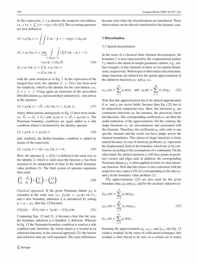
16 ). These positions are depicted in Fig. 1. Note that due

to the fact that the collocation points are strictly inside theelements the surrounding surface is always smooth. There-fore, the integral-free term simply becomes C = 1

2I. Thematrix C which is contained in K has thus the entries

C[�, i] = 1

2ϕi (x∗�). (32)

Obviously, expression (32) is a lot more comfortable as theanalytic expressions for the integral-free term derived in [24]for three-dimensional elastostatics. Moreover, in the expres-sions of [24] material parameters enter. If these are dependenton the Laplace parameter as in the case of the viscoelasticanalysis in [35], they have to be recomputed for every Laplaceparameter.

123

252 Comput Mech (2009) 44:247–261

Fig. 1 Location of the collocation points for a triangle with a con-stant shape function (asterisk) or linear shape functions (bullets) for theapproximation of q

Comparison to nodal collocation. The main difference inthe presented approach to the classical nodal collocation isthe mixed approximation of Eq. 22. In the nodal collocation,one uses exactly the same shape functions for the unknownq as for u� and applies them to the integral Eq. 21. The col-location points are then the nodal coordinates of the spatialdiscretization. The system of equations is then obtained byassembling the columns of the matrices V and K to the leftand right hand sides depending on whether they correspondto an unknown or prescribed coefficient. The application ofthe Robin boundary conditions is then not so straightforwardand requires either additional equations or manipulations ofthe system matrix [13]. The advantages and disadvantages ofthe different approaches are outlined in Sect. 7.

3.2 Temporal discretization

In order to convert system (30) into a series of algebraic equa-tions, the occurring convolution integrals have to be solved.The classical way to do so, is to introduce shape functionsfor the time behavior of the coefficients ui (t) and q j (t) andsolve the resulting integrals analytically [23,34]. Here, theconvolution quadrature method is used, which yields a quad-rature rule for convolution type integrals based on quadratureweights which depend on the Laplace transform of one of theoperands. This method goes back to [22] and has been com-pared with the standard approach in [35]. Whereas the directapproach based on the time-domain fundamental solution Uof the operator H is computationally more efficient, it suf-fers from severe stability restrictions. For this reason andthe possible extension to viscoelastodynamic analyses, the

convolution quadrature method based on the Laplace trans-form fundamental solution U is preferred in this work.

Consider, for simplicity, the application of the spatiallydiscretized single layer operator

h(t) = (Vt ∗ qt )(t) =t∫

0

Vt (t − τ)qt (τ ) dτ. (33)

The value of the resulting vector h at the time instant tn =n�t of an equidistant time grid is now approximated by theformula

h(tn) ≈n∑ν=0

ωn−ν(�t, V, χ)qt (ν�t). (34)

In this approximation, theωn−ν are the weights generated bythe convolution quadrature method and depend on the size ofthe time step, the Laplace transform V of the operator matrixVt , and the characteristic polynomial χ of a suitably chosenmultistep method. Here, a BDF2 [20] is chosen which fulfillsall the criteria of the convolution quadrature method [22].Using now the following notation for n = 0, 1, . . . , andν ≤ n

Vn−ν = ωn−ν(�t, V, χ) qn = qt (n�t)

Kn−ν = ωn−ν(�t, K, χ) un = ut (n�t)fD,n = fD(n�t), fN ,n = fN (n�t)

, (35)

results in the series of systems of equations

(V0 −K0

B G

)(qn

un

)=

(fD,n

fN ,n

)−

n∑ν=1

(Vn−ν Kn−ν

) (qνuν

).

(36)

Note that the matrices B and G are identical with the staticcase and their coefficients are defined in Eq. 27.

4 Numerical integration

In order to obtain the systems of Eqs. 28 and 36, the applica-tion of the respective integral operators has to be carried outnumerically. As common in boundary element methods, onehas to distinguish between the situation when the collocationpoint x∗� is located inside or outside the surface element τe onwhich the integration is carried out. Whereas the former caseof improper integrals needs special attention, the latter caseof a regular integral can be carried out by means of Gaussianquadrature. Nevertheless, the integrand behaves almost sin-gular if the collocation point is close to the region of integra-tion and, therefore, the regular integration also needs specialattention.

123

Comput Mech (2009) 44:247–261 253

4.1 Regular integrals

For sake of simplicity, only the integration on triangles is con-sidered here. Nevertheless, the techniques are easily adaptedfor quadrilateral elements or for the line integrals of a two-dimensional analysis. An exemplary integral is

I (k; x∗) =1∫

0

1−ξ1∫

0

k(x∗, x(ξ1, ξ2)) dξ2 dξ1, (37)

which is obtained after a coordinate transformation from theglobal coordinates to the reference triangle τ . The genericintegrand k contains the shape function, the Gram determi-nant of the coordinate transformation and the fundamentalsolution or its derivative. The latter is assumed to behavelike |x − x∗� |−2 and, therefore, this distance is the crucialmeasure of the quality of the numerical integration. In orderto compute the distance between collocation and integra-tion point in reference coordinates, at first the coordinatesξ∗ = (ξ∗1 , ξ∗2 , ξ∗3 ) such that x(ξ∗) = x∗, have to be computed,where x(ξ) denotes the coordinate transformation from ref-erence to global coordinates. The geometry approximationis assumed to be linear, i.e., x(ξ) = x1 + t1ξ1 + t2ξ2 +nξ3 with the triangle vertices xi (i = 1, 2, 3), the tangentvectors t1 = x2 − x1 and t2 = x3 − x1, and the nor-mal vector n = t1 × t2. Then, the reference coordinatesof the collocation point can be computed by solving theequation

x1 + t1ξ∗1 + tξ∗2 + nξ∗3 = x∗ ⇒ Mξ∗ = x∗ − x1, (38)

where the matrix M is composed of the tangent and normalvectors, M = [t1, t2,n]. In general, the tangent vectors t1 andt2 are not mutually orthogonal. But, by definition, the normalvector n is orthogonal to the plane spanned by the tangentvectors. Therefore, by multiplication with n, the value of ξ∗3is easily computed and Eq. 38 reduces to a 2 × 2-systemwhich is solved easily.

In view of the final criterion for the quality of the quadra-ture, the minimal distance r between the reference triangleτ and the coordinates ξ∗ has to be computed. This is easilydone by detecting the point ξ ∈ τ which lies closest to ξ∗and setting r = |ξ − ξ∗|.

Once these geometrical entities are computed, the errorestimate of [19]

|E p| < C1

2p

1

r p+2 (39)

is used, where C is some constant and p is the maximal orderof a polynomial which is integrated exactly by the quadraturerule. For Gauß–Legendre quadrature in one dimension, onehas the well-known result p = 2ng + 1 with ng denotingthe number of evaluation points the rule is using [17]. Forother quadrature rules, e.g., the triangle rules of [9], which

are used here for a three-dimensional analysis, the order p isusually a given quantity associated with the rule. E p is theerror of that rule of order p and is a prescribed value. Takingthe logarithm of expression (39), yields a rule for the order p

p← 2

⌈log(C)− log |E p| − log(r2)

log(4r2)

⌉(40)

under the assumption that log(4r2) is greater than zero. �x�denotes here the smallest integer greater than or equal to x .

If the order p computed according to the rule (40) is greaterthan some value pmax of the highest quadrature rule avail-able or the condition log(4r2) > 0 is violated, the triangle τis subdivided into four sub-triangles. The numerical integra-tion is then carried out on each of these sub-triangles with anorder pmax unless a further subdivision is necessary. Hence,a recursive scheme is started in which on each sub-trianglethe rule (40) is recomputed with a new value of the minimaldistance r , now with respect to the considered sub-triangle,and a new tolerance which is reduced according to the area ofthe sub-triangle. This recursion takes place until p ≤ pmax

or a maximal level of recursion is reached.Note that Eq. 39 is not understood as a sharp error esti-

mate but rather an expression which grasps the asymptoticbehavior of the integrand. It only refers to the monomial ofr with the highest order and, moreover, it neglects the influ-ence of the shape function and the Gram determinant on theintegrand.

4.2 Singular integration

Here, the collocation point is located inside the element ofintegration, i.e., x∗� ∈ τe. Therefore, the integral kernels ofthe single and double layer operators, V and K (or Vt andKt for the dynamics case), tend to infinity as |y − x∗| → 0.Whereas the integral kernels of the scalar models (Laplace’sequation and scalar wave equation) and the single layer oper-ators of the vector models (elastostatics and elastodynamics)are weakly singular, the double layer operator of the vec-tor models is only defined in the sense of a Cauchy princi-pal value integration [17]. The treatment of such integrals isdescribed in the following Sect. 4.3. For the time being, onlyweakly singular integrals are considered.

A common approach to handle singular integrals in thecontext of boundary element methods, is to subtract the lead-ing singularity which can then be treated by analytical tech-niques or special quadrature rules. The difference term, i.e.,integral kernel minus leading singularity, is thus a regularfunction. Nevertheless, this regularity only refers to the termitself but not to any higher order derivative. But these deriva-tives determine the quadrature error [17]. Consider, forinstance, the Bessel function K0(x) which occurs in the fun-damental solutions of the Laplace transformed scalar wave

123

254 Comput Mech (2009) 44:247–261

equation or elastodynamics. This function has a leadingsingularity of − log(x). The standard approach would be touse a logarithmic quadrature rule [31] for the logarithmicsingularity and then a standard Gaussian quadrature for theterm K0(x) + log(x). But the derivatives of this differenceterm are again singular and, therefore, the quadrature errorcannot be controlled. Due to this observation, it is desirableto have a quadrature rule which is applicable to the integralkernel as a whole.

In the three-dimensional analysis, the weakly singularintegrals over surface triangles are carried out by the rulesdeveloped in [19]. This approach is also known as Duffycoordinates [8] in the mathematical community. The only dif-ference here is that the point of singularity is not located on avertex but inside the element. Therefore, by drawing lines tothe vertices and dropping perpendiculars on the sides, the tri-angle is subdivided into six triangular regions of integrationwhere each one has the singularity on a vertex. Alternatively,one could also use polar coordinates. Confer [10] for a com-parison and [37] for an in-depth mathematical analysis ofthese two approaches.

For the weakly singular line integrals in two-dimensionalanalyses the semi-sigmoidal transformations due to [15] areused. These transformations work in the same black-boxfashion as Duffy coordinates by mapping the region of inte-gration onto itself with a non-linear coordinate transforma-tion which yields a Jacobian alleviating the singularity.

4.3 Regularization

The double layer operator of the elastostatic and elastody-namic equations is only defined in the sense of a Cauchyprincipal value. Therefore, suitable quadrature rules whichcan be used in the desired black-box fashion are not eas-ily constructed. For this reason, it is here preferred to applyan analytical technique which yields a weakly singular rep-resentation. Such techniques are commonly referred to asregularization.

A regularized expression of the elastostatic double layeroperator is given by [18] and has the form (see also [41,25])

(KE u�)(x) = − 1

2(d − 1)π

∫

�

u�(y)(y− x) · n(y)|y− x|d dsy

− 1

2(d − 1)π

∫

�

E(x − y)(Myu�)(y) dsy

+ 2µ(V E (Myu�))(x). (41)

Recall that d = 2, 3 is the dimension of the problem and nthe unit outward normal vector. The function E(x) is eitherE(x) = − log |x| or E(x) = 1/|x| for the cases d = 2 or

d = 3, respectively. The operator My appearing in Eq. 41 isreferred to as Günther derivative [18] and has the components

My[i, j] = n j (y)∂

∂yi− ni (y)

∂

∂y j, (42)

where yi is the i th component direction of the position vec-tor y and ni is the i th component of the normal vector n(y)located at the boundary point y. A derivation and alternativerepresentations of Eq. 42 are given in [41]. Expression (41)is composed of three parts, the double layer operator ofLaplace’s equation and the single layer operators of Laplace’sequation and Elastostatics. The latter two are not applied tothe function u� itself but to special derivatives of it with theoperation due to Eq. 42. All three integral operators are nowweakly singular and the application of My is well definedbecause the test functions used for the approximation of u� ,see Eq. 22, are continuous.

In the remaining case of elastodynamics, an expressionsimilar to Eq. 41 can be derived and is given in [16] for thethree-dimensional case. The transfer to two dimensions isstraightforward and not repeated here. Note that in the der-ivation of these regularizations, the boundary � is assumedto be a closed surface such that ∂� = ∅ holds, i.e., the sur-face itself has no boundary. For some applications, e.g., thediscretization of an elastic halfspace by a surface patch, thisassumption is violated.

5 Solution of the systems

Due to the spatial and temporal discretizations as presented inSects. 3.1 and 3.2, the systems of Eqs. 28 and 36 are obtained.The block matrix of both systems has exactly the same struc-ture. But in the dynamic case, system (36) has to be solvedrepeatedly for different right hand sides. Therefore, a directsolver can be still advantageous and is considered here. Forsimplicity, only system (28) is considered in the following.

A static condensation of the system of Eq. 28 gives thereduced system of equations

Su = g, (43)

where S = G + BV−1K and g = fN − BV−1fD . UsingLU-factorizations [11] instead of computing the inverse ofV, yields the following steps

LV UV = V, LV UK = KLBUV = B, S = G+ LBUK ,

(44)

which are one LU-factorization, two forward-backward sub-stitutions, and one matrix-matrix multiplication. The righthand side g is computed by similar operations. The solutionof system (43) is then another LU-solve. Once the coefficientsu are known, the vector q is easily computed. The solution

123

Comput Mech (2009) 44:247–261 255

steps (44) can be carried out by any linear algebra package,e.g., [2]. It has to be noted that the use of pivotization might benecessary and, therefore, these steps need additional columnand row interchanges which are not outlined here.

Stability problem. Assume now that G = 0, i.e., that noRobin boundary conditions are prescribed because this sit-uation corresponds to the worst case scenario. As outlinedin [39], the type of approximation used in Eq. 22 is crucialfor the stable solution of system (28). The basic conditionsfor the invertibility of the considered system are the existenceof the inverses V−1 and S−1 [4]. Whereas the existence ofV−1 is assumed based on the theoretical knowledge that V isan elliptic operator and the experience that collocation meth-ods in combination with conforming discretizations work.The existence of S−1 is rather tricky and two necessary con-ditions are considered.

At first M > N is postulated, i.e., there have to be morecoefficients q j than ui . The other condition is that the matri-ces K and B have full rank, i.e., rank(K) = rank(B) = N .Both conditions can be fulfilled by either choosing a finermesh for the approximation of q or by using equal orderapproximations [39]. The latter option is considered hereand implies that, for instance, piecewise linear continuoustrial functions are used for u�,h and piecewise linear discon-tinuous functions for qh . Unfortunately, the rank conditionrules out the use of piecewise constant shape functions forqh which would be a natural choice with less degrees offreedom.

6 Numerical results

6.1 Bar problem

Consider the one-dimensional problem depicted in Fig. 2,where a bar of length � is fixed at its left end and loaded at itsright end. In terms of an elastic model, the displacement fieldis prescribed with zero at x1 = 0 and the surface traction isgiven as q = F at x1 = �. In dynamics, the applied forceterm F is assumed to behave like F(t) = F0 H(t) in timewith H(t) denoting the Heaviside or unit step function.

The physical interpretations of this problem are either acolumn of an acoustic fluid subject to a specific surface fluxor the already mentioned elastic bar with an applied trac-tion. In the former case, the material parameters are assumedas κ = 1.42 · 105 N/m2 and ρ = 1.2 kg/m3 for the com-

Fig. 2 Bar subject to axial force

(a) (b) (c)

Fig. 3 Different spatial discretizations: a h = 0.5 m; b h = 0.25 m;c h = 0.2 m

pressibility modulus and the mass density of the acousticfluid, respectively. The elastic solid has the Lamé parametersλ = 0 and µ = 1.06 · 1011 N/m2 and a mass density ofρ = 7 850 kg/m3.

A three-dimensional cuboid of dimension 3× 1× 1 m isused for the representation of this problem which is discret-ized by surface triangles of three different sizes. The shorterside lengths of these triangles are taken as h = 0.5, 0.25, and0.2 m which yields 112, 448, and 700 triangles, respectively.The different meshes are depicted in Fig. 3.

The temporal discretization is carried out as described inSect. 3.2. The size of the time steps�t are then chosen suchthat the CFL-number [7]

β = c1�t

h(45)

has specific values, where c1 denotes the velocity of the com-pression wave. For the acoustic fluid it becomes c2

1 = κ/ρand c2

1 = (λ+ 2µ)/ρ for the elastic solid.

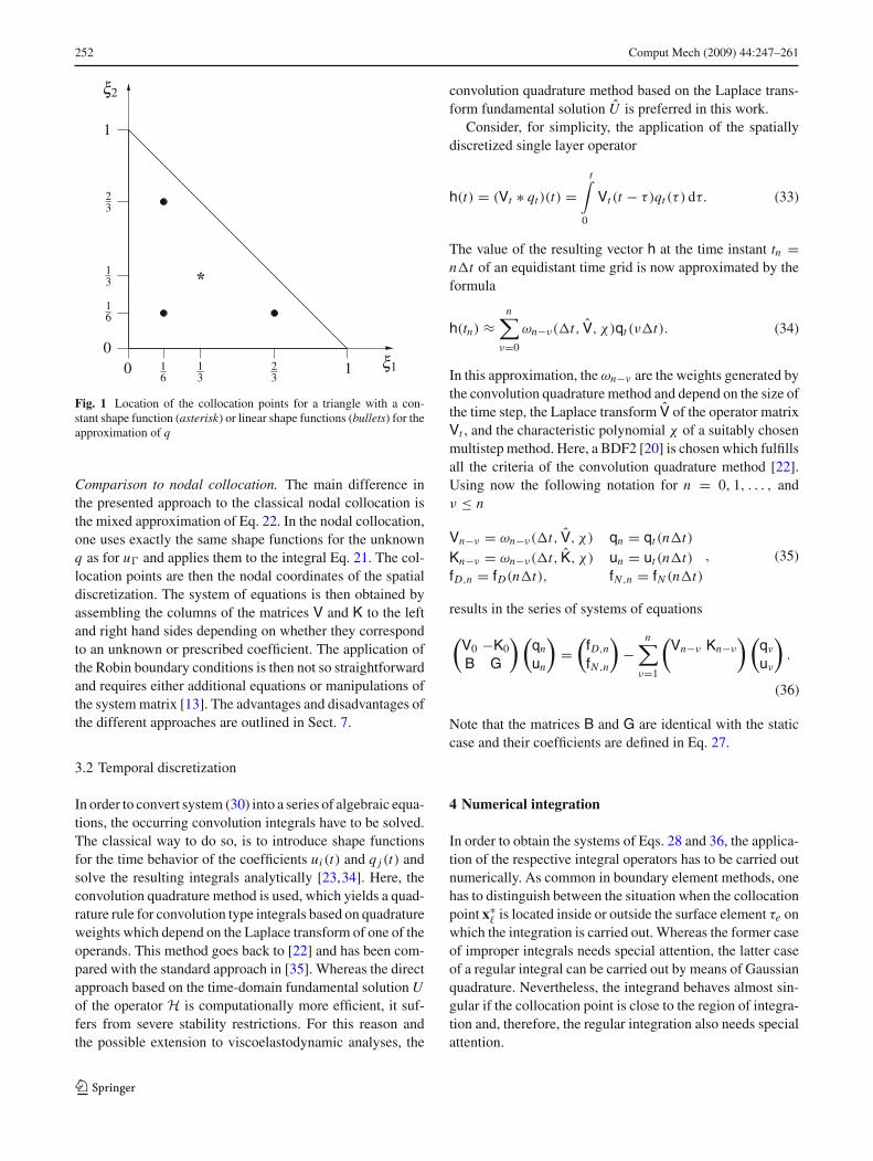
Condition numbers. In the following, the condition numbersof the system matrices for the proposed method are com-pared with the condition numbers of the nodal collocation.The condition number cond(A) is measured in the one-norm,i.e., cond(A) = ‖A‖1‖A−1‖1. In fact, the condition numberestimate of LAPACK [2] is used which is based on the algo-rithm of [14]. Let A be the system matrix obtained by nodalcollocation. V denotes the upper left block matrix of sys-tem (28) or (36) for the static or the dynamics case, respec-tively. Furthermore, S is the Schur complement obtained bystatic condensation as given in Eq. 43. The dimensions ofthese matrices are given in Table 1 for the three differentmeshes and the two considered materials.

In Table 2, the respective condition numbers for theLaplace equation (fluid) and elastostatics (solid) are given forthe three different meshes. It has to be noted that the matrixA is assembled after a variable transformation in which thegeometry and the material parameters are scaled to achieve abetter condition number (see [36] for details on this scaling).Without this variable transformation, the number cond(A)would be totally out of bound. Comparing the numbers ofTable 2, it becomes clear that the condition numbers of A,V,and S are of comparable magnitudes for Laplace equation.

123

256 Comput Mech (2009) 44:247–261

Table 1 Dimensions of the system matrices for different meshes

Mesh dim(A) dim(V) dim(S)

Fluid a 58 336 49

b 226 1,344 201

c 352 2,100 316

Solid a 174 1,008 147

b 678 4,032 603

c 1,056 6,300 948

Table 2 Condition numbers for the static computations

Mesh cond(A) cond(V) cond(S)

Fluid a 215 137 132

b 352 277 240

c 716 344 343

Solid a 4,100 207 5,761

b 7,740 420 11,695

c 8,048 550 16,180

But in the case of elastostatics, V is still well-conditioned,whereas the matrices A and S have condition numbers aboutone order of magnitude greater with cond(A) < cond(S).

In Table 3, the condition number for the dynamic cases aregiven, where the three meshes with three different time stepsizes are compared. The time steps are such that the CFL-number has the values β = 0.2, β = 0.4, and β = 0.8. Theresults for the scalar wave equation are shown in Table 3a andthe Table 3b gives the values for the elastodynamics system.

In the dynamic case, the condition numbers cond(A) aresignificantly larger than cond(V) and cond(S). Moreover,the asymptotic behavior of these condition numbers differsfor the compared methods. The number cond(A) gets largerwith more degrees of freedom and smaller for increasingtime steps. On the contrary, the condition number of the sin-gle layer matrix cond(V) becomes smaller for finer meshes

and larger for bigger time steps. The behavior of cond(S),the condition number of the Schur complement, is not soeasily described. In most cases, it becomes slightly biggerwith an increase of degrees of freedom. But if the time stepis increased, it gets smaller in the fluid case and larger in thesolid case.

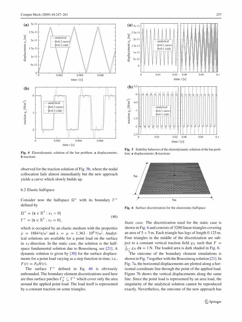
Accuracy and stability. The considered one-dimensionalproblem has an analytical solution which is derived in [12],see also [34]. In order to compare the quality of the numer-ical results, this analytical solution is used as a reference.The outcome of an elastodynamic solution of the consideredproblem is shown in Fig. 4, where the longitudinal displace-ment component u1 is considered at the right end x1 = � inFig. 4a and the surface traction q1 at the left end x1 = 0 inFig. 4b. The computation has been carried out for the coars-est mesh with h = 0.5 m only and a time step size such thatβ = 0.2. In the figures, old refers to nodal collocation andnew to the here proposed method without being judgemental.

Comparing the displacement results of the different col-location approaches in Fig. 4a, one can see that the proposedmethod has less damping of the amplitudes. Moreover, theinitial elongation is already slightly closer to the analyticalcurve. In view of the traction results in Fig. 4b, the outcomeof the new approach gets closer to the jumps of the piecewiseconstant analytical solution. This in turn justifies the largerovershoots after these jumps.

Finally, the behavior of the two compared approaches isconsidered for a smaller time step such that β = 0.1. Theresults are shown together with the analytical solution inFig. 5. In order to emphasize the different stability behav-iors, the time range 0.2 s < t < 0.8 s is not plotted. Onlythe beginning and the end of the computed time period aredisplayed. Clearly, the displacement solution given in Fig. 5agets out of bound after only a short time period for the nodalcollocation, whereas the outcome of the proposed approachremains stable and close to the analytical curve for a signifi-cantly larger simulation time. The same phenomenon can be

Table 3 Condition numbers forthe dynamic computations (a) Fluid

Mesh a a a b b b c c c

β 0.2 0.4 0.8 0.2 0.4 0.8 0.2 0.4 0.8

cond(A) 75.1 51.1 46.4 153 101 86.0 625 413 351

cond(V) 7.49 14.7 28.3 7.71 13.1 25.9 4.33 7.98 16.7

cond(S) 8.43 7.06 5.89 8.74 7.23 5.46 9.08 8.90 8.25

(b) Solid

cond(A) 267 187 181 540 353 311 705 463 417

cond(V) 9.32 15.2 30.9 9.19 16.1 28.4 5.66 9.50 16.8

cond(S) 13.1 14.8 17.4 12.0 14.3 15.9 13.8 15.4 23.6

123

Comput Mech (2009) 44:247–261 257

0 0.002 0.004 0.0060

5e-12

1e-11

1.5e-11

2e-11

2.5e-11

3e-11(a)

(b)

disp

lace

men

tu1 [

m]

analyticalβ=0.2 (new)β=0.2 (old)

time t [s]

0 0.002 0.004 0.006

-2

-1

0

trac

tion

q 1 [N

/m2 ]

analyticalβ=0.2 (new)β=0.2 (old)

time t [s]

Fig. 4 Elastodynamic solution of the bar problem: a displacements;b tractions

observed for the traction solution of Fig. 5b, where the nodalcollocation fails almost immediately but the new approachyields a curve which slowly builds up.

6.2 Elastic halfspace

Consider now the halfspace �+ with its boundary �+defined by

�+ = {x ∈ R3 : x3 > 0}

(46)�+ = {x ∈ R

3 : x3 = 0},which is occupied by an elastic medium with the propertiesρ = 1884 kg/m3 and λ = µ = 1.363 · 108 N/m2. Analyt-ical solutions are available for a point load on the surfacein x3-direction. In the static case, the solution is the half-space fundamental solution due to Boussinesq, see [21]. Adynamic solution is given by [30] for the surface displace-ments for a point load varying as a step function in time, i.e.,F(t) = F0 H(t).

The surface �+ defined in Eq. 46 is obviouslyunbounded. The boundary element discretizations used hereare thus surface patches �+h � �+ which cover only the areaaround the applied point load. The load itself is representedby a constant traction on some triangles.

0

5e-12

1e-11

1.5e-11

2e-11

2.5e-11

3e-11(a)

disp

lace

men

tu1 [

m]

analyticalβ=0.1 (new)β=0.1 (old)

0 0.01 0.02 0.08 0.09 0.1

time t [s]

time t [s]

-2.5

-2

-1.5

-1

-0.5

0

0.5

trac

tion

q 1 [N

/m2 ]

analyticalβ=0.1 (new)β=0.1 (old)

0 0.01 0.02 0.08 0.09 0.1

(b)

Fig. 5 Stability behavior of the elastodynamic solution of the bar prob-lem: a displacements; b tractions

5m

5m

Fig. 6 Surface discretization for the elastostatic halfspace

Static case. The discretization used for the static case isshown in Fig. 6 and consists of 3200 linear triangles coveringan area of 5× 5 m. Each triangle has legs of length 0.125 m.Four triangles in the middle of the discretization are sub-ject to a constant vertical traction field gN such that F =∫�+h

gN dx = 1 N. The loaded area is dark shaded in Fig. 6.The outcome of the boundary element simulations is

shown in Fig. 7 together with the Boussinesq solution [21]. InFig. 7a, the horizontal displacements are plotted along a hor-izontal coordinate line through the point of the applied load.Figure 7b shows the vertical displacements along the sameline. Since the point load is represented by an area load, thesingularity of the analytical solution cannot be reproducedexactly. Nevertheless, the outcome of the new approach has

123

258 Comput Mech (2009) 44:247–261

-2 -1 0 1 2position x1 [m]

position x1 [m]

-2e-09

-1e-09

0

(a)

1e-09

2e-09

disp

lace

men

tu1 [

m]

Boussinesqnewold

-2 -1 0 1 20

5e-09

1e-08

1.5e-08

2e-08

disp

lace

men

tu3 [

m]

Boussinesqnewold

(b)

Fig. 7 Analytical and computed solution of the elastostatic halfspace:a horizontal displacements; b vertical displacements

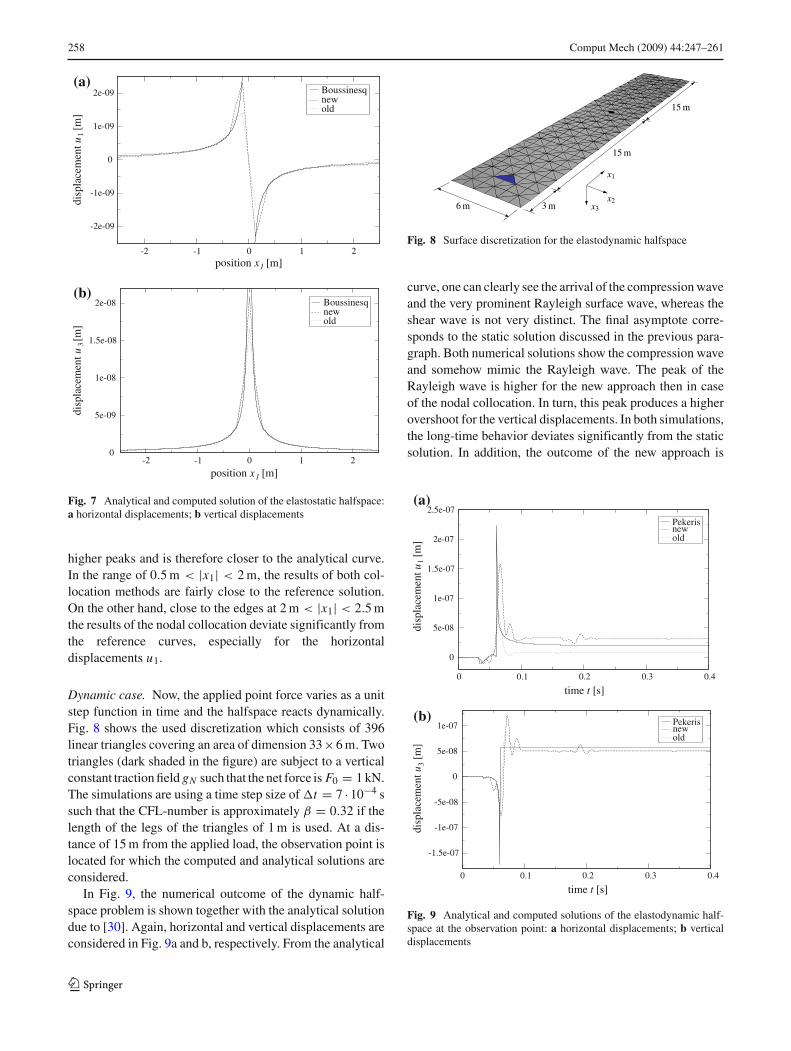
higher peaks and is therefore closer to the analytical curve.In the range of 0.5 m < |x1| < 2 m, the results of both col-location methods are fairly close to the reference solution.On the other hand, close to the edges at 2 m < |x1| < 2.5 mthe results of the nodal collocation deviate significantly fromthe reference curves, especially for the horizontaldisplacements u1.

Dynamic case. Now, the applied point force varies as a unitstep function in time and the halfspace reacts dynamically.Fig. 8 shows the used discretization which consists of 396linear triangles covering an area of dimension 33×6 m. Twotriangles (dark shaded in the figure) are subject to a verticalconstant traction field gN such that the net force is F0 = 1 kN.The simulations are using a time step size of�t = 7 · 10−4 ssuch that the CFL-number is approximately β = 0.32 if thelength of the legs of the triangles of 1 m is used. At a dis-tance of 15 m from the applied load, the observation point islocated for which the computed and analytical solutions areconsidered.

In Fig. 9, the numerical outcome of the dynamic half-space problem is shown together with the analytical solutiondue to [30]. Again, horizontal and vertical displacements areconsidered in Fig. 9a and b, respectively. From the analytical

6 m 3 m

15 m

15 m

x3x2

x1

Fig. 8 Surface discretization for the elastodynamic halfspace

curve, one can clearly see the arrival of the compression waveand the very prominent Rayleigh surface wave, whereas theshear wave is not very distinct. The final asymptote corre-sponds to the static solution discussed in the previous para-graph. Both numerical solutions show the compression waveand somehow mimic the Rayleigh wave. The peak of theRayleigh wave is higher for the new approach then in caseof the nodal collocation. In turn, this peak produces a higherovershoot for the vertical displacements. In both simulations,the long-time behavior deviates significantly from the staticsolution. In addition, the outcome of the new approach is

0 0.1 0.2 0.3 0.4

time t [s]

0 0.1 0.2 0.3 0.4

time t [s]

0

5e-08

1e-07

1.5e-07

2e-07

2.5e-07(a)

disp

lace

men

tu1 [

m]

Pekerisnewold

-1.5e-07

-1e-07

-5e-08

0

5e-08

1e-07

disp

lace

men

tu3

[m]

Pekerisnewold

(b)

Fig. 9 Analytical and computed solutions of the elastodynamic half-space at the observation point: a horizontal displacements; b verticaldisplacements

123

Comput Mech (2009) 44:247–261 259

F

EIx

k

�/2 �/2

Fig. 10 Continuously bedded beam

polluted by artificial wave reflections. These reflections alsooccur in the compared nodal collocation but less severely. Itcan be assumed that these strong reflections are caused by theregularization of the double layer operator, given in Eq. 41.This expression is based on the assumption that the bound-ary � is a closed surface which is violated in the consideredcase of the halfspace. Nevertheless, the computed solutionremains stable and the magnitudes of these wave reflectionsdiminish.

6.3 Beam on elastic foundation

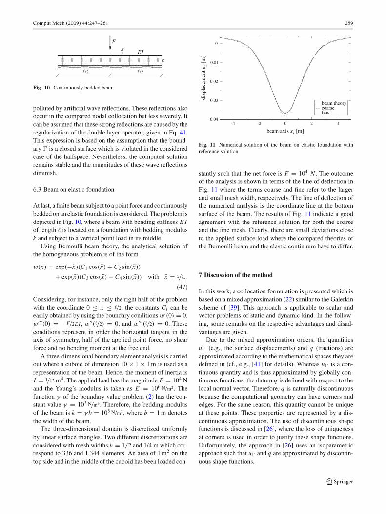
At last, a finite beam subject to a point force and continuouslybedded on an elastic foundation is considered. The problem isdepicted in Fig. 10, where a beam with bending stiffness E Iof length � is located on a foundation with bedding modulusk and subject to a vertical point load in its middle.

Using Bernoulli beam theory, the analytical solution ofthe homogeneous problem is of the form

w(x) = exp(−x)(C1 cos(x)+ C2 sin(x))

+ exp(x)(C3 cos(x)+ C4 sin(x)) with x = x/λ.

(47)

Considering, for instance, only the right half of the problemwith the coordinate 0 ≤ x ≤ �/2, the constants Ci can beeasily obtained by using the boundary conditionsw′(0) = 0,w′′′(0) = −F/2E I , w′′(�/2) = 0, and w′′′(�/2) = 0. Theseconditions represent in order the horizontal tangent in theaxis of symmetry, half of the applied point force, no shearforce and no bending moment at the free end.

A three-dimensional boundary element analysis is carriedout where a cuboid of dimension 10 × 1 × 1 m is used as arepresentation of the beam. Hence, the moment of inertia isI = 1/12 m4. The applied load has the magnitude F = 104 Nand the Young’s modulus is taken as E = 106 N/m2. Thefunction γ of the boundary value problem (2) has the con-stant value γ = 105 N/m3. Therefore, the bedding modulusof the beam is k = γ b = 105 N/m2, where b = 1 m denotesthe width of the beam.

The three-dimensional domain is discretized uniformlyby linear surface triangles. Two different discretizations areconsidered with mesh widths h = 1/2 and 1/4 m which cor-respond to 336 and 1,344 elements. An area of 1 m2 on thetop side and in the middle of the cuboid has been loaded con-

-4 -2 0 2 4

beam axis x1 [m]

0

0.01

0.02

0.03

0.04

disp

lace

men

tu3

[m]

beam theorycoarsefine

Fig. 11 Numerical solution of the beam on elastic foundation withreference solution

stantly such that the net force is F = 104 N . The outcomeof the analysis is shown in terms of the line of deflection inFig. 11 where the terms coarse and fine refer to the largerand small mesh width, respectively. The line of deflection ofthe numerical analysis is the coordinate line at the bottomsurface of the beam. The results of Fig. 11 indicate a goodagreement with the reference solution for both the coarseand the fine mesh. Clearly, there are small deviations closeto the applied surface load where the compared theories ofthe Bernoulli beam and the elastic continuum have to differ.

7 Discussion of the method

In this work, a collocation formulation is presented which isbased on a mixed approximation (22) similar to the Galerkinscheme of [39]. This approach is applicable to scalar andvector problems of static and dynamic kind. In the follow-ing, some remarks on the respective advantages and disad-vantages are given.

Due to the mixed approximation orders, the quantitiesu� (e.g., the surface displacements) and q (tractions) areapproximated according to the mathematical spaces they aredefined in (cf., e.g., [41] for details). Whereas u� is a con-tinuous quantity and is thus approximated by globally con-tinuous functions, the datum q is defined with respect to thelocal normal vector. Therefore, q is naturally discontinuousbecause the computational geometry can have corners andedges. For the same reason, this quantity cannot be uniqueat these points. These properties are represented by a dis-continuous approximation. The use of discontinuous shapefunctions is discussed in [26], where the loss of uniquenessat corners is used in order to justify these shape functions.Unfortunately, the approach in [26] uses an isoparametricapproach such that u� and q are approximated by discontin-uous shape functions.

123

260 Comput Mech (2009) 44:247–261

This new collocation scheme is tailored to yield a squarematrix V as the discretization of the single layer operator V .Since V is generally known to be elliptic [41], its discreti-zation with Galerkin schemes results in symmetric positivedefinite system matrices. The presented collocation destroysthis symmetry but numerical experiments affirm that V is stillpositive definite. In view of iterative solution algorithms thisproperty might be useful. Nevertheless, it guarantees that Vis invertible. Moreover, the condition numbers of this matrixare very small and seem to be of order O(h−1) as it canbe deduced from the analysis in Sect. 6.1. The collocationpoints are always placed strictly inside the elements suchthat the surrounding surface is smooth. This has the advan-tage that the integral-free term C reduces to C = 1

2I whichis significantly easier to compute than in the nodal colloca-tion (see [24] for the expressions of C for three-dimensionalelastostatics).

The final system of Eq. 28 [or (36) for dynamic problems]is obtained by introducing the Neumann boundary conditionsin a weighted sense by using the mass matrix B. Moreover,Robin boundary conditions are easily implemented by usinganother mass matrix G. This system is well structured incontrast to the nodal collocation approach where the systemmatrix is usually a mixture of columns of V and K. Thismixture is often ill-conditioned and needs dimension-lessvariables to obtain reasonably small condition numbers. Thecondition numbers cond(A) given in Sect. 6.1 are based onsuch variable transformations. Nevertheless, the conditionnumbers due to the proposed method are (with the exceptionof elastostatics) smaller than in the nodal collocation despitetheir larger sizes. This is especially the case in the dynamicanalyses.

The Schur complement of systems (28) and (36) resemblesa Dirichlet-to-Neumann map [38]. It has mapping propertiessimilar to a finite element stiffness matrix and, therefore, iswell-suited for the coupling of boundary with finite elementmethods. Such a coupling scheme, which is independent ofthe discretization method on the subdomain level, has beenproposed in [33] based on the presented collocation method.

The new approach is based on the globally discontinu-ous approximation of q in Eq. 22 and treats every coefficientq j of the approximation as an unknown quantity. For thisreason the system matrices are significantly larger than in thenodal collocation. Consider for instance, the case of three-dimensional elasticity with a piecewise linear discontinuousapproximation of the tractions. In that case, every surfaceelement τe has nine unknown traction coefficients and thedimension of the system matrix V is thus (9Ne)

2, where Ne

denotes the number of elements. The presented formulationallows for the use of a piecewise constant traction approxi-mation but, unfortunately, the combination of linear and con-stant shape functions spoils the solvability of the final systemof equations [39]. Possibly, stabilization techniques known

from mixed finite element methods [4] could be adapted tothe system of this collocation approach such that the use ofconstant shape functions for the approximation of the dualvariable q becomes feasible.

In any case, it can be assumed that matrix approximationtechniques such as the adaptive cross approximation [3] (seealso [32]) would yield good approximation rates if appliedto the matrix V. Moreover, the use of iterative solution meth-ods tailored to systems of the type (28) could significantlyspeed up the solution procedure because of the good con-dition numbers of the block matrices V and S. Such pre-conditioned iterative solvers are so far only available for thesymmetric Galerkin method [40].

Another drawback of the proposed approach is the place-ment of the collocation points which is so far heuristic. Itwould be desirable to have a criterion at hand which is basedon mathematical analysis.

8 Conclusion

A novel collocation approach has been presented with valu-able properties. It combines the natural approximation spaceswith a structured and well conditioned system matrix. More-over, the inclusion of Robin boundary conditions is straight-forward. But these features come with a high-numerical costsuch that the method in its current state can only be appliedto rather small-sized problems. Nevertheless, this problemcould be reduced. The use of iterative solvers with matrixcompression techniques would significantly speed up thesolution process and reduce the storage requirements.

References

1. Achenbach JD (2005) Wave propagation in elastic solids.North-Holland, Amsterdam

2. Anderson E, Bai Z, Bischof C, Blackford S, Demmel J, Don-garra J, Du Croz J, Greenbaum A, Hammarling S, McKenney A,Sorensen D (1999) LAPACK Users’ Guide. Society for Industrialand Applied Mathematics, 3rd edn

3. Bebendorf M, Rjasanow S (2003) Adaptive low-rank approxima-tion of collocation matrices. Computing 70:1–24

4. Benzi M, Golub GH, Liesen J (2005) Numerical solution of saddlepoint problems. Acta Numer 14:1–137

5. Beskos DE (1987) Boundary element methods in dynamicsanalysis. Appl Mech Rev 40:1–23

6. Beskos DE (1997) Boundary element methods in dynamic analy-sis: part II (1986–1996). Appl Mech Rev 50(3):149–197

7. Courant R, Friedrichs K, Lewy H (1928) Über die partiellen Differ-enzengleichungen der mathematischen Physik. Math Ann 100:32–74

8. Duffy MG (1982) Quadrature over a pyramid or cube of inte-grands with a singularity at a vertex. SIAM J Numer Anal 19:1260–1262

123

Comput Mech (2009) 44:247–261 261

9. Dunavant DA (1985) High degree efficient symmetrical Gaus-sian quadrature rules for the triangle. Int J Numer Methods Eng21:1129–1148

10. Gaul L, Kögl M, Wagner M (2003) Boundary element methods forengineers and scientists. Springer, Heidelberg

11. Golub GH, van Loan CF (1996) Matrix computations. Johns Hop-kins University Press, Baltimore

12. Graff KF (1991) Wave motions in elastic solids. Dover, New York13. Hartmann F (1989) Introduction to boundary elements. Theory and

applications. Springer, Heidelberg14. Higham NJ (1988) FORTRAN codes for estimating the one-norm

of a real or complex matrix, with applications to condition estima-tion. ACM Trans Math Softw 14:381–396

15. Johnston PR (2000) Semi-sigmoidal transformations for evaluat-ing weakly singular boundary element integrals. Int J NumerMethods Eng 47:1709–1730

16. Kielhorn L, Schanz M (2007) CQM based symmetric GalerkinBEM: regularization of strong and hypersingular kernels in 3-delastodynamics. Int J Numer Methods Eng. doi: 10.1002/nme.2381

17. Krommer AR, Ueberhuber CW (1998) Computational integration.SIAM

18. Kupradze VD, Gegelia TG, Basheleishvili MO, Burchuladze TV(1979) Three-dimensional problems of the mathematical theory ofelasticity and thermoelasticity. North-Holland, Amsterdam

19. Lachat JC, Watson JO (1976) Effective numerical treatment ofboundary integral equations: a formulation for three-dimensionalelastostatics. Int J Numer Methods Eng 10:991–1005

20. Lambert JD (1990) Numerical methods for ordinary differentialsystems. Wiley, New York

21. Love AEH (1944) Treatise on the mathematical theory of elasticity.Dover, New York

22. Lubich C (1988) Convolution quadrature and discretized opera-tional calculus I & II. Numer Math 52:129–145; 413–425

23. Mansur WJ (1983) A time-stepping technique to solve wave prop-agation problems using the boundary element method. PhD thesis,University of Southampton

24. Mantic V (1993) A new formula for the c-matrix in the Somiglianaidentity. J Elast 33:193–201

25. Of G (2006) BETI-Gebietszerlegungsmethoden mit schnellenRandelementverfahren und Anwendungen. PhD thesis, Universityof Stuttgart

26. París F, Cañas J (1997) Boundary element method. OxfordUniversity Press, Oxford

27. Patterson C, Elsebai NAS (1982) A regular boundary methodusing non-conforming elements for potentials in three dimensions.In: Brebbia CA (ed) Boundary element methods in engineering,pp 112–126

28. Patterson C, Sheikh MA (1981) Non-conforming boundary ele-ments for stress analysis. In: Brebbia CA (ed) Boundary elementmethods, pp 137–152

29. Patterson C, Sheikh MA (1984) Interelement continuity in theboundary element method. In: Brebbia CA (ed) Topics in boundaryelement research. Springer, Heidelberg, pp 121–141

30. Pekeris CL (1955) The seismic surface pulse. Proc Natl Am Soc41:469–480

31. Press WH, Teukolsky SA, Vetterling WT, Flannery BP (2002)Numerical Recipes in C++. Cambridge University Press,Cambridge

32. Rjasanow S, Steinbach O (2007) The fast solution of boundaryintegral equations. Springer, Heidelberg

33. Rüberg T (2008) Non-conforming FEM/BEM coupling in timedomain, volume 3 of computation in engineering and science. Ver-lag der Technischen Universität Graz

34. Schanz M (2001) Wave propagation in viscoelastic and poroelasticcontinua—A boundary element approach. Springer, Heidelberg

35. Schanz M, Antes H (1997) A new visco- and elastodynamic timedomain boundary element formulation. Comput Mech 20:452–459

36. Schanz M, Kielhorn L (2005) Dimensionless variables in a Poroelastodynamic time domain bounday element formulation. BuildRes J 53(2–3):175–189

37. Schwab C, Wendland WL (1992) On numerical cubature of singu-lar surface integrals in boundary element methods. Numer Math62:343–369

38. Steinbach O (2003) Stability estimates for hybrid domaindecomposition methods. Springer, Heidelberg

39. Steinbach O (2000) Mixed approximations for boundary elements.SIAM J Numer Anal 38:401–413

40. Steinbach O (1998) Fast solution techniques for the symmetricboundary element method in linear elasticity. Comput MethodsAppl Mech Eng 157:185–191

41. Steinbach O (2008) Numerical approximation methods for ellipticboundary value problems. Springer, Heidelberg

42. Wheeler LT, Sternberg E (1968) Some theorems in classicalelastodynamics. Arch Ration Mech Anal 31:51–90

43. Yan G, Lin F-B (1994) Treatment of corner node problems and itssingularity. Eng Anal Bound Elem 13:75–81

123