NASA-CR-202109

Reprinted from JOURNAL OF CLIMATE, Vo]. 8, No. 5, May 1995

American Meteorological Society //

An Algorithm to Generate Deep-Layer Temperatures from Microwave Satellite

Observations for the Purpose of Monitoring Climate Change

MITCHELL D. GOLDBERG AND HENRY E. FLEMING*

NOAA /National Environmental Satellite. Data. attd hr[brrnation S(,twice. Satellite Research Lahoratoo,, Washington. D("

(Manuscript received 31 January 1994, in final form 6 September 1994)

ABSTRACT

An algorithm for generating deep-layer mean temperatures from satellite-observed microwave observationsis presented. Unlike traditional temperature retrieval methods, this algorithm does not require a first guesstemperature of the ambient atmosphere. By eliminating the first guess a potentially systematic source of errorhas been removed. The algorithm is expected to yield long-term records that are suitable for detecting smallchanges in climate.

The atmospheric contribution to the deep-layer mean temperature is given by the averaging kernel. Thealgorithm computes the coefficients that will best approximate a desired averaging kernel from a linear combinationof the satellite radiometer's weighting functions. The coefficients are then applied to the measurements to yieldthe deep-layer mean temperature. Three constraints were used in deriving the algorithm: 1) the sum of thecoefficients must be one, 2) the noise of the product is minimized, and 3) the shape of the approximatedaveraging kernel is well behaved. Note that a trade-offbetween constraints 2 and 3 is unavoidable.

The algorithm can also be used to combine measurements from a future sensor [i.e., the 20-channel AdvancedMicrowave Sounding Unit (AMSU)] to yield the same averaging kernel as that based on an earlier sensor [i.e.,the 4-channel Microwave Sounding Unit ( MSU )]. This will allow a time series of deep-layer mean temperaturesbased on MSU measurements to be continued with AMSU measurements. The AMSU is expected to replacethe MSU in 1996.

1. Introduction

For long-term monitoring of temperature change,

deep-layer mean temperatures derived directly from

satellite observations of upwelling radiance have an

advantage over traditional operational temperature re-

trievals. The advantage is that unlike operational re-

trieval algorithms (Eyre 1989; Fleming et ai. 1988;

Goldberg et al. 1988; Hayden 1988) an algorithm for

deriving deep-layer temperature directly can be made

independent of a first guess of the ambient temperature

profile. Operational retrievals are dependent on a first

guess because the satellite observations alone do not

have the vertical resolution to yield pointwise temper-

atures, which are needed for forecast models. Unfor-

tunately, the error between the first guess and the true

ambient condition is systematic and, furthermore, the

error cannot be entirely removed by the retrieval pro-

cess ( Thompson and Tripputi 1994 ). Since significant

climate change on a global scale can be on the order

of only tenths of a degree, temperature products in-

dependent of a first guess are a step in the right direc-

* Deceased.

Corresponding atahor address: Mitchell D. Goldberg, NOAA/NESDIS, Satellite Research Laborato_, Washington, DC 20233.

tion. First guess independency provides certainty that

any observed trends in the data are not due to errors

in the first guess, which could very well have its own

interannual variation. Deep-layer mean temperatures

are appropriate for long-term monitoring of temper-

ature trends because nearly all climate models have

indicated that climate changes will occur over deep

layers and not at isolated levels (Mitchell el al. 1990).

The utilization of measurements from the Micro-

wave Sounding Unit (MSU), on board NOAA's op-

erational polar orbiting satellites, has gained much rec-

ognition during the past few years as a measure of deep-

layer mean temperature for long-term monitoring of

climate change (Spencer and Christy 1992a,b, 1993:

Spencer et al. 1990). Because radiance in this spectral

region is extremely linear with respect to temperature,

the observations can be interpreted as deep-layer mean

temperatures for the layer defined by the weighting

function. This is not true for the infrared spectral re-

gion, where temperature and radiance can be very

nonlinear. Microwave observations are usually ex-

pressed in brightness temperature, which can be ob-

tained from radiance using the inverse form of thePlanck function.

The MSU has four channels measuring outgoing ra-

diation at 50.31, 53.73, 54.96, and 57.95 GHz. Channel

1 (50.31 GHz) has a large surface component and is

generally not used for deriving temperature due to un-

https://ntrs.nasa.gov/search.jsp?R=19960052847 2018-05-19T17:48:34+00:00Z

994 JOURNAL OF CLIMATE VOLtJM_.8

certainty in the surface emissivity. The first MSU waslaunched in 1979, and to date, its replacements haveprovided nearly complete daily coverage of the earthby scanning across the orbital track at _+_47.35 degreesabout nadir at approximately 9.47-degree increments.The MSU's six view angles results in the projection onthe earth of i ! fields of view (FOV) for each scan line.

The weighting functions for channels 2 through 4 ateach of the six view angles are given in Fig. 1. The

highest peaking group of weighting functions is forMSU channel 4, followed by MSU channels 3 and 2.The higher peaking weighting functions in each channelgrouping are associated with larger off-nadir angles.

Spencer and Christy (1992a), used MSU channel 2(53.73 GHz) brightness temperatures, adjusted to na-dir, to monitor temperature for the layer defined bythe channel 2 weighting function on a 2.5 ° gridpointscale with a monthly precision of better than 0.1 °C inthe Tropics and to better than 0.2°C at high latitudes.These estimates of precision were arrived at throughintersatellite comparisons and in comparisons with ra-diosondes. They conclude that "the satellite precisionapproaches that of individual radiosonde stations intheir ability to measure monthly temperature anom-alies .... " In terms of monthly, zonally averaged tem-peratures, they estimate their precision is of the orderof 0.01 °C over a 10-year period.

A deep-layer mean temperature from a single mi-crowave observation has the equivalent vertical reso-lution of the channel. Improved vertical resolution canbe obtained by combining different channels. The layer

D

D

100

1000

0.01

I I I I I I

......iiiiii>0.01 0.02 0.03 004. 005 0.06 007

FJ¢i. 1. MSU weighting functions for channels 2, 3, and 4 al all

view' angles and Spencer's derived averaging kernel (dotted curve).

tO0

1000

- tli \ L J! \L \,

m

m

0 01

I I I I

I I I I

oo; oo2 o.o3 0o4 o.o_ o.o6

Fl(;. 2. The influence of the gamma parameter

on the shape of the averaging kernel.

00)

is now defined by the averaging kernel, which is simplyderived from a linear combination of the weighting

functions ( using the same coefficients used to combinethe measurements). To remove the stratospheric com-ponent from MSU channel 2, Spencer and Christy(1992b) combined channel 2 measurements at differentviewing angles to create a more narrow averaging ker-nel, shown as the dotted curve in Fig. 1, than the rawnadir-viewing weighting function. It is interesting tonote that the raw channel 2 time series for the period

1979-90 showed a global warming trend of only0.015°C per decade, while the combined-angle ap-proach yielded an increased global warming trend of0.032°C per decade. By combining different viewingangles, Spencer was retrieving additional informationthat a single channel at a common view angle was un-able to provide. The only a priori information requiredwas knowledge of the weighting functions, which forthe MSU is well known and can be derived from a

standard atmosphere. Because the MSU weightingfunctions are very weakly dependent on temperatureand moisture, a fixed set of coefficients can be usedglobally to derive the deep-layer mean. This is not truefor infrared measurements; their weighting functionsgenerally have a much greater dependency on the am-bient atmosphere.

Spencer did not use an algorithm to determine thecoefficients for his lower-troposphere deep-layer meantemperature. He used trial and error by visual inspec-tion of the averaging kernel to determine the appro-priate coefficients. This technique is acceptable when

MAY I995 GOLDBERG AND FLEMING 995

considering a very few number of channels or angles.However, as the number of different channels and view

angles increases, the determination of the coefficientsto yield a desired averaging kernel becomes a formi-dable task. A quantitative retrieval algorithm is re-quired to optimally solve for the coefficients. The coef-ficients need to be optimal in the sense that the derived

averaging kernel is well behaved and that size of thecoefficients are constrained so that the noise of the

product does not become large.The emphasis of this paper is to present an algorithm

to derive deep-layer mean temperatures from micro-wave observations within the band 50-60 GHz. The

algorithm, derived in section 2, computes the coeffi-cients needed to combine a set of channel weightingfunctions into a desired deep-layer mean averagingkernel. The deep-layer mean temperature is obtainedby simply applying the coefficients directly to the ob-served brightness temperatures. Examples of averagingkernels from the MSU are given in section 3. We willalso demonstrate that the MSU temperature time seriesthat Spencer pioneered can be continued with the nextgeneration of microwave sounders--the 20-channelAdvanced Microwave Sounding Unit (AMSU)(Fischer 1987). The first AMSU is expected to belaunched in 1996. This will be accomplished by con-straining the averaging kernel associated with the setof measurements from the AMSU instrument to be

approximately equal to the averaging kernel associatedwith the set of measurements from the MSU instru-ment.

2. Algorithm

Our algorithm for computing deep-layer mean tem-peratures and its corresponding averaging kernels is aspecialized adaptation of the Backus-Gilbert theorydiscussed in Conrath (1972). The Conrath paper dis-

2.5

1,56g

_t13-

0.5

450I

+ 400

350 ._oZ

300o

250 _

200 ga}nc

150 m

100

5O

product noise ," _"_/"

//

/im

/,dr'

, A

0.001 00001 1E-05 1E-06 1E-07

Gamma Value

m

0 _ _-1 0.1 0.;1 0

FI(;. 3. The relationship between 3' (gamma) and product noise

and the required sample to reduce the product noise to 0. I K.

I I I [ I Imsu2 msu3 rnsu4

- 0.000 0.000 0.000 --

0.000 0.000 0.000

2.310 0.000 0.0001.069 0,000 0.000

-0.595 0.000 0.000-1.784 0.000 0.000

starting/ending levels= 79 100 _--lo pressures= 231.0 1000.0 --

sqcof= 10.02act. noise= 1.05

0.1 noise sample= 110 --

gamma= O.]E-05 _sum of coeff.= 1.00

output-input intgr, dilf= 16.08-

100

+1-001 0 001 002 003 00+ 0.05 0.05 007

FIG. 4. Comparison of the boxcar-derived averaging kernel, based

on MSU channel 2 at view angles 3 through 6 and Spencer's derived

averaging kernel (doned curve). Also shown are the coefficients, the

starting and ending levels and pressures of the boxcar function, the

sum of the square of the coefficients, the noise of tile product, the

value of the gamma parameter, the sum of the coefficients, and the

integrated difference between the shape constraint and the derived

averaging kernel.

cusses the trade-off between instrumental noise and

the vertical resolution of the averaging kernel for a givenatmospheric level and set of measurements. The der-ivation of our algorithm begins with the same basicdefinition of the averaging kernel used by Conrath.However, our approach differs from Conrath with re-spect to application and constraint. Conrath's con-straint is to derive coefficients that, when applied tothe weighting functions, attempt to reproduce the idealdirac delta function. In other words, he is trying toobtain the highest-resolution averaging kernel possible,cognizant of the effects of instrumental noise, for a

particular level in the atmosphere. This approach isvery useful for comparing the resolving power of cur-rent and future sounders. On the other hand, our con-

straint is to yield coefficients that will reproduce a pre-specified averaging kernel. Our averaging kernel, unlikeConrath's, is not associated with a given level. Insteadit is "predesigned" to correspond to a desired deep-layer mean temperature t_,derived from a linear com-

bination of n measured brightness temperatures 7",.That is,

O. = cl T1 + • • • + c,, T,,. ( I )

where the c, are the coefficients of the linear combi-nation.

996 JOURNAL OF CLIMATE VOLUME8

a. Algorithm constraints

To optimize the coefficients in ( 1 ) for a given at-mospheric layer and a given set of channels and viewingangles, three constraints have been imposed, which noware explained in detail. The first constraint requiresthat the sum of the coefficients is unity. Since tL of( i )can be interpreted as a weighted average of brightnesstemperatures, the weights must be normalized by con-straining the coefficients to have sum one; that is,

ct + ''' +c.= 1. (2)

Thus, if all n of the T, in ( 1 ) are identical, then (2)guarantees that tL will have that same value. Since the7",are normalized so that a constant shift of one degreein the temperature profile will result in a shift of onedegree in the Ti, this constraint will ensure that tt. hasthe same property.

The second constraint addresses the problem thateach of the brightness temperatures used in ( I )carrieswith it a measurement error. Let ¢2 be the variance ofthe error associated with 7", and let a 2 be the varianceof the total error associated with tt. It is well known

that with independence of the individual errors the re-lationship between the total error variance and the in-dividual error variances is given by

= c + ... + (3)

Consequently, to minimize the magnitude of cr2 werequire as a second constraint that the sum of(3) bea minimum.

Ev

o_

100

I000

!

- !-- l

0,01 0

I I I I

msu2 msu3 msu40.288 -0.018 0.0230.284 -0.024 0.0270.271 -0.043 0.0380.247 -0.078 0.0520.204 -0.134 0.0500.120 -0.224 -0.082

storting/ending levels= 72 100 --pressures= 141.7 1000.0 --

sqcof= 0.45oct. noise= 0,220.1 noise sornple= 4 --gommo= 0.1E-05sum of coeff.= 1.00

output-input intgr, diff= 15.75-

I I Iool 002 003 oo_ o0_ o_os

FKI. 5. Boxcar-derived averaging kernels using

MSU 2, 3, and 4 at aH view angles,

m

0,07

100

- I

1000

001

I I I I I I

0.01 002 0.03 004 0.05 0.06 0.07

Fl(;. 6. Gaussian-derived MSU averaging kernels using

MSU 2, 3, and 4 at all view angles.

For the third constraint one must determine the

coefficients c, of( 1 ) in such a way that the deep-layermean averaging kernel agrees with the desired averagingkernel as close as possible. The manner in which theaveraging kernel is defined is through the weightingfunctions w,(x) associated with the ith channel andwhich are the components of the kernel function inthe radiative transfer equation. Thus, the layer overwhich tL of( 1 ) is defined is given by the so-called "av-eraging kernel," given by the linear combination

a(x) = cl w, (x) + • • • + c_ w, (x). (4)

Equation (4) follows directly from ( 1 ). Note that xcan be any monotonic function of the atmosphericpressure p. The purpose in making w,, a function of x,instead of p directly, is that by judiciously choosingthe transformation from p to x, one can shape the

weighting function to suit specific needs. It also hasthe property that the sum of vvi(x) over the range ofxis unity. Because of the first constraint, the sum ofa(x)over the range of x is also unity. The values of thealgorithm-derived averaging kernel represent the trueweights of the contribution of the unknown tempera-ture profile to t_.

Note that the first two constraints were also used byConrath ( the first for a different reason ). It is the third

constraint and how we treat it that provides the majorrelevance of this work.

b. Coc[]_cient determination

Determination of the coefficients in the linear com-

bination ( I ) of brightness temperatures, having the

MAY I995 GOLDBERG AND FLEMING 997

i'11

SUBORBITAL TRACK

t

IIT_rKM I_ "_1 I,,90KM

/'

" /,0ii

FIG. 7. The relationship between the I 1 MSU beam positionsand the ten deep-layer mean temperalures.

three properties discussed above, is now considered.We begin by letting e and T be the vectors of coefficientsand brightness temperatures in ( 1 ), respectively, anddefine the n-dimensional vector

u = [l, ..., l]L (5)

where the transpose superscript T is used because allvectors are assumed to be column vectors. Then ( 1 )can be written

tl = e T T. (6)

and (2) can be written

u T c = 1. (7)

If we let

O = diag(a_, --., a_) (8)

be an n-dimensional diagonal matrix whose diagonalelements are those indicated, then (3) can be written

a 2 = c_Dc. (9)

Furthermore, if we let W be a matrix of weightingfunctions with dimensions channel (n) by level (j),

then the averaging kernel a(x) of (4) can be writtenas the J-dimensional vector

a = wre. (10)

Next, a shape vector b ofj elements (i.e., the desiredaveraging kernel) is defined to constrain the shapeof the resulting averaging kernel. The coefficient

vector c is determined in such a way that the shapeof a, given by (10), approximates the shape vectoras closely as possible. To do this, we minimize thesquared distance between the vectors a and b, whileat the same time satisfying the constraint (7) andminimizing (9).

We now are ready to determine the coefficient vector

c by optimizing our solution with respect to the threeproperties just discussed. This is accomplished by firstestablishing a cost, or penalty, function F, which in-corporates all three constraints. In its most general formthe cost function is

F(c) = (WTe --b)TS(WTc - b)

+ vcTDc + 2X( 1 -- uTe), ( 11 )

where X and 3' are Lagrange multipliers and Sis an arbitrary symmetric, positive definite (usu-ally diagonal) matrix of dimension J × J. Notethat the three terms on the right-hand side of ( 11 )represent, respectively, the shape constraint of (10)minus the shape vector b, the error variance con-straint (9), and the coefficient normalization con-straint (7).

To find that vector c, which minimizes F, we dif-ferentiate F with respect to e and equate the result to

zero. This yields

2WS (WTc -- b) + 23"Dc - 2_u = 0, (12)

which implies that

c=(WSW r+TD) _(WSb+_.u), (13)

998 JOURNAL OF CLIMATE VOLUME8

where the inverse matrix is well defined because W hasdimensions n × J, with n < J and rank n, and D and

S are positive definite.One solves for the scalar 9_by multiplying (13) by

u v and using (7) to obtain

;_ = [1 - u_(WSW T + 3"D) -I (WSb)l/

[IIT(WSW T -}- 3'D)-_ u]. (14)

When (14) is applied to ( 13 ), one acquires the desiredcoefficient vector c. At this point, all the quantities in( 13 ) and (14) are known except the scalar 3' and thematrix S. These two quantities are used to provide the

averaging kernel with the proper shape.

c. Shaping the averaging kernel

Our ability to accurately fit an averaging kernel vec-tor of (10) to a given shape vector is limited by thenumber of channels and viewing angles available tous. Ultimately, one would like to fit a boxcar function,since it represents a uniform average of the layer inquestion. Unfortunately, the limited number of chan-nels available to us prevents us from reproducing theedges of the nonzero portion of the boxcar function aswell as the fiat portion. Generally, the best one can dois to derive a shape similar to a narrowed weightingfunction. Other shapes are easier to fit. For example,in the next section we will demonstrate the use of

Gaussian functions as well as weighting functions ofdifferent sensors. Note that it is immaterial for climate

and global change studies that the shape of the derivedaveraging kernel is not uniform (i.e., flat) over the layerit defines. All that is required is that its shape be knownwith great accuracy and that the layer in question iswell defined (i.e., the boundaries of the layer are clearlydelineated with little or no energy leakage contributionfrom outside the boundaries). The algorithm-derivedaveraging kernel will display a good deal of "ringing"if the shape function is too narrow (i.e., the boxcar istoo narrow or, in the case of a Gaussian function, thevalue of the standard deviation is too small). Ringingis the undesirable phenomenon that, instead of havinga fiat zero response outside the nonzero portion of theshape function, one has a set of rapidly decaying pos-itive and negative oscillations. There are three mech-anisms that allow one to control ringing: First, theshape function being fitted cannot have its width toonarrow; it must have its width at least comparable tothe full width at half maximum (FWHM) of theweighting functions. The other controlling variablesare the scalar 3"and the matrix S.

The most important thing to realize about 3' and Sis that they play competing roles (i.e., at all times atrade-off situation exists between them). To see this,

consider separately the limiting cases where thesequantities are set to zero. First, when 3" = 0 in (13)and (14), the error variance constraint disappears; in

I

I I I I I I

msu2 msu3 msu4-- 0.547 -0.104 -0.103 -

A 0.893 -0.373 0.141

0.000 0.000 0.000-- 0,000 0.000 0.000 --- 0.000 0.000 0.000 --- 0.000 0.000 0.000

10 --

sqcof= 1.28oct. noise= 0.37

-- 0.1 noise somple= 14 --_ gommo= O.IE-04 _

sum of ¢oeff.= 1.00

-- output-input intgr, diff= 0.58--

)00 __ i

,ooo-- 1 I-o,ol o o.ot 0.02 o.o_ 0.04 0.05 o.os 0.07

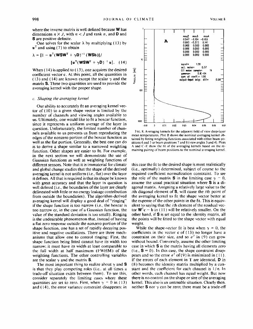
FIG. 8. Averaging kernels for the adjacent field of view deep-layer

mean temperatures. Plot B shows the nominal averaging kernel ob-

tained by tilting weighting functions associated with either beam po-

sitions 4 and 5 or beam positions 7 and 8 (view angles 3 and 4). Plots

A and C-E show the fit of the averaging kernels based on lhe re-

maining pairing of beam positions to the nominal averaging kernel.

this case the fit to the desired shape is most realistically(i.e., optimally) determined, subject of course to therequired coefficient normalization constraint. To seethe role of the matrix S in the limiting case 3" = 0,assume the usual practical situation where S is a di-agonal matrix. Assigning a relatively large value to theith diagonal element of S, will cause the ith point ofthe averaging kernel to fit the shape vector better atthe expense of the other points in the fit. This is equiv-alent to saying that the ith element of the residual vec-tor WTc - b in ( I 1 ) will be relatively smaller. On the

other hand, if S is set equal to the identity matrix, allthe points will be fitted to the shape vector with equalweight.

While the shape-vector fit is best when 3' = 0, thecoefficients in the vector c of (13) no longer have aconstraint on their size, and so a2 in (9) can growwithout bound. Conversely, assume the other limitingcase in which S is the matrix having all elements zero(i.e., S =- 0). In this case, the shape constraint disap-pears and so the error a 2 of(9) is minimized in ( 1 i ).If the errors of each element in T are identical, D in

(8) becomes the identity matrix multiplied by a con-stant and the coefficient for each channel is 1/n. Inother words, each channel has equal weight. But nowthere is no control on the shape or size of the averagingkernel. This also is an untenable situation. Clearly then,neither S nor 3' can be zero; there must be a trade-off

MAY 1995 GOLDBERG AND FLEMING 999

Ev

Lca-

I

:t- I

ii100 _- it

IOOO

l=Z

T 1 T [msu2 msu3 msu60.000 0.000 0.0000.741 -0.239 0.0330.712 -0.272 0.0250.000 0.000 0.0000.000 0.000 0.0000.000 0.000 0.000

starting/ending levels= 77 tO0pressures= 200.9 1000.0

sqcof= 1.19act. noise= 0.36

0.1 noise sample= 13gamma= O.IE-03sum of coeff.= 1.00

output-input intgr, dill= 11.70

E

=

-O.OI 0 0.01 002 0.03 0.04 0.05 0.06 0,07

I0 --

m

I00 --

m

D

1000 --

-0.01

I0

100

-- Ii

- I

1000 -- I-0.01 0 0.01

I I I I Imsu2 msu3 msu40.000 0.000 0.0000.000 0.000 0.0000.000 0.000 0.0002.366 -0.895 0.074

-0.927 0.396 -0.0150.000 0.000 0.000

sqcof= 7.62act. noise= 0.9003 noise sample= 81 --gamma= 0.1E-04 _sum of coeff.= 1.00

output-input int9r, di|f= -0.96--

m

....

0.07

E

o

m

10 P

m

100 --

I000

-001

FIG. 8. (('ontintted)

I

C

10.01

I

I I I Imsu2 msu3 msu40.000 0.000 0.0000.000 0.000 0.0001.478 -0.661 0.129

-O.OtO 0.124 -0.0600.000 0.000 0.0000.000 0.000 0.000

sqcof= 2.66act. noise= 0.540.1 noise sample= 29 -gamma= O.1E-04 _sum of coeff.= 1.00

output-input intgr, diff= -0.49-

u

002 0.03 004 0.05 0.06 0.07

I I I I Imsu2 msu3 msu40.000 0.000 0.0000.000 0.000 0.0000.000 0.000 0.0000.000 0.000 0.0003363 -0.469 0.001

-1.900 0.154 0.050

sqcof= 13.71act. noise= 1.230.1 noise sample= 150

gamma= O.IE-04sum of coeff.= 1.00

output-input intgr, diff=

0 0,01 0,02 0,03 0.04 0.05 0,06

m

-2.05--

0,07

between their magnitudes in order to achieve a satis-factory balance between an acceptable averaging kernelshape and an acceptable error level in the deep-layermean temperature.

The best strategy we found when using a boxcarconstraint is to define S as a diagonal matrix with valuesof zero in the nonzero elements of the boxcar and val-ues of one elsewhere. This will tend to force the aver-

aging kernel to be zero outside the boxcar. For a

Gaussian function, we found that simply defining S tobe the identity matrix produced desirable results. Thereason S is not critical for a Gaussian function is prob-

ably due to the smooth transition to zero from theGaussian's maxima. Figure 2 demonstrates the influ-ence of the "y parameter for fitting a Gaussian shapeconstraint (dashed curve) from MSU channels 2, 3,

and 4 weighting functions at all view angles. There aresix averaging kernels for six different values of 3'. The

1000 JOURNAL OF CLIMATE VOLUME8

E

cY_

100

I000

-OOl 0

I I I

0.01 0.02 0.0._ 0.04 005 0.06 0.07

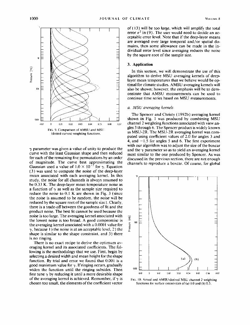
FroG. 9. Comparison of AMSU and MSU

(dotted curves) weighting functions.

3' parameter was given a value of unity to produce thecurve with the least Gaussian shape and then reducedfor each of the remaining five permutations by an orderof magnitude. The curve best approximating theGaussian used a value of 1.0 × l0 -7 for 3'. Equation(3) was used to compute the noise of the deep-layermean associated with each averaging kernel. In thisstudy, the noise for all channels is always assumed tobe 0.33 K. The deep-layer mean temperature noise asa function of y as well as the sample size required toreduce the noise to 0.1 K are shown in Fig. 3 (sincethe noise is assumed to be random, the noise will be

reduced by the square root of the sample size). Clearly,there is a trade-off between the goodness of fit and theproduct noise. The best fit cannot be used because thenoise is too large. The averaging kernel associated withthe lowest noise is too broad. A good compromise is

the averaging kernel associated with a 0.0001 value fory, because 1 ) the noise is at an acceptable level, 2) theshape is similar to the shape constraint, and 3) thereis no ringing.

There is no exact recipe to derive the optimum av-eraging kernel and its associated coefficients. The fol-lowing is the methodology that we use. First, begin byselecting a desired width and mean height for the shapefunction. By trial and error we found that 0.001 is agood maximum value for 3'. If ringing occurs, graduallywiden the function until the ringing subsides. Then

fine tune 3' by reducing it until a more desirable shapeof the averaging kernel is achieved. Remember, if 3' ischosen too small, the elements of the coefficient vector

of(13) will be too large, which will amplify the totalerror a: in (9). The user would need to decide an ac-ceptable error level. Note that if the deep-layer meansare averaged over large temporal and/or spatial do-mains, then some allowance can be made in the in-

dividual error level since averaging reduces the noiseby the square root of the sample size.

3. Application

In this section, we will demonstrate the use of thisalgorithm to derive MSU averaging kernels of deep-layer mean temperatures that we believe would be op-timal for climate studies. AMSU averaging kernels willalso be shown; however, the emphasis will be to dem-onstrate that AMSU measurements can be used tocontinue time series based on MSU measurements.

a. MSU averaging kernels

The Spencer and Christy (1992b) averaging kernelshown in Fig. 1 was produced by combining MSUchannel 2 weighting functions associated with view an-gles 3 through 6. The Spencer product is widely knownas MSU-2R. The MSU-2R averaging kernel was com-puted using coefficient values of 2.0 for angles 3 and4, and -1.5 for angles 5 and 6. The first experimentwith our algorithm was to adjust the size of the boxcarand the 3' parameter so as to yield an averaging kernelmost similar to the one produced by Spencer. As wasdiscussed in the previous section, there are not enoughchannels to reproduce a boxcar. Of course, for global

I i I I I I

E

100 _

- I I 4 _ ItI000 _--

-0.01 0 OOl 002 003 0.04

FIG. 10. Actual and kMSU-derived MSU channel 2 weighting

functions for surface emissivities of (a) 1.0 and (b) 0.5.

(b) il I

0.05 0.06 0.07

MAY I995 GOLDBERG AND FLEMING 1001

E

Lo-

100 __

IOO0 __

001

I I I I l l

0.01 0.02 0.03 0.0+ 005 0.06 0.07

FIG. I I. Actual and AMSU-derived MSU-2R averaging

kernels for surface emissivity of 1.0.

change purposes the averaging kernel does not have tobe a boxcar; all that is necessary is for the averagingkernel be known. Our averaging kernel is shown alongwith Spencer's (dotted curve) in Fig. 4. These averagingkernels are similar. The difference is that one was de-

termined subjectively and the other quantitatively usingthe algorithm of section 2. The numerical values inthe columns labeled msu2, msu3, and msu4 are thederived coefficients (i.e., the ci). Each channel is as-sociated with six coefficients, one for each view angle,beginning with view angle 1 (nadir). Hence, there is apotential maxima of 18 channels. It is seen that theonly nonzero coefficients are at view angles 3 through6 for channel 2. Also shown in the figure is the sum ofthe square of the coefficients, the noise of the product,the required sample size to reduce the noise of theproduct to 0.1 K, and the integrated difference in de-grees Kelvin. The integrated difference is scalar productof the difference between the shape vector and the de-rived averaging kernel vector and a standard midlati-rude temperature profile (vector). Note that the shapeconstraints and weighting functions used by the algo-rithm are defined at 100 levels equally spaced in logpressure.

The advantage of using an algorithm to objectivelydetermine the coefficients becomes quite clear if instead

of using four measurements to produce an averagingkernel, all 18 effective channels are considered. Forexample, the averaging kernel given by the solid curvein Fig. 5 was obtained by using all view angles of MSUchannels 2, 3, and 4, and hence all coefficients are non-

zero. This kernel is more desirable for monitoring tem-perature in the lower troposphere than the other av-eraging kernels shown in Fig. 4 since there is far lesssignal from the surface.

As participants in the NOAA/NASA Pathfinderprogram (Ohring and Dodge 1992), we are planningto construct time series of two types of deep-layer meantemperatures covering the entire MSU archive. We willprovide additional atmospheric layers to the ones givenby Spencer and colleagues. The first type is referred toas scan line products, since observations from all viewangles are to be used simultaneously. For the secondtype, observations from adjacent FOVs are used. Theremainder of this section is devoted to a discussion ofthese two product types.

The scan line products are derived from usingGaussian shape constraints. There will be a total of sixdifferent deep layers, their averaging kernels are shownin Fig. 6. The values of the product noise associatedwith the six averaging kernels beginning with the high-est peaking one are 0.89, 1.36, 0.76, 1.13, 0.62, and0.81 K. Each Gaussian function had a standard devia-

tion of six pressure levels, beginning at pressure level67 ( 100 mb) and were separated by six levels. The useof Gaussian curves for the shape vector has the advan-

tage that one can better dictate the location and shapeof the derived averaging kernel. Because of the limitednumber of channels on the MSU sounder, averagingkernels confined solely to the stratosphere cannot beprovided. Note that these averaging kernels are rela-tively narrow in comparison with the raw weighting

%-

c_

- t

z t10 --

100 --

I I I I I I

f

5> -

- i

,ooo- I 11_ I ....( i-oo_ o o.oi 002 0.03 0.04 0.05 0.06 oo7

FIG. 12. Example of nadir Gaussian-derived AMSU averaging

kernels in the troposphere and lower and upper stratosphere.

1002 JOURNAL OF CLIMATE VOLUME8

functions and could have been centered anywhere inthe troposphere without excessive ringing.

The scan line product's poor horizontal resolution,which is on the order of 1100 X 150 km 2 (the meanarea of scan line projected on the earth on either sideof nadir), results in relatively poor sampling. To mon-itor small temperature fluctuations, these products willneed to be averaged over relatively large spatial andtemporal domains to reduce the product noise. Onesuggestion is to average over 10° latitude bands andfor time intervals on the order of a month. The samplesize will be about 10 000 (assumes 2 products per scanline, 220 scan lines per orbit, 14 orbits per day). Thesingle largest product noise of 1.36 K will be reducedto a precision of 0.0136 K.

For regional climate monitoring the horizontal res-olution of the product needs to be much smaller. Todo this we want to derive products that are ideally based

on a single FOV. In other words, I 1 products for the11 FOVs along the MSU scan line. There are differentways to do this. To apply the same set of coefficientsto all view angles, the off-nadir measurements need tobe adjusted to look as if they were observed at nadir(i.e., limb correct the measurements). For example,one can collect a large ensemble of measurements forall FOVs and compute regression coefficients using themeasurements observed at a given FOV as the predic-tors and measurements observed at nadir as the pre-dictands (Wark 1993). The MSU-2 and MSU-4 timeseries given in Spencer and Christy ( 1992a, 1993 ), re-spectively, were limb corrected.

Our approach is not to use a statistical method tolimb correct, since we believe it is undesirable to adjustthe measurements based on historical data. An attempt

was made to physically limb correct the MSU by usingthe algorithm to compute coefficients for combiningweighting functions at a particular off-nadir view angleto fit the nadir-viewing weighting functions. Unfortu-nately, this technique did not work well at the largerview angles. We also tried to compute a different setof coefficients for each view angle in order to fit a com-mon averaging kernel. However, a combination basedon only three channels was insufficient to maintain thesame averaging kernel along the scan line. The solutionwas to use information from a pair of adjacent FOVs,

which provides a total of six weighting functions to fitthe desired averaging kernel. To better visualize thisapproach, the MSU scan line geometry and the adja-cent FOVs used to yield the ten deep-layer mean tem-perature products across each scan is given in Fig. 7.So instead of a two products per scan line, this tech-nique yields ten products. The nominal averaging ker-nel (dotted curve) is shown in plot B of Fig. 8. Thisaveraging kernel was derived from a boxcar constraintand used weighting functions from view angles 2 and3, which corresponds either to field of view 4 and 5 or7 and 8. The nominal averaging kernel was then usedas a shape constraint for other angular combinations

g

&

\

Im

t,

-- (_ - I

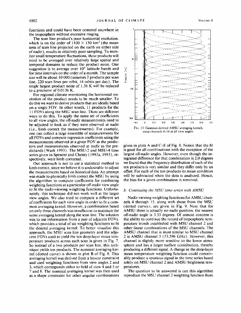
-0.o_ ool 002 oo_ oo4 oos oo_

FIG. I 3. Oaussian-derived AMSU averaging kernels

using channels 4-14 at all view angles.

given in plots A and C-E of Fig. 8. Notice that the fitis good for all combinations with the exception of thelargest off-nadir angles. However, even though the in-tegrated difference for that combination is 2.0 degreeswe found that the frequency distribution of each of theten products is very similar and they differ only by anoffset. For each of the ten products its mean conditionwill be subtracted when the data is analyzed. Hence,the bias for a given combination is removed.

b. Continuing the MSU time series with AMSU

Nadir-viewing weighting functions for AMSU chan-nels 4 through 15, along with those from the MSU(dotted curves), are given in Fig. 9. Note that forAMSU there is actually no nadir position, the nearestoff-nadir angle is 3.33 degrees. Of utmost concern isthe ability to continue the record of tropospheric tem-perature trends established with MSU channel 2 andother linear combinations of the MSU channels. TheAMSU channel that is most similar to MSU channel2 is AMSU channel 5 (53.596 GHz). However, thischannel is slightly more sensitive to the lower atmo-sphere and has a larger surface contribution, therebyproducing a different signal. A change in the deep-layermean temperature weighting function could conceiv-ably produce a spurious signal in the time series basedsolely on MSU channel 2 and AMSU brightness tem-peratures.

The question to be answered is can this algorithmreproduce the MSU channel 2 weighting function from

MAY I995 GOLDBERG AND FLEMING 1003

the AMSU channel weighting functions? The answerto this question is yes. In Fig. 10 there are four curves.The curves to the left are the actual MSU channel 2

(solid curve) and the AMSU reconstructed MSUchannel 2 (dotted curve) for a surface emissivity of1.0. The other set of curves is for an emissivity of 0.5.

The shape is different because the emissivity enters intothe computation of the weighting functions. Only the"nadir" AMSU channels 4 through 7 weighting func-tions were used in deriving the coefficients. The selectedemissivities are the extremes values for the surface

emissivity in the 50-GHz band. The actual and recon-structed MSU channel 2 weighting functions are vir-tually identical. It is very important to note that thecoefficients, based on an emissivity of 1.0, were usedfor reconstructing the weighting functions for an emis-

sivity of 0.5. In other words, the reconstruction of MSUchannel 2 is insensitive to surface emissivity, which isvery important since the estimation of surface emis-sivity would add uncertainty to the final product. Byusing the appropriate y, the integrated error betweenthe real and reconstructed MSU channel 2 weightingfunction can be forced to be virtually zero. If we did

nothing and simply used AMSU channel 5 to continueMSU channel 2, there would be a sizable airmass de-pendent bias. For a summer midlatitude atmosphere,the bias would be about 5.6 K. The linear combination

of AMSU to yield an equivalent MSU channel 2 mea-surement is

7m_,2 = -0.0488T_ .... 4 + 0.932T, m_o5

+ 0.20g/amour -- 0.466T, .... 7. (15)

Spencer's MSU-2R product can also be reproducedfrom the AMSU. AMSU channels 4 through 8 using10 angles ranging from 18.66 to 49.55 degrees werecombined to fit the MSU-2R averaging kernel. TheAMSU equivalence of MSU-2R is given in Fig. 11.The coefficients are obtainable from the author.

Even though the accuracy of fitting AMSU to MSUappears to be high, the underlying assumption is thatthe weighting functions are known exactly. In practice,we know this is not true. Therefore, in conjunctionwith this algorithm, overlap of MSU and AMSU willbe needed to adjust for the component that is left overafter the "known" physics have been accounted for.

The AMSU by itself will be a very important sensorfor monitoring temperature trends throughout the at-mosphere. Its numerous channels will enable one tomonitor temperature in three important regions of theatmosphere: the upper and lower stratosphere and thetroposphere. Figure 12 shows examples of AMSU av-eraging kernels in these three regions. All were derivedfrom initial Gaussian curves using only nadir mea-surements. Narrower averaging kernels can be achievedby utilizing off-nadir measurements. The techniqueused to generate the six averaging kernels, shown inFig. 6, was applied to AMSU channels 5 through 14

weighting functions at all view angles. The result,shown in Fig. 13, clearly demonstrates that the abilityto derive these averaging kernels is no longer restrictedto the troposphere. It is also important to mention that

the lowest six averaging kernels in Fig. 13 are virtuallyidentical to the six averaging kernels shown in Fig. 6.Therefore, in addition to Spencer's time series of MSU,we will be able to extend our own time series withAMSU.

4. Summary

An algorithm for deriving deep-layer mean temper-atures from microwave sensors has been developed.The algorithm, in conjunction with the microwavechannels considered in this study, is completely inde-pendent of a priori information. Independence fromancillary data is critical for high-precision monitoringof climate trends, so that any observed trends in thedeep-layer mean temperatures are attributed only totrends in the sensor's measurements. The algorithmalso has been shown to be capable of combining mea-surements from next-generation microwave sensors toreconstruct measurements from current sensors. This

enables one to generate continuous time series of sat-ellite-derived temperature trends accurately, regardlessof changes in satellite instrumentation.

The next step is to produce the actual MSU timeseries from the two types of deep-layer mean temper-atures we plan to derive as part of the TOVS Pathfinderproject. The first type will yield six different atmo-spheric deep-layer mean temperatures: their averagingkernels were shown in Fig. 6. The second type usesadjacent angular combinations to yield a single at-mospheric averaging kernel. The important feature ofthe second type is that for each adjacent combination,the averaging kernel along the scan line is preservedso that limb correcting the measurements can beavoided.

Acknowledgments. The first author would like to ac-knowledge the appreciation of the nearly 10 years ofcollaboration with Henry E. Fleming. Henry was notonly a respected colleague but also a good friend. Henrypassed away on 8 November, 1992. This work repre-sents our final collaboration, l would also like to ac-

knowledge David Crosby, another colleague and goodfriend of Henry, for his many suggestions in prepara-tion of this manuscript. This work was partially fundedby the NOAA/NASA TOVS Pathfinder Program.

REFERENCES

Conrath, B., 1972: Vertical resolution of temperature profiles obtained

from remote sensing measurements. J ..Itmos Sci., 29, 1261-1272.

Eyre, J. R., 1989: lnvcrsion of cloudy radiances by nonlinear oplimal

estimation I: Theory and simulation for TOVS. Quart. J. Ro.v.Meteor. Sot., 115, 1001-1026.

Fischer, J, C., 1987: Passive microwave observing lbrm environmental

satellites, A status report based on NOAA's June 1-4, 1987.

1004 JOURNAL OF CLIMATE VOI_UME8

NOAA Tech. Rep. NESDIS 35, conference in Williamsburg,

VA, 292 pp.

Fleming, H. E., M. D. Goldberg, and D. S. Crosby, 1988: Oper-

ational implementation of the minimum variance simulta-neous method. Preprints, Third Con[_ on Satellite Meteorol-

ogy and Oceanography, Anaheim, CA, Amer. Meteor. Soc.,16-19.

Goldberg, M. D., J. M. Daniels, and H. E. Fleming, 1988: A method

for obtaining an improved initial approximation for the tem-

perature/moisture retrieval problem. Preprints, Third ConJ. on

Satellite Meteoroh_gy and Oceanography. Anaheim, CA, Amer.Meteor. Soc., 20-23.

Hayden, C. M., 1988: GOES-VAS simultaneous temperature-mois-

ture retrieval algorithm. J. AppL Meteor. 27, 705-733.Mitchell, J. F. B., S. Manabe, V. Meleshko, T. Tokioka, 1990:

Equilibrium climate change--and its implications for the fu-ture. Climate Change. The IPCC Scient(tic Assessment,

World Meteorological Organization, Houghton, J. T., G. J.

Jenkins, and J. J. Ephrams, Eds, Cambridge University Press,131-172,

Ohring, G., J. C. Dodge, 1992: The NOAA/NASA pathfinder pro-

gram. Int. Radiation S)'mp., Keevallik and Karner, Eds., Deepak,405-408.

Spencer, R. W., and J. R. Christy, 1992a: Precision and radiosonde

validation of satellite gridpoint temperature anomalies, Part 1:

MSU channel 2. J. (_Timate, 5, 847-857.-, and --, 1992b: Precision and radiosonde validation of sat-

ellite gridpoint temperature anomalies, Part 2: A troposphericretrieval and trends during 1979-90. J. Climate, 5, 858-866.

---, and ---, 1993: Precision lower stratospheric temperature

monitoring with the MSU: Technique, validation, and results

1979-1991. J. Climate, 6, 1194-1204.

--, --, and N. C. Grody, 1990: Global atmospheric temperature

monitoring with satellite microwave measurements: Method and

results 1979-1984. J. Climate, 3, 1111-1128.

Thompson, O. E., and M. T. Tripputi, 1994: NWP initialized satellite

temperature retrievals using statistical regularization and singular

value decomposition. Mon. H.2,a. Rev.. 122, 897-926.Wark, D. Q., 1993: Adjustment of TIROS operational vertical sounder

data to a vertical view. NOAA Tech. Rep. NESDIS 64, 36 pp.