An algebraic approach to Integer Portfolioproblems

F. Castro J. Gago I. Hartillo J. PuertoJ.M. Ucha

Abstract

Integer variables allow the treatment of some portfolio optimiza-tion problems in a more realistic way and introduce the possibility ofadding some natural features to the model.

We propose an algebraic approach to maximize the expected re-turn under a given admissible level of risk measured by the covariancematrix. To reach an optimal portfolio it is an essential ingredientthe computation of different test sets (via Grobner basis) of linearsubproblems that are used in a dual search strategy.

1 Introduction

Mean-variance portfolio construction lies at the heart of modern asset man-agement and has been among the most investigated fields in the economicand financial literature. The classical Markowitz’s approach, cf. [Mar52],or [Mar00] for a recent reissue of his work, rests on the assumption that in-vestors choose among n risky assets to look for their corresponding weightswi in their portfolios, on the basis of

1. previously estimated expected returns µi, and

2. the corresponding risk of the portfolio measured by the covariance ma-trix Ω.

Portfolios are considered mean-variance efficient in two senses:

1

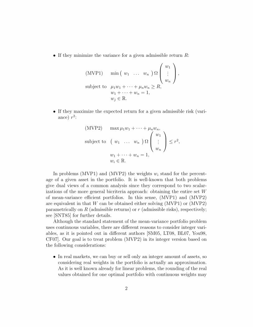
• If they minimize the variance for a given admissible return R:

(MVP1) min(w1 . . . wn

)Ω

w1...wn

,

subject to µ1w1 + · · ·+ µnwn ≥ R,w1 + · · ·+ wn = 1,wj ∈ R.

• If they maximize the expected return for a given admissible risk (vari-ance) r2:

(MVP2) maxµ1w1 + · · ·+ µnwn,

subject to(w1 . . . wn

)Ω

w1...wn

≤ r2,

w1 + · · ·+ wn = 1,wi ∈ R.

In problems (MVP1) and (MVP2) the weights wi stand for the percent-age of a given asset in the portfolio. It is well-known that both problemsgive dual views of a common analysis since they correspond to two scalar-izations of the more general bicriteria approach: obtaining the entire set Wof mean-variance efficient portfolios. In this sense, (MVP1) and (MVP2)are equivalent in that W can be obtained either solving (MVP1) or (MVP2)parametrically on R (admissible returns) or r (admissible risks), respectively;see [SNT85] for further details.

Although the standard statement of the mean-variance portfolio problemuses continuous variables, there are different reasons to consider integer vari-ables, as it is pointed out in different authors [SM05, LT08, BL07, You98,CF07]. Our goal is to treat problem (MVP2) in its integer version based onthe following considerations:

• In real markets, we can buy or sell only an integer amount of assets, soconsidering real weights in the portfolio is actually an approximation.As it is well known already for linear problems, the rounding of the realvalues obtained for one optimal portfolio with continuous weights may

2

produce, in principle, an infeasible solution or a very bad approximationto the optimal integer solution. We think that this is indeed the casefor a portfolio that potentially considers future contracts, as in [GK08]for commodity futures, to obtain lower correlations concluding on thebenefits of diversification. We show this behaviour in Example 5.2.

• The need to diversify the investments in a number of industrial sectors[BL07].

• The constraint of buying stocks by lots [BL07, CF07, JHLM01].

• Another reason for the use of integer variables, usually binary, appearsin practice because portfolio managers and their clients often hate smallactive positions and very large number of assets, the reason being thatthey produce big transaction and monitoring costs. Hence it is ratherusual to add the constraints associated to the following conditions:

1. there should be at least some previously decided minimum per-centage (lower bounds), and

2. there should be a maximum number of assets (upper bounds).

Furthermore, transaction costs are included as linear constraints in thereturn equation, using decision variables, as in [LT08].

The above mentioned requirements enrich any portfolio model for real ap-plications and require 0-1 or, more generally, integer variables. Nevertheless,as far as we know there are no specific algorithms to solve these problems.Note that methods in semi-definite programming deal with this problem, butthey are oriented to the continuous case. See also [SM05] for a set of routinesthat handles these problems in the continuous case. In our approach, it isnatural to consider non negative integer variables x1, . . . , xn for the quantitiesof each product. Then it is necessary to take into account

• the unit prices a1, . . . , an of the products,

• the expected returns of each stock µ1, . . . , µn,

• and the total available budget B.

3

Then Problem (MVP2), in its integer version, can be restated as

max∑n

i=1 µixi = µtxsubject to

∑ni=1 aixi = atx ≤ B,

Q(x) ≤ B2r2,x ∈ (Z+)n,

where

Q(x) =(a1x1 . . . anxn

)Ω

a1x1...

anxn

.

1.1 Previous works and our approach

There have been several works with different techniques to treat Problem(MVP1) in an integer framework.

• For (MVP1): piecewise linear approximation in [Sha71] and [Sto73],absolute deviation selection in [YK91], branch-and-cut techniques in[Bie96] and minimax selection approach in [You98].

• For (MVP1) with additional transaction cost: dual Lagrangian relax-ation in [MM91, GK87], linear terms transformation in [LC98], sepa-rable terms transformation in [Sha71, Sto73], and parallel distributedcomputation reformulating the objective function into an ellipse andusing piecewise linearization in [LT08].

For Problem (MVP2) the literature is not so wide, although this ap-proach is very usual in practice for the so called benchmark portfolios, asused in [MM08]. The results of [BPT00] have been in some sense a milestonein applying tools of Algebraic Geometry (namely Grobner bases) to opti-mization, although this method is not effective for Problem (MVP2). See[AL94, Ch.1,2], [CLO05, Ch. 2], or [BW05] for introductions to this subject.

Our goal is to present a new algorithm to deal with portfolio problemswith integer variables and non-linear constraints. The method is based onthe computation of some test sets using Grobner bases. These bases are com-puted from a linear integer subproblem that contains the original linear con-straints together with some new cuts induced by the non-linear constraints.The use of the reversal test-set allows us to design a dual search algorithm

4

that moves from the optimal solution of the linear subproblems towards theoptimal solution of the entire portfolio problem. Our approach is new withrespect to the cited references, and we will see in the last section that it iseffective to deal with portfolios with number of stocks comparable to thosein the literature (see [CF07, LT08]).

The paper is organized as follows. In Section 2 we fix the formulationof the problem to be treated with the method explained in [TTN95]. InSection 3 the successive additions of linear constraints are explained, and thedual search algorithm based on a test-set computed from a Grobner basisis applied to find an optimal point of Problem (1). It is also included anillustrative example.

Section 4 explains the existence of a lower bound r2b to the risk value r2

below that it is not necessary to invest the whole budget to get an optimalportfolio. Section 5 contains some computational experiments and Section 6draws some conclusions on the paper.

2 Preliminaries

If one accepts the integer version of model (MVP2) to obtain efficient portfo-lios, the objective function and all constraints but one —that is quadratic—are linear. This is related to the form of the problem treated in [TTN95]. Tosolve an integer programming problem (P) with linear objective function un-der different linear and nonlinear constraints, the following general approachcan be applied (see [TTN95] for a complete example):

1. First obtain a test-set for a linear part of (P), let us call it (P′). Atest-set T is a set of vectors in Zn such that, given a feasible point F of(P′), if none of the feasible points obtained adding the elements of T toF improves the value of the objective function, then F is an optimumof (P′). A test-set of a linear integer problem can be obtained viaGrobner bases ([CT91], see [Stu96, ch. 5] for a modern introduction).

The best known way of obtaining these bases is using programs as4ti2 ([tt08]), that takes advantage of the special structure of the toricideals corresponding to linear integer problems. Programs for generalGrobner bases are not so good for big examples.

2. Starting at the optimum of the linear problem (P′), which is possiblyan infeasible point for problem (P), use the reversal test-set —so de-

5

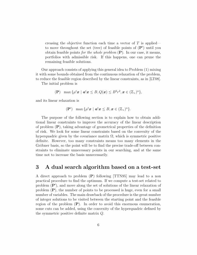
creasing the objective function each time a vector of T is applied—to move throughout the set (tree) of feasible points of (P′) until youobtain feasible points for the whole problem (P). In our case, it means,portfolios with admissible risk. If this happens, one can prune theremaining feasible solutions.

Our approach consists of applying this general idea to Problem (1) mixingit with some bounds obtained from the continuous relaxation of the problem,to reduce the feasible region described by the linear constraints, as in [LT08].

The initial problem is

(P) max µtx | atx ≤ B,Q(x) ≤ B2r2,x ∈ (Z+)n,

and its linear relaxation is

(P′) max µtx | atx ≤ B,x ∈ (Z+)n.

The purpose of the following section is to explain how to obtain addi-tional linear constraints to improve the accuracy of the linear descriptionof problem (P), taking advantage of geometrical properties of the definitionof risk. We look for some linear constraints based on the convexity of thehyperquadric given by the covariance matrix Ω, which is symmetric positivedefinite. However, too many constraints means too many elements in theGrobner basis, so the point will be to find the precise trade-off between con-straints to eliminate unnecessary points in our searching, and at the sametime not to increase the basis unnecessarily.

3 A dual search algorithm based on a test-set

A direct approach to problem (P) following [TTN95] may lead to a nonpractical procedure to find the optimum. If we compute a test-set related toproblem (P′), and move along the set of solutions of the linear relaxation ofproblem (P), the number of points to be processed is huge, even for a smallnumber of variables. The main drawback of the procedure is the great numberof integer solutions to be visited between the starting point and the feasibleregion of the problem (P). In order to avoid this enormous enumeration,some cuts can be added, using the convexity of the hyperquadric defined bythe symmetric positive definite matrix Q.

6

We assume that a black box is available providing solutions to linearcontinuous optimization problems with quadratic convex constraints, as thefunction fmincon in Matlab, the different implementations of semi-definiteprogramming compared in [Mit03], or even the linear time in fixed dimensionalgorithm by [Dye92].

3.1 Starting tasks

In order to improve our representation of problem (P), we proceed as follows:

• The first step is the computation of the continuous solution uc of theproblem

max µtx | atx ≤ B,Q(x) ≤ B2r2,x ∈ (R+)n,

which gives us a return µtuc = Rc. Clearly the discrete return isless than or equal to bRcc (function ComputeContinuousOptimum inAlgorithm 1).

• Secondly, we need a good discrete feasible point, which will give us alower bound for the return. The problem (P) is always feasible, becausethe origin belongs to the region, but this point it is not very useful. Therounded point ud = bucc is not always feasible, as it is well-known.

• In order to get a feasible starting point, it is possible to decrease eachcoordinate until we get a feasible point. After that, the point can beimproved so that the return cannot be increased in any direction insidethe feasible region (function ComputeDiscreteApprox in Algorithm 1).

From this point pe we will reach the discrete optimum. Let Re = µtpe be thereturn associated with the discrete feasible point pe. A new valid formulationof the problem is

max µtx | atx ≤ B,Re ≤ µtx ≤ bRcc, Q(x) ≤ B2r2,x ∈ (Z+)n.

3.2 Addition of new linear constraints

From the above formulation, we improve our description of problem (P) intwo ways.

7

1. Adjusting hyperplanes to the hyperquadric given by upper and lowerbounds on the variables.

To this end, for j = 1, . . . , n, we solve the continuous problems (func-tion ComputeLowerBounds in Algorithm 1)

min xj | atx ≤ B,Re ≤ µtx ≤ bRcc, Q(x) ≤ B2r2,x ∈ (R+)n.

The above minimum values give us an integer lower bound bj for eachvariable xj, applying the ceiling function. The constraints bj ≤ xj arenot going to be involved in the computation of the test-set throughthe Grobner basis. This is because we can write bj + yj = xj, whereyj ≥ 0, and this change of variables do not alter the coefficient matrixof the linear cuts, nor the linear cost function. Since the computationof the Grobner basis does depend only of this matrix, there is no extracomputation time.

In a similar way, the maximization problems

max xj | atx ≤ B,Re ≤ µtx ≤ bRcc, Q(x) ≤ B2r2,x ∈ (R+)n

for j = 1, . . . , n, provides us upper bounds. However, these linearconstraints highly increase the size of the test-set. We will only usethem to fix variables, because the upper and lower bounds of somevariables are equal in many examples. This fact allows us reducing thedimensionality of the problem.

We consider the polytope

P = x ∈ Rn | atx ≤ B,µtx ≤ bRcc,µtx ≥ Re, b ≤ x

where b ≤ x stands for the conditions bi ≤ xi, i = 1, . . . , n.

2. Adding nearly tangent hyperplanes to shrink the polytope.

The main idea is the addition of cuts so that the farthest regions of thepolytope P could be cut off. To do that, we use a point of P wherethe function Q takes its greatest value. This is equivalent to solve thecontinuous problem

max Q(x) | x ∈ P.It is coded as function ComputeMaxRisk in Procedure NewPolytope.Note that this problem can be efficiently solved since it is of polynomialcomplexity [KTH79].

8

Let pmax be a solution of Problem (2), s be the half-line from thefeasible point pe to pmax, and p′ = Q ∩ s the intersection point of swith the hyperquadric Q defined by the function Q(x) = B2r2.

Let H be the supporting hyperplane to Q at the point p′. By the con-vexity of Q, the hyperplane H defines a linear half-space that containsthe interior of Q.

The coefficients of the hyperplane H are real numbers, so its normalvector nmay have non integer components. However, we are looking forlinear constraints with integer coefficients, so we round the vector n toan integer vector n ∈ Zn (variable Prec in Procedure NewPolytope).Then we proceed to compute the independent term c of the tangenthyperplane to Q whose normal vector is equal to n, and such that thehalf-space ntx ≤ c = dce defines a linear half-space which contains theinterior of Q.

This process can be iterated as many times as we wish (AlgorithmNewPolytope), shrinking the polytope P . Nevertheless, there shouldbe a trade-off between the number of new hyperplanes and the size ofthe Grobner basis associated with the system, so the maximum numberof cuts allowed is a parameter of the algorithm. Additionally, the differ-ence between r2m = maxQ(x) | x ∈ P and the initial risk r20 is anotherstopping criterion, passed as the parameter Tol to the algorithm.

3.3 Dual iterations with the test-set

Now after the above two phases Problem 1 is transformed to

maxµtxs. t. atx ≤ B,

Re ≤ µtx ≤ bRcc,nt

kx ≤ ck, k = 1, . . . , s,x ≥ b,x ∈∈ (Z+)n,Q(x) ≤ B2r2,

9

where ntkx ≤ ck, k = 1, . . . , s are the new cuts. The test-set G is associated

with the linear problem

maxµtxs. t. atx ≤ B,

µtx ≤ bRcc,nt

kx ≤ ck, k = 1, . . . , s,x ≥ b,x ∈ (Z+)n.

The condition Re ≤ µtx is tested inside the tree-search, and used to pruneleaves. The value of Re is updated as soon as a new feasible point with abetter return is found.

Once we have the test-set of the above polytope we proceed with theresolution method. The main bottleneck of our approach is the search overthe tree defined by the test-set. The number of points to be processed isstrongly related to the initial feasible point pe found because:

1. The estimated return Re defines the lowest facet of the polytope P interms of the objective value.

2. The upper and lower bounds for the variables xi are strongly deter-mined by Re. The closer is Re to the optimal value, the narrower is theinterval for each variable xi.

On the other hand, to apply the reversal test-set search we need an ini-tial (and usually non feasible) point, but not far from feasibility. We takethe point pbounds built by considering the independent terms of the linearconstraints of Problem (3.3), after applying the translation bi + yi = xi, i.e.,

pbounds = (b, B − atb, bRcc − µtb, ck − ntb)t.

The starting point for the reversal test-set tree search is the point pini, thereduced of pbounds by the test-set G. This is the solution of the linear problem(3.3), as shown in [CT91]. With the reversal test-set, we search over the treeof nodes (feasible points for the linear problem) until we obtain a feasiblepoint for the entire problem, including the quadratic constraint (functionTreeSearch in Algorithm 1). If the switch SwFictBounds is set to true, thesearch is stopped in the first point that improves the estimated return givenby the incumbent point pe.

10

Although the tree search has to end, a maximum number of processedrecords is passed to the procedure TreeSearch as a parameter. It couldhappen that the number of points processed exceeds the maximum allowed,and the optimum had not been found. If a new feasible point p′e is found(SwImprove = true), the bounds can be recomputed. The test-set is stillvalid for the new search. The only new computations are the independentterms of the hyperplanes and the reduction to find the starting point.

However, if the test-set were huge, it would be better to compute the newlinear cuts given by the new estimated point p′e and its associated Grobnerbasis. In general, the Grobner basis will be shorter, and the elapsed timespent in the tree search will be shortened.

3.4 Restricted search in a region

In the case that a new feasible point is not found after a given number ofprocessed points (SwImprove = false), it is then possible to apply a branch-and-cut technique with the bounds. Indeed, let pe be the feasible pointthat gives the value Re, and b the vector of lower bounds for the variablesxi, i = 1, . . . , n. Compute a point b′ = b + α(pe − b), 0 < α < 1 (usuallyα = 1/2), which we call fictitious bound, and consider the following problem:

maxµtxs. t. atx ≤ B,

Re ≤ µtx ≤ bRcc,nt

kx ≤ ck, k = 1, . . . , s,x ≥ b′,x ∈ (Z+)n,Q(x) ≤ B2r2.

(1)

Solving the above problem, we expect to find a new feasible point to relaunchthe search process. The idea is simple: the search is restricted to a smallerregion, but the solution of the original problem is not guaranteed to be inthat region. It is a heuristic technique to take advantage that this newproblem does not need a new test-set. In our implementation, this searchcan be launched by setting the switch SwFictBounds equal to true. Theprocess is stopped as soon as a new point is found, and then we start again.If no point is found after the maximum number of allowed nodes (variableMaxNumNodes in Algorithm 1), then we stop, and the point pe is our bestvalue.

11

The pseudocode of the main algorithm is described in DiscreteOptimum.The procedure NewPolytope presents the pseudocode of the strengthening ofthe polytope P by adding valid cuts. The switch SwEOP is used to markthe end of the process.

3.5 An illustrative example

Let a = (6075, 3105)t be the vector of prices, and µ = (12500, 10000)t thevector of returns, with the covariance matrix equals to

Ω =

(.832843e− 4 .485325e− 4.485325e− 4 .651298e− 3

).

Let B = 9 × 106 be the budget, and r2 = 3 × 10−5 the fixed risk. Thecontinuous optimum is uc = (772.754778, 215.028056)t, with a total returnRc = 11809715.29. Then bRcc = 11809715, and rounding uc we get thepoint ud = (773, 215), which is not a feasible point. Subtracting from thecomponents, we eventually reach a feasible point pe = (773, 214), whoseassociated return is Re = 11802500. The lower bounds b1 and b2 are nowcomputed, solving first the continuous problems

min xi | atx ≤ B,Re ≤ µtx ≤ Rc, Q(x) ≤ r2B2,x ∈ (R+)2,

where

Q(x) =(a1x1 a2x2

)Ω

(a1x1a2x2

). (2)

The respective continuous values are b1 = 752.69, rounded to b1 = 753, andb2 = 190.58, rounded to b2 = 191. We want to solve the problem

max µtx | atx ≤ B,Re ≤ µtx ≤ bRcc, Q(x) ≤ r2B2,x ≥ b,x ∈ (Z+)2.

In the associated linear problem

max µtx | µtx+ z1 = bRcc,atx+ z2 = B,x ≥ b,x ∈ (Z+)2

we change the variables xi = yi + bi, and the resulting linear problem has thesame coefficient matrix. The computation of a Grobner basis leads to thetest-set formed by vectors

v1 = (−4, 5, 8775, 0)t, v2 = (−1, 1, 2970, 2500)t, v3 = (0,−1, 3105, 10000)t,v4 = (1,−2, 135, 7500)t, v5 = (2,−3,−2835, 5000)t, v6 = (3,−4,−5805, 2500)t.

12

Now, we reduce the point

pbounds = (b1, b2, B−a1b1−a2b2, bRcc−µ1b1−µ2b2)t = (753, 191, 3832470, 487215)t

with the test-set to get the linear problem optimum, which is the startingpoint pini of the tree search. In this case, pini = (791, 192, 3598515, 2215). Wenow show the path followed by the search procedure in the tree of solutionsof the linear part of the problem. In each node, we write the distance ∆1 tothe continuous return associated with it, that is, ∆1 = bRcc − µt(p + vi).The initial distance is ∆e = 7215, the difference between bRcc and Re. Thelarger the value, the smaller the return. Therefore, values larger than ∆e

means that the corresponding branch can be pruned. The list of nodes tobe processed are then ordered by ∆1. Note that black dots ‘•’ mean prunednodes, and white dots ‘’ mean new nodes. The points are shortened to thetwo first components to save space.

? Node p = (791, 192)t,∆e = 7215. Leaves p+ vi, i = 1, . . . , 6:

– p+ v1 = (787, 197)t,∆1 = 2215, r2 ≥ r20. New node .– p+ v2 = (790, 193)t,∆1 = 4715, r2 ≥ r20. New node .– p+ v3 = (791, 191)t,∆1 = 12215 > ∆e. Pruned by ∆e.

– p+ v4 = (792, 190)t,∆1 = 9715. Pruned by bound b2 = 191.

– p+ v5 = (793, 189)t,∆1 = 7215. Pruned by bound b2 = 191.

– p+ v6 = (794, 188)t,∆1 = 4715. Pruned by bound b2 = 191.

The above information gives rise to the following descendants.

(791, 192)

'' ++ ,, --

// •(794, 188)

(787, 197) (790, 193) •(791, 191) •(792, 190) •(793, 189)

List of ordered nodes: (787, 197)t, (790, 193)t.

? Node p = (787, 197)t,∆e = 7215. Leaves p+ vi, i = 1, . . . , 6:

– p+ v1 = (783, 202)t,∆1 = 2215, r2 ≥ r20. New node .– p+ v2 = (786, 198)t,∆1 = 4715, r2 ≥ r20. New node .

13

– p+ v3 = (787, 196)t,∆1 = 12215 > ∆e. Pruned by ∆e.

– p+ v4 = (788, 195)t,∆1 = 9715 > ∆e. Pruned by ∆e.

– p+ v5 = (789, 194)t,∆1 = 7215 = ∆e. Pruned by ∆e.

– p+ v6 = (790, 193)t. Already in the list of nodes to be processed.

The corresponding diagram is displayed as

(787, 197)

'' ++ ,, --

// •(790, 193)

(783, 202) (786, 198) •(787, 196) •(788, 195) •(789, 194)

List of ordered nodes (783, 202)t, (786, 198)t, (790, 193)t.

? Node p = (783, 202)t,∆e = 7215. Leaves p+ vi, i = 1, . . . , 6:

– p + v1 = (779, 207)t , ∆1 = 2215 < ∆e, r2 ≤ r20. Feasible point,

and improvement. Update ∆e = 2215.

– p+ v2 = (782, 203)t,∆1 = 4715 > ∆e. Pruned by ∆e.

– p+ v3 = (783, 201)t,∆1 = 12215 > ∆e. Pruned by ∆e.

– p+ v4 = (784, 200)t,∆1 = 9715 > ∆e. Pruned by ∆e.

– p+ v5 = (785, 199)t,∆1 = 7215 > ∆e. Pruned by ∆e.

– p+v6 = (786, 198)t,∆1 = 4715 > ∆e. Deleted of the list of nodesto be processed.

The tree representation is

(783, 202)

'' ++ ,, --

// •(786, 198)

(779, 207) •(782, 203) •(783, 201) •(784, 200) •(785, 199)

List of ordered nodes (790, 193)t.

? Node p = (790, 193)t. This node is pruned because ∆1 > ∆e, so theprocess is finished. The total number of processed nodes is 4.

14

The optimum is (779, 207)t, with a difference return of 2215 units from thecontinuous solution. The initial estimated point was at 7215 units. This ex-ample shows a large difference between the rounded solution and the discreteoptimum.

Although this example is very simple, we will now show the improvementthat we get using the cuts. The initial polytope P is defined by

P = x ∈ Rn | atx ≤ B,Re ≤ µtx ≤ bRcc,x ≥ b.

The first maximum of the quadric Q(x) described in Equation (2) onthe polytope is pmax = (753, 479443

2000)t and the tangent line at the intersection

point has as normal vector (0.54452, 0.45547)t. Rounding to three digits,the new normal vector of the hyperplane is (545, 455)t, and the independentterm is 519113.7265. Then the first cut is 545x1 + 455x2 ≤ 519114. Addingthis inequality to the polytope P , and repeating the process, we have thenew maximum at point pmax = (1979943

2500, 191)t, and the normal vector of the

tangent cut is equal to (0.56698, 0.43301)t. Then the new cut is 567x1 +433x2 ≤ 531402.

The linear problem, with the slack variables considered, is

maxµtxs. t. µtx+ z1 = bRcc,

atx+ z2 = B,x ≥ b,545x1 + 455x2 + z3 = 519114,567x1 + 433x2 + z4 = 531402,

and the test-set associated with it has 7 elements:

w1 = (−4, 5, 8775, 0,−95, 103)t, w2 = (−1, 1, 2970, 2500, 90, 134)t,w3 = (0,−1, 3105, 10000, 455, 433)t, w4 = (1,−2, 135, 7500, 365, 299)t,w5 = (2,−3,−2835, 5000, 275, 165)t, w6 = (3,−4,−5805, 2500, 185, 31)t,w7 = (7,−9,−14580, 2500, 280,−72)t.

The starting point pini is the reduction of the point

pbounds = (753, 191, 3832470, 487215, 21824, 21748)t

with the test-set. In this case, pini = (779,207, 3624840, 2215, 374, 78)t, andit is already the optimum point.

15

In this example, there is a large amount of money (value 3624840) that isnot invested. The explanation of this counterintuitive behaviour is becausethe risk r2 is below a critical threshold r2b . The way to compute this thresholdr2b is the goal of the next section.

4 A remark on admisible risks

In Problem (MVP2), there exist values of the risk r2 where the optimalinvestment does not exhaust the available budget, i.e., the linear constraintatx = B is not active in the optimal solution. Furthermore, there existsa value r2b (border risk) below that it is not necessary to invest the wholebudget to get the optimum.

The main idea is that the optimum of a linear function with a quadraticconstraintQ(x) ≤ B2r2, Q symmetric positive definite matrix, is found at thepoint on the quadric whose tangent hyperplane is parallel to the vector givenby the objective function. The only problem is dealing with the negativecomponents that the point could have.

Proposition 4.1. In Problem (MVP2), there exists a risk r2b such that ifr2 < r2b , then the optimal investment does not need to invest the overallbudget.

Proof. Given a quadric C with matrix

Q =

(a00 at

0

a0 Q00

), Q00 symmetric positive definite matrix,

and v the normal vector of the hyperplane vtx = 0, we are looking for apoint p ∈ C such that the hyperplane(

1 pt)Q(

1x

)= 0

is parallel to vtx = 0. Then a0 +Q00p = λv for certain λ ∈ R, and applyingthat p belongs to C we get

λ2 =at0Q−100 a0 − a00vtQ−100 v

, p = Q−100 (λv − a0).

There are two solutions in λ, and we hold the positive one. In the case ofProblem (MVP2), we have a0 = 0, a00 = −r2B2, and Q00 = C = DΩD,

16

where D is the diagonal matrix diag(a1, . . . , an). The quadric C is centeredat the origin, the vector v is now µ, and

λ =rB√µtC−1µ

and the tangent point is pt =rB

µtC−1µC−1µ.

This point could have negative components, which means that it is outsideof the feasible region of the problem. Let J be the set of indexes j such thatthe j-th component of vector C−1µ is positive. Let CJ be the hyperquadricrestricted to the intersection of hyperplanes xj = 0, j ∈ J , and µJ the vectorof components µj with j ∈ J . The restricted hyperquadric is centered at theorigin, an the optimum of the restricted problem is reached at

qt = αC−1J µJ , where α =rB√

µtJC−1J µJ

.

The total amount of invested money is the dot product qt • aJ , and it mustbe less than B:

qt • aJ =rB√

µtJC−1J µJ

atJC−1J µJ < B.

Then

r2 <µt

JC−1J µJ

(atJC−1J µJ)2

= r2b .

It is worth noting that r2b does not depend on the initial budget B.

5 Computational results

This section illustrates the use of our approach in solving some integer port-folio problems with data taken from the literature. In doing that, we haveimplemented Algorithm 1 in Scilab, to get a portable code, in an Intel Core2Duo CPU, 2.53 GHz, and 3 GB of RAM (code is available upon request forcomparison purposes). The first example solves an actual problem with 44stocks, whereas the second one shows the big sensitivity of these modelswith regard to the use of rounded solutions from the optimal solutions of therelaxed (continuous) formulation.

17

Example 5.1. This example illustrates the use of our methodology withactual data taken from 44 stocks indexed in Eurostoxx, from January 2003to December 2007. The vector of initial prices is given by the prices of thestocks on January 3rd 2008 (see Table 1), and the returns are estimated fromthe monthly historical data.

Ticker Price Return Ticker Price Return Ticker Price Returnaca.pa 22.7 2.8 agn.as 12.0 0.8 ai.pa 101.6 12.4alv.de 144.9 32.6 bas.de 100.9 24.9 bay.de 61.6 23.0bbva.mc 16.6 2.9 bibe.mc 10.1 2.4 bn.pa 61.2 10.9bnp.pa 73.1 11.0 ca.pa 52.2 5.4 cs.pa 27.0 5.6dai.de 64.7 13.5 db1.de 128.6 45.8 dbk.de 87.8 17.8dg.pa 48.7 14.1 dte.de 14.9 1.3 enel.mi 8.1 0.7eni.mi 25.1 3.4 eoan.de 143.8 37.8 fora.as 18.2 1.9fp.pa 56.6 7.8 fte.pa 24.5 1.5 g.mi 30.6 2.2gle.pa 97.6 15.8 gsz.pa 39.5 7.9 ing.as 26.1 5.1isp.mi 5.3 1.3 lvmh.pa 82.0 13.9 muv2.de 132.0 19.0noa3.de 25.4 4.7 or.pa 96.2 9.4 phia.as 28.6 4.3rep.mc 24.9 3.7 rno.pa 95.2 20.0 rwe.de 95.0 28.0san.mc 14.6 3.1 san.pa 62.0 4.7 sap.de 34.5 4.5sgo.pa 62.4 13.0 sie.de 107.1 24.8 su.pa 91.1 17.9tef.mc 21.9 4.5 ucg.mi 5.6 0.7

Table 1: Data from EuroStoxx

The border risk is r2b = 0.00035, and B = 6000. For the computations,all the prices and returns have been multiplied by 10 in order to work withinteger variables. In this example we set the parameters to

r2max − r20 < 10−4,MaxNumCuts = 4,MaxNumNodes = 10000

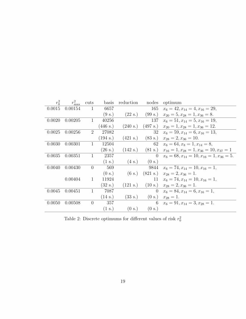
In Table 2 we show the results of the application of our algorithm assum-ing different risk levels. Each risk level is organized in a block of two rows.The first one gives the corresponding information, and below we report onthe elapsed time to obtain these elements. Column r2max contains the greatestrisk reached in the polytope with the number of added tangents as shown bythe following column. Column ‘basis’ denotes the number of elements of thecomputed test-set, and column ‘processed’ contains the number of new nodesfound and explored. Finally, column ‘optimum’ is a feasible point with the

18

r20 r2max cuts basis reduction nodes optimum0.0015 0.00154 1 6657 165 x6 = 42, x14 = 4, x16 = 29,

(9 s.) (22 s.) (99 s.) x20 = 5, x28 = 1, x36 = 8.0.0020 0.00205 1 40256 137 x6 = 51, x14 = 5, x16 = 19,

(446 s.) (240 s.) (497 s.) x20 = 1, x28 = 1, x36 = 12.0.0025 0.00256 2 27082 32 x6 = 59, x14 = 6, x16 = 13,

(194 s.) (421 s.) (83 s.) x28 = 2, x36 = 10.0.0030 0.00301 1 12504 62 x6 = 64, x8 = 1, x14 = 8,

(26 s.) (142 s.) (81 s.) x16 = 1, x28 = 1, x36 = 10, x37 = 10.0035 0.00351 1 2357 0 x6 = 68, x14 = 10, x16 = 1, x36 = 5.

(1 s.) (4 s.) (0 s.)0.0040 0.00430 0 569 9844 x6 = 74, x14 = 10, x16 = 1,

(0 s.) (6 s.) (821 s.) x28 = 2, x36 = 1.0.00404 1 11924 11 x6 = 74, x14 = 10, x16 = 1,

(32 s.) (121 s.) (10 s.) x28 = 2, x36 = 1.0.0045 0.00451 1 7087 0 x6 = 84, x14 = 6, x16 = 1,

(14 s.) (33 s.) (0 s.) x28 = 1.0.0050 0.00508 0 357 6 x6 = 91, x14 = 3, x28 = 1.

(1 s.) (0 s.) (0 s.)

Table 2: Discrete optimums for different values of risk r20

19

best return. The time in seconds of these tasks appears in parenthesis underthe columns ‘basis’, ‘reduction’ and ‘nodes’, respectively.

It is worth remarking the case r2 = 0.0040. The first row shows thenumber of processed nodes until an optimal point was reached, with no addedcutting hyperplane. The second row gives us an example of the effectivenessof adding new cuts. The test-set is computed very quickly, although thenumber of elements is big. However, the number of processed points is verysmall, and hence it is also small the total elapsed time.

r2max tang. basis reduction Sw1 Sw2 nodes improvement0.00118 3 32495 0 1 max

(244 s.) (333 s.) (426 s.)1 0 88 x6 = 35, x8 = 36, x14 = 2,

(176 s.) (0 s.) x16 = 27, x20 = 8, x28 = 31,x35 = 3, x36 = 3, x43 = 1

0.00107 4 16930 0 1 max x6 = 34, x8 = 22, x14 = 2,(52 s.) (130 s.) (393 s.) x16 = 29, x20 = 9, x28 = 24,

x35 = 3, x36 = 3, x43 = 1reached at 2894 nodes in 48 s.

0.00107 4 18637 0 1 max(49 s.) (114 s.) (439 s.)

1 0 9759 x6 = 33, x8 = 29, x14 = 2,(80 s.) (785 s.) x16 = 31, x20 = 9, x28 = 26,

x35 = 2, x36 = 30.00105 4 14670 0 1 max x6 = 34, x8 = 32, x14 = 2,

(28 s.) (79 s.) (627 s.) x16 = 29, x20 = 8, x28 = 10,x35 = 3, x36 = 4, x43 = 2reached at 1680 nodes in 29 s.

0.00101 2 2613 0 0 2648 x6 = 34, x8 = 32, x14 = 2,(1 s.) (10 s.) (853 s.) x16 = 29, x20 = 8, x28 = 10,

x35 = 3, x36 = 4, x43 = 2optimum

Table 3: Steps in the computation for r20 = 0.0010

Table 3 contains all the iterations done in the computation of the op-timum for the case r20 = 0.0010. The column Sw1 refers to the variableSwFictBounds, and Sw2 to SwNumNodes. The first one is true when

20

fictitious bounds are used, and the second one is true when the number ofprocessed records is greater than MaxNumNodes = 10000. The column‘improvement’ contains a new point found with better return than the initialpoint. Again, the time in seconds of each task appears in parenthesis.

Example 5.2. This example is devoted to show the difference between therounded continuous solution and the integer solution of a portfolio problem.It consists of a mixing of usual stocks (Microsoft and General Electric) withthe value of a future contract based on oil, as in [Chn09], so the number ofvalues is n = 3. The initial data is given by

Stock Price (ai) Return (µi)MSFT 35.22 3.64GE 36.76 3.64Oil 4000 10000

and the covariance matrix is

Ω =

0.003250634 0.000654331 0.0225132630.000654331 0.001578359 −0.0066108610.022513263 −0.006610861 26.35846804

.

We fix the risk to r20 = 1.52, and compute the optimum for differentbudgets B. The test-set associated with the constraints

atx ≤ B,Re ≤ µtx ≤ bRcc,x ∈ (Z+)n

has 2663 elements. The basis remains equal for all the considered cases.However, the capacity of computation is run out when only one more cutis added. If we take as initial point pe, the discrete approximation givenby rounding, the tree searching was unable to reach the optimal point forMaxNumNodes = 50000. This fact is reported as ‘E’ in Table 4

The function ComputeDiscreteApprox should be changed to get a betterdiscrete approximation than the rounded value. If we take an approximationbased on the best value for the future contract, we get Table 4.

It is easy to see the enormous difference between the return of the discreteapproximation and the corresponding return of the discrete optimum for eachbudget.

21

continuousBudget optimum return nodes optimum Rd

50000 (1079.87, 0, 2.99) 33848.34discrete approx.

(1192, 0, 2) 24338.88 E(219, 824, 3) 33796.52 6066 (314, 705, 3) 33815.06

75000 (1619.80, 0, 4.49) 50772.52discrete approx.

(1675, 0, 4) 46097.00 22790 (1675, 0, 4) 46097.00100000 (2159.74, 0, 5.98) 67696.69

discrete approx.

(2271, 0, 5) 58266.44 E(439, 1646, 6) 67596.69 22991 (687, 1409, 6) 67629.44

Table 4: Mixed example

6 Conclusions

We have presented an algorithm to deal with portfolio problems with integervariables and non-linear constraints. The presented model was not previouslytreated as far as we know. The method is based on the computation of sometest sets using Grobner bases, an algebraic tool. These Grobner bases arecomputed from a linear integer subproblem that contains the original linearconstraints and some new cuts induced by the non linear constraints. Thereversal test-set, given by the Grobner basis, allows us to perform a dualsearch algorithm from the optimal solution of the linear subproblem towardsthe optimal solution of the whole portfolio problem. This technique hasallowed us to solve problems of size similar to the exposed in [CF07, LT08].

Acknowledgments

This research was supported by grants P06-FQM-01366 and FQM-333 (Juntade Andalucıa), MTM2007-64509 and MTM2007-67433-C02-01 (Ministeriode Educacion y Ciencia). We wish to thank Javier Nogales for beneficialdiscussions.

22

References

[AL94] William W. Adams and Philippe Loustaunau. An introductionto Grobner bases, volume 3 of Graduate Studies in Mathematics.American Mathematical Society, Providence, RI, 1994.

[Bie96] Daniel Bienstock. Computational study of a family of mixed-integer quadratic programming problems. Mathematical Program-ming, 74(2, Ser. A):121–140, 1996.

[BL07] P. Bonami and M.A. Lejeune. An exact solution approach forportfolio optimization problems under stochastic and integer con-straints. IBM Research Report RC24215 (W0703-049), IBM Re-search Division, Thomas J. Watson Research Center, March 2007.

[BPT00] D. Bertsimas, G. Perakis, and S. Tayur. A new algebraic geom-etry algorithm for integer programming. Management Science,46(7):999–1008, 2000.

[BW05] D. Bertsimas and R. Weismantel. Optimization over Integers.Dynamic Ideas, 2005.

[CF07] M. Corazza and D. Favaretto. On the existence of solutions to thequadratic mixed-integer mean-variance portfolio selection prob-lem. European Journal of Operational Research, 176(3):1947–1960, 2007.

[Chn09] Michael T. Chng. Economic linkages across commodity futures:Hedging and trading implications. Journal of Banking & Finance,33:958–970, 2009.

[CLO05] David A. Cox, John Little, and Donal O’Shea. Using algebraic ge-ometry, volume 185 of Graduate Texts in Mathematics. Springer,New York, second edition, 2005.

[CT91] Pasqualina Conti and Carlo Traverso. Buchberger algorithm andinteger programming. In Applied algebra, algebraic algorithmsand error-correcting codes (New Orleans, LA, 1991), volume 539of Lecture Notes in Comput. Sci., pages 130–139. Springer, Berlin,1991.

23

[Dye92] Martin E. Dyer. A class of convex programs with applications tocomputational geometry. In Symposium on Computational Ge-ometry, pages 9–15, 1992.

[GK87] Monique Guignard and Siwhan Kim. Lagrangean decomposition:a model yielding stronger Lagrangean bounds. Mathematical Pro-gramming, 39(2):215–228, 1987.

[GK08] H. Geman and C. Kharoubi. WTI crude oil futures in portfoliodiversification: The time-to-maturity effect. Journal of Bankingand Finance, 32(12):2553–2559, December 2008.

[JHLM01] N. J. Jobst, M. D. Horniman, C. A. Lucas, and G. Mitra. Com-putational aspects of alternative portfolio selection models in thepresence of discrete asset choice constraints. Quantitative Fi-nance, 1(5):489–501, 2001.

[KTH79] M. K. Kozlov, S. P. Tarasov, and L. G. Hacijan. Polynomialsolvability of convex quadratic programming. Dokl. Akad. NaukSSSR, 248(5):1049–1051, 1979. Translated in Sov. Math., Dokl.20, 1108-1111 (1979).

[LC98] H.-L. Li and C.-T. Chang. An approximate approach of globaloptimization for polynomial programming problems. EuropeanJournal of Operational Research, 107(3):625–632, 1998.

[LT08] Han-Lin Li and Jung-Fa Tsai. A distributed computation algo-rithm for solving portfolio problems with integer variables. Euro-pean Journal of Operational Research, 186(2):882–891, 2008.

[Mar52] Harry M. Markowitz. Portfolio selection. Journal of Finance,7:77–91, 1952.

[Mar00] Harry M. Markowitz. Mean-variance analysis in portfolio choiceand capital markets. Wiley, New York, 2000.

[Mit03] H. D. Mittelmann. An independent benchmarking of SDP andSOCP solvers. Math. Program., 95(2, Ser. B):407–430, 2003. Com-putational semidefinite and second order cone programming: thestate of the art.

24

[MM91] Philippe Michelon and Nelson Maculan. Lagrangean decompo-sition for integer nonlinear programming with linear constraints.Mathematical Programming, 52(2, Ser. B):303–313, 1991.

[MM08] Richar O. Michaud and Robert O. Michaud. Efficient asset man-agement: a practical guide to stock portfolio optimization and as-set allocation. Oxford University Press, New York, 2008.

[Sha71] W. Sharpe. A linear programming approximation for the generalportfolio analysis. Journal of Finance and Quantitative Analysis,6:1263–1275, 1971.

[SM05] Bernd Scherer and R. Douglas Martin. Introduction to modernportfolio optimization with NUOPT and S-PLUS. Springer, NewYork, 2005.

[SNT85] Yoshikazu Sawaragi, Hirotaka Nakayama, and Tetsuzo Tanino.Theory of multiobjective optimization, volume 176 of Mathematicsin Science and Engineering. Academic Press Inc., Orlando, FL,1985.

[Sto73] B. Stone. A linear programming formulation of the general port-folio selection model. Journal of Financial and Quantitative Anal-ysis, 8:621–636, 1973.

[Stu96] Bernd Sturmfels. Grobner bases and convex polytopes, volume 8of University Lecture Series. American Mathematical Society,Providence, RI, 1996.

[tt08] 4ti2 team. 4ti2—a software package for algebraic, geomet-ric and combinatorial problems on linear spaces. Available atwww.4ti2.de, 2008.

[TTN95] Sridhar R. Tayur, Rekha R. Thomas, and N. R. Natraj. An al-gebraic geometry algorithm for scheduling in presence of setupsand correlated demands. Mathematical Programming, 69(3, Ser.A):369–401, 1995.

[YK91] H. Yamakozi and H. Konno. Mean absolute deviation portfoliooptimization model and its application to Tokyo stock market.Management Science, 37:519–531, 1991.

25

[You98] M.R. Young. A minimax portfolio selection rule with linear pro-gramming solution. Management Science, 5(44):637–683, 1998.

F. Castro Jimenez. Dpto. de Algebra, Univ. de Sevilla, Apdo. 1160, 41080Sevilla, e-mail: castro@us.es

J. Gago Vargas. Dpto. de Algebra, Univ. de Sevilla, Apdo. 1160, 41080Sevilla, e-mail: gago@us.es

I. Hartillo Hermoso. Dpto. de Matematica Aplicada I, Univ. de Sevilla,E.T.S. de Ingenierıa Informatica, Avda. de Reina Mercedes, s/n, 41012Sevilla, Spain, e-mail: hartillo@us.es

J. Puerto Albandoz, Dpto. de Estadıstica e Investigacion Operativa, Univ.de Sevilla, Facultad de Matematicas, C/ Tarfia, s/n, 41012 Sevilla, e-mail:puerto@us.es

J.M. Ucha Enrıquez. Dpto. de Algebra, Univ. de Sevilla, Apdo. 1160, 41080Sevilla, e-mail: ucha@us.es

26

Appendix

Procedure NewPolytope(polytope P , matrix Q, point pe, Tol, r0,MaxNumCuts)

NumCuts = 0 ;pmax, r

2m = ComputeMaxRisk(P,Q) ;

/* solve the problem maxQ(x),x ∈ P. */;while r2m − r20 > Tol and NumCuts ≤MaxNumCuts do

s = pe + λ(pmax − pe), λ ≥ 0 ;p′ = s ∩Q ;v = TangentToQuadric(Q,p′) ;DirApprox = Round(v, P rec) ;

/* round with number of digits = Prec */;Coef = TangentToQuadricV(DirApprox,Q) ;

/* independent term of the tangent hyperplane Q and

normal vector equal to DirApprox */ ;Coef = Ceil(Coef) ;

/* the best integer to leave the quadric in a

half-space */ ;H := DirApproxtx− Coef ;

/* new linear cut */ ;NumCuts = NumCuts+ 1;P = Polytope(P,H) ;

/* add a new cut to polytope P */ ;pmax, r

2m = ComputeMaxRisk(P,Q) ;

endreturn P

27

Algorithm 1: DiscreteOptimum

Data: budget B, risk r20, matrix Q, vector a, vector µ,MaxNumCuts, MaxNumNodes, Tol

Result: Optimum, NumNodesProcpc = ComputeContinuousOptimum(B, r20, Q,a,µ), gc = µtpc, α = 1/2 ;pe, ge = ComputeDiscreteApprox(pc, B,a, r

20, Q) ;

SwEOP = false, SwFictBounds = false, SwImprove =false, SwNumNodes = false, ListOfV ariables = (1 : dim) ;while not SwEOP do

if not SwFictBounds thenb, ListOfV ariables =ComputeLowerBounds(ListOfV ariables,pe) ;

endP = Polytope(atx ≤ B,µtx ≤ gc,µ

tx ≥ gd,x ≥ b) ;NumNodesProc = 0 ;while not ( SwEOP or SwImprove or SwNumNodes) do

P = NewPolytope(P,Q,pe, T ol, r0,MaxNumCuts) ;G = ComputeTestSet(P ),pini = Reduce(pbounds, G) ;SwNumNodes, SwImprove,Optimum =TreeSearch(pini, G,Q,a, B, r

20, b,pe,MaxNumNodes, SwFictBounds)

;if SwFictBounds then

if not SwImprove thenSwEOP = true ;

elsepe = Optimum, ge = µtOptimum, SwFictBounds =false ;

end

elseif not SwNumNodes then

SwEOP = true ;else

if not SwImprove thenb = b+ α(pe − b), SwFictBounds = true ;

end

end

end

end

end28