AN ALGEBRAIC APPROACH TO COMPILER DESIGN

AN ALGEBRAIC APPROACH TO COMPILER DESIGN

by

Augusto Sampaio

Technical Monograph PRG-110 ISBN 0 902928 872

October 1993

~ Oxford University Computing Laboratory Programming Research Group Wolfson Building Parks Road Oxford OXl 3QD England

Oxford lJnIV8rSitY ()lmpUtil1ll Laboratory WoIrsan BuiIlIl1lI

PllbRoacl bd OX1IQD

--

Copyright copy 1993 Augusto Sampaio

Oxford University Computing Laboratory Programming Research Group Wolfson Building Parke Road Oxfmd OXl 3QD England

shy

~

An Algebraic Approach to

Compiler Design

Augusto Sarnpaio

Wolfson College

J

A thesis submitted for the degree of Doctor of Philosophy at the University 0 Ozord Trinity Term 1999

Abstract

The general purpose of this thesis is to inve8tigate the design of compilers for procedushyrallanguagea based on the algebraic laws which these languages satisfy The particular strategy adopted is to reduce an arbitrary source progrQlIl to a nonna form which deshyscribes precisely the behaviour of the target machine This is achieved by a series of algebraic transformations which are proved from the more basic laws The correctness of the oompiler follows from the correctness of each algebraic transformation

The entire process is formalised within this single and uniform semantic framework of a procedural language and its algebraic laws But in order to attain abstraction and more reasoning power the language comprises specification features in addition to the programming constructs to be implemented These features are used to define a very general normal fonn capable of representing an arbitrary target machine The normal form reduction theorems can therefore be reused in the design of compilers which produce code for distinct target machines

A central notion is an ordering relation on programs p r q means that q is at least as good as p in the sense that it will meet every purpose and satisfy every specification satisfied by p Furthermore substitution of q for p in any context is an improvement (or at least will leave things unchanged when q is semantically equivalent to p) The compiling task is thereby simplified to finding a normal form that is not just the same but is allowed to be better than the original source code Moreover at all intermediate stages we can postpone details of implementation until the most appropriate time to make the relevant design decisions

Dijkstras guarded conuDand language is used to illustrate how a complete compiler can be developed up to the level of instructions for a simple target machine Each feature of the language is dealt with by a separate reduction theorem which is the basis for the modularity of the approach We then show how more elaborate features such as procedures and recur5ion can be handled in complete isolation from the simpler features of the language Although the emphasis is on the compilation of control strudures we develop a scheme for compiling arrays This is also an incremental extension in the sense that it has no effect on the features already implemented

A large subset of the theory is mechanised as a collection of algebraic structures in the OBJ3 term rewriting system The reduction theoreIllB are used as rewrite rolell to carry out compilation automatically The overall structure of the original theory is preserved in the mechanisation This is largely due to the powerful module system of OBJ3

Acknowledgements

I wish to thank my supervisor Prof CAR Hoare whose constant teaching advice and encouragement have helped me greatly He has originated the approach to compilation which is investigated here and has suggested the project which gave rise to this thesis

No lesa help I had from He Jifeng who made himself always available and acted as my second supervisor Most of what is reported in chapters 3 and 4 resulted from joint work with Prof Hoare and He Jifeng

My examiners Prof Mathai Joseph and Bernard SuIrio contributed comments suggesshytiODS and corrections which helped to lmprove this thesis

The work of Ralph Back Carroll Morgan Joseph Morris and Greg Nelson has been a great source of inspiration

Many thanks are due to the Declarative group led by Prof Joseph Goguen Apart from OBJ I have learned much about algebra and theorem proving attending their group meetings The diSCU88iow about OBJ with Adolfo Socorro Paulo Borba Grant Malcolm and Andrew Stevens were extremely helpful for the mechanisation reported in Chapter 6

I thank David Naumann Adolfo Socorro and Ignacio Trejos for pointing out errors and obscuritie8 in an early draft of this thesis and for many useful corrunents aDd suggesshytions I am also grateful to Ignacio mjos for constantly drawing my attention wrelevant bibliography and for the discussions about compilation and the refinement calculus

My former Msc supervisor Silvio Meira introduced me to the field of formal methods I thank him for the permanent encouragement and for influencing me to come to Oxford

I am grateful to my coUeague8 in the Attic for making it a pleasant working environment especially to Nacho for his company during the many nights we have spent there and to Gavin for his patience to answer so many questions about English

I tbank people at the Wolfson College for their support and friendship especially to the IleIDOr tutors (John Penney and Roger Hall) for help with the Day Nurllery fees

Some very good friends have been responsible for the best moments I have had in England Special thanks go to Adolfo Tetete Nacho George Hennano Max and Robin amp Chris I also thank Adolfo and Tetete (or the baby-sitting

I thank my parents my parents-in~lawmy brothers my sisters-inmiddotlaw and Daia for their continued support which can never be fully acknowledged The weekly letters from my mother made me feel not 80 far away from home

The roost special thanks go to Claudia (or aU the encouragement dedication and pashytience but above aU for providing me with the most essential ingredient of life-bye My little daughter Gabi has constantly distracted me from work demanding the attention of another full-time job--but one of enjoyment and happiness which brought lots of meaning into my life

Financia18upport for this work was provided by the Brazilian Research Council CNPq

Contents

1 Introduction 1

11 The Approalth 3

12 Overview of Subsequent Chapters 6

2 Background 8

21 PILCtial Orders and Lattices 9

22 The LaLtice of Predicates 10

23 The Lattice of Predicate Transformers 10

24 Properties of Predicate Transformers II

25 Some Refinement Calculi 12

26 Data Refinement 13

27 Refinement and Compilation 16

3 The Reasoning Language 18

31 Concepts and Notatioo 19

32 Skip Abort and Miracle 21

33 Sequential Composition 21

34 Demonic Nondeterminism 22

35 Angelic Nondeterminisffi 23

36 The Ordering Relation 23

37 Unbounded Nondetermlni5ID 24

38 Reltursion 26

39 Approximate In~rses 26

310 Simulation 28

311 ABBUIDption and Assertion 30

Contents ii

312 Guarded Command 31

313 Guarded Command Set 32

314 Conditional 33

315 Assignment - 34

316 Generalised Assignment 35

317 Iteration 37

318 Static Declaration 40

319 Dynamic Declaration 43

320 The Correctness of the Basic Laws 47

4 A Simple Compiler 40

4l The Normal Form 50

42 Normal Form Reduction 51

43 The Target Machine 56

44 Simplification of Expressions 57

45 Control Elimination 60

46 Data Re1inement 63

47 The Compilation Process 68

5 Procedures Recursion and Parameters 71

51 Notation 71

2 Procedures 73

53 Recursion 15

54 Parameterised Programs 78

55 Parameterised Procedures 82

56 Parameterised Recursion 83

57 Discussion 84

6 Machine Support 86

61 OBJ3 87

62 Structure of the Specification 89


631 An Example of a Proof 95

64 The NoTJDA1 Fonn 97

65 A Compiler Prototype 98



653 Data Refinement 10)

654 Machine Instructions middot 101

655 Compiling with Theorems middot 102

66 Final Considerations middot 104

661 The Mechanisation middot 105

662 OBJ3 and 20BJ 106

663 Other systems middot 108

7 Conclusions 110

71 Related Work middot 112

72 Future Work middot 115

73 A Critical View middot 121

Bibliography U2

A A Scheme for Compiling Arrays 128

B Proof of Lemma 51 131

C Specification and Verification in OBJ3 135

CI The Reasoning Language 135

Cl1 Proof of Theorem 3176 139

C12 Proof of Theorem 3177 141

C2 The Normal Form 144

C21 Proof of Lemma 42 145



C3 Simplification of Expressions 148



Contents v

C4 Control Elimination

CS Data Refinement

CS1 Proof of Theorem 410

C52 Proof of Theorem 414

C6 Machine Instructions

middot 151

middot 152

middot 152

middot 154

middot 157

Chapter 1

Introduction

We must not lose sight of the ultimate g~l Iflat of the construction of programming language implementations which are known to be correct by virtue of t~ quality of the logical reasoning which ~5 been devoted to them Of course such an imp~mentation will still rJeed to be comprehensively tested before delivery but it will imshymediately pass all the tests and then continlll to WCMk correctly for the bene6t of programmers flaquoever after

- CAR Hoare

The development of reliable systems bas been one of the main challenges to computing scientists This is a consequence of the complexity of the development procas which UBUally comprises many stagel from the original capture of requirements to the hardware in which programs will TUn

Many theoriel methods techniques and toola have been developed to deal with adjacent stages For example the derivatioD oC progt8Jll8 from specifications the translation of proshygrams into machine code (compilation) and 90metimes even a gate-level implementation of the hardware Nevertheless the development of a mathematical model to ensure global consistency of the process in general has attracted very little attention most certainly because of the intricacy of the task

Perhaps the most significant effort in this direction is the work of a group at Compumiddot tational Logic Inc [7] They suggest an operational approach to the development and mechanical verification of systems The approach has been applied to many Sj51em comshyponents including a oompiler alinkmiddotassembler and a gate-level design of a microprocessor The approach is independent of any particular component and deAls with the fundamental aspect of integration of components to form a verified stack

This work inspired amp European effort which gave rise to the Esprit project Provably Correct System (PraCaS) [9 12] This project also aims to cover the entire development process The emphasis is on a constructive approach to correctness using provably correct transformations between all the phases It differs IDQ9tly from the previously cited work in

2 IntrodUdion

that an abstract (rather than operational) Universal model is being developed to ensure consistency ampcr088 all the interfaces between the development phases Furthermore a more ambitioWl scope is attempted including explicit parallelism and time constraints throughout the development The reusability of designs and proofs is also an objective of the project

Our work is in the context of PraCoS We are concerned with the compilation phase the translation of programs to machine code But the emphasis is on an algebraic approach to compilation rather than in the translation between a particular pair of languages Although neither the source language nor the target machine we use as examples coincide with the ones of tbe ProCoS project it is hoped that the overall strategy suggested here will be useful to design the compiler required in the project and many others

A large number of approaches have been suggested to tackJe the problem of compiler correctness They differ both in the semantic style adopted to define source and target languages (operational denotational algebraic axiomatic attribute grammars ) and in the meaning of correctness associated with the translation process The first attempt was undertaken by McCarthy and Painter [52J they used operational semantics to prove the correctness of a compiler for a simple expression language The algebraic approach originate with the work of Burstall and Landin 14] Both works have been of great impact and many researchers have built upon them A brief suIIlIIlUY of some of the main approaches to compiler correctness is included in the final chapter

Hete we further develop the approach introduced in [45] where compilation is identified with the reduction of programa (written in a procedural language) to a normal form which decribes precisely the behaviour of the target executing mechanism The reduction process entails a series of semantic-preserving transformationsj these are proved from more basic laws (ampXiOIllB) which give an algebraic semantiC8 to the language

A central notion is an ordering relation on programplIlB p ~ q means that q is at least as good as p in the sense that it will meet every purpose and satisfy every specification satisfied by p Furthermore substitution of q for p in any context is an improvement (or at least will leave things unchanged when q is semantically equivalent to pl The compiling task is thereby simplified to finding a nonnal form that is Dot just the same but is alJowed to be better than the original source code Moroover at all intermediate stages we can postpone details of implementation until the most appropriate time to make the relevant design decisions

Another essential feature of the approach is the embedding of the programming language into a more general space of specifications This includes constructions to model features such as assumptions and aBsertions and even the less familiar concept of a mirocle standshying for an unsatisfiable speltmcation The specification space forms a complete distributive lattice which allows us to define approximate inverses (Galois connections) for programmiddot ming operators The purpose of all of this is to achieve a very abstract normal form definition (which can model an arbitrary executing mechanism) and 8imple and elegant proofs We hope to prove this claim

bull A blief overview of the lattice theory relevant Lo us is ~ven in tbe De1t chapter

All the calculations necessary to aBeerl the correctnetls of the compilation process are carshyried out within this single framework of a specification language whose eemantics is given by algebraic laws No addjtional mathernatiLA1 theory of BOurce or target language is deshyveloped or ~ in the process The relatively simple reasoning framework its abstraction ana moaularity are the main features of the approach

We select a small programming language (including iteration) to illustrate how a complete compilerl can he developed up to the level of instructions for an abstract machine Each feature of the language is dealt with by a separate reduction theorem which is tbe basis for the modularity of the approach We then show how more elaborate features such all

procedures and recursion can be handled in complete isolation from the simpler features of the language

A large subset of the theory is mechanisea as a collection of algebraic structures in the OBJ3 [31] term rewriting system The reduction theoreTrul are used aB rewrite rules to carr) out compilation automatically The overall structure of the origina11hoory is preserved in the mechanisation This is largely due to the powerful module system of 08J3

11 The Approach

In this section we give an overview of our approach to compilation based on a simple example We also identify the scope of the thesis in terms of the sowce language that we deal with the additional specification featurea and the target machine used to illustrate an application of the approach

The BOWce progranuning language contains the following constructions

skip do nothing

= e assignment

pj q sequential composition

pnq nondeterminism (demonic)

p4 btgtq conditional if b then p else q

b p iteration while b ao p

dec z bull P (static) declaration of variable z for use in program p

PfOCX=pq procedure X with hody p and scope q

jJ X bull p recUI6ive program X with body p

We avoid defining a syntax for expressionsj we use uop and bop to stand for arbitrary unary and binary operators reapectively Initially we deal with a simplified version of the

2We addre8ll 001) tbe code generation phase of a compiler Paning and ampemantic analyBis are not dalt lfitb Optimisaiion ill hrieB) cODSidred alI a topic for future resetIIcb

11 The Approach 4

language not including procedures or recursion These are treated later together with the issue of parameterisation

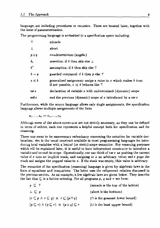
The programming language is embedded in a specification space including

T miracle

1- abort

pUq nondetenninism (angelic)

I assertion if b then skip else l

IT assumption if b then slOp else T

Ip guarded conunand if b then p ehle T

~E b generalised assignment aasign a value to x which makllS b true if not possible x E b behaves like T

var x dedac8otion of vari80ble x with undetermined (dynamic) scope

end x end the previous (dynamic) scope of x introduced by a var x

Furthermore while the source langu8oge allows only single assignments the specification language allows multiple assignments of the form

Xl bullbull bull x = el e

Although some of the above constructs are not strictly necessarYI as they can be defined in terms of others each One represents a helpful concept both for specification and for reasoning

There may seem to he unnecessary redundancy concerning the not8otion for vari80ble decshylarations dec is the usual construct available in most progr8omming languages for introshyducing local variables with a lexicaJ (or static) scope semantiCfl For reasoning purposes which will be explained later it is useful to have independent constructs to introduce a variable and to end its scope Operationally one can think of val x as pushing the current value of x into an implicit stack and assigning to x an arbitrary vallle end ~ pops the stack and assigns the popped value to x If the stack was empty this value is arbitrary

The semantics of the specification (reasoning) language is given by algebraic laws in the form of equations and inequations The latter uses the refinement relation discussed in the previous section As an example a few algebraic l8ow8 are given below They describe the fact that is a lattice ordering For all programs p q and r we hayenc

p T (miracle is the top of the lattice)

1shy [ P (8ooort is the bottom)

([pA [q) [(pnq) (n is the greatest lower bound)

(p[)A(q[) (pUq)[ (U is the least upper bound)

We define a simple target machine to illustrate the design of a compiler It consists of four components

P a sequential register (program counter) A a general purpose register M a store for variables (RAM) m a store for instructions (ROM)

The instructions can be designed in the usual way as assignments tbat update the machine state for example

Ied(n) l AP=M[n]P+l

store(n) dj M P= (M Ell (n ~ AJ)P + 1

where we use map overriding (EEl) to update M at position n with the value of A The more conventional notation is M[n] = A

The normal form describing the behaviour of this machine (executing a stored program) is an iterated execution of instructions taken from the store m at location P

deeP A bull P= s (s S P ltf) m[PJ (P =fh

where s is the intended start address and f the finish address of the code to be executed The obligation to start at the right instruetion is expressed by the initial assignment P = 5 and the obligation to terminate at the right place (and not by a wild jump) is expressed by the final assertion (P = fh The design of a compiler is nothing but a construetive proof that every program however deeply structured can be improved by some program in this normal form The process is split into three main phases concerns of control elimination are separated from those of expression decomposition and data representation In order to illustrate theuroSe phases consider the compilation of an assignment of the form

x= y

where hoth x and y are variables The simplification of expressions must produce assignshyments which will eventually give rise to one of the patterns used to define the machine instruetions Recalling that A represents the general purpose register of our simple mashychine this assignment is transformed into

decA bull A= y x = A

where the first assignment will become a load and the second one a store instrudion But this program still operates on abstract global variables with symbolic names whereas the target program operates only on the concrete store M We therefore define a data refineshyment W which maps each program variable r onto the corresponding machine location so the value of x is held as M[Wx] Here 11 is the compilers symbol table an injection which maps each variable onto the distinct location allocated to hold its value Therefore


we need a data refinement pbase to justify the substitution of M[x] for x tbroughout the program Wben this data refinement is perfonned on our simple example program it becomes

dA A = M[pyJ M = M III p ~ A

The remaining task of the compiler is that of control refinement reducing the nested control structure of tbe source program to a single flat iteration like tbat of the target program This is done by introducing a control state variable to schedule tbe selection and sequencing of actions fn the case of our simple target macbine a single program pointer P indicates the location in memory of tbe next instruction Tbe above then becomes

decPAP=s ) (P = ) ~ AP = M[py]P + 1

(SPltH2)middot(o (P=+l)~MP=(MEIgt~~A)P+l (P~+2h

where we use 0 as syntactic sugar for n when tbe choice is deterministic The initial assignrneDt P= s ensures that the assignment with guard (P = 8) will be executed first as this increments P the assignment with guard (P = s + 1) is executed next This also increments P falsifying the condition of the iteration and satisfying the final assertion

Note that the guarded assignments correspond preci~ly to the patterns used to define the load and store instructions respectively The above expresses the fact that these instructions must be loaded into the memory m at positions 8 and s + I completing the overall process

The reduction theoreIrul which justify the entire process are al1 provably correct from the basic algebraic laws of the language Furthermore some of the proof are verified using OBJ3 and the reduction theorems are used M rewrite rules to do the compilation automatically

12 Overview of Subsequent Chapters

Chapter 2 describes in some detail the view of specifications as monotonic predicate transformers in the sense advocated by Dijkstra We review the mathematical concepts of partial orders and lattices and show that the language introduced above forms a complete distributive lattice of monotonic predicate transformers We give examples of refinement calculi based on these ideas and address the problem of data refinement Finally we link our approach to compilation to the more general task of deriving programs from specifications

In Chapter 3 we give meaning to the reasoning language in terms of equations and inshyequations which we call algebraic laws The final section of this chapter discusses how the laws can be proved by linking the algehraic semantics to a given mathematical model for the purpose of illustration we use weakest preconditions

A complete compiler for the simplified source language (that is not including procedures or recursion) is given in Chapter 4 The first two sections deBcrihe tbe normal form as a model of an arhi trary executing mechanism The reduction theorems associated with this form are largely independent of a particular way of representing control state We show that the use of a program pointer is one possible instantiation The design of the compiler is split into three phases as illustrated in Section 1l

In Chapter 5 we deal with procedures and recursion and address the issue of parametershyisation We sbow how each of these can be eliminated through reduction to normal form but we leave open the choice of a target machine to implement them Each feature is treated by a separate theorem in complete independence from the constructions of the simpler language This illustrates the modularity of the approach

Chapter 6 is concerned with the mechanisation of the approach The purpose is to show how this can be achieved using the OBJ3 term rewriting system There are three main activities involved The formalisation (specification) of concepts such as the reasoning language its algebraic laws the normal form the target machine and so on as acollection of theories in OBJ3 the verification of the related theorems and the use of the reduction theorems as a compiler prototype The final section of this chapter includes a critical view of the mechanisation and considers how other systems can be used to perform the same (or a similar) task

In the final chapter we sununarise our work and discuss related and future work The very final section contains a brief analysis of the overall work

Apart from the main chapters there are three appendices Although the emphasis of our work is on the compilation of control structures Appendix A describes a scheme for compiling arrays Appendix B contains the proof of a lemma used to prove the reducshytion theorem for recursion Appendix C contains more details ahout the mechanisation including complete proofs of some of the main theorems

Chapter 2

Background

The beauty of lattice theory derives in part from the ell~

treme simplicity of its basic concepti (partial) ordering least UPP- and greatest lower bounds

- G Birkhoff

The pwpose of this chapter is to briefly describe a theoretical basis for the kind of reshyfinement amp1gebra we will be u8ing Based on the work of Morris [591 and Back and von Wright [5J we show that a specification language (as introduced in the previous chapshyter) forms a complete distributive lattice where foUowing Dijkstra [21] specifications are viewed as monotonic predicate transformers We give examples of refinement calculi based 00 these ideM and address the problem of data refinement Finally we Link ow approach to compilation to the more general task of deriving prograJD9 from 8pecifications

The first section review8 the concepts of partial orders and complete distributive lattices and a simple boolean lattice is presented as an example The next section describes the predicate lattice as functions from (program) states to booleans this is constructed by pointwise extension from the boolean lattice Further pointwise extension is used to construct the lattice of predicate transformen described in Section 23 theBe are functions from predicates to predicates In Section 24 we review some properties of predicate transformers (known as healthine1J8 conditions) and explain that some of them are dropped as a coMequence of adding non-implementable features to the language Some refinement calculi baaed on the predicate trampDBformer model are considered in Section 25 and some approaches to data refinement in Section 26 The final section relates all these to our work

8

21 Partial Orders and Lattices

A partial order is a pair (S) where S is a set and ~ is a binary relation (the partial ordering) on S satisfying the following axioms (or aU X y z E S

[ reflexivity (z ~ y) 1 (y ~ z) =gt (z ~ z) tranitivity (z ~ y) 1 (y ~ z) =gt (z = y) antiymmetry

(SI) is called a total order if in addition to the above each pair of elements in S are comparable (x [ y) V (y x) Following usual praclice we will abbreviate (S) to S the context will make it clear jf we are regarding S as a set or as a partial order

Given a subset T of S we say that rES is AD upper oound for T if y r z for all YET z is the least upper bound of T if it is both an upper hound for T and whenever y is another upper bound for T then z r y Similarly z is a lower bound for T if z ~ y for all YET z is the greate8t lower bound of T if it is hath a lower bound for T and whenever y is another lower bound for T then y z An element 1 is a least element or bottom of 5 if 1 z for all x E 8 T is a greate8t element or top of 5 if z T for all z E5

Given sets 8 ampnd T with T partially ordered hy T the set 8 - T of functions from S to T is partially ordered by defined by

f~g ~ f(z)~Tg(z) forallzES

Additionally if 8 is partially ordered by s tben f 8 - T is said to be monotonic jf

z~sy =gt f(z)~Tf(y) forallzyES

We denote by [8 _ TJ the set of monotonic functions from 5 to T H 8 is discrete (that is z ~s y holds if and only if z = y) then 8 - T and [5 - T] are identical

A complete lattice is a partially ordered set containing arhitrary greatest lower bounds (meets) and least upper bounds (joins) A consequence is that every complete lattice has a hottom and a top element Two additional well-known properties of complete latticea are given below more details about lattice theory caD be found for example in [8]

bull Any finite totally ordered set is a complete lattice

bull If S is a partially ordered set and T is a complete lattice then [8 _ T] is a complete lattice

A lattice is said to be distributive if the least upper bound operator distribute through tbe greatest lower bound operator I and vice versa

A very simple example of a complete distributive lattice is the boolean set trueJalse when ordered by the implication relation Tbe least upper bound V and the greatest lower bound bave their usual interpretations as disjunction and oonjunetion respectively The bottom element is fal8e and tbe top element is true This is actually a complete boolean lattice since it has a complement (negation) but we will not use tbis property In the next section we will refer to this lattice as Bool

22 The LaWre of Predicates 10

22 The Lattice of Predicates

Programs usually operate on a state space formed from a set of variables We use State to stand for the set of all p088ible states partially ordered by the equality relation therefore it is a discrete partial order In practice we need a way to describe particular sets of states for example to specify the set of initial states of a program as well as the set of its final states This can be described by boolean-valued functions (or predicates) on the state space

As State is a partial order and Baal is a complete lattice [State -+ Bool] is also a complete lattice Furthermore as State is discrete [State - Boo~ and State _ Bool are identical We will refer to it as the Predicate lattice The least upper bound a V b is the disjunction of the predicates a and b and the greatest lower bound a 1 b is their conjunction The bottom element false describes the empty set of states and the top element true describes the set of all possible states These operations are defined by

( V6) 1 gtz bullbull() V 6() ~I(6) = gt bullbullbull()6()

lrue ~ gt bull true

false JgJ gt bull false

where the bounded variable ranges over State The lattice ordering 1S the implication on predicates which is defined by pointwise extension in the usual way

bull =gt 6 1 IIbullbull a() =gt 6()

23 The Lattice of Predicate Transformers

The lattice presented next provides a theoretical basis for Dijkstras view of programs aB

predicate transformers (functions from predicates to predicates) [21] The usual notation

wp(p a) = c

means that if program p is executed in an initial state satisfying its weakeat precondition C1 it will eventually terminate in a state satisfying the postcondition a Furthermore aB

the name suggests the weakest precondition c describes the largest possible set of initial states which enBures that execution of p will terminate in a state SAtillfying a

The predicate transformer lattice (Predlhm) is the set of all monotonic functionll from one predicate lattice to another IPredicate - Predicate] The result of applying program (prediute transfonner) p to predicate a denoted p(a) ill equivalent to Dijkstras wp(p a) The ordering on predicate lransfonnerll ill defined by pointwise extension from the ordering on predicates

pq 1 lIap(a)=gtq(a)

24 Properties of Predicate Transformers 11

where the bounded variable a ranges over the set of predicatea

Clearly PredTron is a complete lattice and therefore it contains arbitrary least upper bounds and greatest lower bounds n is interpreted as demonic nondeterminism and U

as angelic nondeterminism The bottom element is abort (denoted by i) the predishycate transformer that does not estahlish any postcondition The tQp element is miracle (denoted by T) it establishes every postcondition These are defined in the obvious way

(pU q) 1 Aaop(a)Vq(a)

(pnq) 1 A a 0 p(a) 1 q(a)

T iJ Aa true

1- iJ A a bull false

The usual program constructs can be defined as predicate transformers As an example we define skip (the identity predicate transformer) and sequential composition

skip Aa bull a

pq 1 Aaop(q(a))

24 Properties of Predicate Transformers

Dijkstra 2l] has suggested five healthiness conditions that every construct of a proshygramming language mmt satisfy They are defined below (we assume implicit universal quantification over a and b standing for predicates and over p standing for programs)

I p(lI) = fl law of the excluded miracle 2 If a 0 then pIa) pro) monotoILicity 3p(a)p(o) = p(ao) conjunctivity 4p(a)Vp(o) = p(aVo) disjunctivity 5p(3ii~Oa) = 3ii~Op(a) continuity

for all sequences of predicates Go (11 bullbullbull

such that O-i ~ a+1 for all i ~ 0

The fourtb property is sati5fied only by deterministic programs for nondeterministic pro-shygraIIl8 the equality bas to be replaced by an implication The last property is ~uivalent

to requiring that nondeterminism be bounded 1231middot

The complete lattice PredTran includes predicate transformers useful for specification purshyposes they are not implementable in general Of the above properties only monotonicity is satisfied by all the predicate transformers in PredTran T trivially breaks the law of the excluded miracle the fact that greatest lower bounds over arbitrary sets are allowed implies that the assumption of bounded nondeterminism (and therefore continuity) is not satisfied and angelic nondetenrunism violates the property of conjunctivity

Of course the healthinC3s conditions are still of fundamental importance they are the criteria for distinguishing the implementable from the non-implementable in II general space of specifications

25 SOIne Refinement Calculi 12

25 Some Refinement Calculi

Back 13 5) Morris [59] and Morgan [55 56J have developed refinement calculi based on weakest preconditions These calculi have the common purpose of formalising the well established stepwise refinement method poundOr the systematic construction of programs from high-level specifications 176 20

As originally proposed the stepwise refinement method is partly informal Although specshyifications and progriLnl8 ale formal ohjects the intermediate terms of a given derivation do not havea formal status The essence of all the refinement calculi cited above is to extend a given proltedurallanguage (in particular Dijkstras guarded command language) with additional features for specification For example let [a c] be a specification construct used to describe a program that when executed in a state satisfying a terminates in a state satisfying c This can he viewed as a predicate transformer in just the same way as the other operatoCl of the language Its definition is given by

[ac] 1 Hoall(c=gtb)

The extended language is thus a specification language and programs appear as a subclass of specificatioDS Progranuning is then viewed as constructing a seqnence of specifications the initial specification is in a high-level of abstraction (not usually irnplementable) and the final specification is an executahle program The derivation procesa is to gradually transforro specifications into programs The intermediate steps of the derivation will normally contain a mixture of specification and program constructs but these are forshymal objects too since specifications and programs are embedded in the same semantic framework

Derivation requires tbe notion of a refinement relation between specifications All the cited calculi use the same definition of the refinement relation which is precisely the ordering on the lattice of predicate transformers described above Two mathematical properties of thi8 ordering are of fundamental importance to model stepwise refinement Monotonicity of the language operators with respect to this ordering is necessary to allow a given specification to be replaced by a refinement of it in an arbitrary context this can only refine the overall context The other required property is transitivity as the derivalion process will normally entail a large number of steps it is necessary to enBure that the final product (that is the program) satisfies the original specification

Rules for introducing programming constructs from given specifications are the additional tools required in the process For example the following rules illustrate the introduction of skip and sequential composition

[a cJ skip if a ~ c [a cl ~ la b] [b cJ

There are also rules for manipulating specificatioDS for example weakening the preshycondition of a given specification or strengthening its postcondition (or botb) lead to a specification which refines the original one

[at Ct] [lI2t cll if at =gt 112 1 C] =gt Ct

Morris [59J Wall the first to give a lattice theoretic basis for the refmement calculus He extended Dijkstras guarded command language with predicate pairs (as illustrated above) and generaJ recursion Although he observed that the frCLIlleWork contains arbitrary least upper bounds and greatest lower bounds these have not been incorporaLed into his specification language

Back and von Wright [5J further explored the lattice approach and suggested a more powerful (infinitary) language which is complete in the sen8e that it can express every monotonic predicate transformer The only constructortl in their language cue the lattice operators n and U together with functional comp08ition (modelling sequential composishytion) From a very simple command language including thegte constructorll they define ordinary program constructs such as assignment conditionaJ and recursion Inverses of programs are defined and used to fonnaJise the Dotion of data refinement This is further discus8ed in the next section

Morgans calculus [56] is perhaps the most appealing to practising programmers His language includes procedures (possibly recursive and parameteri3ed) and even modules He definetl a large number of refinement laws and illustrates their application in a wide range of derivations The specification statement

[a c]

is another distinctive feature of his work Although it is similar to the notation uged

above it includes the notion of a frame x is a list of variables who8e values IlUy change The frame reduces the number of p08sible refinements from a given specificatiotl and is a way of making the designers intention clearer Furthermore the above construct is very general and can be specialised for many useful purposegt For example our generaliBed assignment command can be regarded as a special case of it

xE a = x [truea]

where the purpose is to establish a without changing any variablegt other than x Another example is an lI88umption of a meaning that a must be egttablished without changing any variable

aT = [truea]

26 Data Refinement

In the previous section we discussed how an abstract specification is transforrred into a program by progressively introducing control structuregtj this is known amp8 agordhmic or control refinement But this is only part of the process to obtain an implementation Specshyifications are wually stated in terms of mathematical data types like sets and relations and these are not normally available in proceduraJ programming languages Therefore the complementary step to control refinement is the transformation of the ahstract types into concrete types such as arrays and recorda which can be efficiently implemented Thia task is known as data refinement


The idea of data refinement was first introduced by Hoare [41] The basis of his approach is the UBe of an abstrQction junction to determine the ab6tract state that a given concrete state represents in addition the set of concrete states may be constrained by an invanant relation Since then many approaches have been suggested which build on these ideas The more recent approaches use a single relation to capture both the abstraction function and the invariant thus relcuang the assumption that the abstract state is functionally dependent on the concrete state

In connection with the refinement calculi considered in the previous section two very similar approaches have been suggesled by Morris [61] and Morgan and Gardiner [57] In both cases data refinement is characterised as a special case of algorithmic refinement between blocks A block of the form

decx Tx bull p

is used to represent the abstract program p operating on the variables x with type Tx SimilarlYl

decl Tx p

represents the concrete program p which operates on the variables x with type Tx The data refinement is captured by the inequation

(decx Tx p) i (dec x Tx bull p)

The general aim is to construct the concrete block by replacing the abstract local variables with the concrete ones in such a way that the overall effect of the abstract block is preserved In particular pi is constructed with the same structure as p in the sense that each command in pi is the translation of a corresponding coIIlIIlAnd in p according to a uniform rule

An essential ingredient to this strategy is an abstract invampriant I which links the abstract variables x to the concrete variables Z This is called the coupling invanant A new relation between programs is defined to express that program p (operating on variables x) is a data refinement of program p (operating on variables z) under coupling invariant I This is written p 516r pi and is formally defined by (considering programs as predicate transformers )

p$ssp l (3xIlp(a))=gtp(3xIlo) for all 0 not containing x

Broadly the antecedent requires that the initial values of the concrete variables couple to some set of abstract values for which the abstract program will succeed in establishing postcondition ai the con8Cquent requires that the concrete program yields new concrete values that alBo couple to an acceptahle abstract state

~ l(e(llll that our language is untyped t)Pe8 Ile eoosidered bere only (or the purpose of ~be praeot di8CU88i(ID

This definition is chosen for two main rea8OWl The first is that it guarantees the characshyterisation of data refinement given above that is

If (p 5Iz~ p) then (decz Tz p) (decz Tz e p)

The second reason is that it distributes through the program constructors thus allowshying data refinement to be carried out piecewise For example the distribution through sequential composition is given by

If (p 5Is~ p) and (q 5Is~ q) then (Pi q) SIss (p q)

Back and von Wright [5J suggest an approach which avoids the need to define a data refinement relation They use the algorithmic refinement relation not only to characteri~

data refinement but also to carry out the caiculatioWl The basic idea is to introduce an encoding program say W which computes abstract states from concrete states and a decoding program program say tP which computes concrete states from abstrad states Then for a given abstract program p the task is to find a concrete program p such that

w p tP ~ p

With the aid of specification features it is possible to give very high-level definitions for p and tP Using the same convention adopted above that z stands for the abstract variables z for the concrete variables and I for the coupling invariant p il defined by

del LW= varz zE I endz

It first introduces the abstract variables z and B81igns them values such that the invariant is satisfied and then removes the concrete variables from the data space The use of lshyas an annotation in the above generalised assignment command meaIl8 that it aborts if I cannot be establisbed Similarly we have the definition of tP

leI TtP = varz zE I endz

which introduces the concrete variahles z and assigns them values such that the invariant is satisfied and then removes the abstract variahles from the data space But in thi8 case the generalised assignment command re5ults in a miracle if I cannot he established (The above two kinds of generalised assignment commands were introduced only for the purpose of the present discu88ion Reca1I from the previous chapter that our language includes only the latter kind and henceforth we will use the previous notation z E b)

Note that having separate commands to introduce and end the scope of a variable i8 an essential feature to define tbe encoding and decoding programs the first introducetl z and ends the scope of z i the second introduces Zl and ends the scope of z

In this approacb data refinement can also he perfonned piecewise by proving distribushytivity properties such as

p (p q) ~ C (p p ~) (p q ~)

which illuatrates that both algorithmic and data refinement can be carried out within the framework of one common refinement relation


27 Refinement and Compilation

As explained in the previous chapter we regard compilation as a task of program reshyfinement 1D this sense we can eatablish some connections between our view of compiler design and the more general task of deriving programs from specifications (henceforth we will refer to the latter simply as derivationn) ln both caaes a programming language is extended with specification features so that a unifonn framework is built and the inshyterface between programs and specifications (when expressed by distinct formalisms) is avoided In particular our language is roughly the same as the one defined by Back and von Wright [5] except that we deal with procedures and parameterisation The first three sections of this chapter briefly explained how the language can be embedded in a complete distributive lattice of predicate transformers

In a derivation the idea is to start with an arbitrary specification and end with a program formed solely from constructs which can be executed by computer In our case the initial object is an arbitrary source program and the final product is its normal fonn But the tools used to achieve the goals in both caaes are of identical nature transformations leading to refinement in the sense already di6Cussed

Derivation entails two main tasks control and data refinement We also split the design of the compiler into these two main phases However while in a derivation control refinement is concerned with progressively introdUcing control structure in the specification we do the reverse process we reduce the neated control structure of a source program to the single flat iteration of the normal fonn program

Regarding data refinement the general idea is the same both in a derivation procelS and in designing a compiler to replMe abstract data types with concrete representations In particular we use the idea of encoding and decoding programs As discussed in the previous section this avoids the need to define a separate relation to carry out data refinement In our case an encoding program retrieves the abstract SpMe of the source program from the concrete state representing the store of the machine Con~rsely a decoding program maps the ahstract space to the concrete machine state In the next chapter the pair fanned by an encoding and the respective decoding program is formally defined as a Simulation It satisfies the distributivity properties illustrated above allowing data refinement to be carried out piecewise

But as should be expected there are SOme differences between designing a compiler in this way and the more general task of deriving progrMllil from specifications For example we are not interested in capturing requirements in general and therefore our language includO no construct to serve this purpose The closest to a specification statement we have in our language is the generaJiaed aB8ignment command Our use of it is to abstract from the way control state is encoded in a particular target machine

Another diJference is that we are mostly concerned with program traIUlformation We need a wide range of laws relating the operators of the language In particular we follow the approach suggested by Hoare and others [41 where the semantics of a language is characterised hy a set of equations and inequations (laws) relating the language operaton

The same approach has been used to define an algebraic semantics for occam [68] In our case the set of laws must be complete in that it should Mlow us to reduce an arbitrary program to normal fonn The framework we use is better characterised as a refinement algebra (rather than as a calculus)

Chapter 3

The Reasoning Language

If)ClU are raced by a difficulty or a controversy in science an ounce of algebra is worth OJ ton of verbal argument

- JBS Haldane

Here we give meaning to our specification (reaaoning) language in terms of equations and inequatioDII (laws) relating the operators of the language Following Hoare and othshyers [47 68] we present the laws as self-evident ampXioms normally preceded by an informal (operatiooal) jwlification Moreover it is not our aim to describe a complete set of laws in the logical sense although they ampre complete in that they will allow us to reduce an arbitrary source program to a normal (orm

It is possible to select a small subset of our language and define the additional operator8 in terIlll of the more basic ones This is shown in [45] where the only constructors are sequential composition U and n The additiooaJ operators are defined in terms of these and the primitive commands The laws of derived operators can then be proved from their definition and the laws of the basic operators

This is not our concern here our emphasis is on the algebraic laws which will be used in the process of designing a compiler However we do illustrate how a few operators can he defined from others In pacticulac iteration is defined as a special case of recursion and all the lawll about iteration are proved They deserve such llpecial attention becawe of their central role in the proofs of the normal form reduction theorems

We will not normally distinguish between programs and llpecificationll We will refer to both of them as programs Another remark is that programs have both a syntactic and a semantic existence On one hand we perform llyntactic operations on tbem lluch as suootitution On the other hand the algebraic laws relating language operators exshypress semantic properties Strictly we should distinguish between these two natures of programs But it is not convenient to do 90 and it will be clear from the context wbich view we are taking

The first section gives notational conventions and introduCE the concepts of substitution and free and bound identifiers Each of the subsequent sections describes tbe laws of

18

one or more language operators The concepts of a refinement relation approximate inverse (Galois connection) and simulation will be introduced when the need arises The final section describes alternative ways in which the laws of the basic operators could be verified As an example we take the view of programs as predicate transformers (as discUBSed in the previous chapter) and illustrate how the laws can be proved

31 Concepts and Notation

Name conventions

It is helpful to define some conventions as regards the namell used to denote program terms

x YZ program identifiers pqr programs z YZ lists of variables abc boolean expressions eg lists of expressions

We also use subscripts in addition to the above conventions For example flo bt stand for boolean expressions (also referred to as conditions) We use comma for list concatenation z y stands for the concatenation of lists z and y Further conveurontions are explained when necessary

Precedence rules

In order to reduce the number of brackets around program terms we define the following precedence rules Operators with the same precedence appear on the same line As usual we will assume that brackets bind tighter than any operator

uop unary operators binds tightest bop binary operators

list concatenation E and - (generalised) assignment ~ guarded command

iterationbull sequential composition

u and n nondeterminism (angelic and demonic) ltIIgt conditional p recursion dec block with local declarations binds loosest

Procedures are dealt with in Chapter 5 and are assumed to have the same precedence as p We will normally add some brackets (even if unnecessary) to aid readability

31 Concepts and Notatjon 20

Free and bound identifiers

An occurrence of a variable z in a program p is free if it is Dot in the scope of any static declaration of z in p and bound otherwise For example t is bound in dec x bull l = 51 but free in t = y Notice that tbe commands for dynamic dedaration are not binder8 for variables For example z is free in war z as well as in end z A list of variables is free in p if each variable in the list is free in p

In the case of program identifiers we say that an occurrence of X is free in a program p if it is Dot in the scope of any recursive program (with name X) defined in p and bound otherwise

Substitution

For variables z and y

plmiddot ~ y)

denotes the result of substituting 51 for every free occurrence of z in p It is possible for x to be in the scope of (static) declMations of variables with the same name as y In this case a systematic renaming of local variables of p occurs in order to avoid variable capture This is usually referred to as 8afe substitution

If z and yare (equal-length) lists of variables the substitution is positional In this case no variable may appear more than once in the list z

Similarly

f ~ ]

denotes the substitution of the list of expressions e for the (equal-length) list of variables x in the list of expressions f We also ampllow the substitution of programs for program identifiers

piX ~ qJ

This avoids capture of any free identifiers of q by renaming local declarations in p as discussed above For conciseness we will sometimes avoid writing substitutions of the last kind by making (free) occurrences of X explicit as in F(X) Then the substitution of q for X in this case is written F(q) In any case we assume that nc capture of free identifiers occur

Laws definitions lemmas theorems and proofs

Each of the laws described in the following secticQS is given a number and a name suggesshytive of its use The number is prefixed with the corresponding section number in crder


to ease further references The name normally mentions the operators related by the law For example

( -skip unit)

is the name associated with the law which says that skip is the unit of sequenlial composhysition Every reference to a law comprises both its name and itlS number

Some of the laws could be alternatively described as lemmas or theorems as they are proved from more basic ones However we prefer to regard all the equations (and inshyequations) relating the language operators as laws Each of the definitions lemmas and theorems is also given a number and a name for further references

Our proofs are confined to (in)equational reasoning We use the terms LHS and RHS to refer to the left- and the right-hand sides of an (in)equation The proof strategy is to start with one of the sides and try to reach the other side by a series of algebraic transformations Each step is annotated with one or more references to laws definitions lemmas or theorems

32 Skip Abort and Miracle

The skip command has no effect and always terminates successfully

The abort conunand denoted by 1 is the most unpredictable of all programs It may fail to terminate or it may terminate with any result whatsoever Thus1 represents the behaviour of a broken machine or a program that has run wild

The miracle command denoted by T is the other extreme it can be used to serve any purpose But it is infeasible in that it cannot he implemented otherwise we would not need to write programs-T would do anything for us

The laws governing these primitive commands are included in the remaining sections This is because each of these laws nonnally expresses a unit or zero property of one anguage operator

33 Sequential Composition

The program Pi q denotes the usual sequential composition of programs P and q H the execution of P terminates successfully then the execution of q follows that of p

Since the execution of skip always terrninates and leaves everything unchanged tltJ precede or follow a program p by skip does Dot change the effect of p In other words skip is both the left and the right unit of sequential composition

Law 331 (skip p) ~ p = (p skip) ( -skip unit)

34 Demonic Nondetenninism 22

To specify the execution of a program p after the termination of 1 CampIlDot redeem the situation because 1 cannot be relied on to terminate More precisely 1 is a left zero of sequential composition

Law 332 1 P = 1 ( -L left zero)

To precede a program p by T results in a mjracle T is a left zero ofeequential composition

Law 333 T P = T (-T left zero)

Sequential composition is associative

Law 334 (p q) r = p (q r) ( assoc)

34 Demonic Nondeterminism

The program p n q denotes the demonic choice of programs p and q either p or q is selected the choice being totally arbitrary

Tbe abort command already allows completely arbitrary behaviour so an offer of further choice makes no difference to it

Law 341 p n 1 = 1 (n-L urn)

On the other hand t he miracle command offers no choice at all

Law 342 p n T = p (n-T unit)

When the two alternatives are the same program the choice hecomes vacuous-n is idempotent

Law 343 p n p = p (n idemp)

The order in which a choice is offered is immaterial-n is synunetric

Law 344 p n q = q n p (n ym)

Demonic choice is associative

Law 345 (pn q) n r = pn(q n r) (n assoc)

35 Angelic Nondeterminism

The angelic choice of two programs p and q is denoted by pUq Informally it isa program that may act like p or q whichever is more suitable in a given context

As we have mentioned before 1 is totally unpredicatable and therefore the least suitable program for all purposes

Law 351 1 U P = P (u- 1- unt)

On the other extreme T suits ampOy situation

Law 352 T U P = T (U- T zero)

Like n angelic choice is idempotent symmetric and associative

Law 353 pUp p (u demp)

Law 354 P U q = q U P (u ym)

Law 355 (p U q) U r = p U (q U r) (U soc)

36 The Ordering Relation

Here we define the ordering relation ~ on programs p ~ q holds whenever the program q is at least as deterministic lUI p or alternatively whenever q offers only a subset of the choices offered by p In this case q is at least as predictable as p This coincides with the meaning we adopt for refinement Thus p q can be read as p is refined by q or p is worse than q

We define r in terms of n InfonnalJy if the demonic choice of p and q always yields p

one can be sure that p is worse than q in all situations

Definition Sl (The ordering relation)

p [ q g (p n q) = p

bull In the final section we prove that this ordering coincides with the ordering on the lattice of predicate transformers described in the previous chapter

Alternatively the ordering relation could have been defined in terms of U

Law 361 p [ q (p U q) = q ([ -U)

37 Unbounded Nondetenn1nism 24

From Definition 31 and the laws of n we conclude that ~ is a partial ordering on programs

Law 362 P P (~ reflexivity)

Law 363 (p ~ q) 1 (q ~ p) =gt (p = q) (~ antisynunetry)

Law 364 (p ~ q) 1 (q ~ r) =gt (p ~ r) (~ transitivity)

Moreover t is a lattice ordering The bottom and top elements are 1 and T respectively the meet (greatest lower hound) and join (least upper hound) operators are n and U in this order These are also consequences of the definition of and the laws of n and U

Law 365 l P (~-L bottom)

Law 366 P T (~-T top)

Law 367 (r~p 1 r~q) r~(pnq) (~-n glb)

Law 368 (p~r) I(q~r) (pUq)~r (~-U lub)

In order to be able to use the algebraic laws to transform subcomponents of compound programs it is crucial that p q imply F(p) ~ F(q) for aII contexts F (functions from program8 to programs) This is equivalent to saying that F (and consequently all the operateIll of our language) mU8t be monotonic with respect to ~ For example

Law 369 IT p q then (1) (pnr)~(qnr) (n monotonic) (2) (r p) ~ (r q) and (p r) ~ (q r) ( monotonic)

We will not state monotonicity laws explicitly for the remaining operators of our language

37 Unbounded Nondeterminism

Here we generalise the operators n and U to take an arbitrary set of programs say P as argument UP denotes the leamplt upper bound of Pi it is defined by

Definition 32 (Least upper bound)

(uP ~ p) (lXXEPX~p)

bull

which states that p refines the least upper bound of the set P if and only if for aJ1 X in P p refines X The greatest lower bound of P denoted by n P ie defined in a similar way

Definition 33 (Greatest Jower bound)

(p ~ n1) == (VXXE1p~X)

bull Let U be the set of aJ1 programs and 0 be the empty set Then we have

U0 = 1 ~ nu n0 = T = UU

From the above we can easily show that sequential composition does not dill tribute rightshyward through the least upper bound or the greatest lower bound in general since we have

1 n0 = 1 n0 T U0 = T U0

The rightward distribution of sequential comp06ition through these operators is ulled below to define Dijkstras healthiness conditions However the leftward distribution is valid in general and can be verified by considering programs as predicate transfonners In the following the notation X b F(X) should be read 83 the set of elements F(X) for all X in the range specified by b

Law 371 (1) U1 P UX X E 1 (X p)) ( -U left d1) (2) n1 p nX X E 1 (X p)) ( -n left dit)

It ill also possible to verify that the lattice of programs (considered as predicate transshyformers) is distributive

Law 372 (1) (U1)np UXXE1(Xnp)) (n-u dit) (2) (n1) Up nX X E 1 (X Up)) (u-n dt)

As diecussed in the previous chapter ampIIlOng all the predicate transfonners Dijluitra singles out the implementable ones by certain healthiness conditions Here we show that these conditions can be formulated as equations relating operators of our language

lpl=l p is non-miraculous 2 p n l = n X X E l (p X)) p is conjunctive

for all (nonmiddotempty) sets of programs P 3p U1 = UXXE1(p X)) p is disjunctive

for all (nonempty) sets of programs P 4PiUii20qlt = Uii20p q p is continuous

provided qi ~ qi+I for all i ~ 0

38 Recursjon 26

We say that a program p is unieraally conjunctive if the second equation above balds for all sets of programs l (possibly empty) Similarly if the third equation holds for all P we say that p is universally disjunctive

38 Recursion

Let X stand for the name of the recursive program we wish to construct and let F(X) define the intended behaviour of tbe program for a given context F If F is defined solely in terms of the notations introduced already it follows by structural induction that F is monotonic

p~q =gt F(p)~F(q)

Actually this will remain true for the commands which will be introduced later since they are all monotonic The following two properties due to Knaster~Tarski [721 say that p X bull F(X) is a solution of the equation X == F(X) furthermore it is the least solution

Law 381 pX F(X) = F(pX F(X)) (p fixed point)

Law 382 F(Y) ~ Y =gt pX F(X) ~ Y (p least fixed point)

39 Approximate Inverses

Let F and G be functions on prograrns such that for all programs X and Y

F(X) = Y X = G( y)

Then G is the inverse of F and vice-versa Therefore G(F(X)) = X F(G(X)) for all X It is well-known however that a function haJj an inverse if and only if it is bijective As the set of bijective functions is relatively small tbis makes the notion of inverse rather limited The standard approach is to generalise the notion of inverse functions as follows

Definition 34 (Approximate inverses) Let F and F-l be functions on programs such that for all X and Y

F(X) ~ Y x ~ F-(y)

Then we call F the WWe3t inverse of F-t and F- 1 the strongest inverse of F The pair (F F-) is called a Galois connectionbull

Weakest inverses have been used in [47 46] for top-down design ofprograms In particular the left and right weakest inverses of sequential composition are defined together with a

calculus of program development Broadly the aim is to decompose a task (specification) r into two subtaska p and q such that

r ~ p q

The method described in [46] allows one to calculate the weakest specificamptioD that must be satisfied by one of the components p or q when the other one is known For example one can calculate the weakest specification of p from q and r It is denoted by q r and satisfies r l (q r) q This is called the weakest prupuijication Dually rIp is the weakest specification of component q satisfying r ~ p (rIp) It is named the weakest post9pecijication

Strongest inverses of language constructs are less conunonly used This is perhaps a consequence of the fact that they exist only for operators which are universally disjunctive (see theorem below) Gardiner and Pandya [25] have suggested a method to reason about recursion based on the notion of strongest inverses which they call weak-oinverses Below we consider some of the properties of strongest inverses that are proved in the cited paper A similar treatment is given in [45]

Before presenting the properties of strongest inverses we review two basjc definitions F is universally conjundive if for all P

F(n1) = nX X E 1 F(X))

Similarly F is universally disjundive if for all P

F(u1) = uX X E 1 F(X))

Theorem 31 (Strongest inverses) (1) IT F-l exists then both F and F-l are monotonic (2) F-l is unique if it exists (3) IT F-1 exists then for aJl progralllB X

F(F-l(X)) b X b F-l(F(X))

(4) F-I exists if and only if F is universally disjunctive in this case it is defined by

r( Y) 2 uX F(X) Y Xl

(5) F-l is universally conjunctive if it existsbull

The following lemma shows that sequential composition has a strongest inverse in its first argument As noted in [25J this allows a concise proof (given later in this chapter) of an important property about composition of iteration comma-tHIs

Lemma 31 (Strongest inverse of )

Let F(X) ~ (X p) Then it baa a strongest inverse which we denote by

F-1(X) ~ X p Furthermore for all X

(X~p) P b P

310 8imulation 28

Proof From Law ( -u left dist)(371) it follows that F is disjunctive Consequently from Theorem 31(4) it has a strongest inverse The inequation follows from Theoshyrem 31(3)bull

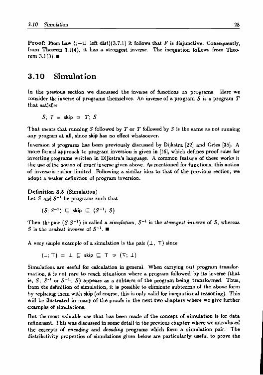
310 Simulation

In the previous section we discussed the inverse of functions on programs Here we consider the inverse of programs themselves An inverse of a program S is a program T that satisfies

s T = skip = T 8

That means that running 8 followed by T or T followed by 8 is tbe same as not running any program at all since skip hM no effect whatsoever

Inversion of progralTlS hM been previously discussed by Dijkstra [22] and Gries [35] A more formal approalth to program inversion is given in [16] which defines proof rules for inverting programs written in Dijkstras language A common feature of these works is the use of the Dation of etaet inverse given above As mentioned for functions this notion of inverse is rather limited Following a similar idea to that of the previous section we adopt a weaker definition of program inversion

Definition 35 (Simulation) Let 8 and 8-1 be programs such that

(s S-) lt skp lt (S- S)

Then the pair (88-1 ) 1S called a simulation 8-1 is the strongest inverse of 8 whereas 8 is the wealcest inverse of 8-1bullbull

A very simple example of a simulation is the pair (1 T) since

(1- T) = 1 lt skp lt T = (T 1)

Simulations are useful for calculation in general When carrying out program transforshymation it is not rare to reach situations where a program followed by its invertte (that is 8 S-1 or 8-1 8) appears as a subterm of the program being transformed Thus from the definition of simulation it is possible to eliminate subterms of the above form by replacing them with skip (of course this is only valid for inequational reamp60ning) This will be itlustrated in many of the proofs in the next two chapters where we give further examples of simulations

But the ID08t valuable use that has been made of the concept of simulation is for data refinement This was discussed in some detail in the previoW chapter where we introduced the concepts of encoding and decoding programs which form a simulation pair Tbe distributivity properties of simulations given below are particularly useful to prove the

correctness of the change of data representation phase of the compilation prltlClSS where the abstract space of the BOurce program is replaced by the concrete state of the target machine The appropriate encoding and decoding programs will be defined when the need arises

A detailed discussion on simulations can be found in [5] (where it is called illverse commiddot mands) and in [45] Here we prcBent some of the properties of simulation As should be expected these are similar to the oneEI given in tbe previous Bection

Theorem 32 (Simulation) Let S be a program The following properties hold (1) S-1 is unique if it exists (2) S-l exists if and only if S is universally disjunctive (3) S-I is universally conjunctive if it existsbull

We define the following abbreviations

Definition 36 (Simulation functions) Let (SS-1) be a simulation We use Sand S-l themselves as functions defined by

S(X) S X S- S-(X) S- X S

bull The next theorem shows that the concepts of simulation and approximate inverse are closely related

Theorem 33 (Lift of simulation) Let S and S-1 be simulation functions as defined above Then S-1 is the strongl5t inverse of S Furthermore rom Theorem 31 (StrongeElt inverses) we have

S(S-l(X)) i X i S-l(S(X))

bull The following tbeorem shows how simulation functions distribute through all the language operators introduced so far with a possihle improvement in the distributed result

Theorem 34 (Distrihutivity of simulation functions) (1) S(1) = 1 (2) S(T) i T (3) S(skip) i skip (4) S(X Y) i S(X) S( Y) (5) S(nP) i n X X E 1 S(X) (6) S(UP) = UX X E 1 S(X)) (7) S(p X bull F(X)) i p X bull S(F(S-l(X)))

311 AsSumptjOD amplid AsserUOD ro

311 Assumption and Assertion

The assumption of a condition b designated as bT can be regarded ae a miraculous test it leaves the state unchanged (behaving like slOp) if b is true otherwise it bebaves like T The assertion of b h also behaves like skip when b is true otherwise it fails behaving like l

The intended pUIpose of asswnptio~ and assertions is to give pret(Jnditions and postconshyditions respectively the status of programs For example

aT pj bL

is used to express the fact that the assumption of a is an obligation placed on the environshyment of the program p If the environment fajJs to provide a state Batisfying a aT behaves like a miracle tws saves the programmer from dealing with states not satisfying a since no program can implement T On the other hand an assertion is an obligation placed on the program itself If p fails to make b true on its completion it ends up behaving like abort

The first three laws formally state that the as5umption and tbe Msertion of a true condishytion are equivalent to skip that the assumption of a false condition leads to miracle and that the assertion of a false condition leads to abortion

Law 3111 trueT = trueL = skip (bT bL true cond)

Law 3112 false T = T (b T fl rood)

Law 3113 fa1seL L (bL fal rood)

Two consecutive 8a8umptions can be combined giving rise to an assumption of tbe conshyjunction of the original conditions tbis obviously means tbAt if any of tbe conditions is not satisfied the result will be miraculous An analogous law holds for assertions

Law3llA (aT bTl (all b)T (aTUbT) (b T conjunction)

Law 3115 (aL bL) (a II b)c (aL n b) (bL conjunction)

The iUlsumption of the disjunction of two conditioDB will behave like a miracle if and only if none of the conditions are SAtisfied There is a similar law for Msertions

Law 3116 (a V b)T (aTnbT) (bT disjunction)

Law 3117 (a V b)c (aL U bL) (bL disjunction)

It doe not matter if Achoice is made before or after an assumption (or an assertion) is executed

Law 3118 bT (p n q) (bT p) n (bT q) W-n dist)

Law 3119 b (p n q) = (b p) n (b q) (h -n disl)

The next law states that (bolt bT ) is a simulation

Law 31110 (b bT) = b ~ skip ~ bT = (b T b) (bL - bT simulation)

An assumption commutes with an arbitrary program p in the following sense (A similar law holds for assertions but we do not need it here)

Law 31111 If the free variables or b are not assigned by p

(p bT) ~ (b T p) (b T Pcommute)

The inequality occurs when b is false and p is 1 in which case the left-hand side reduces to 1 whereas the right-hand side reduces to T

312 Guarded Command

The standard notation b --10 P stands Cor a guarded command If the guard b is true the whole comrnand hehaves like p otherwise it behaves like T This suggests that a guard has the same effect as an assumption of the given condition which allows us to define a guarded command as follows

Definition 37 (Guarded command)

b-tp ~~ bT P

bull The laws or guarded conunands can therefore be proved from the above definition and the laws of sequential composition and assumptions

Law 3121 (true--+ p) = p (~ true guard)

Law 3122 (flse ---gt p) = T (_ fal guard)

Guards can be unnested by taking their conjunction

Law 3123 a _ (b ---gt p) = (a f b) _ p (~ guard conjunction)

Guards distribute over n


Law 3124 b~(p n q) = (b~p) n (b~ q) (gd - n dit)

The demonic cboice of guarded commands can be written as a single guarded comrnand by taking the disjunction of their guards This is easily derived from the last two laws

Law3125(a~p n b~q) = (aVb)~(a~p n b~q)

(- guard disjunetionl) Proof

RHS

laquoguard - n dit)(3124)

(aVb)~(a~p) n (aVb)~(b~q)

(~ guard conjunction)(3123))

LHS

bull When p and q above are the same program we have

Law 3126 (a~p)n(b~p) = (aVb)~p (_ guard disjunetion2)

Sequential comp~ition distributes leftward through guarded conunands

Law 3127 (b ~ pi q = b ~ (p q) ( - ~ left dit)

313 Guarded Command Set

Our main use of guarded commands is to model the possible actions of a dettJministic exshyecuting mechanism The fact that the mechanism can perform one of 11 actions according to its current state can be modelled hy a program fragment of the form

b1-10 actionl n n b -t action

provided bt b are pairwise disjoint Inatead of mentioning this disjointness condition explicitly we will write the above as

b1_ actionl D 0 b -t action

Strictly 0 is not a new operator of our language It is just syntactic sugar to improve conciseness and readability Any theorem that uses 0 can be readily restated in tenns of n with the associated disjointness conditions As an example we have the following law

]pound one of the guards of a guarded coIIUlULDd set holds initially the associated command will always be selected for execution

Law 3131 a --t (a --t pO b --t q) = a --t p (0 elim) Proof The proof relies on the (implicit) Msumption that a and b are disjoint (or a 1 b = false)

a-+(a --+p n b--tq)

(gud - n dit)(3124)

a -+ (a --+ p) n a --t (b -+ q)

(~ guard conjunction)(3123)

a --t p n false -+ q

(~ false guard)(3122) and (n- T unit)(342)

a~p

bull Other laws and theorems involving 0 will be described as the need arises

314 Conditional

A conditional coffillland has the generalllyntax p ltl b tgt q which is a concise fonn of the more usual notation

if b then p else q

It can also be defined in terms of more basic operators

Definition 38 (Conditional)

(plt1blgtq) 2 (b~pO~b~q)

bull The most basic property of a conditional is that its left branch is executed if the condition holds initially otherwise its right brancb is executed

Law 3141 (a b)T (p lt1 b V c Igt q) = (a b)T p (lt1 Igt true cond)

Law 3142 (a ~b)T (p lt1 b c Igt q) = (a ~b)T q (lt1 Igt false cond)

The left branch of a conditional can always be preceded by an assumption of the condition Similarly to precede the right branch by an assumption of the negation of the condition has no effect

Law 3143 (b T p ltl b Igt q) (plt1blgtq) (p lt1 b Igt ~bT q) (lt1 Igt void bT)

315 A3signment 34

If the two branches are the same program the conditional can be eliminated

Law 3144 p ltI b tgt P = P (ltI Igt idmp)

Guard distributes through the conditional

Law 3145 a _ (p ltI b Igt q) = (a _ p) ltI b Igt (a _ q) (guard - ltI Igt dit)

Sequential composition distributes leftward through the conditional

Law 3146 (p ltI b Igt q) = (p ltI b Igt q j ( - ltI Igt Ift dit)

The following two laws allow the elimination of nested conditionals in certain cases

Law 3147 P ltI b Igt (p ltI c Igt q) pltlbVctgtq (ltI po cond disjunction

Law 3148 (p ltI b Igt q) ltI c Igt q = P ltI b 1 c Igt q (ltI tgt cond conjunction

We have considered assumptions and assertions aB primitive commands and have defined guarded commands and the conditional in terms of them The following equations show that an alternative could be to consider the conditional as a constructor and regard assumptions assertions and guarded commands as special cases These are not stated all

laws because they are unnecessary in our proofs

bi skip ltI b tgtl bT skip lt1 b po T b_p =pltlbtgtT

315 Assignment

The command z = e stands for a multiple assignment where x is a list of distinct variables and e Ul an equalmiddotlength list of expressions The components of e are evaluated and simultaneously assigned to the corresponding (same position) components of x For example

XII= yz

swaps the values of z and II For simplicity we alIsume that the evaluation of an expression always delivers a result so the alIsignment will always terminate Furtbermore the validity of most of the laws relies on the falaquot that expression evaluation does not change the value of any variable that is no sidemiddoteJect is allowed

Obviously the assignment of the value of a variable to itself does not change anything

Law3151 (= 0) = skip (= lcip)

In fad such a vacuous assignment can be added to any other assignment without cbanging its effect

Law 3152 (z y= y) = (z= ) (= identity)

The list of variables and expressions may be subjected to the same permutation without changing the effect of the assignment

Law 3153 (zyz =e9) = (yzz=feg) 1= ym)

The sequential composition of two assignments to the same variables is easily combined to a single assignment

Law 3154 (z= e z = f) = (z= flz ~ j) (= combination)

Recall that f[z _ e] denotes the substitution of e for every free occurrence of in f

If the value of a variable is known the occurrences of this variable in an expression can be replaced with that value

Law 3155 (z = ) ~ (y =f) = (z = j ~ (y= flz ~ j) (= substitution)

Assignment is universally conjunctive

Law 3156 z= e nP = nIx X E P (z = X)) (= - n right dt)

Assignment distributes rightward through a conditional replacing occurrences of the asshysigned variables in the condition by the corresponding expressions

Law 3157 z= (p ltl b Igt q) = (z= i p) ltl biz ~ ]1gt (z = q) (= - ltl Igt right dil)

Similarly assignment commutes with an assertion in the following sense

Law 3158 (z= i bL ) = (b[z ~ )h z = (= -h commutation)

316 Generalised Assignment

The notation E b stands for a generalised assignment command Whenever p08Sible Z

is assigned an arbitrary value that makes the condjtion b hold but if no such value exists the assignment hehaves like T

Law 3161 (zE false) = T (E faLoe cond)

316 Generalised Assignmetlt 36

On the other hand a true condition imposes no constraintamp on the final value of In this case the generalised assignment is less deterministic than skip because it might leave everything unchanged

Law 3162 (xE true) r skip (E true cond)

To follow a generalised assignment by an assumption of the sAme condition has no effect if the assignment establishes the condition the assumption behaves like skip otherwise the assignment itself (and consequently its composition with the assumption) behaves like T

Law 3163 zE h hT = zE h (E void bT)

A similar law holds for assertions

Law 3164 zE h hJ xE h (E void bLl

A generalised assignment is refined by an assumption of the same condition The reason is that the final values of the variables of the assignment are arbitrary whereas the assumption does not change the value of any variable Actually an assumption can be regarded as a generalised assignment to an empty list of variables

Law 3165 (I E b) ~ bT ( E refined by bT)

Generalised assignment distributes rightward through the conditional provided the folshylowing condition is observed

Law 3166 If z does not occur in h I E a (p ltl b Igt q) = IE a p ltl b Igt I E a q) (E - ltl Igt rigbt dist)

Tn general an assignment cannot be expressed in terms of a generalised Msignment only For example there is no generalised assignment that corresponds to the assignment

x + 1 The reason is that we have not introduced notation to allow the condition of a generalised assignment of the form E h to refer back to the initial value of z But r e can always be written as a generalised Mampignment whenever the expression e doeB not mention z

Law 3167 IT e does not mention

zE(=e) = =e (E -= conversion)

If z and 11 are to be assigned arbitrary values (in sequence) to make a given condition hold we CAD reduce the nondeterminism by ensuring that the same (arbitrary) value is assigned to both r and y

Law 3168 If h does not mention 11

(z E b VE ~( - vI) ~ (ZE b v= I) (E efined by =)

We can commute the order of execution of an assignment and an arbitrary program p provided no interference occurs with the global variables

Law 3169 H no free variables of b nor are assigned by p (p x E b) ( (E b p) (x E b p commute)

The inequality occurs when p is 1 and the assignment results in T

317 Iteration

We use bp to denote the iteration commaod It is a concise form of the more conventional syntax

while b do p

Iteration can be defined as a special case of recursion

Definition 39 (Iteration)

b p t pX laquop X) 4 b tgt kip)

bull As iteration is a derived operator in our language we are able to prove (rather than just postulate) some of its properties This illustrates the modularity provided by the algebraic laws in developing more elaborate transformation strategies from the basic ones These strategies are largely used in the next two chapters substantially simplifying the proofs of normal form reduction

If the condition b does not bold initially the iteration b bull p behaveslike skip otherwise it behaves like p followed by the whole iteration

LawS171 (aA~b)T bp = (aA~b)T ( elim) Proof

LHS

Definition 39(lttioo) and (p fixed poiot)(381)

(a A ~b)T ((p b p) 4 b tgt skip)

(4 tgt false rood)(3142) and (-skip uoit)(331)

RHS

bull

317 Iteration 38

Law 3172 aT j (a Y b) p aT p (aYb)p ( unfold) Proof

LHS

~ Definitioo 39(lteration) and (p fixed point)(381)) aT (p (aVb)pltl (aVb) ~slcip)

~ (ltI ~ true cond)(3141)

RHS

bull A recurrent step in our proofs is to unfold ampD iteration and simplify the unfolded body when this is a guarded command set

Law 3173 Let R = (a -+ p 0 b -+ q) Then aT (aV)R ~ aT p (aVb)R ( - 0 unfold) Proof From ( unfold)(3l72) and (0 elim)(313l)bull

A guarded command set within an iteration can be eliminated if the condition of the iteration allows only one of the guards to hold

Law 3114 Let R= (a -+ p 0 b -+ q) Then a R ap ( - 0 elim) Proof

LHS

~ Definition 39(lteration) and (ltI void bT)(3143) pX bull (a T R X) ltI a slcip)

(o elim)(3131) pX laquoaT p X) ltI a ~skip)

( ltI ~ void bT)(3143) and Definition 39(Ileration)

RHS

bull The following allows the replacement of a guarded command inside an iteration

Law3175 LetR~(a _p 0 b_q) If r (aVb)R p (aVb)R then (aVb)(a_rob_q) (aVb)R ( replace guarded command) Proof

RHS

Definition 39(Ileration) and (p fixed point)(381))

(R RHS) ltl a Vb tgt skip (-n left dist)(371) (a --gt (p RHS) 0 b --gt (q RHS)) ltl a V b tgt skip

~ Assumption

(a --gt (r RHS) 0 b --gt (q RHS)) ltl a V b tgt skip ( -n left dist)(371)

((a --gt rOb --gt q) RHS) ltl a vb tgt skip

The final result follows from (p least fixed point(382)bull

The following law establishes the connection between tail-recursion and itealion ILs proof illustrates the use of approximate inverses of programming constructs

Law 3176 (hp) q = pXo((p X)ltl b tgtq) (-p tlrecuion) Proof (LHS J RHS)

Definition 39(Iteration) and (p fixed point)(381)

LHS = ((p h p) ltl b tgt skip) q ~ (- ltl tgt left djt)(3146) and (-skip unit)(331)

LHS = (p LHS) ltl b tgt q =gt (p least fixed point)(382)

LHS J RHS

(RHS J LHS)

(p fixed point)(381)

RHS = (p RHS) ltl b tgt q

=gt From Lemma 31(Strongest inverse of ) we have (RHS q) q ~ RHS

RHS J (p (RHS q) q) ltl b tgt q

~ (- ltl tgt left dit)(3146) and (-skip unit)(331)

RHS J ((p (RHS q)) ltl b tgt skip) q =- Definition 34(Approximate inver8ell)

(RHS q) J (p (RHS q)) ltl b togt skip =gt (p least fixed point)(381) and Definition 39(Iteration)

(RHS q)J bp

= Definition 34(Approximate inverses)

RHS J LHS

bull The following law is surprisingly important mainly in proving the corrednCSA of the normal form reduction of sequentiaJ composition Ita proof without assuming continuity of the language operators is originally due to Gardiner and Pandya 125

318 Statjc Declaration 40

Law 3177 (b p) (b V e) P = (b V e) P ( sequenre) Proof (RHS ) LHS)

(4 lgt idemp)(3144)

RHS = RHS 4 b lgt RHS _ (Definition 39(Iteration) and (p fixed point(381)

RHS = ((p RHS) 4 b Velgt skip) 4 b lgt ((b V e) p)

~ (4 lgt void bT (3143) and ( elim)(3171)

RHS = ((Pi RHS) 4 bVe lgt(bVe)p)ltl b lgt((bVe)p)

= (4 lgt cond conjunction)(3148)

RHS = (Pi RHS)ltl b lgt((bVe)p) =gt (p least fixed point(382)

RHS) pXo(p X)ltl b lgt((bVe)p) _ ( - p tail recurnion)(3176)

RHS ) (bp) ((bVe)p) ~ RHS ) LHS

(LHS ) RHS)

(Definition 39(lteration) and (p fixed point(381)

LHS = ((qi (bp))4 b lgtskip) (bVe)p

= (i- 4 lgt left dit(3J46) and (-skip unit(331)

LHS = (p LHS) 4 b lgt RHS ~ (p fixed point)(381)

LHS = (Pi LHS) 4 b lgt ((p RHS) 4 bVelgt skip)

(4 lgt cond dijunction(3J47) and LHS [ RHS) LHS ) (Pi LHS) 4 bVelgt skip

(Definition 39(lteration) and (p least fixed point(382))

LHS ) RBS

bull

318 Static Declaration

The notation dec x bull p declares the list of distinct variables ~ for use in the program p (tbe scope of tbe declaration) Local blocks of this form may appear anywhere a program is expected

It does not matter wbether variables are declared in one list or singly

Law 3181 If x and V bave no variables in common decx(decyep = dec~yep (dec assoc)

41 318 Static Declaration

Nor doee it matter in which order they are declared

Law 3182 decz(decyep) = decye(deczp) (dec aym)

If a declared variable is never used its declaration has no effect

Law 3183 If z is not free in p deczep = p (dec elim)

One can change the name of a bound variable provided the new name is not used for a free variable This law is normally stated as follows

decr e p = dec y e p[z +- yJ provided y is not free in p

where the clashes of y with bound variables of p are dealt with by the renaming implicit in the substitution operator However this law justifies transformations which are not always valid (in the context of our language) For example consider tbe recursive program

(1) dec 0 (I XoF(decoX))

Because of static scope rules any free occurrence of z in F is bound to the outer declashyration ofr The inner declaration of z has no effect since its scope does not include F and therefore it can be eliminated

(2) dec 0 (I X 0 F(X))

However renaming of bound variablee as stated above allows (1) to be transformed into (assuming that y is not free in F)

dec 0 (I X 0 F(decy 0 XI ~ yJ))

which is clearly distinct from (2) if there are free occurrences of x in F The incoDBistency arises from the fad that the application of the law identified the occurrence of t bound to the inner declaration with the (possible) occurrences bo~d to the outer declaration this violatee the concept of static scoping One way to avoid the problem is to add an extra condition to the law about renaming of locaJ variables This requires the following concept

Definition 310 (Contiguous scope) We say that a variable x has a contiguous scope in a program p if

e p contains no free program identifiers (standing for call commands) or

e if X is free in p then x is not free in (the program defining) X

bull

~


The concept also applies when X is the name of a procedure which will be dealt with in Chapter 5 The law then becomes

Law 31811 If V is not free in P and z has a contiguous scape in p then dec z _ p = dec yo p[z _ y (dec rename)

We can ensure that programs will always have contiguous scope (With respect to any local variable) by requiring that nested declarations always use distinct names for variables (which are also distinct from the names used for global variables) When applying the above law we will assume that the condition of contiguous scope is aI ways satisfied

The value of a declared variable is totally arbitrary Therefore initialisation of a variable may reduce nondeterminism

Law 3185 (1) declp deczz=e p (dec-= initial value) (2) deczp deczzE b p (dec-E initial value)

An assignment to a variable just before the end of its scope is irrelevant But a generalised assignment cannot be completely ignored since it roay result in a miracle

Law 3186 (1) dec p dec z bull p z = e (dec-= final value) (2) decp l dec z _ p z E b (delt- E final value)

The scope of a variable may be increased without effect provided that it does not interfere with the other variables with the same name Thus each of the programming constructs has a distrihution law with declaration For example if one of the arguments of the sequential composition operator declares the variable z then the 8cope of the declaration can be extended with the other component provided there is no capture of free variables

Law 3187 If z i8 not free in q

(1) (de 0 p) q = decz 0 p q (-dec left dit) (2) q (deczop) = deczoq p ( -dec right dit)

When both arguments declare the 8ame variable the two declarations can be replaced with a ingle one

Law 3188 (decz _ p) (decz _ q) ~ decz _ Pi q (dec- dit)

But note that this may reduce nondeterminism Consider the case where q is y =

Then the final value of y on the left-hand side of the above inequation would be totally arbitrary On the right-hand side however it may be the cue that z was asaigned a value in p thus the final value of y would be that of z In aU cases the right-hand side is at least 8B deterministic as the left-hand side

~

319 Dynamic Dec1aratjon 43

If each Mgument program of a guarded command set or conditional declares the variable x then the declaration may be moved outside the comltructor provided that does not occur in the guards or in the condition

Law 3189 IT z does not occur in a or b a _ (dec x e p) 0 b _ (decx e q) = dec x e a _ pO b _ q (delt - 0 diat)

Law 31810 IT x does not occur in b (decxep)lttblgt(decxeq) = decxeplttblgtq (dec - 0 lgt dist)

Note that it is possible to deal with cases where x is only declared in one of the branches (and is not free in the other one) by using Law 3183

Declaration can also be moved outside an iteration possibly reducing nondeterminism As shown below this law can be derived from more basic ones

Law 31811 IT x does not occur in b b(decxep) b deczebp (dec - dist) Proof

(Definition 39(Iteration) and (p fixed point)(381)

RHS = dec 0 (p b p) ltl b lgt skip (dec - ltt lgt dit)(31810) and (dec elim)(3183)

RHS = (dec 0 p bgt p) ltl b lgt skip =gt (dec- dist)(3188)

RHS~((decop) RHS)ltl b lgtskip =gt Definition 39(Iteration) and (p least fixed point)(382)

RHS ~ LHS

bull

319 DynaInic Declaration

The command war x introduces a dynamic scope of x which extends up to

e the end of the static scope of x or

e the execution of the command end x

whichever comes first

An operational argument may help to clarify how the two kinds of declaration differ The general idea is to associate an unbounded stack with each variable One can think of a static declaration of x as introducing a new variable (which is assigned an arbitrary value)


witb its (implicit) unbounded stack which is initially empty Rather than creating a new variable the commands for dynamic declaration operate OD this stack The effect of var is to push the CWTent value of onto the stack assigning to an arbitrary value end pops the stack and assigns the popped value to If the stack was empty this value is arbitrary

Recall from Section 26 that having separate conunands to introduce and end the scope of a variable is an essential feature to define the encoding and decoding progtampm8 used in our approacb to data refinement the encoding program introduces the abstract state and ends tbe scope of the concrete state whereas the decoding program introduces the concrete state and ends the scope of the abstract state

var and end obey laws similar to those of dec Both val and end are associative in the sense described below

Law 3191 If x and y have no variables in common (1) (val x vary) = varzy (var assoc) (2) (end endy) = endzy (end assoc)

The (dynamic) scope of a variable may be increased without effect provided that this does not interfere with other free variables

Law 3192 If x is not free in p

(1) Pi varz = varj P (var change scope) (2) endi P = Pj end (end change scope)

Both var and end dUitribute rightward through the conditional as long as no interlerence occurs with the condition

Law 3193 H b does not mention x

(1) (vorr p)lt1 b tgt(varr q) varr (plt1 b tgtq) (var - ~ tgt right dist) (2) (endr p)lt1 b tgt(endr q) endr (plt1 b tgtq) (end - lt1 tgt right dit)

As explained above val x assigns an arbitrary value to z The nondetenninism can be reduced by initialisation of z

Law 3194 (1) varx b (valxi = e) (var-= initial value) (2) varz b (varx E b) (var-E initial value)

An assignment to a variable just before the end of its scope is irrelevant But a generalised assignment cannot be completely ignored as it may result in a miracle

Law 3195 (1) d r (r e end r) (nd- final value) (2) d r I (rE h end r) (end-E final value)


The next two laws ampre essential for reasoning about data refinement They are precisely the ones that assign the dynamic declaration semantics to var and end The first law says that end Z followed by var z leaves all variables but z unchanged var z followed by end z has no effect (even on z) Therefore the pair (end z var z) is a simulation

Law3196 (endxvarz) l skip = (varzendz) (end - var simulation)

The second law postulates that the sequential composition of end z with var z has no effect whenever it is followed by an assignment to z that does not rely on the previous value of x Law 3197 (endzj varz zE b) = zE b (end - var skip)

Observe that the syntax of static deciaration (dec) promptly disallows the above two laws since there is no separate construct to end the scope of a valiable

The following laws relate the two kinds of deciacation They formalise the intuitive meanshying given in the beginning of this section

If the first command in the scope of a static declaration of z is var z or end z this command has no effect

Law 3198 (1) decz varz p = decz p (var eliml) (2) decz endzj p = decz p (end eliml)

First we give an operational justification of (1) Recall that a static declaration of z create an implicit stack which is originally empty Then the effect of var z on the leftshyhand side of (1) is to push the current value of z (which is arbitrary) onto this stack and to assjgn an arbitrary value to z But the value of z was already arbitrary thus the assignment has no effect Furthermore the effect of pWlhing an arbitrary value onto the empty stack is also immaterial The only command that may access this value is a subsequent end z which would assign an arbitracy value to z if the stack Wall empty anyway The justification of (2) is simpler As the stack associated with z is initially empty the effect of end z is to assign an acbitrary value to z hut the value of z was already arbitrary

As we said before the dynamic scope of a variable z cannot extend further than its static scope Therefore starting or ending a dynamic scope of z just heCore the end of its static scope is irrelevant

Law 3199 (1) deczPi varz decz p (var elim2) (2) dec x bull p end x = decz p (endlirn2)

In some ase8 there is no need to distinguish between a static and a dynamic scope of a given variable To state this law we need two auxiliary concepts One is that of a contiguous scope as defined in the previous aection (Definition 310) The other is defined below

319 Dynmc Declaration 46

Definition 311 (Block-structure) A program p is block-structured with respect to a variable z if each dynamic declaration of z in p (vatr) has a corresponding staticaJly determined undeclaration (end r) More precisely

1 all programs that do not contain the commands var x or end z axe block-structured with respect to ri

2 if P is block-structured with retlpect to z 80 is var Pi endr

bull Then we have the following law

Law 31910 IT P is block structured with respect to x and x has a contiguous scope in p then decr bull P = var Xi Pi endr (dec - (var end) conversion)

From the above we derive the following law about introduction of local declarations

Law 31911 IT P is block structured with respect to x and x hAS a contiguous scope in p then r E bj P rE c = (decrE b P)i x E c (dec introduction)

Proof

LHS

(end - V kip)(3J97))

end Xj var r r E bi Pi end x va rj E c

(dec - (v end) coQverioQ)(31910))

end Zj (dec x bull xE bi p) var i E c

= (end change cope)(3192))

(decx bull x E b p) end j var x Z E c

(end - valt kip)(3197))

RHS

bull The above two laws will be used in the next chapters to perform transfonnations on source programplll8 These are always block-structured since var and end are not part of our 80urce language In the previous section we explained how to ensure that programs always have contiguous scope (with respect to any locaJ variable) Therefore these laws will be applied assuming that these conditions are always satisfied

320 The Correctness of the Basic Laws

In a purely algebraic view the laws of a given language are an algebraic semantics for this language There is no place (or the task of verifying the validity of the more basic Laws they are axioms w hieb express the relationship between the operators of th~ language However the method of postulating is questioned by those who aUow a model-oriented approach eopecially when the set of axioms is relatively large as it is here Poatulating an inconsistent set of laws could be a disaster it would allow one to prove invalid results like the correctness of an inaccurate compiler

The way to avoid this danger is to link the algebraic semantics of the language with a mathematical model in which the laws can be proved For example Hoare and He [46J provide a relational model (or programs where the correctness of the laws could be esshytablished by appealing to the calculus of relations [71] Another model that hiLS gained widespread acceptance is the predicate transformer model of Dijskstra [21] which was briefly discussed in the previous chapter In this case the semantics of each language construct (that is its weakest precondition) is given and the laws are verified by appealshying to the predicate calculus

It is also possible to link the algebraic semantics of the language to a more concrete (operational) model This allows to check for feasibility (implementability) of the language operators But in our case this is not possible as our language includes non-implementable operators

Once the laws have been proved in whatever model they should serve as tools for carrying out program transformation The mathematical definitions that allow their verification are normally more complex and therefore not appealing to practical use This separation of concerns is well described in [42] which explores the role of algebra and models to the construction of theories relevant to computing

But even aIter the model has served its intended purpose additional remIts of practical interest can be achieved For example from the experience in the application of basic algebraic laws of programming to 90lve a given task one discovers more elaborate transshyformation strategies that allow more concise and elegant proofs This was illwtrated in the section on iteration where all the laws were derived from more basic oneo

In the remainder of this section we use the predicate transformer model to illustrate how tbe basic laws of our language can be verified

Predicate Transformers

We deal only with a few language operators Their definitions as predicate traneformers were given in the previous chapter but are repeated here for convenience In the fQUowing a ranges over the set of predicates p and q stand for arhitrary programs and P for an

320 The Correctness of the Basjc Laws 48

arbitrary set of programs

skip ~ )00

L ~ ) a bull false

T ~ )aetrue

UP ~ao(3X EPoX(a))

np ~ao(VXEPoX(a)) p q ~aop(q(a))

The definition of the remaining operators can be found for example in [5J From the above definitions we can prove the laws of the corresponding operators For example from the definition of ~ we CaD derive its characterisatloD in terms of weakest preconditions

p~q

_ Definition 31(The ordering Relation)

(p n q) = p

-= Definition of n (~a 0 p(a) q(a)) = p

= The axiom of extensionality

Va 0 (p(a) q(a) pta)) = Predicate calculus

Va 0 (p(a) =gt q(a))

which corresponds precisely to the definition of refinement adopted in all approaches to the refinement calculus based on weakell preconditions as discusaed in the previous chapter As another example we verify Law (u-n dist)(372)

(up)np

Definition of n

~ a 0 (UP)(a) p(a) Definition of U

~ a 0 (3X EP 0 X(araquo p(a) Assuming that X is not free in p ~ a 0 (3 X E P 0 (X( a) 1 p( a))) Definition of n)

~ao(3XEPo(Xnp)(araquo)

Set theory ~ a 0 (3 X E X X E P (X n p)) 0 X(araquo

= Definition of U UX X EP (X np))

Chapter 4

A Simple Compiler

Setting up equations is like translating from one lanshyguage into another

- G Polya

In the first two sections of this chapter we describe the nonnal form as a model of an arbitrary executing mechanism The normal form theorenJB of Section 42 are concerned with control elimination the reduction of the nested control structure of the source program to a single flat iteration These theorems are largely independent of a particular target machine

In the subsequent sections we design and prove the correctness of a compiler for a subset of our source language not including procedures or recursion (which are dealt with in the next chapter) The constructions considered here are skip assignment sequential composition demonic nondeterminism conditional iteration and local declarations

As described earlier we split the compilation process into three main phases simplifishycation of expressions control elimination and data refinement (the conversion from the abstract space of the source program to the concrete state of the target machine) The control elimination phase in particular is directly achieved by instantiating the generic theoreIllil of Section 42

Every theorem directly relevant to the compilation process has the status of a MLle Each rule expresses a transformation which brings the source program closer to a normal form with the same structure as the target machine The final section shows that taken collectively these rules can be used to carry out the compilation task

It is important to emphasise the different roles played by the algebraic laws described in the previous chapter and these reduction rules the laws express general properties of the language operators whereaB the rules serve the special purpose of transforming an arbitrary program to a normal fonn The laws are necessary to prove the rules and these (not the laws) are used to carry out compilation

49

41 The Normal Form 50

41 The Normal Form

A program of the form

dectletlEa bp CL

can be interpreted a8 a very genera model of a machine executing a stored program computer in the following way

bull The list of variables 17 represents the machine components (for example registers) They are introduced a6 local variables since they have no counterpart at the BOurCe level thexefore their final values are irrelevant

bull a is an aasumption about the initial state if it is impossible to make a true by aasigning to v the machine behaves miraculously

e p is the stored program it is executed until the condition b becomes false Usually p will be a guarded command set of the form

bt-Plo ob-p

Wbenever the machine is in state bi the action (or instruction) p is executed In this case the condition b Is given by

V V D

bull c is an assertion about the final state of the machine if execution of the stored program does not assert c the machine ends up behaving like abort

Notice that upon termination of the iteration b p b is false and we have

bp CL = bp (bhi CL = bp (btch

Thus ~bere is no loss of generality in assuming that c = (b t c) and consequently that (b t c) = false The normal form thoorems will rely on the assumption that b and care disjoint

A normal form program will be abbreviated a6 follows

Definition 41 (Normal form)

1 [a b _ p c) ~g dcco tIE a b p CL where (b t c) = false

bull For convenience we will sometimes use the form

17 [a (b l _ 11deg 0 b - P) eJ as aD abhreviation of

[a (D V V D) ~ ( ~ PI 0 0 D ~ P) c)

42 Normal Fonn Reduction 5l

42 Normal Form Reduction

To reduce an arhitrary program to normal fonn it is sufficient to show how each primitive command can be written in normal form and how each operator of the language (when applied to operands in normal form) yields a result expressible in normal fonn The following reductions involve no change of data representation Therefore we can directly compare the source constructs with the associated normal fonn progranl8

If the initial state coincides with the final state the machine does not perform any action In more concrete terIrul the empty code is a possible implementation of skip

Theorem 41 (Skip)

skip ~ v [a b - p a]

Proof

RHS

( elim)(3171) remember a A b = false)

decv vE 6 61

HE void a)(3164) and (-skip unit)(331) dec v bull v E a skip

r (dec-E initial value)(3185) and (dec e1im)(3183)

LHS

bull The following lemma shows how a primitive command can be written in normal form Actually the lemma is valid for all programs p but we will not make use of it for nonshyprimitive constructs because we follow an innermost (bottom-up) reduction strategy

Lemma 41 (Primitive commands) If v is not free in p then

p ~ v [a 6 _ (p vE C) c]

Proof

RHS

( unfold)(3172) and ( elim)(3171)) dec v bull v E 6 p v E c C1

r (dec-E initial value)(3185) and (E void c)(3164)

dec v bull Pi v E C

r (dec-E final value)(3186) and (dec e1im)(3183))

LHS

bull


The following normal form representations of skip and assignment are instantiatioIlH of the above lemma The one of skip is further simplified by the fact that it ill an identity of sequential composition The operational interpretation is that skip can be implemented byajwnp

Theorem 42 (Skip)

skip ~ u[a(a_vEc)c]

bull Theorem 43 (Assignment)

z = e ~ v [a a -+ (z = e vE c) cJ

bull The reduction of sequential composition assumes that both arguments are already in normal form and that the final state of the left argument coincides with the initial state of the right argument The components of the resulting normal form are the initial state of the left argument the final state of the right argument and a guarded cornmand set that combines the original guarded commands

First we prove the reduction of sequential composition for the particular case where tbe guarded command set of the right argument includes that of the left argument

Lemma 42 (Sequential composition)

v[ab~pe] v [e(o )1 c v[a(o ~)cJ

Proof Let R = (b ~ p 0 b ~ q)

LHS

c (dec- dit)(3188)

dec tI e v E a h-t P Co v E co (bt V bz) Rj c

c (vE e refined by e )(3196) and (e - e simulation)(31110)

decvevEa b1 p (b1Vbz)R CJ

( - 0 elim)(3174)

dectTetTEaj btR (blVbl)R CJ

( sequenre)(3177))

RHS

bull

42 Normal Fonn Reduction 53

Now we show that the guarded command set of a normal form program can be reduced by eliminating arbitrary guarded commands We obtain amp program which is worse than the original one

Lemma 43 (Eliminate guarded command)

Igt ~ [a ( 0 b~

p)q

c] ) [a Igt ~ p c]

Proof LetR=(Igt~pO bo~q)

LHS

J Lemma 42(Sequential composition)

11 [a b1 --t p c) t1 [e R e] ) Theorem41(Skip) and (-skip unit)(331)

RHS

bull The reduction of sequential composition is proved directly from the above two lemmas These lemmaa will be of more general utility

Theorem 44 (Sequential composition)

[a b ~ p ] bull [ b ~ q c] lt [a (0 ~) c]

Proof

RHS

) (Lemma 42(Sequential composition)

[ab~p] [Co(O ~)CI ) Lemma 43(E1iminate guarded commaud))

LHS

bull The following lemma shows how to eliminate a conditional command when its branches are normampl form programs with identical components except for the initial state The first action to be executed in the resulting normal form program determines whith of the original initial states should be activated


Lemma 44 (Conditional) If v ie not free in b then

v [a R I ltl b Igt v la R j ~ v [a R j

a --+ (v E aJ 4 b tgt vE a-I))where R= (0 bl --+ P Proof

RHS ( - 0 unfold)(3173)

decv_Ea (vEa I 46 tgtvE~) (aVb1 )Rj c) (- ltl Igt left dit)(3146)

decv 0 v E a ((v E a (aV b) R ) ltl b Igt (v E a (a V 1gt) R )) (E - ltl Igt right dit)(3166) and (dec - ltl Igt dit)(31810) (deev _ v E a vE al (a V bt) R c)) 4 b tgt

(decv_vEa tlE~ (aVbt)R c)) J (dec- E initial vlue)(3185)

LHS

bull The above lemma is useful for intermediate calculations It 1S used in the proof of the normal form redudion of conditional and iteration commands

Theorem 45 (Conditional) If dOoeS not occur in b then

v [all bt --+ P cIl 4 b tgt v [~ ~ --+ q c] ~ v [a R c]

a --+ (vE al 4 b tgt 11E ~)) 61 --+ P 0 cl --+ v E cwheR= (~ b ~ q

Proof

RHS ) Lemm44(Conditional)

v [a R j ltl b Igt v la R j ) Lemmas 42(Sequential compition) and 43(Eliminate guarded command)

( [aJ ~ --+ P CI] v [CII CI --+ 11E C cJ) 4 b tgt v [~ l --+ q cJ

) Themem 42(Skip) and (-skip unit)(331) LHS

bull


The next leouna establishe9 a simple fact if the unique effect of the first guarded command to be executed is to make a certain expression trLle we may substitute the expression fOT the illitial state of the normal fonn program

Lemma 45 (Void initial state)

Co --- raquo E a) c eo ~ bull E a)[eo(o 6~p v [a ( 0 b -+ p cJ

Proof

LHS ( - 0 unfold)(3173))

( eo ~ bull E a)

dec v bull v E Co v E a (Co vb) 0 b -+ P cJ

~ (dec- E initial valuo)(3185))

RHS

bull In order to reduce an iteration oomrnand we asSUIJ)e that its body is in normal form Let ao and Co be the initial and final states of this nonnal fonn program The nonnal fonn of the whole iteration behaves ae follows The first action to be executed is a conditional command which tests if the oondition of the iteration holds in which case ao is activated otherwise the program reacbe9 its final state When Co is activated the guard of the first action is activated 80 that the conditional command is executed again

Theorem 48 (Iteration) If v does not occur in b then

6 bullbull [110 6 ~ p eoJ C [a R eJ

a~(EIIo6lgtEe)) where R = 0 Co -+ v E a

( o bl-+p Proof

RHS ~ Lenuna 44(CoDditional))

v [110 R cJ 6 lgt v [e R e) ~ Lemma 42(Sequential compoition) and Theorem 41(Skip))

v [ 1gt ~ p eo] v [eo R cJ b tgt kip ~ Lemma 45(Yoid initial tate))

(v [110 1gt ~ p eoJ RHS) 6 tgt kip

The final result follows from the above and (IJ least fixed poinl(382)bull

43 The Target MampcIllne 56

The nondetenninistic choice of two programs can be implemented by either of them We can actually eliminate the choice At the source level and avoid compiling one of the components

Theorem 47 (Nondeterminism)

(1) (pnq) I p (2) (p n q) I q

Proof From (I -n glb)(367)bull

43 The Target Machine

The compiler we design in the next three sections produces code foc a simple target machine which consists of four components

P a sequential register (program counter) A a general purpose register M a store for variables (RAM) m a stOre for instructions (ROM)

The idea is to regard the machine components as program variables and design the inshystructions as assignments that update the machine state

P and A will be represented by single variables Altbough we do Dot deal with types explicitly P will be assigned integer expressions standing for locations in ROM A will be treated as an ordinary source variable it will play 8Il important role in the decomposition of expressions which is the f1uhject of the next section M will be modelled as a map from addrcssel of locations in RAM to expresioD1l denoting the corresponding values and m as a map from addreses of locations in ROM to instructions

In order to model M and m we need to extend our language to allow map variables We use tbe foUowing operators on maps

z ~ e Singleton map ml U InJ union m ffi InJ overriding m[zJ application

Furtbennore we use the fonowing abhreviations

Zl bull Z~ el bull e 4 Zt~ etU Uz~ e m[ztmiddotmiddotz] ~ mfzd m[z)

In tbe first case we assume that no variable appears more than once in the list ZI bullbullbullbull zbull

One of the greatest advantages of algebra is abstraction An the laws of our language are unaffected by this exteD1lion In particular the laws of assignment and declaration CAn be

44 SffiJplificatjon of Expressions 57

readily used to manipulate map variables and expre5sions and no additional laws tlUn out to be necessary For example we can combine the two assignments

m=mlll[~ e m=mllly~1l

by using Law = combination3154 re5u1ting in

m=mlll~ e1lIy~1l

Similarly

m=mEflzl---+eendm

is equivalent to (from Law (end-= final value)(3195))

end m

The instructions of our simple machine are defined below We assume that n stands for an address in RAM and t for an address in ROM

lod( n) = AP=Mn]P+[store( n) = MP=(MIlI[n~A)P+

~ [bop-A(n) = AP~(AhopM n])P+

uop-A 2 AP=(uopA)P+

jump(k) ~ P=tcjump(k) = P~ (P + 1 ltl A 1gt k)

where

z= (et ltI b Igt e-l) = (z= el ltI b Igt = e1

and as before bop and uop stand for arbitrary binary and unary operators respectively

The normal form describing the behaviour of this machine is an iterated execution of instructions taken from the store m at location P

dPAP=8 (8~PltIlmIP] (P=h

where s is the intended start address of code and f the finish address The aim of the following sections is to show how an arbitrary source program can be reduced to this form

44 Simplification of Expressions

One of the tasks involved in the translation process is the elimination of nested expresaions The outcome of this phase is a program where each assignment is simple (lee definition below) Furthermore all the local variables are expanded to widest scope 0 that they can be implemented 88 global variables Of course this is valid only in the absence of recursion and it requires that all local variables have distinct names which must a1so be different from the names used for global variables


Definition 42 (Simple assignment) An aasignment is simple if it haa one of the forms

A=3 z =A A=Abopz A=uopA

where z is a source variablebull

These patterus are closely related to the ones used to define the instructions For example the first one will eventually turn into a load instruction the vilUiable P will appear as a result of the control elimination phase and z will be replaced by its memory location as a result of the change of data representation

Iu the remainder of this section we will show how to simplify expressions by using the register variable A and new local variables We assume that z is a single variable and e a single expression rather than arbitrary lists

The first rule transfonllB ampIl assignment into a block that introduces A as aloca1 variable

Rule 41 (Introduce A) If A doell not occur in z = e

(z=e) = decAeA=e z=A

Proof From the laws to combine assignment and eliminate local variablesbull

Note that the assignment z = A is already simple By transfonning all the assignments in this way we need only simplify expressions assigned to A The bext rule deals with unary operators

Rule 42 (Unary operator)

(A=uope) = (A=eA=uopA)

Proof From the law to comhine assignmentsbull

Observe that the second assignment on the right~hand side of the above equation is simple To deal with binary operators we need to introduce a fresh local variable t It plays the role of a temporary variable that holds the value of a subexpression

RUle 43 (Binary operator) If neither A nor t occur in e or J

(A=ebopf) = dectA= =A A=e A=Abop

44 Simp1iJication of Expressions 59

Proof

RHS (= combination)(3154) and (= identity)(3152))

decteA=j t= A=ebopt (= combillation)(3154) and (= identity)(3152))

dec 0 A = [ A= bop[ t = [ (= combination)(3154) (dec-= final value)(3186) and

(dec elim)(3183))

LHS

bull Again the only expressions that may still need to be simplified (e and f) are botb assigned to the variable A An exhaustive application of the above rules will simplify arbitrarily nested expressions turning every assignment into a simple one

When the expression above is a variilble it is unnecessary to create a temporary variilble to hold its value The following is an optimisation of the previous rule for this particular case

Rule 44 (Binary operator - optimisation) If A does not occur in e or x

(A= bopz) = (A= A= Abopz)

Proof From the law to combine assignmentsbull

Tbe boolean expressions appearing in iteration and conditional commands may also be arbitrarily nested and therefore need to be simplified

Rule 45 (Condition of iteration) If neither A nor v occur in b

b (decvA e p) decvA e A= bi A (Pi A= b)

Proof

RUS (p fixed point)(381)) decA 0 A= b ((p A= b A_ (p A= b)) ltl b tgt skip)

(= - ltl tgt rigbt dist)(3157l (dec - ltl tgt dist)(31810) aDd

(dec elim)(3183)) (decAoA=b p A=b A_(p A=b))ltl b tgtskip

J (dec- dist)(3188) and (dec-= initial value)(3185))

((decA 0 p) RUS) ltl b tgt skip

The result foUow8 from (p leoot fixed point)(382)bull


The local variable A on the left-band side of the above lDequation is a result of tbe simplishyfication of assignments in p LikewiBe t1 may be an arhitrary list of temporary variables created to simplify boolean operators or originally introduced by the programmer By moving these declarations out of the body of the iteration we avoid nested declarations of the variable A The expression b can now he simplified using the previous theorems

In a similar way we can simplify the boolean expressions of conditional statements

Rule 46 (Condition of conditional) If neither v nor A occur in b

(decAp) b cgt(deevAq) ( deltvAA~b (p A Cgtq)

Proof Similar to the one abovebull

The following theorem summarises the outcome of this phase of compilation

Theorem 48 (Expression simplification) For an arbitrary source program p there is a program q such that

pidecvA q

where q contains no local declarations all assignments in q are simple and the only boolean condition in q is the variable A Proof By structural induction using rules 41-46 together with the following laws

bull (-delt di(3187 3188) This is used to increase tbe scope of the local variables as much as possible

bull (de oe(3181) aDd (delt rename(3184) Tne former is used to eliminate nested declarations that may have been introduced by the programmer or resulted from the simplification of boolean operators the latter ie uJed to rename nested occurrences of variable which were declared with the same name so that the nesting can be eliminated

bull (delt elim)(3183) Rule 46 assumes that the local variables of the two hranches of a conditional are the same The above law CAn be used to introduce void declarations to ensure that this assumption will be satisfied

bull 45 Control Elimination

Recall that the machine considered here is equipped with a register P which is used for scheduling the eelection and eequencing of instructioD8 Thie can be simulated by regarding P as a variable in the foDowing way

45 Control Eliminatjon 61

bull Selection is achieved by representing the stored program as a set of guarded com~

manda each one of the form

(P=laquo)~q

meaning that q (standing for some machine instruction) will be executed when P has value k

bull Sequencing is modelled by incrementing P

P= P + 1

bull A jump to an instruction at memory location k is achieved by the assignment

P= laquo

Clearly the initial value of P must be the address of the location of the first instruction to be executed These conventions are our basis to transform the nested control structure of the source program into a single flat iteration which models the execution of a stored program The outcome of this section is a simple normal form program

Definition 43 (Simple normal form) We say that a normal fonn program is simple if it has the form

P[(P=)b~p(P=f)J

where p is a set of guarded cornrnands of the form

O9ltJ(P = k) -+ ejP= el dl

and b is the union of the guards (P = k) for all k such that s ~ k lt Furthennore the assignment ej P = e d follows one of the patterns used to define the machine instructions except that the source variables may not yet have been replaced by their corresponding memory locations (this is addressed in tbe next Mrlion)bull

Reduction to this simple normal form can be achieved by instantiating the normal form theorems of Section 42 taking into account the particular encoding of control state of our simple macbine In the following we abbreviate

P [(P = )b ~ p(P =f)J

to

P [b ~ pf]

The purpose of the first implementation of skip is to generate empty code false -lo skip is equivalent to T which is the identity of o


Rule 47 (Skip)

skip ( P [s false - skip s]

bull Rule 48 (Skip)

kip lt PI(P=s~P=+I)+lJ

bull Rule 49 (Assignment)

(x=e) lt P[(P=~(xP=eP+l))+l]

bull Rule 410 (Sequential composition)

(P Is b ~ Po]) (P Io Igt ~ qf)) lt P Is (0 ~ ~)f]

bull Rule 411 (Conditional)

(P Is + I b ~ Po]) 4 A lgt (P Ifo +I b ~ qf]) lt P [s R]

P = ~ P= (P + 14 A lgt 10 + I)) whereR= (~ bl -t pDP = 0 -t P =

ba -t q

bull Rule 412 (Iteration)

PI ( P=~P=(P+14Algtf+I))lo+lJA(PI+Ib~pk]) lt Ob_pOP=o-tP=s

bull It is worth observing that the above rules assume the allocation of contiguous addresses or the stored program For example the rule for sequential composition asstffiles that the finish address of the normal form program on the left coincides with the start address of the norma form program on the right


Strictly the above rules cannot be justified only from the reduction theorem8 of Section 42 Some additional (although trivial) transformations are required As an example we present the proof of Rule 49

P[a(P=a~(xP=eP+I))a+l]

(= ubtitution)(3155)

P [a (P = s ~ (x P = e a + I))a + IJ (= combination)(3154) and (= identity)(3152)

P [a (P = a ~ (x = e P = a + l))a + I] (E - = conversion)(3167)

P [s (P = a ~ (x = e P E (p = a + I))) a + 1] ] Theorem 43(Assignment)

x= e

The additional transfonnatiolls required to prove the other theorems are similar The next theorem summarises the outcome of this phase of compilation

Theorem 49 (Control elimination) Consider a program of the fonn

decvAmiddot9

where q contains DO local declaration all assignments in 9 are simple and the only boolean condition in q is the variable A Then there is a simple normal form program such that

decvA 0 q vAP [(P = a)b ~ r(P =J)]

Proof By structural induction using rules 47-412 we transform q into

P [(P = a) b ~ r (P = fJ]

The final result follows from (dec a8soc(3181)bull

46 Data Refinement

The only task that remains to be addressed is the replacement of the abstract space of the source program (formed from tbe source variables) hy the concrete state of the target machine represented by the store M AB mentioned in Section 310 the idea is to define a simulation function and use its distributivity properties to perform this data refinement in a systematic way

Suppose that i is a symbol table which maps each global variable of the source program to the address of the storage Mallocated to hold its value so M[IP1 1 is the location holding the value of Clearly it is necessary to insist that W is a total injection Assuming that w is a list formed from the global variables (where each variable in the domain of P occurs exactly once in w) we define the following encoding program

-10 UDprove reaaatlilit) we abhreviue he fuDetioo applieamplion [r] to r


Definition 44 (Encoding Program)

4r ~ vrUl Ul= M[ww) end M

bull which rdritves the abstract state from the concrete state by assigning to each source variable the value in the corresponding location (Recall that we allow list application for w = Zl the above assignment is equivalent to z z= Mf1Jtz M[wzl)

The following dtcoding program maps the abstract state to the concrete machine state

Definition 45 (Decoding program)

4r~1 ~ vrM M= M ffi lIrw 1-+ w end tu

bull Also recall that for w = e z the above assignment corresponds to

M = MEIl(z ~ zU Uz ~ z)

which updates the memory M at position 1Jtz with the value currently held by the variable z and 80 on The first theorem formaliBes the obvious relationship between i and 1)1

Theorem 410 ((4r 4r~I) simulation) The pair of programs (~ ~I) is a simulation Proof

bull bull -I W i ~

~ Definitions of 4r ~~1 and (end - vOIr simulation3196)

varw w =MI1Jtw] M =MEEl1JtlOI-+W endw

n= combinalion)(3154) and (= idenlily)(3l52)

var w w M ~ MIwj (M Ell w ~ M[w)) end w Properly of map (M ~ M Ell w ~ M[w)) and (= identily)(3152)

var w w = MllIIwl end to

(end - Vir imulalion)(3196) and (end-= final value(3195))

skip

(end - valt imulation)(3196) and (end-= final va)ue(3195))

varM M = M Ell w ~ w end M

(= combinalion)(3154) and (= idenlilY)(3152)

varM M = M Ell w ~ w w = MIw] endM (end - var kip)(3197)

(varM M= M Ell w ~ w end w) (varw w= M[w] endM)

Definitions of i 4r1 i1

j 4r

bull


Recall from Section 310 that we use the first component of a simuJatiolJ as a (uneti4gtn For example for a program p we have

~ (p) = ~j Pi i1

Here we generalise thia particular simulation function to take an expression as argument The effect of applying Ii to e is to replace free OCCUrrelJce9 of w in e with the correshysponding machine locations M[litoJ

Definition 46 (Simulation as substitution)

~(e) 1 e[w ~ M[hll

bull In order to carry out the change of data representatiolJ in a systematic way we need to prove the following distributivity properties

Rule 413 (Piecewise data refinement) (1) ~(skip) c skip (2) ~ bullbull ( = e) ~ M= M Eli gth ~ ~bullbull(e)) (3) ~ (z = e) i z= ~(e) i( does not Occur in to

(4) ~(p q) c q(p) ~(q) bull (5) (p ltl b Igt q) c ~(p) ltl ~(b) Igt ~(q) (6) ~(bo p) c ~(b) ~(p)

(7) ~(b) c (4-(bl) (8) ~(b ~ p) ~ gtt(b) ~ ~(p)

(9) ~(p 0 q) ~ ~(p) 0 i(q) Proof (1) (4) and (9) follow directly from the fact that ljr is a simulation (unction (~Theorem 34) Below we verify the others

(2) ~( = e)

= Definition of ~ and (end change scope)(3192))

var z w W = M[1Iz w]j = e end M ~~

(= combinalion)(3154) (= identily)(3152) and

Definition 46(Simulation as substitution)

varzw 10= W(e)M[1Iw] endM ~~

~ Definition of ~~ and (end - vu simulation(3196)

var z W to = ~bullbullbull ( e) M[1Iw] M= Mffi lj W H to en~ I W


(end change scope)(3192)

Iar Wj Z W = i(e) M[liw] end w M = M EB 1Iz H 4rr (e) = (end-= final value)(3195) and (end - VIr simulation)(3l95)

66 46 Data Refiaement

M = M Ell gtIz ~ -P(e)

(3) Shnilar to (2)

(l) -P(p q b lgt q) = Defini60D of -P ODd (end - q lgt right ltUs)(3193)

var W w = MIgtIwJ laquo(end M p) q b lgt (end M q)) -p~

(= - ltl tgt right dist)(3157) and Definition 46(Simulation as substitution)

var W ((w = M[gtIw] end M pH -P(b) lgt (w = M[gtIw) end M q)) -P~ ((var- q lgt right dit)(3193) ODd (- q lgt left dist)(3146)

-P(p) q -P(b) lgt -P(q)

(6) -P(bo p) I Theorem 34(Distributivity of simulation through) p

p X bull -P((p -P~(X)) q b lgt skip)

C (5) ODd (I)

p X bull (-P(p -P~(X)) q -P(b) lgt skip)

C ((4) ODd Theorem 33(Lift of imolatioD)

-P(b) -P(p)

(7) Similar to (5)

(8) Recall that (b ~ p) (b pl Therefore the proof follows from (4) (7)

bull The above rule deals with the global variables But the local variables v (introduced eitber hy the programrner or during the simplification of expressions) also require locations to hold their values during execution For simplicity we assume that all local variables are distinct and that they are also different from the global variables We extend the symbol table lI tltI cover all the local variabIes 17

gtIlgtlU~n

where n i~ a list of addresses distinct from the ones already used by -q

The next lemma states that the encoding program 4r (wben followed by a declaration of the local variables v) can be refined to an encoding program that dea1B with the global and the local variables

Lemma 46 (Extending the encoding program)

~ var v O

46 Data ReJinement 67

Proof

~ j varv

( (Vir change scope)(3192) (YO aB8OC)(3191) and

(var- = initial value)(3194)

van Wi v = M[n]j to= M[iw] end M

(= comoination)(3154) and (= idenlity)(3152)

var v 10 v w = M[n iW]i end M

Definition of and (bullbullj = (vw)) varVwi VW= M[t(W)]i endM

Definition 44(Encoding prolam)

4

bull The decoding program can be extended in an analogous way

Lemma 41 (Extending the decoding program)

endvmiddot~-lC4-1 I _

Proof

end Vj ~l

( (end change 8cope)(3192) (end 88800)(3191) and


varM M=Md)nl-tv M=M$iWHWj endttto

= n= combintion)(3154) and Definition of

varM M= M d) t(uw) I-t ttwj end vW

Definition 45(Decoding program)-1 bull Using the above two lemmas we show how to assign 10catioDB in the memory N to hold the values of the local variables v

Rule 414 (Allocating local variaol)

oi-(decvPAp) ( decPA bullbullbullbull(p)

Proof

~(decvPA p)

47 The Compilation ProcesB 68

Definition 36(Simulation function) ~ (dee tl PA p) ~1

(dec llB8Oc)(3181) and (dec - (varond) converoion)(31910)

~ Vllrtr (deePAp) endtr ~1

[ (Lemm 46 and 47)

~ (dee PA P)i i~ = (-dec left dit)(3187) and (-dec right dit)(3187)

decPA~(p)

bull The next theorem summarises the outcome of this phase of compilation

Theorem 411 (Data refinement) Consider a program of the form

decvA q

where q contAins no local declaration all assignments in q are simple and the only boolean condition in q is the variable A Then there is a program r 6uch that

~ (dectlA q) ~ dec A bull r

where r preserves the control structure of q but operates exclusively on the concrete state represented by M Proof Using Rule 414 (Allocating local variables) we transform

p(dectrA q)

into

decA 0 ~bullbullbull (q)

Then by structural induction using Rule 413 (Piecewise data refinement) we transform i~(q) into r bull

It is worth noting that tms theorem does not prevent q from being a normal form proshygram This suggests that we can carry out data refinement either before or after control refinement In the Iatter ease note that Rule 4-13 (in particular (7)(8) and (9) COVelS

the additional operators used to describe a normal fOTITl program

47 The Compilation Process

In principle there is DO reason for imposing ampDy order on the phases of oompilation But there are practical considerations which favour some permutations In particular we

47 Tbe Compilation Proceas 69

suggest that the simplifiCAtion of expressions should be the first phase Performing data refinement as a first step would not be appealing beeause the simplifiCAtion of explC9tions normally generates new local variahles Therefore a 8eCOnd pbase of data refinement would be required lo deal pecifically wilh lhe local declaralions

We have also explored the possibility of carrying out control elimination 8Jl a first step It turned out to be neasaary to allocate relative addresses to command of the source program and (in the end of the process) to convert them into absolute Addresses The standard approach would be to model an address as a pair For example the nonnal form of an assignment statement ~ = uop y (where 1 and y are single variables) wowd be

P [(10) P = (1 0) ~ (z= uop y P = (1+ 10)) (1 + 10)1

As a result of expression lIimplification the above guarded command would be transformed into

p = (10) ~ laquodec A 0 A = y A = uopA bull = A) P = (1 + 10))

containing only simple assignments In a similar way all the other assigDIDeDts and conditions of the source program would be simplified However we must eventually end with a Wnple normal form program and there ampte two remaining tasks One is to move the local declarations generated by this process out from the body of the loop this is justified by the distribution Iaws of declaration with the other operators of our language The other task is to split the above command into a series of guarded commands (one for each assignment) Blld model the sequencing by incrementing the second component of the pair representing a relative Addre3s

P=(10)~A=y P=(11) 0 p = (1 1) ~ A = uopA P = (12) 0 P = (12) ~ = A P = (1 + 10)

This is neeesauy to ensure that each instruction will be placed in a separamp1e memory location Assuming that the relative Address (otO) will eventually turn into the absolute addres8 i the above becomes

P = i ~ A P = y (P + 1) 0 P = (j + 1) ~ AP = (uopA)(P+ 1) 0 P = (j + 2) ~ P = A (P + 1)

which is in the required form While the conversion from relative to absolute addresses is in principle a simple process there is the associated proof obligation to show that the iteration is not affected by this change of data representation It seems 8eDsible to avoided these coDlplications by starling the compilation proce9B with the simplfication of expressions

Once the expressioll8 are simplified the order in which data refinement and CXlntrol elimshyination are cacried out is irrelevant The following theorem summarises the compilation proce88

47 The Compilatjon Process 70

Theorem 412 (Compilation Process) Let p be an arbitrary source program Given a constant 8 and a symbol tabl~ which maps each global variable of p to the address of the memory M allocated to hold its value there is II constant J and II sequence of machine instructions held in m between locations s and J such that

W(p) C dec PA P~ 8 (8lt0 P lt j) mIP] (P ~ j)

Proof From theoreII1fl 48 (Expression simplification) 49 (Control elimination) and 411 (Data refinement)) p (p) is transformed into

decPAP~8 (8lt0 Pltj)p (P~h

where p is a guarded command set of the form

O9ltJ P = t - q

and each q is an assignment which corresponds to ODe of the patterns used to define the machine instructions This guarded command set is an abstract representation of the memory m whose contents are affected by the compilation process as follows

mil] ~ ql lorslto lt

and the value of m outside the range 8 bullbull U -1) is arbitrary This last step corresponds to the actual loading process _

A more detailed description of how the reduction theorems can be U900 a8 rewrite rules to carry out compilation is given in Chapter 6 which deals with the mechanisation of compilation and proofs

Chapter 5

Procedures Recursion and Parameters

The main characteristic of intellilent thinkina is that one is willinl iJnd abie to Rudy in depth an aspect of ones subject matter in isolatWn I Such separation wet if not perfectly possible yet the only available technique for effective orderina of one thoughtbull

- E W Dijbtra

In this chapter we extend the source language with more elaborate notions procOOures recur8ion and parameters We show how each of these can be eliminated through redudion to normal formi but we leave open the choice of a target machine to implemeot them

Most practicaJ programming languages group these notions into 8 single construction which allows parameterised recursive procedures Here we follow Hoare [40] Morgan [54] and Back [4] and treat them separately-both syntactically and eemantically Existing practice is in mOBt caaeI realised by appropriate combinatiollB of these features but the separation gives more freedom and elegance and helps to simplify the overall task

51 Notation

In order to prove the correctness of the elimination rule for recursion we need to extend our language with sequence variables together with some usual operations By convention amp variable name decorated with _ denotes a ampequence variable The following operators

71

51 Notatjon 72

are used

() the empty sequence () the singleton sequence with element 7 -- it the concatenation of i and y head z the leftmost element of z Jut z the rightmost element of z front z the gequence which results from removing the last element of z hil z the sequence which results from removing the head element of z the number of elements of z

The mult of head last front and tail when applied to empty sequences is arbitrary Some familiar laws of sequences are reviewed below

Law 511 (laws of sequences) (1) hed(() ~ ) = = Ist( ~ ()) (2) front( ~ ()) = = tail(() ~ ) (3) If i is non-empty then

((hed) ~ til ) = = (front ~ (lst i))

Although the notion of gequences is necessary in the intermediate steps of our proof the elimination rule for recursion mentions only patterns which can be implemented by stack operations To emphatlise this point we define the following

Definition ~1 (Stack operations)

push( ) 1 (= () ~ )

pop() ~ (1 Z = head i tail z)

empty i 1 (=0)

bull For a list of variables I == 11 bull 1 we use the abbreviations

push(Iz) push(7 it) j push(zz)

pop(zz) ~ POP(ZloZI) bull pop(zi)

From the laws of sequence it follows that the pair (pop(z z) push(z In is a simulation

Law ~I2 pop(zz) push(zz) ~ skip = push(zz) pop(zi) (pop - push simulation)

The following law suggests that var and end operate on aD implicit stack that can be made explicit by UBing push and pop

52 Procedures 73

Law 513 If i is not free in p or q tben decz bull p[X +- van qj endz] ~ deczi _ p[X +-push(z i) qj pop(z i)l

((va end) - (push pop) conversion)

Recall that p[X r is the result of substituting r for every free occurrence of X in p where capture of free identifiers of r is avoided by renaming locaJ declarations in p The inequality in the above law is a consequence of the fact that puh(z ) leaves z unchanged while var z assigns an arbitrary vaJue to z

52 Procedures

We use the notation

proc X == p q

to declare a non-recursive parameterless procedure named X with hody p The program q following the symbol_ is the scope of the procedure Occurrences of X in q are interpreted as call commands_ The semantiC8 of a call is textual suhstitution like tbe copy rule of Algol 60

Definition 52 (Procedures)

(proc X p q) l q(X _ p]

bull Notice that the above definition could be used as a rewrite rule to eliminate proredures even prior to tbe reduction of the procedure body and scope to normal form this techshynique is known as macro-ezpansion But tbis may suhstantially increase the ai2e of the target rode if tbe scope of the procedure contains alarge number of callstatemeots An alternative is to compile the procedure hody and calls into separate segments of code so that during execution of a procedure caJl control passes hack and forth hetween these segments in a manner that simulates the copy rule

As UBUaJ the idea is to 88Ilume that the components of the procedure construction (the body and the scope) are in normal form as in

6 - (X E )) a cJ

proc X = v lao lao - p eo]- tl [a 0 6 _ (Xi tlE r) (

o 6_ q

where the scope of the procedure may have an arhitrary number of call oommards still to be eliminated each ri stands for the return address of the corresponding call The guarded

52 Procedures 74

command b -+ q stands for the remaining part of the code which does not contain any calls of procedure X By definition the above it equivalent to

b ~ ( la Ii ~ E r))p J

II [a ( ~ b~ -+ (v lao bo -+ p col t1E r) cl o b -+ q

Therefore the reduction rule for procedures is a special caae of a theorem about removal of nested Donna form We adopt a standard strategy keeping amp single copy of the code of the procedure body Whenever any of the conditioIlll Dt b is true the corresponding return address is saved in a fresh variable say w and the start address of the code of the procedure body is assigned to the control variabl~ v On exit from the execution ofthe procedure body the value of w is copied hack into v For this to be valid it is necesary that each T is not changed by the procedure body (that is no amp00 variable in any To is assigned by the procedure body) But this is not a serious limitation since in practice the free variables of rj are the control variables V and these are local to the normal form program which implements the procedure body The following theorem formaliBell the overall slrategy

Theorem 51 (Nested normal form) If w is Dot free on the leftmiddothand aide of the following inequation and Tj is Dot changed

by bull la Ii ~ p ] then


v la ( ~ b~_ (v (00 bo _ p co] vE r) cJ a b _ q

~ vw [a T cJ

b~(WErI_WlEa)l

where T = g b~ --+ (wE r[o _ wl 1IE Go)

( a co --+ V == w o bo--+pOb--+q

Proof First we show how each copy oC the procedure body can be recovered by pershyforming symbolic execution on the rightmiddotband side of the above inequation Let ri stand for any of the return addres5el 1) bull r and d = (igtJ V V b V CO V 60 V b)

(1) wE r[ - wi E a d T ( luence)(3177) and ( - 0 elim)(3174))

wE r[v - w]j 11 E 00 bo p d T

J L ~ skip and (- 0 unfold)(3173)) W E rdv _ wI v E Go bo p COLi 11 = w d T

53 Recursion 75

(dec introduction)(3l911) and Definition 4I(Normal fonn)

wE rdv +- wJ tI lao bo - p eo] tI= Wi d T

J wE Ti[V lt- wi commute with v [ao bo ~ P Col (3l69)

tI lao bo - p eo wE r[v +- 10] tI = 10 d T J (E refined by =)(3l68)

(2) v [ao bo ~ P Co] wE rdv lt- wi v E ri d T

Then we have

RHS

J ( replace guarded command)(3l75) and (1)J (2))

b ~ (v [ao bo ~ P Col wE [v lt- wi v E r) ) o

vw [a 0 b _ (v lao bo - p eol wE r[tI +- 10] tI E r) c] o Co _ v= w( o bo-p 0 b_q

J Lemma 43(Eliminate guarded command)

b ~ (v lao bo ~ P Co) wE [v lt- w] vE rraquo) vw [a

( ~ b~ _ (tl [ao bo _ p eo] w E rv +- wI v E r) cJ o b _ q

J (dec - bull dit)(3l811) nd (dec elim)(3l83)

b~(v[aobo~pCoJ(decwwEr[vlt-w]) Erraquo)

v [a ( ~ b~_ (v [ao bo _ p eo] (declO wE r[tI +- 10]) t1E r) c] o b _ q

J (dec-E final value)(3l86) and (dec elim)(3l83) LHS

bull 53 Recursion

We have already introduced the notation

pX p

which defines a recursive parameterless program named X with body p Unlike a proshycedure a recursive program cannot be called from outside its body only reclfsive calls are allowed Occurrences of X in p are interpreted as recursive calls The semantics of recursion is given by fixed point laws (see Section 38)

53 RecUl8ion 76

Before giving the reduction rule for recursive programpmll we introduce some abbreviationa which will help in structuring the proof The left-hand aide of the reduction rule is a recursive program of the form

_ X [ ( b ~ (X bull E rraquo) ILllS - IA 11 lIo 0 6o p ro

where its body is in normal form except for the recUl8ive calls For conciseness we assume that there is only one call to be eliminated (no free occurrence of X in p) the theoremis easily generalised for an arbitrary number of calls as in the case of procedures

The recursive definition can be eliminated by reducing tbe above to

MID = tIo [Go A empty ii S CO A empty til

b ~ ( E r push(o) bull E Clo)) where S = 0 (roA emptyil) pop(tliI)

( o bo ~ P

As in the previous section a call ia implemented by saving the return address before control is transferred thia addresa is then used to Ie8ume control In the campse of procedures a local variable was used for this purpose but (or recursive calls we need the notion of a stack By asswning that the stack is empty initiaJly we can diatinguisb between the exit from a recursive call of the program and the end of its execution In the (ormer caampe the condition Co ia true but the atack is not yet empty then control is resumed by popping the stack and assigning the popped value to v The exit condition of the entire program is Co A empty 0

Although our emphasis is on the control structure o( the program note that v may be an arbjtrary list o( variables p088ibly including data variables declared by the programmer The overaJl task is simplified by not diatinguishing between these two kinds of variable

An alternative implementation of LHS is given by the program

RHS = 0 iI (0 A empty ii T ( A empty v]

a ~ ( E c push(o) bull E Clo)) T = 0 b (vEr_push(tlO)i tlEao)

where o e~pop()( o bo~ P

Its firBt adion is to puah onto the stack a value which satisfies the condition c an exit condition for the loop a880ciated with the abole normal form program In this way we ensure that whenever Co is true the stack ia non-empty since the last value to be popped satisfies a termination condition of the loop The advantage of this implementation is that it avoida the uae of the condition emptyO as part of a guard Therdore RHS is more suitable for a low-level implementation

A convenient way to proe LHS ~ RHS is to show that LHS MID and that MID RHS We use the following lemIDlUl

S3 Recursion 77

Lemma 51 (Symbolic execution of S) Let d = (6 V (eo II ~empty 0) V bo)

bT dS J (emptytih MID vE r dS

bull Lemma 52 (Symbolic execution of T) Let d = (a V 6 V eo V bo)

aT dTJ (emptyv)L MID vEc dT

bull The proof of Lemma 51 is given in Appendix B The proof of Lemma 52 is similar The reduction theorem for recursive programs can now be proved

Theorem 52 (Recursion) Let LHS MID and RHS be as defined above IT X is not free in p and v occurs only

where explicitly shown then LHS RHS

Proof (LHS ~ MID)

MID

) ( repla guarded command)(3115) Lemma 51(Symbolic execulion of S)

6 ~ (emptyih MID v E r) v i [( no II empty OJ 0 (Co II ~empty ) --gt pop(v ) (eo II empty )]

( o bo-gtp

) Lemma 43(Eliminate guarded command)

6 --gt (empty 0) MIDmiddot v E r)v [(no II empty 0) 0 bo --gt P L (eo II empty iJ](

) (h - 6T simulation)(31110)

_ [ ( 6 ~ (emptyv)T (emptYh MID vE r (emptYOh ) I V17 ao 0 bo --+ P bull Co

) 6T 6L = 6T and (6T p commute)(31111)

_ [ ( 6 --gt (MID vE r (empty O)T (empty Oh) I tI v 00 0 bo --+ p Co

) 6T h = 6T ) sldp and (dec elim)(3183)

[ ( 6~(MID vEr)) ]tl ao 0 bo --+ p Co

From the above and (p lt fixed point)(382) it follows that LHS ~ MID


(MID RHS)

RHS

) ( repl guarded command)(3175) Lemma 52(Symbolic execution of T))

a ~ (empty iiJlt MID bull E C )

o b -+ IIE r ush II ii IIE aoiio[(aemptyii) ( _P () ) laquoemptyii)] 0 eo-+pop(vv)(

o bo-+p

Lemma 43(Eliminatlt guarded command))

ii I(a empty ii) (a ~ (emptyii)L MID bull E c) (c empty)]

(bL - bT simulation)(311l0))

v[a(a-+(emptyv)T (emptyvh MID vE c (emptyv)J) c] b T

bL = bT and (b T p cornmutlt)(311l1))

n Ii la (a ~ (MID bull E lt (empty ii)T (empty ii)L) cl b T bL = bT ) skip and (dec e1im)(3183))

(a(a ~ (MID E c) ltJ d Lemma 41(Primitive commands)

MID

bull 54 Parameterised Programs

Here we show that parameterisation can be treated in complete isolation from procedures Let p be a progr8Jll and z a variable Then

par _ p

is a parameterised program where par stands for some par8Jlleter transmis5ion mechshyanismj here we will deal with value-result (valres) value (val) result (res) and name parameters The latter kind is restricted so that the actual parameter must be a variable and no alifUling must occurj in this case we can prove that parameteriBation by name and by value-result have the same effect Although we do not address parampmeterisation by reference explicitly it coincide with parametensation by name when variables (rather than arbitrary expressions) are used as arguments

We adopt he conventional notation of function application for the instantiation of a parameteriamped program The effect of an instantiation varies according to the type of parameLerisation The definitioDB are given below In all caBel z must be a fresh variable occurring only where explicitly shown

Definition 53 (Value-result parameters)

(valreu 1)(y) i dec z z = Y 11 - zJ y = z


ffshybull p~ X z )(4--1

Definition 54 (Value parameters)

(vol bullbull p)(e) dec 0= e pl lt-- z)

r~l d(~ ) bull r-x ~ z t

)

Definition 55 (Result parameten) Zz1 (resz e p)(y) ~l decz e p[r _ z] y= z

bull SKf Definition 56 (Name parameters) If I is not free in p then

(nom 0 p)(y) pl lt-- yJ

bull These definitions are reaaonably standard They appear for example in [454 GO In [4 the notion of refinement is generali8ed (or parameterised statements

Let P = par e p and Q = por e q Then

P [ Q P( t) [ Q( I) (0 all valld gumnt I

and it is showo that the crucial property o( monotonicity with respect to refinement is retained by the new constructs

(1) p q =gt parep ptlrzeq (2) Let P and Q be parameterised programs Then for any valid argument t

P [ Q P(I) [ Q(I)

For name parameters thie result is not true in general The instantiation may lead to aliasing in which case monotonicity is lost This is why we need the condition attached to Definition 56

Multiple parameterisation of a particular kind can be adieved by allowing programs to be parameterised by lists of variables The corresponding instantiations are similarly exshytended to allow lists of arguments In this case the two lists must be o( equal length and the association between parameters and arguments is positional Notice that we do not need to change the previous definitions as our language allows multiple declarashytion and multiple assignment and we have already introduced the notation for multiple substitution For example

(reslZgtJep)(V1b) 4J deczlZ1zep[ztza-ZlZlJ]i V1b=ZtJ

54 Parameterised Programs so

However except for call by value an extra restriction must be observed the list of actuals must be disjoint For example in the above case this is necesMrY to ensure that the multiple assignment Yl Vol = Z1 ZoJ is defined

Multiple parameterisation of (possibly) different kinds can be achieved by combining the effects of the telated definitions In this caee we use a semicolon to separate the parameter declarations As an example we have

(valzl resz-ap)(~y) ~ decZllZoJZl=~ p[zlz-a4-ztZoJJi y=ZoJ

In the remainder of this chapter we will confine our attention to single parameterisation but the results can be fASily extended to multiple parameterisation

Definitions 53-56 above could be used directly as elimination rules for parameter passshying However this would not allow sharing the code of a parameterised program when instantiated with distinct arguments This is a consequence of the renaming of variables on the right-hand sides of these definitions Below we show how to avoid the renaming This will need the following lemma

Lemma 53 (Data refinement as substitution)

Let e ~ var z = y end y and a-I ~ varli y= end Then we have (1) (ae-1 ) is a simulation (2) IT y not free in p then 6(p) = pl ~ yJ (Recall that 6(p) = 6 p 6- 1)

Proof (1) Similar to the proof that (io-1) is a simulation (see Theorem 410) (2) By structural induction as in Theorem 413 (Piecewise data refinement) In this case we have an equation rather than an inequation because a-1 is the ezact inverse of a and vice versa Formally e a-I = skip = a-I abull

Then we have the following elimination rulCl for parameter passing

Theorem 53 (Elimination of value-result parameters) If z and y are distinct then

(valreu bull p)(y) = var i r = Ii Pi I= end z

Proof

LHS ~ Definition 53(Value - lUlt paltameten))

decz _ Z = Yj p[ 4- z] 11= z

Lemma 53(Dat refinement ubstitution))

dec _ z y varz z= z end p varz z endz y= Z

~ (end change ecope)(3192) and (end - var kip)(3191))


decz z= Yi var = Zi P z= i end Y= Z

(nd chang eop)(3192) (var chang ecop)(3192) and

(= eombination)(3154)

vari decz z= Y = Y Pi Y= endi z= Y (dec-= finamp1 vamp1u)(3186) and ( -dec left dit)(3187))

var (decz z= y) = Yi P Y= end

(dec-= finamp1 vamp1u)(3186) and (dec lim)(3183)

RHS

bull Theorem 54 (Elimination of value parameters) If and y are distinct and d0e9 not occur in cI then

(val p)(c) = van = c P end

Proof Similar to Theorem 53bull

Theorem 55 (Elimination of result parameters) If and Y are distinct then

(res bull p)(y) = vani Pi Y= i end


A mechanism to implement name (or reference) parameters by allowing sharing of code requires an explicit account of variable addre5ses and is not treated here But the following theorem establishes tbat in the absence of aliasing parameterisation by name is identical to parameterisation by value-result

Theorem 56 (Equivalence of name and value-result parameters) If and y are distinct and Y is not free in P then

(nam 0 p)(y) = (valres 0 p)(y)

Proof

RHS

= Theorem 53(Elimination of value - result parameters)

var i = Y Pi Y= end (nd - var kip)(3197) and (end chang cop)(3192)

var i = y end Yi Pi var Yi Y= j end

Lemma 53(Data refinement as substitution)

LHS

bull It should be clear that the conditions on the above theorems impose no practicallimitashytions they can be automatically satisfied by using locally declared variables as arguments


55 ParaIIleterised Procedures

As a consequence of the result in the previous section we can treat a parameterised procedure in the same way as a parameterless one The same notation is UBed

ptoc X == (par bull p) q

except that now the body is a parameterised program (by any of the mechanismB discwsed above) md all occurrences of X in g are of the form X (t) for some appropriate actual parameter 1

This allows the meaning of a parameterised procedure to be given by the copy rule as before Therefore the above is equivalent to

q[X _ (parr 0 p11

This textual substitution could be used to eliminate parameterised procedures by macroshyexpansion Sharing the code of the procedure body can be achieved by transforming a parameterised procedure into a parameterless one and then using the reduction theorem for parameterles8 procedures (Theorem 52) Another source of optimisation is the sharing of local variables used to eliminate parameterisation This is established by tlJe following lemma

Lemma 54 (Sharing of 10ca1 variables) If x is Dot free in p then

p[X +- (varzj g endx)j ~ varx pIX +- qJ end

Proof By structural induction using the distribution laws of var and end with the other program constructsbull

Then we nave the following elimination rule for parameterised procedures (We UBe valueshyresult parameters as illustration the rules for the other parameterisation mechanisl1l8 are similar)

Theorem 57 (Value-result parameters of procedures) If Z is not free in g then

prolt X == (valres x bull p) _ g ~ decr _ (proc X ~ p _ g[X +- (val res x - X)])

where

(v lresx _ p)(y) ~ = y p y=

Proof Let g be such that

(1) q = q[Y Yo -X(Y) X(y1

56 Parameteriaed Recursion 83

aud t contaw no calls of procedure X Clearly for all q it is always p088ible to find a q that satisfies the above equation Then we have

LHS Definition of procedures and (I)

q[ Y Yn ~ (v Ires bull 0 p )(y) (vlres 0 p )(Y)] Theorem 53(Elimination of value - result parameters)

q[ YII middot bullbull Yn f- (var Zj Z = VI P VI = z end z)

(van Z = Yi Pi Y = z end z)J c Lemma 54(Sharing of local variahles) and

(dec - (vor end) conversion)(3191O)

decz q(Yt Yn f-(z=Y1 P YI =z) (Z=lIi Pi lis =z)] property of substitution and (I)

decz q[X f- (valresz p)J Definition of proceduree

RHS

bull 56 Paraxneterised Recursion

The notation for a parameterised recUI8ive program X is the same as before except that now its body is a parameterised program and all the recursive calls are of the form X (t) for some appropriate adual parameter t The meaning of a parameterised recursive program is given by

Definition 57 (Parameterised recursion)

pX 0 (par 0 p) ~ pa 0 (pX op[X ~ (po 0 X)])

bull The initial value of the formal parameter z is given by a non~recursive call which campn be dealt with in the same way as procedure calls The local declarations created during the elimination of the parameterised recursive caIls are implemented by a stack Wf have the following elimination rule for value-result parameters of recursive prograIllll

Theorem 58 (Value-result parameters of recursion) If z z and is not free in P tben

(Jl X bull (valresz p))(z) ~ decz

(z = Zj iJ X p[X f- (valres z X)] 1= z)

57 Di9cu8sion 84

where

(yalresx p)(y) ~ push(zz) x= y p y= x pop(xi)

Proof Let p be such that

(1) P = plY ~ X(y)]

and p contains no caUs of procedure X (For conciseness we will assume that alJ the calls are parltlllleterised by y Arbitrary calls can be treated as in the previous theorem) Then we ha1ie

LHS

Theorem 53(Elimination of value - result parameters) and (I) varz z= z JJX p[Y _ (varz x y X y= z endx)J z= Xi endx

(dec - (varend) conversion)(3-l91O))

decx (x= Z JJX p[Y _ (Yarz z= y X y= x endzraquo) z== x)

[ ((varend) - (push pop) conversion)(513))

RHS

bull Recall that var and end operate on an implicit stack which can be made explicit by using push and pop This fad was used in the last step of the above proof

57 Discussion

The main advantage of handling procedures recursion and parameters separately is that the overltLil task becomes relatively simple and modular Furthermore this impose no practicallirnitation since more complex structures can be definecl by combining the basic ones For example we have already illustrated how parameterised procedures parameshyterised recuraion and multiple parameter16ation caD be achieved Recursive proced1U1l (whether parameter1secl or not) can also be easily introduced Consider the procedure declaration

procX == pq

where p and q may respectively contaJn recunive and non~recursive calla of X and p may be a parameterised program This can be defined as the non-recursive procedure

procX=(pXop)oq

whose body is a recunive program

One aspect not fully addressed is how the reduction theoreII1ll given in this chapter can be used as compilation rules Notice that the theorems about parameterisation establish

57 DisCU88ion 85

that it can be completely eliminated by tranBformations at the source level The impleshymentation of procedure8 and recursion requires a more powerful target machine than the one defined in the previous chapter Basically new instructions are necessary to cxOlUte the call and return sequences These instructions can be defined by the new patterns which appear in the normal form of procedutE8 and recursion For procedutE8 we have shown that the call and return sequences can be implemented by allocating temporary variables for recursion new instrudioIlB to model the basic stack operations are required

We have allocated a separate stack to implement each recursive program This not only simplifies the proof of the elimination of recursion but will be essential if we decide to extend our SOurce language with a parallel operator In the present case of our sequential language (and for non-nested recursion) the local stacks can be replaced by a globalstack This is systematically aclUeved by the elimination of sequential composition

tIV [ab I -+ PGl]j vv [Co~ -+ qc]

_ ( b ~ p)~ tIv[a 0 ~-+ q cJ

However in the case of nested recursion we still need a separate stack for each level of nesting (where the declarations at the same level can be shared in the way shown above) An implementation could use pointers to link the stacks in a chain representing the nestingj this technique is known as cactUB stacks [371 A single stack implementation is discussed in the final chapter where it is suggested as a topic poundOr future work For a realistic implementation we will need a more concrete reprelentation of these stacks In particular as tbe storage available in any madtine is finite it is necessary to impose a limit on the size of the stacks

The compilation of programs now including procedure and recursion (poeaibly with pashyrameters) should proceed as follows As for the simple source language considered in the previous chapter the first step is the simplification of expressions Recall that one result of this phase of compilation is to extend the scope of local variables as much as possible 80 that they can be implemented in the same way as global variables However it is not possible in general to move a local declaration out of a recursive programj rather as exshyplained before it is implemented by a stack Also recall that for the simplified language the order of the remaining two phases (control elimination and data refinement) is not relevant However the reduction theorems for procedurel and parameters introdllce new local variables for which storage will have to be allocated Therefore once the erpressions are simplified it is more sensible to carry out control elimination first and leave data refinement for the very last step

Chapter 6

Machine Support

(bull J the separation of practical and theoretiQI work is artificial arKI injur~us Much of the prillctical work done in computing is unsound and clumsy because peoshyple who do it do not have ill clear understillnding 0 the fundamental principles underlying their work Most of the abstract mathematical iIlnd theoretical work is sterile because it has no point of cont3Jt with real computing [ ] this separation cannot happen

- C Strachey

Because of the algebraic nature of this approach to compilation it is possible to U~ a term rewriting mystem to check the correctne99 of the reductions Furthermore the reduction theorems can be taken as rewrite rule to carry out the compilation task

The purpose of this chapter is to show how this can be achieved using the OBJJ sysshytem [31] There are three main activities involved

bull The formalisatioD (specification) of concepts such 86 the reasoning language its algebraic laws the nonnal form the target machine and so OD as a collection of theories in OBJ3

bull The verification of the related theorems

bull Compiling with theorems the reduction theorems are collected together and used as a compiler prototype

We adopt the well establi8hed aJgebraic approach to speifications For a formaJ presenshytation of the concepts involved we refer the reader to for example [24 27 75] Here we describe 90IUe of the main concepts informally

Broadly we will consider a specification as consisting of three parts

bull a sigrultvre which comprises a bmily of sorts (names for carrier sets) and operator symbols (narnee for operators) with given functionalitieej

86

87 61 OBJ3

bull a set of tUioms given by equations (and ioequatioDs) relatiog the operators of the signature and

bull a set oftheorema which can be deduced from the axioms

The idea is to construct specifications incrementally We start with a specification whose signature is an abstract syntax for the reasoning language and the axioms are the basic algebraic laws The set of theoremtl is initially empty it is gradually built by proving that new algebraic laws are logical consequences of the basic ones This is one way in which a specification can be extended We then proceed extending the specification in a more general way adding sorts operators and axioms (and proving more theorems) to describe the remaining concepts

One important aspect not addressed by this strategy is cORJistency lu particular how to ensure that we started with ltII consistent set of algebraic laws As discussed in Chapter 3 we consider this a separate task A reaoonable alternative is to formalise a given model such as predicate transformers and then derive the basic laws one by one Tb~ is illustrated in [6] using the HOL system [34j

For simplicity we deal with the material presented in chapters 3 and 4 the normal form theorems for procedures and recursion are not coIlBidered

Our main concern here is the overall structure of the specification and proora rather than a detailed description of all the steps and technicalitie8 of the verification of the theorems in OBJ3 The specification of most concepts used (together with the complete verification of some of the main theorems) is given in Appendix C

61 OBJ3

OBJ3 is the latest in a series of OBJ systems all based upon first order equational logic A detailed description of OBJ3 can be found in [31 In this section we give a hrief overview of the system (based on Release 2) and discus8 how it supports the strategy presented above More specific Ceatures are explained when necessary

OBJ3 is a general-purpose declarative language e8pecially useful for specification and prototyping A specification in OBJ3 is a collection of modules of two kinds ilIeQries and objects A theory hM a loose sernantiC8 in the 8enBe that it define8 a variety or models An object has a tight or standard semampDtiClj it defines up to isomorphism a specific model-its initial algebra [30J For example we use objects to define abstract data types such as lists and maps the reasoning language and its algebraic laws are deicribed as a theory since we are not concerned with a particular model

A module (an object or a theory) is the unit of a specification It comprisal a signature and a set of (possibly conditional) equatione-the axioms The equatione are regarded 88

rewrite rules and computation is accomplished by term rewriting in the UlIUaJ way

An elaborate notation for defining signatures i8 provided As OBJ3 is based upon order sorted algebra [28) it provides a notion of Ilubsorts which is extremely OOl1venient in

61 OBJ3 88

practice For example by declaring the sort representing variables as a 8ubsort of the one representing expressioIl8 we can use variables hath on the left and on the right-hand sides of an assignment statement no conversion function is needed to turn a variable into an expression

A general muiz syntax can be used to define operators In our case we U8e names (or operaLora which coincide with the aTamplt [51J representation of the desirable mathematical symbols This allowed us to use the same notationaJ conventions introduced in earlier chapters with the hope that this will make the encoding in OBJ3 CIl()rt compreheIl8ible

Moreover operators may have attributes describing useful properties such as associativity comrnutativity and identity This makes it possible to document the main properties of a given operator at the declaration level As a consequence the number of equations that need to be input by the user is considerably reduced in some cases Most importantly OBJ3 provides rewriting modulo these attributes

Modules may be parampmeterised by theories which define the structure and properties required of lW actual parameter for meaningful instantiation The instantiation of a generic module requires a mew-a mapping from tbe entities jn the requirement theory to the corresponding ones in the actual parameter (module) AB a simple eXampmple an object to describe lists of arbitrary elements say LIST should be parameterised by a theory which requires the argument module to have (at least) one sort In this simple case we may instantiate LIst with a sort since the view is obvious Thus assuming tbat Vaz and EJp are sorts representing variables and expressions we can create the lnstlWees LIst [Vax] and LIST[EJp] A more interesting example is the parameterisation of the module describing the reasoning language by a theory of expressions this is further discussed in the next section

Apart from mechanisll1B for defining generic modules and jllfltantiating them OBJ3 proshyvides means for modules to import other modules and for combining modules For exshyample A B creates a new module which combines the signature and the equations of A

and B This support is essential for Our incremental strategy to specifications

08J3 can also be used amp8 a theorem prover In particular computation is accomplished by term rewriting which is a widely accepted method of deduction H the rewrite rules of the application theory are confluent (or Church-RosBer) and terminating the exhaustive application of the rules works as a decision procedure for the theory the equivalence of two expressions can always be determined by reducing each one to a normal form the equivalence holds if the two normal forms are the same (syntactically speaking) This proof mode is normaJ1y called automolic and is supported by OBJ3

In our case this proof mode is useful to discharge side conditions about non-freeness and to perform substitution Furthermore once the reduction theorems are proved this mode can be used to carry out compi1ation automatically since these reduction theorems are complete in that they allow the reduction of an arbitrary source program to a normal fonn this will be illustrated 1ater in this chapter Unfortunately the proof of these theorems cannot be carried out automatically since there is no decision procedure for our algebraic system in general (that is including all the algebraic laws Usted in Chapter 3) As a

62 Struet UTe of the Specificatjon 890

consequence automatic term rewriting may fail to decide if two ptogram fragments are equivalent (the process may even fail to terminate) Therefore there i the need for a mechanism for applying rules in a controlled way as we have done in the manual proofs presented in earlier chapters OBJ3 supports the step by step application of rewrite rules either forwards (from left to right) or backwards (from right to left)

Proofs in OBJ3 are confined to these two modes There is no built-in support for proof by induction or by case analysis of any other kind But the most serious limitation concerning our application is the lack of a mechanism to deal with inequational rewriting Weencode inequations as equations whose right-hand sides refine the corresponding left-hand sidel but as will be discussed later this is far from satisfactory

Other limitations are related to proof management OBJJ does not distinguish between units of information such as an axiom a conjecture and a theorem Although spedfications and proofs caD be stored in files the management must be done by the user

62 Structure of the Specification

We use the module facilities of OBJJ to structure the specification in such a way that each concept is described by a separate module Figure 61 shows the hierarchy of the main modul~ where an anow from module A to module B indicates that B imports A First we explain part (a) of the figure The module which describes the reasoning language is generic with respect to the expr~sion language This can be elegantly described in OBJ3 by defining a theory of expressions and parameterising the module REASONING-LANGUAGE with this theory Then the commands (and their algebraic laws) can be instantiated with different expression languages according to the particular needs

The module describing the normal form is equally independent of a particular expression language (and in particular of a way of encoding control state) Clearly it needs to import the previous module so that the normal form operator can be defined and the associated reduction theoremB can be proved

Part (b) of the figure presents the structure of the specification of our simple compiler where each phase of compilation is described hy a separate module It also lihows how the previous modules are instantiated for this application For example the module describing the simplification of expressions is concerned with the notation of expJf$iODB of the source language To reason about this phase of compilation we instantiate the module REASONING-LANGUAGE with this particulAr kind of expressions Similarly the module concerned with control elimination instantiatea NORMAL-FORM with the combination (+) of two kinds of expressions the expressions of the source language and the ones used to represent addresses in the memory ROM of our target machine

The module descrihing the data refinement phase instantiates REASONIHG~UllGVAGE with a complex expression language formed from the two kinds diCU8Sed above aad (map) expressions to represent the meJDOry RAM and the symbol table The compiler is formed from the modules describing the three phases of compilation

62 Slrudure of tbe Specification 90

IOBlllL-FOU [J EIP]

r BE1S01I1ltl-UlGUlGB [1 ElP]

(a) Generic Modules

T~om-llE1lE1TIUPBESSIOI-rKPLITICampnOI ClIITBDLiELIIIUTIOI

iE1SOlIlcr-UlGUlGI (SOtJllCEJ IOBlllL-PCBJ( [sOuBCI+ROJO BE1S0IUG-UlCiUlltl1 [SOURCI+aDR+l4I+SYKTlB]

(b) Structure of the Compiler

Figure 61 Structure of the Specification

63 Tbe Reasoning Language 91

Tbe internalstrueture of these modules is described in the remajning sections and further details are given in Appendix C

63 The Reasoning Language

In the previous chapters we dealt with expressions in an informal way new operators were introduced as we needed them For example to describe the data refinemenL phase of compilation we used map expressions to model the symbol table and the store of the target machine in the control elimination phase we used arithmetic expressions to encode control state This was possible because the algebraic laws are independent of a particular expression language As mentioned above this can be captured in OBJ3 hy defining a theory of expressions and parameterising the module describing the reaBOning languages with this thoory

The theory of expressions must include the boolean values with the usual operators This is necessary to enable us to describe the algebraic laws of conditional couunands The boolean exprC8sions (conditions) are described by the following module

obj COHO is

sorts CondVar CondExp subsorts CondVar lt Condtxp

op true -gt CondErp op false -gt CondExp op _V_ CondExp CondEp -gt CondExp [usoe COlliamp idea id false) op __ CondExp CondEp -gt CondExp [assoc COld idea id true] op CondEp -gt CondExp_

var a CondEp

eq true Vamiddot true eq false a bull false Qq true bull false Qq -false bull true

endo

The 8ubsort relation states that boolean expressions may contain variables (elements of sort CondVar) The symbol_ which appears in the declaration of the operators determinC8 the position of their arguments The attributes of a given operator are given inside square brackets For example V is associative commutative idempotent and has identity false The additional properties of the operators are described by equations

The module describing our theory of expressions declares sorts Var and Erp to repreeent


arbitrllly variables and expressions The requirement that the expression language mUBt include boolean expressions ill captured by sUOOort relations as shown in the following

th UP ia

protecting COHO

aorts Var Exp subsorts Var lt Exp subaorts CondVar lt Vax subaorta CondE1p lt EJp

endth

The module COND is imported using protecting This mode of importation is used to state that EXP does not add or identify elements of sorts from CONDo

The above theory is then used to parameterise the module which describes the reasoning language This means that any actual parameter used for instantiation must be a model of the above theory Informally any particular expression language must be equipped with (at least) what i8 stated by the theory EXP A partial description of the module deacribjng the operators of the reasoning language i8 given below

th REASOHING-LAlfGUAGE [x EXP] is

aorts Prog Progld subsorts Progld lt Prog

define ListVar is LIST[Var] define ListEJp is LIST[EJp]

bullbullbull Source language op skip -) Prog of-as _-_ ListVar ListExp -) Prog

for I - e if (len I - len e) and (disj I) [pree 52] op __ Prog Prog -) Prog [usoe pree 56] op _n_ Prog Prog -) Prog [usoe eomm idem id T pree 57] op _-4 _ po _ Prog CondErp Prog -) Prog [pree 58] op __ CondErp Prog -) Prog [pree 54] op dec _ e_ ListVar Prog -) Prog [prec 60]

bullbullbull Additional specification features opl -) Prog op T -) Prog op _~_ Prog Prog -) 8001 [pree 70] op ~ _ _ Progld Prog -) Prog [prec 69]

endth


The 80rt Progld declared above stands Cor program identifiers used to name recursive programs Furthermore by declaring Progld as a 8ubsort of Prog we can use program identifiers as all commands Following the sort declarations the define clause is used to instantiate of the module LIST (omitted bere) to create lists of variables and lists of expressions These are used for instance in tbe declaration of the multiple assignment command which is a partial operator l only defined for equalmiddotlength lists of variables and expJC88ions In addition the list of variables must be disjoint DO variable may appear more than once in the list The declaration of most operators includes an attribute which detennines their precedence The lower the precedence the tighter the operator binds

Some auxiliary operators are needed to implement the concepts of non-freeness nonshyoccurrence and substitution The non-occurrence operator is used to state that a given identifier does not occur in a program not even bound Their declaration is given below

op __ ListVar Prog -) Bool [a8llO] bullbullbull non-freeness op _ _ LietVar Prog -) Bool [aQIDo] bullbullbull non-occurrence op-~e _C_lt-_l Prog LietVar ListExp -) Prog bullbullbull substitution

for p[x (- e] if (len x - len e) aDd (disj ) [aemo]

Notice that the 188t operator allows multiple substitution and therefore it has the same precondition as that of the assignment operator Overloaded versions of the above opershyators (omitted here) deal with expressions

Especially wben using the rewrite rules to carry out compilation these operators are apshyplied to the same arguments over aDd over agAin The number of rewritee is substaDtially reduced by giving them the lIlellO attribute which causes the results of evaluating a term headed by any of these operatoTS to be saved thus the evaluation is not repeated if that term appears again

These operators are defined in tbe usual way Tbe complete definition requiree a large number of equations one to deal with each operator of the language and therefore is omitted here However the implementation of safe substitution as a set of rewrite rules deserves some attention due to tbe need to rename local variables to avoid variable capshyture This is actually an instance of tbe more general problem of creating fresh identifiers using a formalism with a stateless semantics2 bull A possible (although cumbersome) solution is to pass a (virtually) infinite list of unique identifietS as parameter As we never uee substitution in a context which requires renaming we solve the problem by using the following conditional equation

cq (dec bullbull p) [y (- f] (dec bullbull (p[y (- f]))

if bull (yf)

where the condition that x does not occur in the list (1f) prevents variable capture

lIn Rdea 2 of OBJ3 pampltiality i8 only syntactic Its lIemantics being imp~IDlnted [77] ~ AduaJ1y OBJ3 aJlOW8 bib-i equdiooa which provide direct aae18 0 Lisp (and tberefore tbe

possibility of modelliIli a global state) but we bave avoided the use of this reature


Another observation regarding these auxiliary operators is that they must be defined in a context separate from that of the algebraic law8 Their equations entail syntactic trampnsformation8 whereas the laws express semantic properties While a formal distinction between the syntactic and the semantic natures of prograIWl is necessary in principle it would require the explicit definition of some kind of semantic function which would make the mechanisation extremely laborious We avoid a formaJ diBtinction between these two views of progralll8 by defining the equations of the auxiliary operators in a separate module As OBJ3 alloW8 one lo specify the context for a given reduction we can ensure that syntactic aDd semantic transformations are never intermixed

The algebraic laws are described aB labelled equations The labels are used in the verificashytion phase aB references to the equations We use the same name conventions introduced earlier For example Law (= skip(3151) is coded aa

[ middotskip] eq (= ) bull skip

The codification of most of the laws is straightforward However there is a drawback concerning the laws which are inequalities Although for example bL [ skip can be precisely described by the equation

eq (bL ~ skip) bull true

this encoding is not convenient for use in proofs This equation allows us to rewrite the leftshyhand side with true or vice-versa but we are concerned with reducing nondeterminism (by rewriting bJ to skip) or conversely increasing nondetenninism by rewriting in the opposite direction The way we overcome this problem is coding inequatioD8 aB equations whose left-hampnd sides are less deterministic than the corresponding right-hand sides We document this fact by adding the ordering relation as an additional label to the equations The above then becomes

[bL-dtip] eq bL amp dtip

But this iB clearly unsatisfactory as 08J3 treats it as an ordinary equation we have the obligation to check (with the aid of the annotations) if aD application of a rule makes sense in a given context For example in a refinement process a left to right application of the above rule is valid but ampn application in the opposite direction is obviously invalid An appropriate solution is to build support for inequational rewriting inlo the system In the final section of this chapter we briefly diSCU88 a system based on OBJ3 which aceepts as input an OBJ3 specification and treats the rules annotated with the ordering relation as inequations

The Jaws of recuI5ion also deserve some attention OBJ3 is based on first order logic and therefore we cannot quantify over functions aa intplicitly done in the fixed point and least fixed point laws However this can be easily overcome using substitution

[p-fpJ oq (p X bull p) bull p[X lt- (p X bull p)) [p-lfp lt=J oq (p X bull p) i q bull (p[X lt- qJ) i q

63 The ReasoniIlg LaIlguage 95

Note that the second equation should have been coded a8 an implication with its left-hand side implied by its rightmiddot hand side

It is convenient to defioe instances of the above laws to deal with iteration commands as in this particular case we can get rid of the substitution operator

[-fp] eq b P bull (p b bull P ltI b ~ kip) [-Up lt=] eq (b p) [ q bull (p q ltI b ~ kip) [ q

These are easily derived from the definition of iteration and the laws of recursion

631 An Example of a Proof

To illustrate how proofs are carried out in OBJ3 we chose a simple example which high~

lights hoth some positive points and some limitations Other proofs are presented in Appendix C

The example used here is the first part (RHS ~ LHS) of the proof of Law 3116

(bp) q = pX(p Xltl b ~q)

OBJ3 supports the step by step style of proof that we have used in the manual proofs First we define constants UIS and RHS to stand for the relpective sides of the above equation Then we start the proof process with

start (b p) q LHS

which is equivalent to true (by the reflexivity of ~) The proof strategy is to gradually transfonn the term (b p) q into RHS by requelting 08J3 to apply equations which encode the appropriate laws For example the following is a request to apply the fixed point law

OBJgt apply bullmiddotfp vithin term

where within ten is used to apply a given equation to all possible sublernlB of the tenn in focus In our case there is only one match for the left-hand side of the fixed point equation and the system replies with the expected result

result Bool (p b P ltI b tgt skip) q ~ LHS

In a similar way we apply equations to move q iDllide the conditional and to eliminate skip (and then we rewrite b P q to UlS) resulting in

result Bool (p UlS ltI b tgt q) ~ LHS

63 The ReasonicJg Language 96

which suggests the backward (right to left) application of the least fixed point equation (see the equation with label p~lfp in the previous section) Note however that the right-hand side of that equation mentions the substitution operator explicitly and therefore cannot be matched by the above tenn The desired form can he achieved by using the equations of substitution For the moment we add an equation which allows us to perform the desired transformation

[Bubtll eq (p UIS ltl b lgt q) - (p X ltl b lgt q) [X lt- LHS)

Then we have

OBJgt apply _substl within term result Baal (p X 4 b Igt q)[X lt- LHS] ~ UlS

which enables us to apply the least fixed point equation

OBJgt apply -p-lfp vith vithin tera result Bool p X bull (p X 4 b Igt q) ~ LRS

where the minus sign preceding a label requests backward application of the corresponding equation The final result follows directly from the definition of RHS

But we still need to discharge the proof obligation introduced by the added equation Bubst As the equations defining substitution are confluent and terminating we can prove this equation automatically rather than step by step In OBJ3 this is achieved by

OBJgt select SUBST OBJgt reduce (p UiS 4 b po q) - (p X 4 b Igt q) [X lt- LHSJ rewrites 4 reault Baal true

where the command select is used to specify the context in which the reduction is carried out The module SUBST contains the relevant equations of substitution Recall that we need to collect these equatioD8 in a separate module since a reduction involving substitushytion entails syntactic trllllSformations the algebraic laws express semantic properties and their use must be disallowed in such a proof A similar technique is employed to reduce side conditions about non-freeness

This simple reduction has actually uncovered one hidden assumption in the manual proof the law being verified is true only if Xis not free in p or q So in order to prove the above equation we must add this as an assumption

eqXp-true eqXq-true

64 Tbe Normal Form 97

Although the mehanical proof closely corresponds to ita manual version some limitamptions can be observed One has already heen discussed earlier and relates to reasoning with inequations Note that we have no means to tell the system that the term resulting from the application of least fixed point is implied by (rather thampn equivalent to) the tenn that precedes the application Thia is only informally documented in the definition of the corresponding equation

First order logic is sufficient to express most of the algebraic system we use however higher~order matching would enable a more convenient description (and applicamption) of the laws of (least) fixed point without mentioning substitution explicitly As illustrated above the use of substitution requires the user to provide tbe matching this turns out to be cumbersome if the laws are repeatedly used However the problem WampB made easier by defining instances of these laws to deal with iteration since they do not mention the substitution operator

Concerning proof management no support is provided For example there is no facility to deal with assumptions to be used as rewrite rules they have to be added by the user as ordinary equatioIUl as shown above Also it would be useful if the theorem we have just proved were automatically added to the module in question and made ampvai1ahle in later proofs in OBJ3 this has to be carried out by the user

64 The Normal Form

Tbe module describing the normal form extends that describing the reasoning language with a new operator and its defining equation

op-u L L _-gt_ _]) ListVar Cond Cond Prog Cond -gt Prog tor v [a b -gt p c] it pVd(bc) [prec 50]

[nrdet] eq v [a b -gt P c] bull dec v veuro a b p cl

where the precondition dates the required disjointncss of the conditions band c

The reduction theorems can then he proved from the above definition and the equations describing the algebraic laws in much the same way as illustrated in the previous section Then they can he added to the module as oroinary equations For example the reduction of sequential composition is captured by the equation

[T8equential-coaposition ] cq v [a bl -gt p co] v [co b2 -gt q c)

v Ca (bl V b2) -gt (bl ~ P 0 b2 ~ q) cJ if pVd(blb2c)


which is true only under the condition that bi b2 and c are pairwise disjoint3 Recall that these disjointne88 conditions were implicit in the D10Ulual proofs

65 A Compiler Prototype

Here we formalise the design of the compiler presented in Chapter 4 The components of the target machine are gradually introduced by the modules describing the phases of compilation simplification of expre813ions control elimination and data refinement these are the concern of the first three subsections Aparl from these phases it is necessary an additional step to replace the assignment statements (used as patterns to define instrucshytions) with the corresponding instruction names This is discussed in Subsection 654 In the last subsection we illustrate how compilation is carried out using equations which encode the reduction theorel1l9 The complete description of the modules concerned with the compilation phases (and the verification of some of the related theorems) is given in Appendix C


Rather thao defining a particular notation of expressions in our source language we want to illustrate how to simplify expressions involving arbitrary binary and unary operators

sorts SourceVar SourceEp 8ubeorts SourceVu lt SourceEp

op uop_ SourceExp -) SourceExp op _bop_ SourceEp SourceEp -) SourceExp

The only machine component relevant to this phase is the general purpose register It is represented here by the following constant

op A -) SourceVar

which must be of the saIne sort as an ordinary source variable because during the process of simplification A is assigned expressions of the source language

The theorems related to this phase can be verified (and then introduced as equations) in the way already explained But one aspect to be addressed is the creation of fresh local variables that may be required during the simplification of expressions Like the implementation of safe substitution (mentioned before) this is an instance of the more general problem of creating fresh identifiers using a formalism with a stateless sernantial

3When be semantic effect ofpampriiaJ operators ill implemen~ his kiud of coDdiion will he Iutomaishyically ilUlerted by the 8yamptem 88 it ean be deduced from he declaration of the operamptorB

99 65 A Compiler Prototype

One approach is to generate a fresh identifier every time a temporary variable is needed (which is confined to the equation concerned with the simplification of binary operators) While this obviously works it does not optimise the use of space An optimisation i8 to create distinct identifiers for variahles in nested blocks but identify variables (with the same name) which appears in disjoint blocks This can be accomplished with

let n bull depth(e bop f) in cq (A - e bop f) bull dec tn bull A-f to -A A-e A-A bop to if (At) (0 bop f)

where we use the depth of a given expression as the basis to generate fresh identifiers The term tn comprises an invisible operator which from an identifier t and a natural number n generates a new identifier tn The let clause above was used to improve readability in OBJ3 it is avai1able only for defining constants

Ohserve that the loCAl variables of the nested blocks generated by the simplification of a given expres8ion are guaranteed to be distinct as the depth of the expression decreases during the simplification process However the same identifiers may be generated to simplify another expression in particular we always use the same b~~ identifier t to ensure the maximum reuse of temporaries

Recall that an optimisation of the above rule is po6sible when the expression f is a variablebull in which case the allocation of temporary storage is unnecessary

cq (A - e bop z) bull A-e A-A bop z if A (0 bop x)

As variables are also expressioDs any assignment which matches the left-haJld side of this rule also matches that of the previous rule Of COUI8e we always want the optimising rule to be used in such cases But OBJ3 does not provide means to express rule priorities (one cannot even rely on the fact that the system wiD attempt to apply rules in the order in which they are presented) To ensure application of the optimising rule we need to add an extra condition to the previous rule say is-not-var(f) where il-oot-var is a boolean function which yields true if and only if the expression to which it is applied is not a variable

652 Control Elhnination

The steps to formalise this phase of compilation are very similar to those of the previous phase Expressions are further extended to include natural numbers which are used to represeot addresses in the memory ROM Fluthermore the program counter is declared amp8 a special (program) variable to which expressions representing ROM addresses may be assigned These are specified amp8 follows

from amp hee repreeeDtatioo d aD ap~ion we define iLl depth to be tbe number of nodes iP the loogest pa1b of 1be tree


sorts RoaAddrVu RoaAddrEJp subsort RoaAddrVu lt RoaAddrErp subsorts Bat lt RollAddrEzp

op p -gt RoaAddrVu

where Nat is built-in to OBJ3 the usual numerical reprelentation is available thus we do not need to write large numbers in terms of a successor function

The theoreIlll for control elimination are easily verified by instantiating the normal form theorems Additional transformatioll8 are required in some cases but they do not illusshytrate any new aspect

A problem similar to the generation of fresh identifiers is the allocation of distinct adshydresses for the machine instructions yielded by the compilation process The solution we have adopted hi to preprocess the source program to tag each construct with a disshytinct natural number representing an address in ROM Then the reduction theorems are encoded as for example

cq (al(-a) - P[a CPa) -) CoP - aP+1) Ca+1)J if P a

where s is the address allocated to place the instruction generated by z - e We carry out the tagging after simplifying expre88ions since each simple assignment will give rise to a single instruction

It is worth stressing that tagging hi merely a syntactic annotation to ensure the disjointness of the addrelses allocated for the machine ill8tructions It has no semantical effect more precisely a p bull P for all programs p

653 Data Refinement

This phase entails more sophisticated components such as the symbol table and the store for variables they are represented as maps ratber than as single variables

define SymTab is KAP[SourceVarRamAddr] define Ra is KAP [RaraAddr SourceErp]

op M -gt Ru vu i SymTab

This fonnalises the fact that a symbol table is a map from identifiers to addresses of Jocations in Ra which is itself a map from addresses to expressions denoting the corshyresponding values In practice we use natural numbers to represent addresge8 this is possible by making Nat a subsort of RamAddr

As the other machine components M was introduced as a constant of the appropriate sort How~ the symbol table may change from program to program and is tberefore declared as amp variable


The simulation used to carry out data refinement can then be defined Below we gie the declaration and the definition of its firet component

opyenas SyTab ListSourceVar -) Prog f~r i v if elts(v) - (do t) and disj (v)

eq ~v bull Jar v v M[1) [v)) end M

where the precondition requires that each variable in the domain of 1) occurs exactly once in the list of global variables v Note the similarity between the above equation and the original definition of -t-v given in Section 46 In particular we have implemented list application (among other map operations) to allow a straightforward encoding

The distributivity properties of the simulation i v can be verified in the usual way Pershyhaps tbe most interesting is the one which allocates space for the local vadablel

cq ~(dec bullbull PA bull p) bull dec PA bull i(bull v)(p) if disj(v) and disj(4[v)gtII[))

where l) == 1) U v H(bue + len (v) + 1 base + len(wvraquo

It is required that the global variables v are distinct from the local variables v and that the new addresses to[v] are different from the ones already used 1)[v] We have already discussed how to satisfy the firet condition The other one can be easily satisfied by allocating for the global variables the addresses bue + 1 base + len(w) where base is an arbitrary natural nwnber the definition of cO then guarantees that the addresses allocated for the local variables are distinct from those

Tbe complete verification of the above theorem is given in Appendix C

654 Machine Instructions

The machine instructions are defined amp8 assignments that update the macbjne state Therefore the instructions should also be regarded as elements of the sort Prog However to make it clear that we are introducing a new concept we declare a subsort of Prog whoee elements are the machine instructions

sort Instruction subsort Instruction lt Prog

op load RaaAddr -) Instruction q (AP M[nJP + 1) bull Id(n)

The reason to order the equations in this way is that they are used as (left to right) rewrite rules at the last stage of the compilation process to translate the semantiQl to the


syntax of the assembly liUlguage In other words when the assignment statements (used as patterns to define the instructions) are generated they are automatically replaced by the conesponding instructions names numeric values could be UBed instead if the purpose Wa5 to produce binary code

655 Compiling with Theorems

Now we present one of the main achievements of the mechanisation the provably cortect reduction theorems can be used effectively aa rewrite rules to cany out the compjlation task All that needs to be done is to input the source program with a symbol table that allocates addressC8 for its global variables w and aak OBJ3 to reduce this program using the reduction theorems~ The output is a normal form program which represents the target m3Chine executing the corresponding instructioDl

The process is carried out automatically Every subterm matching the left-hand side of a one of the reduction theorems is transformed in the way described by the right-hand side of the theorem As we have ordered tbe theorems in such a way that their right-hand sides refine the conesponding left-hand sides each application can only lead to refinement Therefore compilation is itself a proof that the final nonnal form program is a refinement of the initial source program A very simple example is given below

OBJgt let w a zyz

OB3gt let Ii bull I H iOi U y H i02 U z H iOS

OBJgt reduce ~v (z - y bop (uop zraquo

rewrites 386 result PA [0 (P-O V P-l V P-2 V P-3 V P-4 V P-S) -gt

(P-O) _ ld(iOS)

o (P-l) -+ uop-A o (P-2) -+ slore(l04) o (pS) _ lod(102) o (PO) _ bop-A(iOO)

o (P-S) -+ 5tore(lol) 6]

OBJgt show t illIe 10367 cpu 20033 real

The application of the simulation function to the source program ensures that the data refinement phue will be accomplished by using the aa80ciated distributivity equations Note in particular that the new address 104 waa allocated to hold the value of a temporary variable created during the simplification of the expression The laat line ~bows the time (in seconds) consumed to carry out this reduction on a Sun 4330 with 32 MB RAM


The guarded oommand set of a normal form program is an abstract representation of m (the store for instructions) We have not mechanised the actual loading process which corresponds to extracting (from the guarded commampDd set) the mapping from addresses to instructions and use this to initialise m For the above example this mapping ill

O H load(103raquo) U I H uop-A) U 2 H 5100(104raquo) U 3 H load(102raquo) U 4 H bop-A(I04raquo) U 5 H stoo(IOIraquo)

and the value of m outside the range O 5 is arbitrary In this case the execution of the guarded command set has the same effect as the execution of m[P] Although not apparent to the user of the compiler the compilation ill carried out phaae by phase For the above example the result of each phase ill given below

~( y bop (uop zraquo

iv(dec Atl bull A = z A = uop A j tl = A i A = y A = A bop tl z = A) 11

Idata refinement I 11

dec A bull A = M[03) A = uop A M = M IF 04 HA) A= M[102] A = A bop M(104] M = M IF IO HA)

11Icontrol eliminatiOU]

11 P A [0 (PO V PI V P2 V P3 V P04 V P5) -)

(pmiddotO) ~ AP M[103]P + I o (pl) --+ AP - uop AP + 1 o (P2) ~ MP (M IF 104 H Al)P + o (P3) ~ AP M[102)P + 1 o (P04) ~ AP A bop M[104]P + I o (P5) ~ MP (M IF 101 H A)P + I

6)

Imachine instructions I 11

P A [0 (pmiddotO V P-I V P2 V P3 V P04 V P5) -) (pmiddotO) ~ load(103)

o (PI) ~ uop-A o (P2) ~ storo(I04) o (p3) ~ Ioad(102) o (P04) ~ bop-A(I04) o (P5) ~ storo(IOI)

6)

66 Final Cousjderatjons 104

The last step above entails a simple syntactic transformation of the patterns used to define instructions with the corresponding instruction names

As discussed in Chapter 4 the simplification of expressions must be performed first no restriction was imposed regamplding the order of the other two phases of compilation In practice however it turned out to be much more efficient to carry out data refinement before control elimination One reason is that the transformations aB80ciated with this last phase increase the size of the program significantly with expressions involving the program counter which are irrelevant for data refinement But moat importantly the normal form uses the operator 0 which is both associative and commutative and the matching of associative-corwIlutative operators is an exponential problem As data reshyfinement is carried out by applying distributivity equations all the way down to the level of variables the matching involved become very expensive and (perfonning it after control elimination) makes the process impractical even for prototyping purposes

It is possible to control the sequence of application of rules in OBJ3 using evaluation strategies For example by declaring the simulation function ~v B8 strict we ensure that its argument is fully reduced before any of the distributivity equations are applied this means that the simplification of expressions is carried out before data refinement As explained before the equations related to controJ elimination are not applied before the program is tagged (this is easily controlled by pattern matching) We also use evaluashytion strategies to ensure that the tagging is performed only when the data refinement is complete As a COnsequence control elimination is the last phase to be accomplished

66 Final Considerations

We have shown how to use the OBJ3 term rewriting system to mechan1se a non-trivial application In particular we believe to have successfully achieved three main results using a single system

bull A formal specification of all the concepts involved in this approach to compilation

bull Verification of some of the related theorems

bull Use of the theorems as a compiler prototype

Although we have not verified all the theorems (as this was not the main purpose) the verification of a relevant subset gives sorne evidence that the task is feasible and relatively straightforward especially considering that a complete framework is now in place

Below we present a more detailed analysis of the mechanisation First we di9CU88 general aspects and then we consider more specific features related to the use of DBJ3 finally we discuss some related works which report on the use of other systems to automate similar applications

66 Final Considerations lOS

661 The Mechanisation

Even a simple attempt to automate an application gives (at least) a better insight into the problem This is because many aspects are UBuaJIy left out of (or implicit in) an informal preaentation For example the OBJ3 presentation fonnally records the fact that the amplgebraic laws are independent of a particular expression language provided this language includes the boolean expressions explicit instantiations were defined when necessary

We also had to deal with three related aspects not addressed initiaUy the creation of fresh local variables for tbe simplification of expressions aJIocation of distinct addressell for local variables (also distinct from the ones used for the global variables) and similarly the allocation of distinct addresses for the machine instructioDs yielded by the compilation process

Another major aim of a mechanisation is to check the correctness of hand proofs With this respect no serious error or inconsistency was found hut the mechanisation helped to uncover a few hidden assumptions (especiaUy concerning non-freeness conditional as well as the omission of references to laws necessary to justify some proof steps

The only proof steps carried out completely automatically were the simplificatiQo of termB

involving suhstitution and the reduction of non-reeness conditions Application of the laws required our full guidance This is a consequence of the fact that our amplgebrampic system is non-confluent and furthermore it includes non-tenninating rules Even so the automated proofs are Less laborious (and safer) than their manual versions in that the user is freed from handwriting the results of application of laws especially regarding long terms which occur as intermediate steps in the proofs

On the other hand in a manual proof we sometimes allow oursdves to juetify a given transformation by citing the necessary laws leaving implicit the details of how the laws are actuaUy used to achieve the transformation But in a mechanical verification every single step has to be explicitly justified and the process may become extremely tedious Therefore the encoding of new laws which combine the effect of more basic ones deserves special consideration They play an increasingly important role as the number of theorems to be verified grows

For example the combination of amp88ignments to distinct variahles can be achieved by first normalising the left-hand sides (by adding identity amp88ignments and using the symmetry law of multiple amp88ignments) and then applying the law to combine amp88ignments to the same variables However this procees may require many applications of hese laws the same effect can be achieved using the law

cq (z e y t) bull (zY eHz (- el) it z y

which is easily derived from the ones mentioned above Similarly it is possihle (in some cases) to swap the order of two amp88ignmenta using only the hasic laws of amp88ignment But the process is more concisely captured hy the law

cq (x- e y - f) - (y - f[z (- e] z e) it y (z e)

66 Final CollBideratiollB 106

Another simple example is the instantiation of the (least) fixed point laws to deal with iteration This saved us from rewriting iteration in terms of recursion only to apply these laws and then rewrite the result back to the iteration form Further investigation may reveal m()re powerful strategies to combine laws

One of the main benefits of the mechanisation is the possibility of compiling with theorems Once the compiling specificstion (given by a set of reduction theorems) was in place no additional eHort was required to produce a (prototype) implementation This was a consequence of the fact that the reduction theorems have the form of rewrite rules

The only unexpected result of carrying out all the work was to realise that data refinement could be performed before control elimination This was motivated by the fact that an lnitial version of the prototype which executed data refinement after control elimination was extremely inefficient as discussed in the previous section

One final aspect we wish to address is the reliability of ow mechanisation As mentioned before programa have both a syntactic and a semantic existence and we have not forshymally distinguished between them Rather we have grouped the equations which define the syntactic operators in a separate context (module) from that of the algebraic laws But this does not prevent an unadvised (or badly intentioned) user from combining the modules and derive an incollBistency such as (we assume that the variables x y and z are distinct)

false - from equations defining non-freeness

y (x-y xz) bull combine assignments

y (x-z) - from equations defining non-freeness

true

This is a conltequence of applying a semantic transformation (the combination of assignshyments) to lI program which should have been treated as a purely syntactic object Such derivations would be automatically disallowed if these syntactic operators were hujlt-in to OBJ3 since in this case the user would not have access to their equations

662 OBJ3 and 20BJ

The normal form approach to compilation was conceived as a carefully struetwed hishyerarchy of concepts which is worth preserving in any attempted mechanisation The parameterised modules of OBJ3 were a fundamental tool to achieve this objective

For example we have used distinct instantiations of the module describing the reasoning language to deal with each phase of (ompilation l since each phase has its own requirements regarding expresaions But clearly the reasoning language may serve many other useful purposes such amp8 to prove properties about programa to perform optimisations or to reshyduce programs to a diHerent normal form The module deljcribing the reasoning language

107 66 Final Consjderationtl

could actually be part of a library concerning program development The module whicb groups the nonna form redudion tbeorems is equally generic and can be instantiated to deal with different target machines

We have alao demonBtrated the convenience of subsorting and the operation declaration facilities of OBJ3 The fact that associativity commutativity and identity properties ean be declared (rather than stated hy explicit equations) substantially simplifies the proof process Apart from rewriting modulo these properties OBJ3 provides mechanisffiB for selecting subterms (for the purpose of localised trampDBfonnations) which take them into account For example amp8 sequential composjtjon is associative the term

p q r

stands for an equivalence clamp8s containing (p q) rand p (q r) Furthermore in this case a direct selection of any contiguous sub term iB p05Bible amp8 (p q) or (q j

r) For terms witb a top operator which is botb aBBOciative and commutative a subset selection mecbanism is available Consider the term

p n q n r

We can apply a given transformation to the subterm (p n r) by directly selecting this subterm using the notation provided

Our experience [69] witb systems which do not include sucb facilities showoo that the proofs are (at least) twice as long as the ones Campl1ied out using OBJ3 The explicit application of amp8sociativity and commutativity laws ie very laborious and diverts the users attention from more relevant proof steps

As a language to describe theories the only significant limitation of OBJ3 for our apshyplication is the lack of inequational rewriting Higher-order logic would allow a more natural encoding and use of the (least) fixed point laws but this Wamp8 overcome by using substitution Although not amp8 convenient it was not a major problem in praetice

The main drawbacb of OBJ3 are related to proof supportj this Wamp8 extensively discusaed earlier A more pragmatic limitation is efficiency Although tbe speed of the rewrites is reasonable for interactive theorem proving it is not amp8 satisfactory for automatic reducshytions involving a large number of rewrites In particular the use of the theoretIl9 to carry out compilation ill only acceptable for prototype purposes amp8 illustrated in the previous geCtion

Most of the problems discussed above are being taken into account in tbe development of tbe 20BJ system [29] which is being built on top of OBJ3 Broadly thiB is a meta-logical framework theorem prover in the sense that it iB independent of a particular logical system The desired logical system can be programmed by tbe user by encoding it in equational logic 20BJ hamp8 a user-friendly interface and allows user-defined tactiCfl for the particu1ar application domain

One of the logical systems available supports order BOrled conditional (in)equational rewriting In particular the inequational rewriting module of 20BJ accepts amp8 input an

66 Final Consjderatjons ID8

08J3 specification and treats the rules annotated with the ordering relation (as illustrated earlier) as inequatiotls

A closer investigation of 20BJ is one of the suggested topics for future work not only more confidence will be gained in the proof9 (because of a proper account of inequations) but user-defined tactics can be defined to improve the proof process

663 Other systelllil

In a previous study [69] we explored the suitability of some systems to formalilie a small subset ofthis approach to compilation Apart from OBJ3 we considered the B-Tool [74J the Veritas+ Environment [19J and the occam Transformation system [32] A sununary of our experience with each system is given below Related experience of others using the Laltcb Prover (LP) [26] and Hgher-Order Logic (HOL) [341 i also discussed

A specification in the B-tool is fonned of a collection of units called theQrielJ Unlike OBJ3 these units do not embody any idea of a module-they are just rule containers The lack of constructions for type definition and variable as well as operator declarations is another drawback of the amp-tool A helpful feature is the built-in implementation of nonmiddot freeness and substitution Not only this saves a substantial specification effort in oUI case but the a860ciated reductions are carried out very efficiently As discussed previously thia also avoids the need to distinguish between the syntactic and the semantic views of programs Regarding theorem proving the rewriting facilitiC5 are similar to those available in 08J3 but there is no support for dealing with associativity commutativity or identity

As a specification language Veritas includes some interesting features Although signashytures (the specification unit) may not be parameterised similar facilities may be obtained by using bigher-order functions and polymorphic datatypes Besides polymorphism the type system includes subtypes and dependent types This allows us to express the precise domain of partial operators such as multiple assignment statements The main drawback for oUI application is the difficulty of coding the algebraic Laws Defining the reasonshying language as a datatype it is impossible to postulate or prove any of the algebraic laws The reason is that a datatype is a free algebra and therefore terms built from the constructors cannot be equated The laws have to be established as theorems l from a semantic function which expresses their effect through a very laborious process

The occam TranBformation system implements an application similar to ours Its purpolie is to allow semantic preserving transformations of occam processes where the transformashytions are jwtified by the algebraic laws obeyed by the language [68]_ As occam includes some of the operators of OUI reasoning language it is possible to use the system for example to prove some derived laws In principle it is even possihle to extend the sysshytem (which is implemented in SML [36) with additional features which would al1ow us to reason about the whole compilation process For example new operators (especially the specification ones) with their algebraic laws would be necessary While most of the desirable features can be easily coded in SML the implementation of theorem proving facilities such as mechanisms to deal with associativity and commutativity is a complex

66 Final Considerations 109

task

A work closely related to Ounl is reported in [70j It investigate8 the use of LP to verify the proof of a compiler for a llIIl81l subset of OCCAnl not including parallelism or communicashytion As in our case the reasoning namework is an extension of the source language with its algebraic laws The emphasis in [70 is the specification of the reasoning namework only a few simple proofs were mechanically checked Also the aspects related kgt data refinement were not formalised

As LP is also a term rewriting system the specification described in [70] shar~ many features with Ounl However it is relatively less concise and readable since LP provides no module facilities and is based on multi-sorted rather than order BOned logic therefore subsorting is not available Also the operation declaration facilities are not as flexible as in OBJ3 There is a mechanism to deal with ampS5Ociative-commutative operators but nothing is provided for operators which are only associative Identity properties also have to be stated by explicit equations On the theorem proving side LP incorporates more elaborate mechanisIllB than OBJ3 apart from term rewriting it supports proof by induction case analysis and contradiction However the support for an interactive (step by step) application of rules is not as flexible amp8 in OBJ3

The work reported in [6] deals with an important amp8pect that we have not addressed the correctness of the bamp8ic algebraic laws A specification language (similar to ours) with weakest precondition semantics i8 formalised using the HOL system and a number of refinement laws are (mechanically) proved Although in principle we could do the same in OBJ3 (or perhaps 20BJ) a system based on higher~order logic like HOL seems more appropriate for this purpose The reason is that in the predicate transformer model programs are regarded amp8 functions on predicates and therefore the reasoning ill essentially higher order However it is our view that for the purpose of using the Jaws for program transformation a s)8tem like OBJ3 is more suitable amp8 it provides powerful rewriting capabilities

Chapter 7

Conclusions

There i a gret danger auoeiated with peoples percepshytion of new concepts If improved methods are used to tadde the same sort of problems previously handled by ad hoc methods the systems created could be far safer If on the other hand the improved methods are used to justify tackling systems of even greater complexity no progress has been mde

- CB Jones

We have presented an innovative approach to compilation and showed how it can be used to design a compiler which is correct by construction The compilation process was characterised as a normal fonn theorem where the DOnna form has the same structure as the target executing mechaoisID The whole process was Cormali8ed within a single and relatively simple) semantic framework that of a procedural language which extends the source language with additional specification features

The specification (reasoning) language was defined as an algebraic structure whose ax~

ioms are equations and inequations (laws) characterising the semantics of tbe language The advantage of this semantic style is abstraction it does not require the construction of explicit mathematical models as with denotational or operational semantics As a consequence extensions or modificatioD8 to the semantics may require the alteratioll of only a few laws unlike for example a denotational description which would require al4

terations to the mathematicaJ model and consequent revision of every semantic clause In the operational style proofs are typically by structural induction andor by induction Oil

the length of derivations or On the depth of trees Therefore if the language is extended the proofs need to be revised In the approach we have adopted we hardly use induction this is implicitly encoded in the fixed point laws A purely algebraic reasoning gives some hope concerning the modularity of the approach

By no meaDB Me we claiming a general superiority of the algebraic approach over the other approaches lo serIlampI1tics Each style haa ib appropriate areas of application For example postulating algebraic laws can give rise to oomplex and unexpected interactions between programming constructions this can be avoided by deriving the laws from a mathematicaJ

110

III 7 ConcJusioQB

model u briefly illustrated in Chapter 3 Similarly AD operational semantics is neassary to address practical aspeds of the implementation and efficiency of execution A general thoory of programming dealing with these three BeIDaDtic approaches is suggested in [44] ]n particular l it is shown how an algebraic presentation can be derived from a denotational description tond how an operational presentation is derived from the fonner

The identification of compilation as a task of normal fonn reduction allowed us to capture the process in an incremental way by splitting it into three main phases simplification of expressions control elimination and data refinement The ideas are not biased to a particular source language or target machine Notable are the theorems for control elimination which CAD be instantiated to deal with a variety of ways of encoding control state The independence from a source language is not so evident as we had to adopt a particular notation in order to formulate the mathematicallaw8 and illustrate the task of designing a compiler However our source lampnguage includes features conunonlyavailable in existing procedural languages It can serve as a target for a front-end compiler for languages which uae more conventional notations

We initially dealt with a very simple source language to illustrate how a complete comshypiler can be designed The source language was then extended with more elaborate features (procedures recursion and parameters) and the aBllOciated reductio1J thoorems were proved This extension gave some evidence about the modularity of the approach each new feature was treated in complete isolation from all the other constructions of the language The rewte of laws lemmas and theorems is of particular relevance For examshyple the (derived) laws of iteration and the IeIIUDaB used to prove the reduction thoorem for sequential composition have been of more general utility they were used IM)mehow to prove the reduction thoorems for all the language features treated subsequently

The wbole approach has been carefully structured to simplify its mechanisation We have illustrated the proce88 for the simple version of the source language using the OBJ3 term rewriting system The concepts were formalised as a collection of algebraic theories and some of the related theorems were verified and used as rewrite rules to carry out compishylation autOmAtically The mechanisation preserves the original structure of the algebraic theories As discussed in the previow chapter it can be useful for many other purshyposes such as proving properties about programs perfonning optimisations or reducing prograDlB to a diHerent normal foem

In summary we believe our work to be a modest contribution to three important fields of software engineering

bull formal methods tond techniques - with a relatively large application of refinement algebra

bull compiler design ADd correctness - with the exploration of a new approach oomprisshying aspects such as simplicity and modularity and

bull mechanicaJ thoorem proving - particu1arly the use of term rewriting 8ysteID8 amp8 a tool for specification verification and (prototype) implementation

71 Relsted Work 112

But there is much more to be done beCore we can claim that this approach will generalise to more complex llOurce languages or target machines In the following section we discuss related work Some erlensions to our work are discussed in Section 72 We finish with a critical analysis of the overall approach to compilation

Tl Related Work

In Chapter 2 we gave a brief overview of refinement calculi and techniques in the previous chapter we compared OBJ3 to llOme other theorem provers Here we concentrate on compiler design and correctness NevertheIe8s there is an extensive (and expanding) literature and we have no intention of covering the field Rather we consider closely related work and comment on a few approaches baaed on distinct semantic styles

Closely Related Approaches

Nelson aDd Manasse (64) have previously characterised the compilation process as a norshymal fonn theorem But the authon fonnalise the reduction proCe8B in more concrete terms using a program pointer to indicate the location in memory of the next instruction to be executed By using assumptions assertions and generallioed assignment we have abstracted from a particular way of encoding control state the use of a program pointer is one pOH~ible instantiation Another difference is the reasoning framework used They justify the correctne58 of the transfortnations by appealing to the weakest precondition calculus We have formalised the nonnal form reduction process as an algebra where the central notion is a relation of refinement between programs The use of algebraic laws seem to allow conciser and more readable proofs apart from the fact that it makes the mechanisation easier We have also dealt with programming features not addressed by themj these include procedures recursion and parameters

The first approach to prove correctness of compiling specifications using algebraic laws (in the style we have used here) was suggested by Hoare (43 In this approach compilation is capt ured by a predicate Cp 8 f m Wstating that the code stored in m with start address 8

and finish addre58 f is a correct translation of the source program p If is a symbol table mapping the global variables of p to their addreampBe8 C is defined by

CpfmVl ~ 4I(p) [ Ifm

where i(p) is a simulation function defined in the usual way and I is an interpreter for the target code which can be considered a specialisation of the normal form for a particular machine Compilation is specified by a set of theorems one for each program coDBtruetiOIl For example

If mlJ = lood(Vly) and mI + IJ = rlore(V) then C(= y)(+2)VI

71 Relted Work 113

The reasoning is conducted in much the same way as we have illlUltrated in previous chapters As the theorems have the (orm of Horn ClaWleS they can be eaaily translated into a logic program [10] although a formal proof of correctness of this translation bas not been attempted Despite the similarities between lhe two approaches there is a significant conceptual difference As discussed above the idea of an abstract nonnal fonn allowed us to capture compilation in an incremental way The separation of the process into phases allowed the formalisation of control elimination independently of a target machine Furthermore as the theorems have the fonn of rewrite rules we could use a term rewriting system both to verify the proofs and to carry out compilation

Work bas been undertaken to transform programs written in a subset of occam into a normal form suitable for an implementation in hardware 139] A circuit is described in a way similar to that we have represented a stored progriL1ll computer Broadly the state of a synchronous circuit is formed from a variable representing its control path and a list of variables representing its data path The normal fonn compri~ an assumption about the activation of the circuit a loop (executed while the circuit is activatoo) which specifies state changes and an assertion which determines the finlLl control state of the circuit if the loop tenninates An extra feature is the use of timed processes to specify the execution time (in clock cycles) of assignments which are used to model the state change of both the control path and the data path of the circuit The authors show how an arbitrary source program can be reduced to normlLl form However the translation from the normal form to a netist (a list of gates and latches which is a standard fonn of hardware description) is addressed only informally

Algebraic and Denotational Approaches

In more conventional algebraic approaches compiler correctness is expressed by the comshymutativity of diagrllJD1l of the form

source target language language

compiler

p p

deoodingsource target semantics semantics

where the nodes are algebras and the arrows are homomorphisms This fonn of diasram was first introduced by MOrr1a [58] huilding on original work of BurstalJ and Landin [14] Thatcher Wagner and Wright [73] and many others put forward similar ideas

71 Re1ampted Work 114

Similar rommutative diagramg ue usually adopted for proving compilation based on deshynotational semantiCli Noteworthy is the work of Polak [67] He gives the denotational semantica of both the source language (a large subset of Pascal) and the target language a high-level assembly language His work is not confined to code generation rather he treats the complete compilation process Furthermore the compiler itself is written in a version or Pascal extended with features to allow a formal documentation in terms of preshyand postconditions in Hoare-style semantiCli The compiler is systematically developed from th~ denotational semantics of the source and the target language The proofs were mechanically verified

Chirica and Martin [17] also deal with compiler implementation They developed an apshyproach for proving the correctness of compiler implementations from given specifications The approach is similar to that of Polak but a ditIerent boundary bet ween compiler spec~

ification and implementation is suggested Broadly semantic correspondence between sourte and target programs is dealt with at the specification level implementation corshyrectness deals only with tbe syntax of source and target programs

Operational Approaches

The first attempt to formalise the compilation process is attributed to McCarthy and Painter [52] Although their work is limited in scope (they treated a simple expression language)it gave rise to a style of verification known as interpreter equi1lo1ence In general terms the semantics of the source and the target languages is given by interpreters which characteriee the meaning of programs by describing their effect upon the corresponding execution environments The translation is described by a relation between the execution environments of source and target programs Correctness can be expressed by a diagram with a similar form to that presented in the previous section

More recently an approacb to systelllB verification based on interpreter equivalence was suggested by a group at Computational Logic Inc [7) The approach has been applied to the development and mechanical verification of a tack of system components including

bull a compiler for a subset of the high~level procedural language Gypsy where the target is the Piton assembly language [78J

bull a link-assembler from Piton to binary code for the FM8502 microprocessor [53] and

bull a gate-level desi811 of a subset of the FM8502 microprocessor 148]

All the components were formalised by interpreters written as functions in the BoyershyMoore logic the verification was carried out using the Boyer-Moore thoorem prover jl3 This is perhaps the most significant effort in the field of (mechanically) verified systems Their approach is independent of any particular component and it deals with the inteshygration of components to fonn a verified stack However reuse of design and proofs is not addressed Every translation from a source to a target language is designed and proved from scratch

72 Future Work 115

Compiler Generators and Partial Evaluation

Although ow approach is not biued towards a source language or a tuget machine we have not gone as fat as addressing the design of compiler generators Many systems (based on distinct semantic approaches) have heen developed M ao example we can cite the classical work of Moesee [62J using denotational semantics Only recently the correlttness of such systems has gained some attention The Cantor system [65] generates compilers for imperative language8 defined using a subset of action semantiC5 [63] Many imperative features can be expressed but the considered Bubset of action semantics iB not powerful enough to express recursion An algebraic framework was used to design the system and prove its correctness

Partial eVamp1uation is a very powerful program transformation technique for specialising programs with respect to parts of its input Applications of partial evaluation include compilation compiler generation or even the generation of compiler generators We quote an explanation from 49]

Consider an interpreter for a given laoguage S The specialisation of this interpreter to a known source program s (written in S) already is a target program for 8 written in the same language as the interpreter Thus partial evaluation of an interpreter with respect to a fixed source program amounts to compiling [ J

Furthermore partially evaluating a partial evaluator with respect to a fixed interpreter yields a compiler for the language implemented by the interpreter And even more mind-boggling partially evaluating the paxtial evaluator with respect to itself yields a compiler generator namely a program that transforms interpreters into compilers

Partial eVamp1uation is a very active research topic and some powerful systems have been developed For example Jones et al [50 implemented a self-applicable partial evaluator called A-mix for the untyped lambda calculus It has been used to compile generate compilers and generate a compiler generator Furthermore it is perhaps the only existing provahly correct partial evaluator [33]

One aspect not yet addressed by the partial evaluation approach is the generation of compilers which produce code for conventional machine axchitectures Code is wually emitted in a lamhda notation

72 Future Work

Our work cao be extended in maoy ways from the treatment of more elaborate source language5 andor target machines to a provably correcl compiler combining both software and hardware compilation

72 Future Work 116

More on Control Structures

In Chapter 5 our strategy to implement recursion was to allocate a separate stack for each rtJCl1I3ive program This stack was represented by a local variable in tbe resulting nonna form program In the case of nested recursion tbe nonnal fOrIn reduction process generates stacks of stacks Tbis can be implemented using the cuctU3 stack technique as previously discussed

For a single stack implementation further work is necessary One possibility is to use the reduction rule for recunion as it standll now and then perform an additional refinement step to implement the nested stacks using a single stack As this is by no means a trivial data refinement problem it might be easier to avoid nested stacks from the beginning In this CASe the theorem for ~cursion has to be modified to reuse a stack variable which may have been allocated for compiling an inner recursion

A further topic of investigation is tbe extension of our source language with even more complex structures such as parallelism communication and external choice (as for examshyple in occam) An initial attempt to handle these features is described in [38] where a a conununicationmiddotbased parallel program is transformed into another (yet parallel) program whose components communicate via shaxed variableJ

Because of the high-level of abstraction of constructions to implement concurrency it seeDlB more appropriate to carry out their elimination at the source level rather than generate a normal fonn directly IT the target program yielded by the process of eliminatshying concurrency is described solely in terms of our source language then we can reduce this program to normaL form and thUJI obtain a low level implementation of concurrency

Types

We have taken the simplified view of not dealing with type information It is possible to extend our reasoning language with data ty~ in the usual way For example typed variables can be introdueed by

dec T e p

where z is aliBt of variables and T an equal-Length list of type names and the association of types with variables is positional

Types restrict the values that can be assigned to variables As a consequence they introduce a proof obligation to check if these restrictions are respected This is known as tJIPe checking Therefore our algebraic system must eDBure a consistent use of types

Most of the algebraic lawll do not need to be changed as tbeir use would not give rise to type inconsistences provided the term to be transformed is well typed to start with However a few laws would require extra conditwDB For eXampDlple the law

deczTep deczTez=e p

(when uaed from left to right) allows the introduction of the assignment z = e Clearly e must have type T in this caBe (or at least a type compatible with T if the type system

72 Future Work 117

supports subtypes or any form of type conversion) The laws which Iillow the introduction of free (meta-)variables such as r and l in the above case are the only onell which can violate type infonnation One way to deal with the problem is by carrying type information around for example by tagging occurrence8 of variables and expreasions with their types

The introduction of types also affects compiler design More specifically it increaaes the complexity of the daampa refinement phase-we have to show how the various types of the source language can be reprtSeDted in a usually untyped (or single-typed) target machine

The implementation of basic types is nonnally achieved by very simple translation schemes For example there is a standard technique for translating booleana using amp numerical representation [lJ Type constructors such as arrays and records are more difficult to implement In Appendix A we suggellt a scheme for compiling static arrays and discuss its (partial) implementation in OBJ3J with a small example

The scheme to implement arrays was designed in complete isolation from the remaining features of our language None of the previous results needed to be changed This gives some more evidence about the modularity of our approach to compilation But further inve8tigation concerning the compilation of basic types and type constructors is required For example non-sampatic types such as dynamic arrays or linked lists will certainly require a much more elaborate scheme than the one devised for static arrays

Code Optimisation

We have briefly addrESBed store optimisation when dealing with the creation of temporary variables for the elimination of nellted exprESBions Regarding code optimisation only a very simple rule was included in connection with the compilation of boolean expressions An important complement to our work would be the investigation of more significant optimi5ing transformations which could be perfonned both on the source and on the target code

Tbe most difficult optimisations are those which require data flow analysis The main problem is the need to generate (usually) complex structures to store data flow informa~

tion amp8 well as carrying these structures around so that the optimisation rules can access them In our algebraic framework a promising direction seems to be the encoding of data flow information as assumptions and assertioos they satisfy a wide set o( Iampws which allow them to be flexibly manipulated within a source program

Local optimisations are much easier to describe and prove Some algebraic laws can be used directly to perform optimisations on the soUlee code For example

( = bull =f) = ( =[ ~ J)

may be useful for eliminating oonsecutive ampS8ignments to the sampme variable Another example is the law which allows the transformation of tail recursion into iteration

~X bull laquop X) ltl 6 lgt q) = (6 p) q

72 Future Work 118

Local optimisations on a target program are known as paphole optimisations The general aim is to find sequences of instructions which can be replaced by sborter or more efficient sequellces The (very abstract) normal form representation of the target machine may provide an adequate framework La carry out optimisations and prove them oorrect As a simple exAmple the following equation allows the elimination of jumps to jumps

(P =j) ~ jump(~)) ( (P =j) ~ jUmP(I)) P[ ~ ~d)~jumP(l) J = P[ ~ ~d)~jumP(l) fl

(

The aim of this triWBformation is to eliminate all jumps La k one at a time When there are nojumps to k then it is possible to eliminate the guarded oommand (P = k) - jump(l) provided it is preceded by an unconditional jump instruction (something of the form (P = k - 1) _ jump(n) with n different from k) Q stands for an arbitrary context containing the remaining instructions Notice that commutative matching as provided in OBJ3 allows the above rule to be implemented straightforwardly

It would also be interesting to investigate some machine-dependent optimisations such as register allocation and the replacement of sequences of machine instructioDs with other 6equences known to execute more efficiently But this only makes sense in the context of a more complex target machine than the one we have considered here Information necessary to optimi6e register allocation (AD be enooded as assumptions and assertions following the style suggested in [11]

More on Mechanisation

As described in the previous chapter a significant amount of work concerning the mechshyanisation of oUr approach to compilation has been carried out but much more could be done For example we have not considered procedures recursion or parameters Extendshying our OBJ3 specification with rewrite rules to eliminate these features would produce a prototype for a more interesting language Clearly it would be necessary to extend the target machine with stacks and related operations in order to support recursion

The more complex the theorems and their proofs are the more likely the occurrence of errors is The oomplete verification of the reduction theorem for recursion would be a worthwhile exercise

The ideal would be to mechanise any new translation scheme which is designed Apart from the benefit of verification the mechanisation (as we have addressed in this work) helps to ensure that the scheme is described in sufficient detail to be implemented

As this will eventually become a relatively large application of theorem proving a good deal of proof management is required A promising direction geeme to be customising a system like 20BJ for this application as discussed in the previous chapter

72 Future Work 119

Compiler Development

The only limitation that prevents the specification of the compiler (written in OBJ3) to be used as an actual implementation is efficiency As discussed in the previous chapter one reason for its inefficient execution is the use of commutative and associative matching which is an exponential problem Therefore the elimination of these features from the present specification is an essential step towards improving efficiency

A more serious constraint is imposed by the implementation of OBJ3 itself curretltly the language is interpreted and term rewriting is carried out at a speed which is acceptable only for prototyping purposes Therefore there is the need to develop an implementation of the compiler in some programming language that is implemented efficiently

As our reference against which to check the implementation is a declarative specification of the compiler (given by a set of rewrite rules) it might be easier to develop a functional implementation A language such as ML [66 could be uaeful for this purpose

The main task is therefore to derive a compilation function say C from the rewrite rules It is p0B8ible to develop the implementation with a similar structure as the OBJ3 specification C is defined by the composition of three functions I one for each phase of compilation (simplification of expressions control elimination and data refinement)

Cp q s 1 ~(ControIElim(EzpSimp(p) s))

where p is a source program i its symbol table and s the start address of code The definition of each of the above functions can be systematically generated from the rewrite rules in the corresponding OBJ3 modules For example

amppSimp(z = e) = dec A bull EzpSimp(A= e) z = A EzpSimp(A= uope) = EzpSimp(A= e) A= uope

The aim of this transformation is to end up with a functional program still in OBJ3 hut including only features availahle say in ML so a simple syntactic transformation would produce an ML program which could then be translated to machine code using an efficient ML compile- [2J

While this is a relatively simple way of producing an efficient compiler from the specifishycation in OBJ3 the approach is rigorous rather than completely formal One source of insecurity is that even an apparently trivialsyntactic transformation from OBJ3 into ML (more generally from a language to any other language) may be misleading the other is the ML compiler itself (unless its correctness had heen proved)

An approach which avoids the need for an already verified compiler is suggested in [15J and further discussed in [18] It is based on the classical technique of bootstrapping The main goal is to ohtain an implementation of the compiler written in the source language itself [15] discusses work which was carried out to develop an implementation of a compiler for an occam-like language extended with parameterless recursive procedures The implementation (in the source language itself) is fonnaJly derived from a specification of the compiler given in an inductive function definition style that uses a 8ubset of LISP

72 Future Work 120

In principle we could adopt a similar technique to derive an implementation of our comshypiler (written in our source language) from the specification in OBJ3 In this case we could run the specification to automatically translate the implementation of the compiler into machine code But as pointed out in [15) the fonnal derivation of the implementation from the specification is by no meampns a simple task

Hardware and Software Co-design

Software compilation is cheap but produces code which is UBually Blow for many of the present applications hardware compilation produces components which execute fast but are expensive A growing trend in computing is the design of systeJIl8 which are partially implemented in software and partially in hardware This of course needs the support of compilers which give the choice of compiling into software or hardware (Dr both)

We have addressed software compilation and as disclllsed in the previous section some work has been done for hardware compilation using a similar approach A very ambitious project is to develop a common approach to support the design (and correctness proof) of a hardwaresoftware compiler The main challenge is to discover an even more general normal form which would be an intermediate representation of code describing hardware or software Broadly the structure of such a compiler would be as in Figure 71

source program

nONnal It

normal form

bull ~ion

hardwa compua

ware puation

80ft co

netlist machine code

Figure 71 Hardware and software co-design

73 A CrWcaJ View 121

73 A Critical View

In this final section we present a critical analysis of our work and try to answer the following questions

bull Will this eva be a practical way to write compilers

bull If not is there any independent reason for pursuing research of this kind

bull To what extent should we believe in provably correct compilers (and systems in general)

It is more than 25 years since the first approach to compiler correctness was suggested ADd this still remains one of the most active research topics in computing In the previoull section we briefly desoibed a few approachefii some based on different formalitiffiS but these are only a small fraction of the enormous effort that has been dedicated to the field

We have defended the use of yet another approach We believe it is very uniform and is based on a comparatively simple semantic framework mspite of that the overall task of constructing a correct compiler was not at all trivial Many frustrating alternatives were attempted until we could discover rea8onahle ways of structuring the proofs On the positive side however there is the hope that these will be of more general utility The main purpose was not to show that a particular compiler correctly translates programs from a particular source lampnguage to a particular target languagej but rather to build a set of transformations that may be useful for tackling the problem in a more general sense

Unifonnity was achieved by reducing the task of compilation to one of program refinement Although this is extremely difficult in generall it is much more manageable when dealing with a particular class of problema such as compiler design Our underetanding of and intuition about compilation helped us to achieve a modular designj our knowledge about programming helped us in the rea8oning (UIling algebraic laws) nCle3sary to discharge the related proof obligations

But the approach is not sufficiently mature yet The 1WUCh for deeper and more specific theorems to support the design of compilers for more powerful languages should continue We do not have enough grounds to believe that it will ever play a role in writing prac~

tical compilers In any easel we believe our work to be a contribution in thiB direction Hopefully it will be useful as a reference for further work in the field

Concerning the problem of provably oorrect systems in general there will always be a gap between any mathematical model and its implementation Even if compilers assemblers loaders and the actual hardware are provably correct at some stage we move from the mathematical world into the real world and this transition can never be formalised or reasoned about The purpose of verification i8 to reduce the occurrence of errore their total absence can never be pro~

Bibliography

[IJ A V Aho R Sethi and J D Ullman Compilers Principles Techniques and Tools Addison-Wesley 1986

[2] A W Appel and D B MacQueen A Standard ML Compiler In FUndional Proshygramming Languages and Computer Architecture (LNCS 274) pag~ 301-3241987

[3] R J R Back Correctness Preserving Program Refinements Proof Theory and Applications Technical report Tract 131 Matbematisch Centrum Amsterdam 1980

[4] R J R Back Procedural Abstraction in the Refinement Calculus Technical report Departmenh of Computer Science and Mathematics Swedish University of Abo Finland 1987

[5J R J R Back and J von Wright Refinement Calculus Part J Sequential Nondeshyterministic Programs In Stepwiae ampfinement of Distributed S1Iltems (LNCS 430) pag 42-66 1990

[6J R J R Back and J von Wright Refinement Concepts Fonnalised in Higher Order Logic Formal Asptets oj Computing 2247-272 1990

[7] W R Bevier W A Hunt J S Moore and W D Young An Approach to Systems Verification Journal oj Automated Reasoning 5411-4281989

[81 G Birkhoff Lattice Theory American Mathematical Society 1961

[9] D Bjomer et al Final Deliverable of the ProCoS Project Technical report Comshyputer Science Department Technical UniveCllity of DeIlmAlk Lyngby DK 1992

[10J J Bowen From Programs to Object Code Using Logic and Logic Progranuning In Proc CODE91 International Workshop on Code Generation Springer-Verlag Workshops in Computing 1992

Ill J Bowen and J He Specificat~n Verification and Prototyping of an Optimized Compiler Technical report Oxford University Computing Laboratory 1992

[12] J Bowen t at A ProCos 11 Projed Deocriptio ESPRIT Basic Reseach project 7071 Bulletin oj the European Association Jor Thtotdical Computer Science (EATCS) 50128-137 June 1993

122

Bjbliography 123

[13J R S Boyer and J S Moore A ComputtJiional Logic HandbooJ Academic Press Boston 1988

[141 R Burstall aod P Landin ProgramBand their Proofs an Algebraic Approach Machine Intelligence 717-43 1969

[15] B Buth d al Provably Correct Compiler Development and Implementation In 4th International Conference on Compiler Conatruction (LNCS 641) pagel141-155 1992

I16] W Cbenand J T Udding Program Invereion More Than Fun Technical report Groningen University April 1989

[17J 1 M Chirica and D F Martin Toward Compiler Implementation Correctness Proofs ACM Tranaadion on Progrnmming lAJnguages and Systems 8(2)185-214 1986

[18] P Cuncn Of What Use is a Verified Compiler Specification Technical report Univereity of Cambridge 1992

[19] N Daeche Guide to poundVE the Interactive Veritas+ Environment Technical report University of Kent April 1990

[20] E W Dijkstra Notes on Structured PrograIIUDing In O J Dahl E W Dijkstra aod C A R Hoare editore Structured Programming pages 1-82 Academic Press 1972

[21] E W Dijkstra A Discipline of Programming Prentice-Hall Englewood Cliffs 1976

[22] E W Dijkstra Program Inversion Technical report EWD671 University of Tech~

nology Eindhoven 1978

[231 E W Dijkstra The Equivalence of Bounded Nondetenninacy and Continuity In Selected Writings on Computing Springer New York 1982

[24J H Ehrig and H Weber Programming in the Large with Algebraic Module Spedfi~

cation In H J Kugler editor Proc IFIP 10 North~Holland 1986

[25] P Gardiner and P K Pandya Reasoning Algebraically about Recursion Science of Computer Programming 18271-280 1992

[26J S J Garlandand J V Guttag An Overview of LP Tbe Larch Prover In N Der~

showitz editor Proceedings of the Third International Conference on Rewriting Tuhshyniques and Applications (LNCS 355) pages 137-155 SpringermiddotVerlag 1989

[27] J Goguen Theorem Proving and Algebra MIT Press 1993 To appear

[28] J Goguen and J Meseguer Order Sorted Algebra I Equational Deduction for Multiple Inheritance Overloading Exceptionll and Patial Operations Technical report SRI International SRI-CSL-89-10 July 1989

Bibliography 124

[29 J Goguen A Stevens K Hobley and H Hilberdink 20BJ A Metaogical Frameshywork Based on Equationa Logic In Philosophical Transactions of the Royal Soddy Series A SS9 pages 69-861992

[301 J Goguen J Thatcher E Wagner and J Wright Initia Algebra Semantics and COlltinuoUB Algebras Journal of the ACM 24(1)68-95 January 1977

[31] J Goguen et al Introducing OBJ Technical report SRI International 1993 To appear

[32] M Goldsmith The Oxford occam Transformation Syetem Technical report Oxford University Computing Laboratory January 1988

[33] C K Gomard A Self-Applicable Partial Evaluator for the Lambda Calculus Cor~

redness and Pragmatics ACM Tran8~ctions on Programming L~nguages and Sysshytms 14(2P47-172 Ap11992

[34] M J C Gordon HOL A Proof Generating System for Higher-Order Logic In G BirtwistIe and P A SubrahmanyaDl editors VLSI Specification Verification and Synthesis Kluwer Academic Publishers 1988

[35] D Gries The Science of Programming Springer Verlag New York 1981

[36] R HlSlper D MacQueen and R Milner Standard ML Technical report Edinburgh University LFCS Report Series ECSmiddotLFCS-8amp-2 March 1986

[37J E A Hauck and B Dent Burroughs B6500 stack mechanism In Proceedings 1968 Spring Joint Computer Conference Thomaon Book Company Inc Washington DC pages 245-251 1968

[38J J He Introduction to Hybrid Parallel Programming Technical report Oxford University Compl1ting Laboratory 1992

[39] J He I Page and J Bowen A Provably Correct Hardware Implementation of oc~

cam Technical report ProCoS Project Document IOU HJF 95) Oxford University Computing Laboratory November 1992

[40) C A R Hoare Procedures and Parameters an Axiomatic Approach In Symposhy8ium on the Sem~ntic8 of Algorithmic Languages Lecture Notes in Mathematics 188 Springer Verlag pages 102-116 ]971

[41] C A R Hoare Proof of Correctness of Data Representations Acta lnforTnatiaJ 1(4Pll-2811972shy

[42] C A R Hoare Algebra and Models Technical report Oxford University Computing Laboratory 1991

[43] C A R Hoare Refinement Algebra Proves Correctness of Compiling Specifications In Srd Refinement Worishop Springer- Venag Worishops in Computing pages 33shy48 1991

Bjbljography 125

[44J C A R Hoare A Theory of Programming Denotational Algebraic and Operational Semantics Technical report Oxford University Computing Laboratory 1993

[45] C A R Hoare J He and A Sampaio Norroa Form Approach to Compiler Design Acta Informatic4 1993 To appear

146] C A R Hoare and J He The Weakest Prespecification Information Processing Lette 24(2)127-132 January 1987

[47J C A R Hoare et at Laws ofProgrilIDlDing Communications of the ACM 30(8)672shy686 August 1987

[48J W A Hunt Microprocessor Design and Verification Journal of Automated Roosonshyig 5429-460 1989

[49J N D Jones P Sestoft and H Sondergaard An Experiment in Partial Evaluation In Rewriting Techniques and Applications (LNCS 202) 1985

[50] N D Jones et al A SelfmiddotApplicable Partial Ealuator for the Lambda Calculus In 1990 International Conference on Computer wnguage8 IEEE Computer Society 1990

[51 L Lamport UTEX A Document Preparotion System Addison-Wesley 1986

[52] J McCarlhy and J Painter Correctness of a Compiler for Arithmetic Expressions In Proceeding8 of Symposium on Applied Mathematics American Mathematical Society 1967

[53 J S Moore A Mechanically Verified Language Implementation Journal of Autoshymated ReL18oning 5461-492 1989

[54J C Morgan Procedures Parameters and Ablltraction Separate Concerm Science of Computer Programming 1117-27 1988

[55J C Morgan The Specification Statement Transactions on Programming LanguagetJ and Systems 10403-419 1988

[56) C Morgan Programming from Specifications Prentice-Hall International 1990

[57 C Morgan and P Gardiner Data Refinement by Calculation TechnicaJ report Oxford University Computing Laboratory 1988

[58] F MOmll Advice on Structuring Compilers and Proving them Correct In SIGACTSIGPLAN Symposium on Principles of Progrumming LanguagC3 1973

[59 J M Morris A Theoretical Bais for Stepwise Refinement and the Programming Calculus Science of Computer Programming 9287-3061987

[60J J M Moms Invariance Theorems Cor Recursive Procedures TechnicaJ report University of Glasgow June 1988

Bibliograpby 126

[61] J M Morris Laws of Data Refinement Acta Informatica 26287-3081989

[62] P D Mosses SIS-Semantics Implementation System Technical report Computer Science Department Aarhus University DAIMI MD-30 1979

[63J P D Mosses An Introduction to Action Semantics Technical report Computer Science Department Aarhus University DA[~fl ffi-l02 1991

(64] G Nelson and M Manasse The Proof of a Second Step of a Factored Compiler In Ledure Notes for the International Summer School on Programming and Mathematshyical Method Marktoberdorf Germany 1990

[65) J Palsberg A Provably Correct Compiler Generator Technical report Computer Science Department Aarhus University DAIM PB-362 1992

[66] L Paulson ML for the Working Progrommer Cambridge University Press 1991

[67] W Polak Compiler Spedfication and Verification Springer-Verlag (LNCS 124) 1981

[68J A RDscoe and C A R Hoare The Laws of occam Programming Theoretical Computer Science 60177-229 1988

[69J A SampIllpaio A Comparative StudY of Theorem Provers Proving Correctness of Compiling Specifications Technical report Oxford University Computing Laborashytory PRG-TR-2o-90 1990

[70] E A Scott and K J Norrie Automating Algebraic Structures - A Case Study Involving the Correctness of a Specification for a PLo Compiler Technical report ProCos Document fRHC ESKN 11] 1991

[71] A Tampr8ki On the Calculus of Relations Symbolic Logic 673-89 1941

[72J A Tarski A Lattice Theoretical Fixed Point Theorem and its Applications Pacific Journal of Mathematics 5 1955

[73J J W Thatcher E G Wagner and J B Wright More on Advice on Structuring Compilers and Proving them Correct Theoretical Computer Science 15223-249 1981

[74J T Vickers and P Gardiner A Tutorial on B a Theorem Proving Assistant Technical report Oxford University Computing Laboratory 1988

[751 M Wirsing Algebraic Specification Semantics Parameterization and Refinement In E 1 Neuhold and M Paul editors Formal Description of Programming Concep~

pages 259-318 SpringerVerlag 199L

[76J N Wirth Program Development by Stepwise Refinement Communications Qf the ACM 14(4)221-227 197L

Bibliography 121

[77J H YampIl J Goguen ampIld T Kemp Proving Propertietl o( Partial Functions with Sort Constraints Technical report Programming Research Group Oxford University 1993 To a1gtPear

[78J W D Young A Mechanically Verified Code Generator Journal 0 Automated Roosoning 5493--518 1989

Appendix A

A Scheme for Compiling Arrays

In order to illustrate how type constructors can be handled we suggest a scheme for compiling arrays We will confine ourselves to one-dimensional arrays Furthermore we will illustrate the process using a global array variable a and will assume that it has length 1 But the scheme can be eMily extended to cover an arbitrary number of multishydimensional array variables

We extend the source language to allow two operations aD arrays update of an element and indexing We adopt the map notation as described in Chapter 4

aaEBit--+e update the ii element of a with e alii yield the i tJo element of a

Arrays are indexed from O Thus given that the length of a is 1 its elements are a [0] a[l-I] We will assume that indexing a with a value Qut of the range 0(1-1) will lead to abortion this avoids the need of runtime tests that indices are in bounds as the implementation cannot be worse than abort

In additioll to the above we will use lambda expressions in assignments to the entire array a but this will be used only for reaBOning and will not be considered a 90urce construction

Our first task is to extend the symbol table II to include the array variable a

ijgt ijgtUa n whe Vi 0(1-1) (n +i) It ran ijgt

In practice the symbol table must record the length of static arrays As we are treating a single iUray and are assuming that its length is I we can stick to the same structure of our simple symbol table which maps identifiers to addresses The address n amp8BOoated with 0 determines the memory location where the element 0[0 will be stored this is usually called the base address The locations for an arbitrary element is caJculated from n using the index 88 an offset Therefore the location associated with element a[i] is given by n + i for 0 $ i lt l The condition on the above definition requires that the addresses a1located for a must not have been used previously In the case of more than

128

129 A A Scheme for Compiling Arrys

one array variable this condition would be extended to each one Furthecmore an extra condition would be required to guarantee non-overlapping of the addresses allocated to distinct arrayS

We can then define the encoding program i which retrieves the abstract state (fonned from the array variable a and the other global variables w) from the concrete store of the target machine

A let bull ~ = varaj a=)O(l-l)M[I+n] 111

Recall that 4 was defined in Chapter 4 to deal with the global variables 10 The following deeMing program maps the abstract state down to the concrete machine state

bull lotmiddot 41~ = 1111 M= M $) i n (n +1-1) ali - nJ end a

The following proposition establishes that the pair (iOl i~) is a simulation

Proposition AI laquoi i~) simulation)

i i~ = skip l i~j i

bull We already know how to carry out the data refinement of programs involving ordinary variables now this is extended to cover the array operations

Proposition A2 (data refinement of array operations) (1) ~(a= a Ell (i ~ e) ~ M= M Ell (~(i) + ~ ~(e) (2) ~(a[i]) ~ M[~(i) +nJ

The remaining task is the simplification of expressions involving arrays

Proposition AS (Simplification of expressions) If neither A nor t occur in i or e (1) (a = a Ell (i ~ e) = dec A t bull A = e t = A A= i a = a Ell A H IJ (2) (A= ali]) = (A= i A = a[A]) bull

By structural induction it is possible to show that the above two rules together with the ones given in Chapter 4 are sufficient to simplify an arbitrary expression

Applying data refinement to a simple aasignment of the fonn

a=aEllA~t

leads to

M = M Ell A + bull H M[ tlJ

130 A A Scheme (or Compiling ArrampJ5

which can be taken as the definition of an update instruction for ampITays IT preferred we can store the value to update the array in a new register l lay a rather than in the auxiliary variable t In this easel the update instruction would be defined by

updlrry-al(n) ~ M = M Ell A + n _ B)

SiJllilarlYI the assignment

A= a[AI

will e~tually be data refined to

A = M[A + nl

which can be taken as the definition of a read instruction

drray-al(n) ~ A = M[A + nJ

We have actually added the rules for expression simplification to our OBJ3 prototype and performed some reductions For example

OBJ) reduce a = a EEl (a[i bop jJ) bop k -) a[dop iJ revrite8 178 result Prog dec Aa bull A - i A - dop A A - a[AJ

B - A A - i A - A bop j A - a[AJ A - A bop k a - a Ell A -gt B)

The original assignment updates array a at position (a[i bop j J) bop k with the value of a[dop i] The resulting program declares variables A and a to play the roles of two registers Belore the final assignment A and a hold retlpectively the value of the index and the element to update array 4

In the case of arrays local to a recursive program a similar scheme could be adopted but storage would be allocated in the runtime stack rather than in the fixed memory M

Appendix B

Proof of Lemma 51

The proof of Lenuna 51 uses the following abbreviations 88 introduced in Chapter 5

MID = v U [ao 1 empty V S Co 1 empty til

b ~ (vE r push(v v) vE 0)) where S = 0 (eo 1 empty 17) _ pop(v ti)

( o bo - p

(~ bull ~ (vE c push(v ~J vE OJ)b _ (vE r push(u v) t7E ao)

T Co - pope ti 17)bo ~ p

b ~ (v E r push( v v) vE OJ)U = 0 (eo v gt I) ~ pop(v v)

( o bo _ p

We also need the following lemma It establishes that a normal ann program with guarded corrunand set S (operating initially on an empty sequence) is refined by a Donnal form program obtained from this one by replacing S with U and the empty sequence with a singleton sequence

Lemma Bl (Lift of sequence variables) IT S and U are 88 defined above and It occurs only where explicitly shown below then

v v [(0 empty v) S (eo empty vJ) c

vv[(Ov=(k) U(eov=(k)]

Proof we can regard the above as a data refinement problem although the data space of the two programs are apparently the same Dote that the rightmiddothand side requires the

131

132 B Proof Qf Lemma 51

stack ii to be non-empty Therefore in order to compare the above programe we define a simulation

Let 6 ~ var W 10 ( empty v)J (w to)= (front iilast il) end il

and a-I ~ var iii ii= to (to) end iV 10

As before we use 8(p) to denote 8 p a-I The following facts are true of e and a-I

(1) (6e- l ) is a simulation (2) 6(push(vo)) ~ push( v v) (3) 6(pop(v 0)) ~ pop(v v) (4) 6laquoempty o)T) ~ (Ivgt I)T (5) Let d = (b V (Co 1 ~emptyo) V bv) and d = (b V (Co 1 Iv gt I) V bv) Then

6(dl SI - ill]) ~ (d U)

(I) 6 6-1

= (end - var skip(3197) (= combination(3154) and

(laws of sequenees(511))

varww (emptyv)Jj (ww)(frontvlastv) endww ~ Hend-= final value(3195) (nd - var simulatioc)(3196) and

b ~ skip skip

= Hend-= final value)(3195) (end - var kip(3197) aDd

(void b(3164))

varvj ii= iD (w)i (emptyiihi endv Hend - var skip)(3197) (= combination)(3154) and

(law of sequenees(511)) a-I e

(2) 6(push( v ill)) 8 push(vW)i a-1

(end change cope(3192) and (end - var kip(319 7))

var iir w (empty iih (w to) = (front ii last ti) push( V to) ii = to (10) end w 10

H= combination(3154) and (end - va simulation)(3196))

(~emptyh push(v)

[ b ~ skip

push( v )

(3) Similar to (2)

133 B Proof of Lemma 51

(4) Similar to (2)

(5) From (1) - (4) and distributivity of e over iteration

Then we have

RHS

) (end - vor kip)(3197) and (5)

dectlv I7E 00 ii= (ol) varww (-empt)v)L

(w 10) = (front ii last ti) d1 bull S[ii +- wI ii = W (10) end w to (41 1 v = k)h (void b~)(3164) and (~ combination)(3154)

decvv _ vE 00 i= (ol) varww (iDto) =(Ok) d S[ ~ 0] bull = 0 ~ (w) endo w (lt0 II bull = (kraquo)c (= oombinotion)(3154) (end- = final value)(3195) and

(end - vor imuiation)(3196) decViievEQo v=(k) varw w=() d S[ ~ 0] bull = 0 ~ (k) endo (eo II bull = (kraquo)c (= -b~ oommutotion)(3158) and (dec- = final volue)(3186))

decvii tlE 110 Ii= (k) varw w= 0 d1 bull S[ii +- w] (eo 1 empty wh end W

) (dec- E initial volue)(3185) and (dec elim)(3183)

dec rr bull rrE 00 var w iiI== 0 d1 bull S[ii +- fuJi (eo 1 empty w)L end iD

(dec - (vorend) oonv=ion)(31910) and (dec rename)(3184)

LHS

bull Now we can prove Lemma 51 First we repeat the inequation to be proved Let d = (b V (co II ~empty) V bo) then we hove

bT d1 S ~ (empt)ii)L MID tlE r d1 bull S

Proof

bTjdtS

) I - 0 unfold)(3173) and bT ) skip

tlE r push(v ti) tlE Ooi d S

I sequence)(3177) and Let d = (b V (lt0 II IF gt I) V boll


v E r push(v v) v E Goj ~ U d1 S ~ h ( skip and ( - 0 unfold)(3173raquo)

vErj push(v v) vE Go~ Uj (coAvgtlhj pop(vv) dlS (dec introduction)(3191l) d Definitiou 4l(Noltmal foltm)

v E r push(v v) v lao U ( A v gt 1)1 pop(v v) d bull S

(dec rename)(3184) assuming ID ill fresh and convention t = t[v _ w] vEr push(vv)j wr~ U1(cAvgt1)]j pop(v)j d1S

~ (e A v gt Ih ~ (e A v gt Ih (v = (v)h = ( A v = (v)h v E r push(v v) w [~ U (e A v = (vraquo)] pop(v vJ d S

Definition of push and pop

v E r v = (v) ~ v w I~ U (e A v = (v)ll v = () d bull S

~ bL ( skip)

v E r (empty V)L v = (v) w [~ U (e A v = (v)] V = () d S

~ (dec intltoduction)(3191l) d (empty vh v = 0 = (emptyvh

v E r (empty vh v I( ~ A v = (v)) U ( A v = (v) lJ d bull S ~ Lemma BI(Lift of sequence vibl) and (dec ltename)(3184)

v E r (empty ilh MID dl bull S

~ (r E b p commute)(3169) (empty ilhi MID uE r d1 S

bull

Appendix C

bullSpecification and Verification In

OBJ3

Here we give further detailB about the mechanisation Following he same structure as that of Chapter 6 we give the complete description of the main modules together with the lutomated proofs of some of the theorems

CI The Reasoning Language

The reasoning language and its algebraic law8 (including the derived ones) axe described by the following theory The next two sections illustrate the verification of two laW8 of while

th JE1S(JI1G-UlGUlGB [X UP] is

eorn hag Pr08Icl nort Pro8Id lt Prog

lldiD LutVar h LIST[Var] dtine LilltEzp 1 LISTCExp]

Propraa c~tnct

op sIlip -gt Prog op dec _ _ LiatVar Prog -gt ProS [pr~ 00] op-u _=_ LletVar LlatBzp -gt ProS

for z bull if (Ial zz lu ) u4 (dij Ii) [prllC 62] op _ _ Pros Prog -gt Prog [ o~ pree 68] op _n_ Prog Prog -gt Prog [ oe co- 14_ 14 T pnc 67] op _4 _ tgt-_ Prog Ccmdbp Prog -gt Pros ~nc 68] op __ COIII1bp Prog -gt Prog [prK MJ

bullbullbull lddit1cmal roDing feature op 1 -gt Prog bull opT-gtProg op _U_ Prog Prog -gt Prog [uoc co- id ill 1 pree 57] op _l_ Prog Prog -gt 8001 [prec 70]

135


op p _ _ Progld Pros -) Pros [prec 69]

op _L Prog Pros -) Prog (pree 68] Inyu of op _ ProgId Ustiar -) ProgId er6 J Yr~ +--- Cff-(-

op T CODdbp -) Pros op _I Coudbp -) Pros op __ CondEJp ProS -) Pros [pnc 63] op _0_ Pros Pros -) Pros [uur r_ id_ id T pnr 67J op _L ListVar COlIdExp -) Pros (pnc 62J op JI_ LbtVar -) Prog op end_ UstVu -) Pros

bullbullbull aUlili~ operators bullbullbull op __ Ltltlar Pros -) Baol c-o] bull lon-frelaquon88 op __ ProgId Pros -) Bool coJ op _ Usnar Pros -) Bool C_o] bull bullbull IQD-oc~nc

op-u [_lt-J Pros Listvar Li8tampxp -) Prog bullbullbull substitution for p(s lt- e] if (len I len e) and (dilj I) rao]

op _Llt-J Pros Prosld Prog -) Pros C_o]

bullbullbull Yariables dclaratiOll (for use in quations) yar 11 Z ProsId yarpqr Pros yar I J Z LiBtler yar abc Co yarefg Ustampxp

bullbullbull Sqll8Dtial cOitposition [ kip-Luit] q (skip i p) P [ Jdp-1uaitJ q (p i Ikip) p [ -L -Lzero] q (1 p) L [-T-Lzro] eq (T p) T

bullbullbull D_onir nolldstuaini [n-L-zero] eq (p n 1) bull L (n-T-unit] eq (p n T) P

bullbullbull Th orderiDs relatioD (I-L-botto 1] sq L P (c-T-top C] q P T [C-n-lb cl eq (p n q) = p [-U~ub ~l q p (p U q)

bullbullbull lDgUt nolldterwinis [U-L middotQIIit] sq (p U 1) P [U-T-uoJ eq (p U T) bull T

bullbullbull acun1ClD [P-fpJ eq (p I bull p) bull pU lt- (p 1 bull p)) [P-Up centJ sq (p 1 e p) b q (pU lt- qJ) G q

bullbullbull Stronget 1Jlyerse of sequential coaposition

[--1] tq (p q [ r) bull (p b r r q) bull

[--2l q (p r q) q p

C1 Tbe Reasoning Language 137

bullbullbull baUlptioD aad b bull niOIl (bT-UUmiddotcODdJ eq true skip (bJ ~tru-cOA4J eq trutl c skip [bT-falaemiddotcondJ eq faiNT T [bJ -falmiddotcondJ eq false = 1 [bTmiddot COIlj1lDctionJ eq CaT bTl (a 1 b)T bull

[bJ middotcOIljWlctionJ eq Cal bd (a 1 bh The 1_ of ebru1atlon g1bullbull ribullbull to ampan lava (bT -vold-bLJ eq (bT bl) a b T

(bl -void-bTl eq (bl bTl z bl (bT-akip J sq skip = b T [bL -skip 1] eq bl skip bull [bl -bT-aimi l] eq (bl bTl = skip [bJ -bT-ia2 ~] eq skip = (bT bl)

bullbullbull Guarded c~

[ -dd] eq b ---gt P = (bT p) [ -tn-guard) eq (true ---gt p) c p [ -hl-guardJ eq (false p) T bull [_-bTmiddotcOIlnraionJ eq b P (bT p) [_-cOIljWlctlouJ eq __ (b p) = Ca 1 b) P [_-diajWlctionJ eq (a p) n (b p) = (a V b)_ p [ -n-diat] l b __ (p n q) (b __ p) n (b -- q) [j-_-Wiat] eq (b -+ p) q z b -- (p i q)

bullbullbull Guar4ed c~ bullbullt [O-dd] eq (p 0 q) (p n q) [O-eliJaJ eq a (a __ p 0 b q) (a p)

CoDditlonal [ltI p-def] eq (p ltI b P q) (b _ P 0 b q) [4 p-ne-coru1J eq (a 1 b)T (p 4 b V C P q) (a 1 b)T p [4 p-falee-coldJ eq (a 1 b)T (p 4 b 1 C P q) (a 1 -b)T q (4 P-void-bT -ll eq (bT p 4 b P q) (p 4 b P q) [4 p-void-bT -2J eq (p 4 b P bT q) (p 4 b P q) [4 p-idemp] eq (p 4 b P p) P [-4 p-Ldin] eq (p 4 b P q) r = (p r 4 b P q r) [guerd-4 p-die] eq a _ (p 4 b P q) = (a p) 4 b P (a q) [4 p-cODd-diej] eq p 4 b P (p 4 c tgt q) (p 4 b V c P q) [4 P-coDd-cOIlj] eq (p 4 b P q) 4 C tgt q z (p 4 b 1 C P q)

Aeigna8ll [=-akip] eq (][_ ) skip [-identitl] eq (][ e) _ (r e)

[=-J eq (][ ef) - (][ - f) [-coabinatiOll) eq (][_][_ f) (r f[J lt- en [-middot-eubn] eq (z c e) ( f) (r = e) ( f[J lt- J) [=o-n-Idht] eq (p n q) (xc p) n (r e q) [--4 p-ldiAt] eq ][ - e (p 4 b P q) (][ - e p) 4 bUr lt- e] tgt (x = e q) bullbullbull Th follo_iq 3 la_ ere Dot iD Chapter 3 [=-coabiDation2] cq (- e _ f) - ( 0 e(fUr lt- e]raquo if ][ [-CamlteJ cq (][- f) ( - fez lt- e] ][ = e) if (][ = ) [--pl1t] cq (c af) (][ a bull _ f) if][ ( = f)

bull bull

oi

~~

vV

ee

-

-

~~

rl

I

II

I

bull

~-

ciq

O

[

tlI

g

bull

[oK~

~g

Il

B-

It oe

or

r ~

~

E

e

~~

~

e

g ~

v1

bull

bull ~ bull

bull -~

~

~

~

~

Cl The Reasoning Language 139

[end-va-ia2 GJ eq (end Z i var z) bull skip [end-vamiddotskip] cq (end Z j var z z = ) = (z = ) if I

[var-Ual) eq (decr ver z p) (dec z bull p) [end-lial] ~ (dec z bull end z p) ~ (dec z p) [var-dia2) eq (dec z p va z) bull (dec r p) [end-da2J ~ (dec l( bull P end z) bull (dec z p)

(dec-va-end] cq (decr p) (var l( p end ) 11 CODtiguolUl-ICOpll(Zp) ud bloclr-atructnrecl(pz)

endth

Cll Proof of Theorem 3176

Here we give the complete mechltULi6ation of the pr~f of the equation

[-I-tampil~nc] eq (b p) j q I I (p I 4 b lgt q)

which lKtUally relies on the 38l1nmption thAt I is not free in p or q Most of the features of OBJ3 used jn the proof heloVe been introduced beCore Others are explained as the need arises

Fust we need to specify the context in which the reasoning will be conducted In this case it ill given by the module describing the leamp60ning language together with the assumptions and abbreviations used in the proof As rewriting in OBJ3 is carried out only for ground terms (that is terms involving only constants) we need to explicitly declare a constant to play the role of each variable appearing in the equation Of course we must not assume anything about these constants except the conditions aaaociated with the theorem The context ofour pr~f is defined by (this ls omitted for the next proofs)

op_ UlSOnlG-LllGDlGI[UP] op 1 -gt ProgId op P -gt Prog op q -gt Prog op b -gt Condbp [hJpl] q 1 p bull tru [hJp2] eq I q = tn [LHS-df] 1t lJlS bull (b bull p) q

[lUlS-df] 1t IlHS I bull (p j I 4 b tgt q) bull

We also add an equation (for later use) which expresses a simple lemma about 5l1bstitution It ean be automatically proved from the definition of the substitution operator

[Qbt1] eq (p 1 4 b lgt q) [I lt- LBS) bull (p i LBS 4 b tgt q) bullbullbullgt Proot OBJgt rclqc 1D SUBST (p 1 4 b lgt q) [I lt- LBS] (p US 4 b tgt q) rnitbullbull r bullbullQlt Boo1 tn

where SUBST is the module which contains the relevant equations of subsUtution

We split the proof of the theorem into two steps (RRS l LBS) and (IJIS l RBS) Recall that the symbol - preceding the label of aD eqnation (in an apply command) means lhu the equation is to be applied in reverse (from right to left)

Cl The ReasoniIJg Language 140

0 Proof of (1lHS i LiS)

OBJgt Itart (b bull p) q LBS

OBJgt apply -fp v1thiJl tent rnuJt 8001 (p b bull P lt1 b Igtikip) q LBS

OBJgt epply bull -4 1gt-Lc1lt withiJl ten nult Bool p (b bull p) q lt1 b Igt ikip q US

=====-=a== = OBJgt apply -ikipmiddotLWl1t within hra rnult Bool p (b bull p) q 4 b Igt q US =====ltpound~=== ===sz==== OBJgt applJ -LBS-def within tsrm result Ilool p LIS lt1 b Igt q LBS

DBJgt applJ -IUblt1 vithin term rnuJt B901 (p I 4 b Igt q) [I lt- LHSJ LIS

OBJgt apply -pmiddotUp at tera resuJt Bool pl P j I 4 b Igt q LIS

OBJgt applJ - us-df within ten rnuJt B001 IHS LBS

The other part of the proof illustrates ways of selecting a particular suhterm A natural number is used to specify the desired snbterm where the aJ-guments of a given operator are numbered from 1 For example in LHS MS (1) selects LHS Nested selections are specified using the keyword or The application of a given equation may require the user to provide an explicit instantiatkgtn (biding) of some of its variables This UlluaJly happens when applying an equation in reverse and its leftmiddothand side contains variab~ which do not appear on the right-hand side The biding for these extra variables is defined using the keyword with followed by a list of equations of the form var = term

0 hQOf of (LHS US)

OBJgt tart pl P I lt1 b Igt q lUIS

OUgt apply p-fp at (1)

reauJt Bool (p I lt1 b Igt II) ex lt- pl P j I lt1 b Igt q] l BJlS =zs=a-=====a==~== OBJgt let SUBST bull bullbull Containl equatiou for lubetitntion

OBJgt applJ red at (1) bullbullbull Does th eubltitutioa autoatic-llT result Bool p (p I P I lt1 b Igt q) lt1 b Igt II US ==============================~===

OBJgt lect ampampASOIIJG-LampGVampaxCEIPl bull bullbull Back to coatxt provi~ ~he 111_

==================~= s~======z

OB1gt applJ -IUlS-de1 vithia tera resuJ t B001 P US lt1 b Igt q b IlHS ==D=~=a=c=s=az~=c====s=c==z

OBJgt applJ ---2 _1th p = US ithia (1)

reuJ t B001 p (US ~ q) q lt1 b Igt q i US ================~=======Z===~====E====


DBJgt applJ - -Mip-LaD1t t (3) 01 (1)

rellult 8001 p (US ~ q) q lt4 b tgt kip j q ass

OBlgt applJ --4 tgt-tiLiat i~ t~

renlt 8001 (p (lUIS r q) 4 b tgt Ikip) q US ~=====~=c~~=a==aam==a==-==~=~a=ca=c

OB1gt applJ bull j-~-l at ten bull

rellult 8001 p (BBS ~ q) 4 b tgt kip BaS ~ q a~a=ca=cac-=c__-=cbullbull~bullbull=~=c~cbullbullc

OBlgt applJ - bull-lfp at ten bull

nnlt 8001 b bull P ~ US r q

OBlgt applJ - -~middot1 at tUll r ult 8001 b bull P q J 1BS

OBlgt applJ -UIS-def ithinterll neult 8001 LHS G us


The equation to be verified b

[-nqUlUlceJ ~ (b bull p) (b v c) bull p s (b V c) bull p

The proof strategy is very similar to the that of the last section First we prove a simple lemma about substitution (for later 1lSe)

[lIulllU] eq (p I lt1 b tgt (b V c) bull p) [I lt- US] (p US 4 b tgt (b V c) bull p) bull bullbullbullgt Proof OBlgt reduce in SUBS (p 1 4 b tgt (b V c) bull p) [l lt- US] =

(p US lt1 b tgt (b V c) bull p)

revrite reult 8001 true

and then split the proof in two parts as above

0 Proof of (LBS G lBS)

08lgt 1art (b V c) bull p ~ US

08lgt applJ - 4 tgt~id~ a1 (1) bull r ult Boo1 (b V c) bull P 4 b tgt (b V c) bull p i US

OBlgt applJ bull~fp at (1) of (1) nnlt B001 (p (b V c) bull P 4 b V c tgt kip) 4 b tgt (b V c) bull p US =czscz~~cza==Eaz=aczaszc=-=ca=z=

OBlgt applJ -IBS~dt _ithin (1) of (1) nnlt B001 (p US 4 b Vetgt kip) 4 b tgt (b V c) bull p i US SZECbullbullbullZcsaZ=EC~Z~Ze-s=z=Cgz=bullbullz

OBlgt applJ -4 tgt~Yoid~bT~2 at (1) of (1)

renlt B001 (p US 4 b Vetgt (b V c)T kip) 4 b tgt (b V c) bull p US

Gl The ReB30nmg Language 142

~1~=~_=_=C====bullbull= OSJgt apply - bull-1ia2 w1th b bull (b V c) within t-ra ruult Sool (p US ltI bYe P -(b V C)T (b Y c) bull P kip) ltI b tgt

(b V c) bull p US =======s====-=cac=Cs=C=za=_====== OSJgt atlp1T bull -aip-Ilunit lIithin te~ re8ult Bool (p US ltI b V c P -(b V c)T (b Y c) bull p) ltI b tgt

(b V c) bull p BBS ==============================~=======

OBJgt apply lt1 p-oid-b T-2 lIith1D t-ra result Bool (p US ltI b V c P (b Y c) bull p) ltI b P (b V c) bull p US =================================== OSJgt apply lt1 p-coDd-conj within teB renlt Bool p IIJIS ltI (b Y c) 1 b p (b V c) bull p IIJIS

================================= OSJgt apply red at (2) 01 (1) result 8001 p IlBS ltI b p (b V c) bull p IJLS ===============Z==================== OBJgt apply -nb8t1 lIithin t~ bull ruult B001 (p 1 ltI b P (b V c) bull p) [1 lt- US] US

OSJgt apply --Up at ten ruult B001 I bull P 1 ltI b P (b Y c) bull P BJlSbullbullasc= ~cbullbullbullcbullbull= =asbullbullbullbull OBJgt apply - bull--tell-rec w1th1n t~ resut Bool b bull P (b V c) bull p US ===a-=laIcC_= OSJgt apply -UIS-cl8f tb1D t~

ruu1t B001 lJlS US

The above result ill added to the system in the form of an inequation

[LBS--W ~J ell LIIS = IlBS

which is then used in the other part of the proof

gt Proct 01 (US [ LBS)

OBJgt start (b bull p) (b Y c) bull p ~ US

bull==lUOOU===-=zoomiddotmiddot OBJgt apply bull-tp at (1) ot (1) reault 8001 (p b bull P ltI b tgt akip) (b V c) bull p ~ US =-===-s-= ~=- ~middot=middot

08Jgt apply -lt1 p-Ldhe dth1D ten ruult 8001 p b bull P (b V c) bull P ltI b p skip (b Y c) bull P ~ UlS =c_ =as =-==== middotbullbull OBJgt apply -t6cip-L1m1t w1tb1D ten bull resue Bool p b bull P (b V c) bull P ltI b P (b V c) bull p LHS =c c=as=-==bullbullbullbull-= OSJgt apply bull~tp at (3) ot (0 bull result Bool p b bull P (b V c) bull P ltI b P (p (b V c) bull P ltI b V c p skip)

ltLS ============c==bullbull==~~c~~z==~~==~=


OBJgt apply -IJlS-4et within ten reault 8001 p IJlS 4 b tlgt (p (b V c) bull P 4 b Vetgt kip) ~ LIS ~=cs=cssccs~==~middot=c-==cszcaacs~

OBD apply -US-4af within ten bull renlt Bool p US 4 b tgt (p IllS 4 b Vetgt kip) ~ IJlS s=c=cc===cS=c=C=S~CCs=~==-cbullbull=czcc

OBlgt apply -LHS-~-BJIS vithin tera result Bool p US 4 b tgt (p LIS 4 b Vetgt dlip) ~ LaS ==CZ=S=CECC=Z=ZZ~===C==-==bullbull=Cbullbull= OBlgt apply 4 tgt-cQDd-4iaj ithin tara result Bool p US ltI b V b Vetgt dlip ~ LlIS

OBlgt apply red a~ (2) ot (1) r ul~ Bool p LaS 4 c V b tgt dlip ~ LBS

OBlgt apply - bull-lfp a~ ten result Bool (c V b) bull P ~ US

OBlgt apply -IUlS-det 1I1thin tara raeult Bool IUlS S US

C2 The Normal Fonn l44

C2 The Normal Form

The normal form definilion and the relatoolemmas and theorellUi are described hy the following theory Note that this module is alao independent of an expression language The nexl sections illustrate tbe verification of some of the proofs

th IOBXll-fDU [I UP] 18

protlting ampE1S0IIIG-~GUCK[IJ

op-u CL _-gt_ -J) LiatVu CoDdEIp CondElp Prog CoDdampql -gt Prog for [Il b -gt p c) if pllcl(be) [prle 60J

Variahlllll for 0 ill llqoationtl varpqProg ar amp amp0 ai a2 h ht b2 e co e1 COlldEIp ar I LilltVar ar f LiBtExp

Uit-clef] 11 [a h -gt p cJ dec E a h P Cl

[TBlripl ~J cq skip [a b -gt p aJ if pllcl(ab)

[L priaitiu-COlllllampDds ~]

cq P ~ [a -gt (p E c) c] it pwcl(ac) uti p

[1 8lrip2 ~) cq skip [a a -gt E c c) it pw(ac)

[TauigDoleDt ~J

cq (1-= ) -= [a a -gt (z E c) cJ 11 pllcl(ac)

[L8eq08lltial-e~Bition ~J

cq [a ht -gt p co] [co (bi V b2) -gt (bl P 0 b2 _ I) cJ

[a (bl V b2) -gt (bl --0 P [] b2 --0 I) c] if pllcl(blb2)

[L llliainat-gurtlc1-c~ Cl cq 11 bl -gt p c] [a (bl V b2) -gt (bl - P 0 b2 - I) c] it pIlcl(blb2e)

[TllqOeDtial-c~Bltion~]

eq [1 bi -gt p co] [co b2 -gt q c] CI (bl V b2) -gt (bl P 0 b2 q) c] if pcl(bl b2 c)--0

[Lconditlaul ~]

cq v [amp1 (a V bl) -gt (a ( E al lt1 b tgt E amp2) [] bl p) cJ lt1 b tgt--0

[112 (a V bt) -gt (a ( E al lt1 b tgt euro amp2) [] bl p) c)--0

[a (a V bl) -gt (a -+ ( E al lt1 b tgt E amp2) 0 bi -+ p) c] 11 pIlcl(aht)

[T eoudltiola1 ~]


cq ral bl -gt P cl] ltI b Igt [a2 b2 -gt q c] ra (a V bl V c1 V b2) -gt

( a -+ ( E at ~ b ~ t E a2) 0 bl -- P o c1 __ E c 0 b2 -- q) c]

if p-d(ablb2clc)

[Ltoid-iDiUalmiddottate ~]

cq t [a (co V b) -gt (cc __ t E a 0 b p) c] [co co -gt (tE Ob p) c] If pvd(co b)

[Titeration g cq b t [eo bl -gt p co]

[a (a V bl V co) -gt (a -+ (t E eo ltI b ~ t E e) 0 bl pOco t E a ) e]

i1 pvd(ablcoc)

eDdtb

C21 Proof of Lemma 42

Here we verify the inequatjoD

Qvequential-coapovltion ] eq t [a bl -gt p eo] t [eo (bl V la) -gt (M P 0 b2 q) e]

t [a (bl V b2) -gt (bi P 0 02 __ q) c] if pvd(bl b2)

All UIIUal we 888UUle the hypothesis by adding it in the Corm oC an equation

open I01UW-FtJIII [ElP] [hypl] eq pvd(blb2) = true

This is used to discharge the dilljointness conditions associated with some of the laws It is possible to tell OBJ3 that we want conditions to be discharged automaticalJy ratber than by applying rulea step by step

vet reduce cond1tl~ on

Then we proceed with the proof

OBJgt atart [abl -gt Pco] [co(bi V b2) -gt (bl __ P 0 b2 - q)c]

OBJgt apply nj-def ltbiD te~ reult Prog (dec t E j bi bull P j coJ)

(dee t bull t E co (bi V b2) bull (01 P 0 b2 -+ q) 1)

OBD apply dec--dit at tUil reult ProS d-e t bull t E bl bull P j CO t E co

(bi V b2) bull (bt __ p 0 b2 q) j c ==3==~2=S2~2e-Kbullbull~~=S~S2~=S

OBD apply E-bT ith b bull co vithiD te~ reult Pros dee t bull t E a bi bull P eoJ COT

C2 Tbe Normal Form 146

(bl II b2) bull (bl -0 P 0 b2 q) Cl

=~===~~==~==r=~~==-====-=bullbull2==S DIUgt ampIIplJ bl -bT-ial vithin tu bull renlt ProS dec T bull T E a bl bull P ip (bl II b2) bull (bl P 0 b2 q) c1-0

OBJgt amppplJ ipmiddotllIIIit dtbia t~ r ult ProS dec e E b1 bull P (bl II b2) bull (bl -0 P 0 b2 q) c1-0

===================~=_= OBJgt ~ly - bull-0-eli with b == b2 vitbia t~ re8ult ProS dlaquo T E a bl bull (bl P 0 b2 -0 q)

(bl 1 b2) bull (bi _ P 0 b2 q) C1

OBJgt apply bull -eql1lt11ce witbill tu result ProS dec E a (bi II b2) bull (bl __ P 0 b2 q) e1-0

r====-=_= = =ar=_ OBJgt apply -nf-def ampt t~ result ProS [abl II b2 -gt bl P 0 b2 qc]-0


The proof of the lemma

[IelilliJlatl-parded-ltoDoaDd ~]

cq [a bl -gt p 1] [a (bl II b2) -gt (bi P 0 b2 -0 q) c)-0

if pIId(b1b2c)

follows directly from the lemma verified in the last Blaquotion and the one of the reduction theorems for sip all shawn below

Opltll 101llUL-FOU [ElP] [hypl] Iq pgd(blb2C) tJUI

DBJgt surt [a (bl II b2) -gt (bl -0 P 0 b2 q) c] ========================= DBJgt applr -Llllqultlltial-le-poaition witb CO e at tl~

result Prog [abl -gt pe] [ebl II b2 -gt bl P 0 b2 -0 qe]-0

================================= DBJgt applJ -Takipl at (2) reult Prog [abl -gt pe] ip ================================== DBJgt apply ip-BlIIIit at tl~

reult Pro [abl -gt pe]


Using the above two lemmas the proof of the reduction theorem of sequential composition

[Tequltl1tial-ccpoaitioJl ] eq [1 b1 -gt p co] [co b2 -gt q e]

ra (bl II b2) -gt (b1 P 0 b2 -0 q) c] if pvd(blb2e)

C2 Tbe Normal Fonn 141

is straightforward

OpeD IOJUUL-FDU [EIP] [hlP1] q pwd(blb2c) true

OBJgt wtart [a (b1 V bJ) -gt (bl _ P a b2 -+ q) c]

OBJgt apply -Luquutial-clmpOwition at ten ruult Prog [abi -gt pco] (cob1 V b2 -gt b1 -+ P Cl b2 _ qc]

OBJgt apply -Ll~at~gnarded~c~with b1 2 b2 P q at (2) rsult Prog [abl -gt Pco] (cob2 -gt qc]

C3 SimpliJicatjoD of Expressjons 148

C3 Shnplification of Expressions

The following module groups the theoreIWi related to the simplifieation of expressions ]n order to praY them we need to instantiate the module describing the reasoning Language with the module SOURCE-EXP which describes the expression ub-language of the BOurce language The module SOURCE-EXP is omitted here its relevant sorts and operators were given in Chapter 6 Each or the next two lleCtions presents the verification of one theorem related to this phaM of compilalion

tb EU-3DlPUnClTIOI b

p~Qte~iDg ausonlG-UIGUIltiB [SOlJaCS-pound1P]

bullbullbull VUiampb~ea for ue iD equatiOlUl war P PrQ6 bull varbii Saurltebp war it SourlteVar vu I J U LitVar

[htrocSuc-A] lt1 (i = il) (dec A bull A il i A) if (A x) aDd (A )

[siaple-bop] eq (A bull bop i) dec t bull A = i t _ A A - _ A = A bop t it (At) (_ bop i) lAd iB-not--ar(f)

Caiapl-blJp-optiaiution) e1 (A bull bop ii) A bull A A bop i if A (4o bop z)

[siJaple~uop] eq (A uop ) - (A - bull A uop A) if A bull

[iJaple-ealldl ~] c1 (dec IA bull p) 4 b tgt (die llA bull 1) dec xA bull A = b (pltlAtgtq)

if (llA) b

[aiJllple-ltorad2 ~J ltq b bull (dec IA bull p) (dtlt xA bull A = b A (p A braquo if (xA) b

endth


The proof of the theorem

[aiapl~bopl eq (A - bull bop i) - dec 1 bull A - i t - A A bull A A bop t

if (At) (il bop i)

follows from the basic laws of alIsignment and declaration Using a simple derived law to commute two a8Signments lJignHicantly reduces the number of proofsteps Althotlgh the equations defining substitution are used in automatic (rather than step by step) reductions we still need to tell


OBJ3 to do 60 Having substitution as a built-in operator (as in the B-tool) would reduce the number of stepll of this proof to amp halt

A new feature to select 8ubtefIWI is used in this proof A term involving only associative operators is viewed as a sequence numbered from 1 the form [n bull aJ ampelects the 8ubaequence delimited by (and including) the positions n and The hypothesis is encoded in the usual way and ill omitted here

OBJgt tart dec teA - i i t - A i A - _ A - A bop t =====5=~~==~=Z=SZ=Z=2====_Z=_

OBlgt applr ~c~b1nat1oa _ithiP tc-a nnit Prog dec t bull A - i i t - A A - A bop trA lt- _] ==Z=======Z=~========E=~=Z========

OBJgt applr red at (n of [3] of (2) result Prog dec t bull A = i t 0 A A bop 1

OBJgt applr -co-1 at [1 2l of (2) resUlt Prog dec 1 bull 1 = ArA lt- il A c f A= bop t

OBJgt applr red at (1) of [1) of ltn result Prog dec t bull t i i A i A z bull bop t

=======a============================ OBJgt apply -ccbiAatioa w1th1Jl tc-a result Prog dec t bull t i A = bop t(A lt- fl z=z=====_====c===-==ca===a======== OBJgt apply red at (2) of [2) of (2) renlt Prog dec t e t = f A bop t =_-=bullbull==_==a=bullbull==_=cz=cas==-=C_==== OBJgt apply -to-t8 _itbiD tea reUlt Prog dec t bull A = bop 1(t lt- tJ t = t =Camp=c-=~bullbull~ca~bullbull=bullbull= OBJgt apply red at (3) of [1] of (2) resUlt Prog dc t bull A bop i t s t =z=====~==============================

OBJgt apply -dec-middot-fiPal at t~

reult Prog dec teA = bop i=========-D=Z====z ~

OBJgt apply det-li at tea rasult Prog A = bop i


He~ we verify the proof of the theorem

[dple~coa42 1] cq b bull (dec zA bull p) (dec zA bull A = b A bull (p A braquo if (zA) b

It giVeB one more example of the use of the (least) fixed paint laws The hypothPJiis is encoded in the usual way and is omitted here

OBJgt tart dec zA bull A 0 b A bull (p A _ b) BJIS bull

C3 SimplificaHoD of EXPre5SioDS 150

DBJgt apply _-rp vithia terJI bull renlt Bool dec KA bull A = b (p A = b A - (p A b) ~ A tgt uip)

[lIlS ~==5~C=-=~==-=C==-==-=_==-=~=~=

DBgt apply --4 tgt-MUt with1Jl ten resuJt 1001 dec KA bull A - b P A b j A_ (p A - b) 4 A[A lt- b] tgt

A b j uip G US

OBJgt apply rd at (2) of (2) of (1) renlt Bool dec KA e A c b p A b A (p j A = b) ~ b tgt

A = b j skip IllSbullbullCa~ ==a==-=bullbullas~bullbull~==-=as=

OBJgt apply -dec-4 tgt-dbt withiD ten bull r uJt 8001 (dec IA bull A = b p A = b A (p j A = braquo 4 b tgt

(dec IA bull A a b kip) r us

OBJgt apply -dec-oc within tan resuJt Bool (dec I (dec A A b j P j A b A - (p j A = braquo) 4 b tgt

(decr _ (dec A _ A = b kipraquo W

=======z=====================~

OBJgt apply -dec-=-iDit _1thin ten result amp01 (dec I bull (dec A bull P A = b A (p j A = braquo) ~ b tgt

(dec J (dec A skipraquo r us

OBJgt apply decmiddotoc within tw- result 1001 (dec IA _ P A = b A (p i A = braquo 4 b tgt

(dec IiA _ uip) i lUIS

==c======zcz====czc==== QBJgt apply dec-eli aitlLiD terJi result Bool (dec IA bull P j A - b A bull (p i A 1raquo) ~ b tgt t1ip us ====-=-==a=-===-=aa=a=2== OBJgt apply -dac--diat _1th p P withiD ten result Bool (dec IA a p) j (dec JA a A b A (p j A - braquo ~ b po

skip GUS ==============E=====_================== augt apply - us-def w1tb1a ten result Bool (dec JA bull p) j IUlS 4 b tgt skip W ====== ==~===-== ~

augt apply -a-Up at ten result Bool b bull (dec zA bull p) US =====~a=a==az====~=== == OBJgt apply -lJIS-4ef dthiD terJI result Boal lJIS G US

151 CA Conamprol Elimination


The following theory i111Ultratea an instantiation of the normal form theorems to deal kith our particular target machine The module IORXiL-FORM is instantiated with the union of the modules SOURCE-ElP (describing the expreaaiODI of the lIOurce lamplIguage all discussed above) and ROM-ADDR-ElP which includes IIOrts and operaton to model addresses in ROM as di8CUS8ed in Chapter 6 The instantiation of IllOme of the theorems requires some additioual transformatious bllt they an very simple and do not illuBtrate any interesting point

tb CDIBDL-ILDIIJjTIDI 1a

pr()tectiq IDIJW-POU [SOtJaCB-EIP aaJ-lDD1-ElPJ

ur p q Prol war bullbull0 1 f to 11 Iat wariYar war bull Ezp bull war bl b2 COlIdExp war ll LbtYar

[akip-tbeo 1] eq akip P [P bullbull rslM -gt skip P bullbull]

[-theo] cq (i c) P [P = bullbull (P ) -gt (tP P 0 P 1] if P bull

[-tbeo IJ cq (P [P bullbull bl -gt P p fO]) (P [P fo b2 -gt q p 1J) P [P = (bl V b2) -gt (bl __ P 0 b2 __ q) P t]

if p8d(blb2(P f)l bull

[if-tbo 1] cq (P [P 1 bl -gt p P fo]) ltI A Egt (P [P bullbull1 b2 -gt q P = 1])

P [p bullbull laquoP = ) v bl V (P _ to) v b2) -gt ( (p bullbull) __ (P P 1 ltI A Egt P - 1) o bl __ P 0 (P fO) __ (P = f) 0 b2 __ q) P f]

if pwdlaquo(p )blb2(P f()(P traquo

(ituuicm-theo ~]

cq A bull (P [P I bl -gt p P = toraquo = P [P laquoP bullbull) v bl V (P t()) -gt

( (p ) __ (P = P 1 ltI A Egt P - 10 1)

o bl __ P 0 (P to) -- (P - raquo P bull 10 1)

if pvdlaquoP )bl(P - fo)(P f() 1raquo

udth

152 cs Data Refinement

C5 Data Refinement

The iOBtanLiation of the module dellcribing the reaaoning lLl)guage shows the many IUnds of expressions used to reason about this phase of compilation The mod ules SYMTIJl and RAM defines the symbol table and the memory RAM as instantiations of amp generic module describing maps with the usual operations

Here we omit the declaration of the operators related to this phase of compilation Only their definition and ampO(I1e of the theorems are described

tb DlTJ-BBFIIEIIEIT 1

pratectin8 lamp1S0UG-UlGUlQE CSOtJiCI-BlP + llDII-lDD1HtIP + SYIrIlB + uxJ

bullbullbull DetiUt1ona [i~eillwlltionJ eq i bull yr I i M[tCJJ end M

Cl)-I~cQfimllaUonJ eq il yr M M E9 Cv] gt-+ I Itnd I

Ci-iJlDllUon-tuCUou) q i(p) i p il

clj--iIImlation-u-uotituUoD) q il(e) = i (11 lt- MC(I]JJ

bullbullbull Theon [i--i- I -iaulat101l1 ] eq i 1 skip

C_-I-tulat1oD2J q 1 i v = kip

bullbullbull PicniB-data-rtueaent C-kip-dit J q iv(akip) bull akip

C-t--=-dit1 JJ eq i(i bullbull )(i = ) = (M = M E9 w i(i bull)(raquo))

[-=-41t2 ] cq iv(i =- ) (i i(raquo 1 i 11 bull

r-i--dbt~] q i(p q) il(p il(q)

[-lt1 tgt-dilt j] eq i (p -4 b tgt q) = il(p) -4 il(b) tgt v(q)

C-t---di8t g q v(b bull p) =- bullbull (b) bull i(p)

[utrodllcila(ucb1Jl-Ut ~] ___

ell i(dee PA p) dec PA I ( U n )()(p) it dij(1I) ud diaj(n bullbull (I])

h


Below we verify the proof that (iI) is a llimulation

C5 Data Retinement 153

bullbullbullgt i y il akip bull

- --1 OBlgt 11art v v bull ~_=cbullbull=~bullbull ~~~~S2E--=Z_

DBlgt pplJ t-IUm1a1ion dthiJI 1u --re8Ul1 PrOS wlr v _ Mrlrvn end M 9 ~-=C=ampIS=~ ~a=ca--s====~ bullbull= OBJgt pplJ i- I middotCO iaulamp1iOD vi1hiII tu bull r ul1 ProS var _ bull - Mrlrv]] Ind M

vir M M M m Irv] _ v end v

OBlgt applJ end-vlrmiddotia2 vithiJI 1u r ul1 PrOS vir bull Mr rv]] skip M amp M m rv] _ v end v

OBJgt pplJ -tlcipmiddotLUIli1 vi1hin 1u r ult PrOS vir v v = Mrlrv]] M M m Irv] _ v end

OBJgt applJ c-c~b1luL1i0D2 vith1D tu renlt PrOS Vir vM = Mr rv]](M m ( rv] _ vnv lt- Mrlrv]]]) end v

OBJgt applJ red 1 (Z) of (2) r ult PrOS Wlf _M = Mrlrv]]M i end v

OBJgt pplJ --identi1J vithiJI 1u r ul1 ProS vir _ v Mr rv]] end v

OBJgt applJ -end--final vi1hin 1u rlnl1 ProS vir _ end bull

OBJgt applJ end-wlr-alai vi1hiII 1u renl1 ProS liIip

--bullbullbullgt Iv i v akip

OBlgt a1art il i v

OBJgt pplJ i-1-co1KulatiOD 8ithin tu reaul1 ProS Vir M M = M ED [v] _ v end i v

DBJgt pplJ bullbull imLlUOD UhiD 1u relul1 ProS var M M M m [v] _ v d

Wlr v v Mrlrv]] end M =CampSKZ=-e-a=-=Ea =-~ Cbullbull

DBJgt applJ end-vlr-skip i1hlJl 1u relul1 ProS va M M M ED Irv] __ v v Mrlrv]] d lot ==cs~c~=~~-=bullbullbull~bullbull=~bullbull~8a8_ bullbull

DBJgt pplJ -coabiluL1on2 i1hiD tu renl1 ProS war M Mv M ED Irv] _ v)(Mrlrv]][Mlt-M m (Irv] - ])

d lot ~aCa2cbullbull~=-=c==== ~=c~==

OBJgt applJ red a1 (2) of [2] renl1 ProS var M Mv c M m Irv] _ ) bullbull end M

__

C5 Data Refioement 154

OBlgt applJ bull --i4utitJ ithin tu reBut hog ver M M - M $ iCJ Md M Z===_-=a~=sC==bullbull~==za===a-a5~

OBJgt llpplJ -end--1iDal ithiu tara r ult Prog var M i end M

08Jgt llpplJ end-vsr-aiai v1tbilL tu reu1t Prog Ikip


Here we ierify the inequation

Cintr~ducing-aebine-atah] _ eq v(dtc PA p) = dec PA bull lI( )(p) it diaj( ) and 4i8j(Dbullbull r])

where ~ - ~ u v n The proof uses two lemmall which are also verified below

0 1_1 i i Vir I i

OBJgt stan i vilr ==z====a=======-====== 08Jgt llpplJ i-aimLlllUOD within tar resuJt Prog ver bull v = MCCv]J end M i ier =s=s==_===_z_====a=-===1I11 OBJgt applJ ver~~e-seopeat C2 4] reut Prog var bull vilr = MCCvJ] end M

OUgt apply var--init itb e - MUll llt C2J reuJt Prog var var - M[nJ i bull = M(9C]] end M ================================ OBJgt appl vsr-cbange-cope t C 1 2] reBut Prog ver i ver MW i bull 0 MC9CIIJJ tnd M ==========-==============z====z OBJgt applJ var-uaoe ithin tuw reeult Prog vsr i MW bull MC9[J] end M =======0=====-============= 083gt appl) bull =middotccmbiDation2 itbin tu reauJt Prog va - MW (MCtCvJJ C lt- MUll]) end M =======~====o============o===-

08Jgt applJ red at (2) 01 [2] realt Prog va t - MWMCC]] end M

08Jgt llpp1J ~1iBt-app1ictloD itbilL te~

reuJt Pr0l ver MCDCJ) end MC===bullbull=====-====-_==II D8Jgt applJ - bull-1_1 dth xl - dthill tu- runIt Pr0l ve bullbull - M[(t U 1-+ D HJl Md M ~===-II~bullbullZ3C==-=--====-==== 08Jgt appl - bull-4e1 witJa1D tu

bull bull 5

~

i

bull

bull

1

IE

I

shybull 1 IE bull IEi

~ ~IE

3

IE j

~

~E

~~

~1

bull 5 bull ~

i

bull IE

bull 1

bull

5 v bull

i~ d c

n_

gt

--

06 Macbiae InstructioDB 157


The machine instructioDB ale defined 88 asaigDments that update the machine atate TbereCore the instructione should also be regalded as elements of the eort Prog However to make it cleAt that we are introducing a new concept ft declare a subsort of Prog whoee elementfl ampre the machine instructions

th CODE 1

protecUD8 uasaUG-UlGD1Gl [SD11ICI-DP + lDII-lDDamp-amplP + U)(J bull

bull on mtr1lcUtm eubaon mlruclitm ( Prog

op load balddr -gt mU1lCliOl op store balddr -gt mlrucliOJl op bop-A balddr -gt mlruCtiOD op uop-A -gt lnatruclloD

01 jump ltlaAddr -gt IaalrucliOll op cjump Ioald4r -gt IaatrDct1on

ar bull

yar j

~ (AP M(nJ P + 1) Ied(n) bull eq (MP (M EEl n _ A )p + 1) bull stote(n) eq (AP - A bop M(a]P + 1) bull bop-A(n) eq (AP - uop AP + 1) uop-A bull

eq (P E j) jumpj) eq (P P + 1 ltI A tgt jump(jraquo cjump(j)

ltIt

The reason to order the equations jn this way is that they ale nsed as rewrite rules during the compilation process Therefore when the assignment fltatements (used as pattern to define the instructions) ale generated they ale automatically replaced by the conesponding instructions names

--

Copyright copy 1993 Augusto Sampaio

Oxford University Computing Laboratory Programming Research Group Wolfson Building Parke Road Oxfmd OXl 3QD England

shy

~


Compiler Design

Augusto Sarnpaio

Wolfson College

J


Abstract






Acknowledgements














Contents

1 Introduction 1

11 The Approalth 3


2 Background 8
















38 Reltursion 26


310 Simulation 28


Contents ii



314 Conditional 33

315 Assignment - 34


317 Iteration 37













51 Notation 71

2 Procedures 73

53 Recursion 15




57 Discussion 84


61 OBJ3 87













662 OBJ3 and 20BJ 106


7 Conclusions 110




Bibliography U2














Contents v


CS Data Refinement




middot 151

middot 152

middot 152

middot 154

middot 157

Chapter 1

Introduction


- CAR Hoare





2 IntrodUdion












11 The Approach



skip do nothing

= e assignment










11 The Approach 4



T miracle

1- abort




















Ied(n) l AP=M[n]P+l






x= y





















Chapter 2

Background



- G Birkhoff



8





















lrue ~ gt bull true







wp(p a) = c




pq 1 lIap(a)=gtq(a)






(pnq) 1 A a 0 p(a) 1 q(a)

T iJ Aa true



skip Aa bull a

pq 1 Aaop(q(a))














[ac] 1 Hoall(c=gtb)










[a c]



xE a = x [truea]


aT = [truea]

26 Data Refinement





decx Tx bull p


decl Tx p














w p tP ~ p








p (p q) ~ C (p p ~) (p q ~)











Chapter 3



- JBS Haldane






18



Name conventions




Precedence rules











Substitution


plmiddot ~ y)



Similarly

f ~ ]


piX ~ qJ






( -skip unit)























Law 341 p n 1 = 1 (n-L urn)












Law 351 1 U P = P (u- 1- unt)












p [ q g (p n q) = p



Law 361 p [ q (p U q) = q ([ -U)

















(uP ~ p) (lXXEPX~p)

bull



(p ~ n1) == (VXXE1p~X)


U0 = 1 ~ nu n0 = T = UU


1 n0 = 1 n0 T U0 = T U0










38 Recursjon 26


38 Recursion


p~q =gt F(p)~F(q)






F(X) = Y X = G( y)



F(X) ~ Y x ~ F-(y)




r ~ p q




F(n1) = nX X E 1 F(X))


F(u1) = uX X E 1 F(X))










(X~p) P b P

310 8imulation 28


310 Simulation


s T = skip = T 8







(1- T) = 1 lt skp lt T = (T 1)


















aT pj bL





















312 Guarded Command



b-tp ~~ bT P












RHS




LHS













a-+(a --+p n b--tq)

(gud - n dit)(3124)

a -+ (a --+ p) n a --t (b -+ q)




a~p


314 Conditional


if b then p else q









315 A3signment 34













315 Assignment


XII= yz



Law3151 (= 0) = skip (= lcip)









































317 Iteration


while b do p







LHS




RHS

bull

317 Iteration 38


LHS



RHS





LHS




RHS



RHS



~ Assumption









LHS J RHS

(RHS J LHS)








(RHS q)J bp


RHS J LHS




(4 lgt idemp)(3144)









(LHS ) RHS)








LHS ) RBS

bull















(2) dec 0 (I X 0 F(X))







bull

~
















~












RHS ~ LHS

bull










































Proof

LHS








RHS













skip ~ )00

L ~ ) a bull false

T ~ )aetrue

UP ~ao(3X EPoX(a))



p~q


(p n q) = p






(up)np

Definition of n






Chapter 4

A Simple Compiler


- G Polya






49


41 The Normal Form


dectletlEa bp CL





bt-Plo ob-p


V V D










[a (D V V D) ~ ( ~ PI 0 0 D ~ P) c)





Theorem 41 (Skip)


Proof

RHS


decv vE 6 61



LHS



p ~ v [a 6 _ (p vE C) c]

Proof

RHS



dec v bull Pi v E C


LHS

bull



Theorem 42 (Skip)

skip ~ u[a(a_vEc)c]


z = e ~ v [a a -+ (z = e vE c) cJ






LHS

c (dec- dit)(3188)




( - 0 elim)(3174)


( sequenre)(3177))

RHS

bull




Igt ~ [a ( 0 b~

p)q

c] ) [a Igt ~ p c]


LHS



RHS



[a b ~ p ] bull [ b ~ q c] lt [a (0 ~) c]

Proof

RHS



LHS






RHS ( - 0 unfold)(3173)




LHS





Proof





bull





Proof

LHS ( - 0 unfold)(3173))

( eo ~ bull E a)



RHS





( o bl-+p Proof









(1) (pnq) I p (2) (p n q) I q

















m=mlll~ e1lIy~1l

Similarly

m=mEflzl---+eendm


end m




uop-A 2 AP=(uopA)P+


where


























Proof




(dec elim)(3183))

LHS









Proof















pidecvA q










(P=laquo)~q



P= P + 1


P= laquo



P[(P=)b~p(P=f)J





P [(P = )b ~ p(P =f)J

to

P [b ~ pf]



Rule 47 (Skip)


bull Rule 48 (Skip)









ba -t q











x= e



decvAmiddot9




P [(P = a) b ~ r (P = fJ]


46 Data Refinement















bull bull -I W i ~







skip







j 4r

bull



~ (p) = ~j Pi i1



~(e) 1 e[w ~ M[hll




(7) ~(b) c (4-(bl) (8) ~(b ~ p) ~ gtt(b) ~ ~(p)


(2) ~( = e)













(3) Shnilar to (2)








C (5) ODd (I)



-P(b) -P(p)

(7) Similar to (5)



gtIlgtlU~n




~ var v O


Proof

~ j varv








4




Proof

end Vj ~l









Proof

~(decvPA p)





[ (Lemm 46 and 47)


decPA~(p)



decvA q




p(dectrA q)

into










P [(10) P = (1 0) ~ (z= uop y P = (1+ 10)) (1 + 10)1




P=(10)~A=y P=(11) 0 p = (1 1) ~ A = uopA P = (12) 0 P = (12) ~ = A P = (1 + 10)











O9ltJ P = t - q





Chapter 5



- E W Dijbtra



51 Notation


71

51 Notatjon 72

are used







push( ) 1 (= () ~ )


empty i 1 (=0)







52 Procedures 73




52 Procedures

We use the notation

proc X == p q






6 - (X E )) a cJ


o 6_ q


52 Procedures 74









~ vw [a T cJ

b~(WErI_WlEa)l


( a co --+ V == w o bo--+pOb--+q





53 Recursion 75






Then we have

RHS











bull 53 Recursion


pX p


53 RecUl8ion 76







( o bo ~ P









S3 Recursion 77








Proof (LHS ~ MID)

MID



( o bo-gtp











(MID RHS)

RHS




o bo-+p








MID



par _ p










)









P [ Q P(I) [ Q(I)
















Proof


decz _ Z = Yj p[ 4- z] 11= z











RHS










Proof

RHS





LHS








q[X _ (parr 0 p11








where



(1) q = q[Y Yo -X(Y) X(y1










RHS









57 Di9cu8sion 84

where



(1) P = plY ~ X(y)]


LHS





RHS


57 Discussion


procX == pq


procX=(pXop)oq



57 DisCU88ion 85




_ ( b ~ p)~ tIv[a 0 ~-+ q cJ



Chapter 6

Machine Support


- C Strachey









86

87 61 OBJ3







61 OBJ3






61 OBJ3 88



















IOBlllL-FOU [J EIP]


(a) Generic Modules










obj COHO is



var a CondEp


endo





th UP ia

protecting COHO


endth









endth










if bull (yf)


























start (b p) q LHS










Then we have









eqXp-true eqXq-true





64 The Normal Form

















op A -) SourceVar

















op p -gt RoaAddrVu







653 Data Refinement


























OBJgt let w a zyz




(P-O) _ ld(iOS)
















6)




6)
































true


662 OBJ3 and 20BJ






p q r



p n q n r
















task




Chapter 7

Conclusions


- CB Jones







110

III 7 ConcJusioQB









71 Relsted Work 112


Tl Related Work









71 Relted Work 113






compiler

p p














72 Future Work 115








72 Future Work


72 Future Work 116






Types


dec T e p




deczTep deczTez=e p


72 Future Work 117





Code Optimisation





( = bull =f) = ( =[ ~ J)



72 Future Work 118



(








72 Future Work 119












72 Future Work 120





source program

nONnal It

normal form

bull ~ion

hardwa compua

ware puation

80ft co




73 A Critical View











Bibliography













122

Bjbliography 123




















Bibliography 124


















Bjbljography 125


















Bibliograpby 126


















Bibliography 121



Appendix A










128









i i~ = skip l i~j i







a=aEllA~t

leads to






A= a[AI


A = M[A + nl








Appendix B

Proof of Lemma 51




( o bo - p




( o bo _ p






131







6(dl SI - ill]) ~ (d U)

(I) 6 6-1




b ~ skip skip


(void b(3164))







(~emptyh push(v)

[ b ~ skip

push( v )

(3) Similar to (2)


(4) Similar to (2)


Then we have

RHS

) (end - vor kip)(3197) and (5)









LHS



Proof

bTjdtS












~ bL ( skip)






bull

Appendix C


OBJ3







Propraa c~tnct




135
















[--2l q (p r q) q p











bull bull

oi

~~

vV

ee

-

-

~~

rl

I

II

I

bull

~-

ciq

O

[

tlI

g

bull

[oK~

~g

Il

B-

It oe

or

r ~

~

E

e

~~

~

e

g ~

v1

bull

bull ~ bull

bull -~

~

~

~

~





endth






















0 hQOf of (LHS US)






==================~= s~======z

































(b V c) bull p BBS ==============================~=======




ruu1t B001 lJlS US

















C2 The Normal Form











[TauigDoleDt ~J








[Lconditlaul ~]




[T eoudltiola1 ~]




if p-d(ablb2clc)





i1 pvd(ablcoc)

eDdtb





















(bl 1 b2) bull (bi _ P 0 b2 q) C1







if pIId(b1b2c)












is straightforward
















if (llA) b


endth




if (At) (il bop i)





















[lIlS ~==5~C=-=~==-=C==-==-=_==-=~=~=


A b j uip G US







=======z=====================~





















(ituuicm-theo ~]


( (p ) __ (P = P 1 ltI A Egt P - 10 1)



udth


C5 Data Refinement



















h
















OBlgt a1art il i v








__









0 1_1 i i Vir I i






bull bull 5

~

i

bull

bull

1

IE

I


~ ~IE

3

IE j

~

~E

~~

~1

bull 5 bull ~

i

bull IE

bull 1

bull

5 v bull

i~ d c

n_

gt

--




th CODE 1





ar bull

yar j



ltIt



Compiler Design

Augusto Sarnpaio

Wolfson College

J


Abstract






Acknowledgements














Contents

1 Introduction 1

11 The Approalth 3


2 Background 8
















38 Reltursion 26


310 Simulation 28


Contents ii



314 Conditional 33

315 Assignment - 34


317 Iteration 37













51 Notation 71

2 Procedures 73

53 Recursion 15




57 Discussion 84


61 OBJ3 87













662 OBJ3 and 20BJ 106


7 Conclusions 110




Bibliography U2














Contents v


CS Data Refinement




middot 151

middot 152

middot 152

middot 154

middot 157

Chapter 1

Introduction


- CAR Hoare





2 IntrodUdion












11 The Approach



skip do nothing

= e assignment










11 The Approach 4



T miracle

1- abort




















Ied(n) l AP=M[n]P+l






x= y





















Chapter 2

Background



- G Birkhoff



8





















lrue ~ gt bull true







wp(p a) = c




pq 1 lIap(a)=gtq(a)






(pnq) 1 A a 0 p(a) 1 q(a)

T iJ Aa true



skip Aa bull a

pq 1 Aaop(q(a))














[ac] 1 Hoall(c=gtb)










[a c]



xE a = x [truea]


aT = [truea]

26 Data Refinement





decx Tx bull p


decl Tx p














w p tP ~ p








p (p q) ~ C (p p ~) (p q ~)











Chapter 3



- JBS Haldane






18



Name conventions




Precedence rules











Substitution


plmiddot ~ y)



Similarly

f ~ ]


piX ~ qJ






( -skip unit)























Law 341 p n 1 = 1 (n-L urn)












Law 351 1 U P = P (u- 1- unt)












p [ q g (p n q) = p



Law 361 p [ q (p U q) = q ([ -U)

















(uP ~ p) (lXXEPX~p)

bull



(p ~ n1) == (VXXE1p~X)


U0 = 1 ~ nu n0 = T = UU


1 n0 = 1 n0 T U0 = T U0










38 Recursjon 26


38 Recursion


p~q =gt F(p)~F(q)






F(X) = Y X = G( y)



F(X) ~ Y x ~ F-(y)




r ~ p q




F(n1) = nX X E 1 F(X))


F(u1) = uX X E 1 F(X))










(X~p) P b P

310 8imulation 28


310 Simulation


s T = skip = T 8







(1- T) = 1 lt skp lt T = (T 1)


















aT pj bL





















312 Guarded Command



b-tp ~~ bT P












RHS




LHS













a-+(a --+p n b--tq)

(gud - n dit)(3124)

a -+ (a --+ p) n a --t (b -+ q)




a~p


314 Conditional


if b then p else q









315 A3signment 34













315 Assignment


XII= yz



Law3151 (= 0) = skip (= lcip)









































317 Iteration


while b do p







LHS




RHS

bull

317 Iteration 38


LHS



RHS





LHS




RHS



RHS



~ Assumption









LHS J RHS

(RHS J LHS)








(RHS q)J bp


RHS J LHS




(4 lgt idemp)(3144)









(LHS ) RHS)








LHS ) RBS

bull















(2) dec 0 (I X 0 F(X))







bull

~
















~












RHS ~ LHS

bull










































Proof

LHS








RHS













skip ~ )00

L ~ ) a bull false

T ~ )aetrue

UP ~ao(3X EPoX(a))



p~q


(p n q) = p






(up)np

Definition of n






Chapter 4

A Simple Compiler


- G Polya






49


41 The Normal Form


dectletlEa bp CL





bt-Plo ob-p


V V D










[a (D V V D) ~ ( ~ PI 0 0 D ~ P) c)





Theorem 41 (Skip)


Proof

RHS


decv vE 6 61



LHS



p ~ v [a 6 _ (p vE C) c]

Proof

RHS



dec v bull Pi v E C


LHS

bull



Theorem 42 (Skip)

skip ~ u[a(a_vEc)c]


z = e ~ v [a a -+ (z = e vE c) cJ






LHS

c (dec- dit)(3188)




( - 0 elim)(3174)


( sequenre)(3177))

RHS

bull




Igt ~ [a ( 0 b~

p)q

c] ) [a Igt ~ p c]


LHS



RHS



[a b ~ p ] bull [ b ~ q c] lt [a (0 ~) c]

Proof

RHS



LHS






RHS ( - 0 unfold)(3173)




LHS





Proof





bull





Proof

LHS ( - 0 unfold)(3173))

( eo ~ bull E a)



RHS





( o bl-+p Proof









(1) (pnq) I p (2) (p n q) I q

















m=mlll~ e1lIy~1l

Similarly

m=mEflzl---+eendm


end m




uop-A 2 AP=(uopA)P+


where


























Proof




(dec elim)(3183))

LHS









Proof















pidecvA q










(P=laquo)~q



P= P + 1


P= laquo



P[(P=)b~p(P=f)J





P [(P = )b ~ p(P =f)J

to

P [b ~ pf]



Rule 47 (Skip)


bull Rule 48 (Skip)









ba -t q











x= e



decvAmiddot9




P [(P = a) b ~ r (P = fJ]


46 Data Refinement















bull bull -I W i ~







skip







j 4r

bull



~ (p) = ~j Pi i1



~(e) 1 e[w ~ M[hll




(7) ~(b) c (4-(bl) (8) ~(b ~ p) ~ gtt(b) ~ ~(p)


(2) ~( = e)













(3) Shnilar to (2)








C (5) ODd (I)



-P(b) -P(p)

(7) Similar to (5)



gtIlgtlU~n




~ var v O


Proof

~ j varv








4




Proof

end Vj ~l









Proof

~(decvPA p)





[ (Lemm 46 and 47)


decPA~(p)



decvA q




p(dectrA q)

into










P [(10) P = (1 0) ~ (z= uop y P = (1+ 10)) (1 + 10)1




P=(10)~A=y P=(11) 0 p = (1 1) ~ A = uopA P = (12) 0 P = (12) ~ = A P = (1 + 10)











O9ltJ P = t - q





Chapter 5



- E W Dijbtra



51 Notation


71

51 Notatjon 72

are used







push( ) 1 (= () ~ )


empty i 1 (=0)







52 Procedures 73




52 Procedures

We use the notation

proc X == p q






6 - (X E )) a cJ


o 6_ q


52 Procedures 74









~ vw [a T cJ

b~(WErI_WlEa)l


( a co --+ V == w o bo--+pOb--+q





53 Recursion 75






Then we have

RHS











bull 53 Recursion


pX p


53 RecUl8ion 76







( o bo ~ P









S3 Recursion 77








Proof (LHS ~ MID)

MID



( o bo-gtp











(MID RHS)

RHS




o bo-+p








MID



par _ p










)









P [ Q P(I) [ Q(I)
















Proof


decz _ Z = Yj p[ 4- z] 11= z











RHS










Proof

RHS





LHS








q[X _ (parr 0 p11








where



(1) q = q[Y Yo -X(Y) X(y1










RHS









57 Di9cu8sion 84

where



(1) P = plY ~ X(y)]


LHS





RHS


57 Discussion


procX == pq


procX=(pXop)oq



57 DisCU88ion 85




_ ( b ~ p)~ tIv[a 0 ~-+ q cJ



Chapter 6

Machine Support


- C Strachey









86

87 61 OBJ3







61 OBJ3






61 OBJ3 88



















IOBlllL-FOU [J EIP]


(a) Generic Modules










obj COHO is



var a CondEp


endo





th UP ia

protecting COHO


endth









endth










if bull (yf)


























start (b p) q LHS










Then we have









eqXp-true eqXq-true





64 The Normal Form

















op A -) SourceVar

















op p -gt RoaAddrVu







653 Data Refinement


























OBJgt let w a zyz




(P-O) _ ld(iOS)
















6)




6)
































true


662 OBJ3 and 20BJ






p q r



p n q n r
















task




Chapter 7

Conclusions


- CB Jones







110

III 7 ConcJusioQB









71 Relsted Work 112


Tl Related Work









71 Relted Work 113






compiler

p p














72 Future Work 115








72 Future Work


72 Future Work 116






Types


dec T e p




deczTep deczTez=e p


72 Future Work 117





Code Optimisation





( = bull =f) = ( =[ ~ J)



72 Future Work 118



(








72 Future Work 119












72 Future Work 120





source program

nONnal It

normal form

bull ~ion

hardwa compua

ware puation

80ft co




73 A Critical View











Bibliography













122

Bjbliography 123




















Bibliography 124


















Bjbljography 125


















Bibliograpby 126


















Bibliography 121



Appendix A










128









i i~ = skip l i~j i







a=aEllA~t

leads to






A= a[AI


A = M[A + nl








Appendix B

Proof of Lemma 51




( o bo - p




( o bo _ p






131







6(dl SI - ill]) ~ (d U)

(I) 6 6-1




b ~ skip skip


(void b(3164))







(~emptyh push(v)

[ b ~ skip

push( v )

(3) Similar to (2)


(4) Similar to (2)


Then we have

RHS

) (end - vor kip)(3197) and (5)









LHS



Proof

bTjdtS












~ bL ( skip)






bull

Appendix C


OBJ3







Propraa c~tnct




135
















[--2l q (p r q) q p











bull bull

oi

~~

vV

ee

-

-

~~

rl

I

II

I

bull

~-

ciq

O

[

tlI

g

bull

[oK~

~g

Il

B-

It oe

or

r ~

~

E

e

~~

~

e

g ~

v1

bull

bull ~ bull

bull -~

~

~

~

~





endth






















0 hQOf of (LHS US)






==================~= s~======z

































(b V c) bull p BBS ==============================~=======




ruu1t B001 lJlS US

















C2 The Normal Form











[TauigDoleDt ~J








[Lconditlaul ~]




[T eoudltiola1 ~]




if p-d(ablb2clc)





i1 pvd(ablcoc)

eDdtb





















(bl 1 b2) bull (bi _ P 0 b2 q) C1







if pIId(b1b2c)












is straightforward
















if (llA) b


endth




if (At) (il bop i)





















[lIlS ~==5~C=-=~==-=C==-==-=_==-=~=~=


A b j uip G US







=======z=====================~





















(ituuicm-theo ~]


( (p ) __ (P = P 1 ltI A Egt P - 10 1)



udth


C5 Data Refinement



















h
















OBlgt a1art il i v








__









0 1_1 i i Vir I i






bull bull 5

~

i

bull

bull

1

IE

I


~ ~IE

3

IE j

~

~E

~~

~1

bull 5 bull ~

i

bull IE

bull 1

bull

5 v bull

i~ d c

n_

gt

--




th CODE 1





ar bull

yar j



ltIt


Abstract






Acknowledgements














Contents

1 Introduction 1

11 The Approalth 3


2 Background 8
















38 Reltursion 26


310 Simulation 28


Contents ii



314 Conditional 33

315 Assignment - 34


317 Iteration 37













51 Notation 71

2 Procedures 73

53 Recursion 15




57 Discussion 84


61 OBJ3 87













662 OBJ3 and 20BJ 106


7 Conclusions 110




Bibliography U2














Contents v


CS Data Refinement




middot 151

middot 152

middot 152

middot 154

middot 157

Chapter 1

Introduction


- CAR Hoare





2 IntrodUdion












11 The Approach



skip do nothing

= e assignment










11 The Approach 4



T miracle

1- abort




















Ied(n) l AP=M[n]P+l






x= y





















Chapter 2

Background



- G Birkhoff



8





















lrue ~ gt bull true







wp(p a) = c




pq 1 lIap(a)=gtq(a)






(pnq) 1 A a 0 p(a) 1 q(a)

T iJ Aa true



skip Aa bull a

pq 1 Aaop(q(a))














[ac] 1 Hoall(c=gtb)










[a c]



xE a = x [truea]


aT = [truea]

26 Data Refinement





decx Tx bull p


decl Tx p














w p tP ~ p








p (p q) ~ C (p p ~) (p q ~)











Chapter 3



- JBS Haldane






18



Name conventions




Precedence rules











Substitution


plmiddot ~ y)



Similarly

f ~ ]


piX ~ qJ






( -skip unit)























Law 341 p n 1 = 1 (n-L urn)












Law 351 1 U P = P (u- 1- unt)












p [ q g (p n q) = p



Law 361 p [ q (p U q) = q ([ -U)

















(uP ~ p) (lXXEPX~p)

bull



(p ~ n1) == (VXXE1p~X)


U0 = 1 ~ nu n0 = T = UU


1 n0 = 1 n0 T U0 = T U0










38 Recursjon 26


38 Recursion


p~q =gt F(p)~F(q)






F(X) = Y X = G( y)



F(X) ~ Y x ~ F-(y)




r ~ p q




F(n1) = nX X E 1 F(X))


F(u1) = uX X E 1 F(X))










(X~p) P b P

310 8imulation 28


310 Simulation


s T = skip = T 8







(1- T) = 1 lt skp lt T = (T 1)


















aT pj bL





















312 Guarded Command



b-tp ~~ bT P












RHS




LHS













a-+(a --+p n b--tq)

(gud - n dit)(3124)

a -+ (a --+ p) n a --t (b -+ q)




a~p


314 Conditional


if b then p else q









315 A3signment 34













315 Assignment


XII= yz



Law3151 (= 0) = skip (= lcip)









































317 Iteration


while b do p







LHS




RHS

bull

317 Iteration 38


LHS



RHS





LHS




RHS



RHS



~ Assumption









LHS J RHS

(RHS J LHS)








(RHS q)J bp


RHS J LHS




(4 lgt idemp)(3144)









(LHS ) RHS)








LHS ) RBS

bull















(2) dec 0 (I X 0 F(X))







bull

~
















~












RHS ~ LHS

bull










































Proof

LHS








RHS













skip ~ )00

L ~ ) a bull false

T ~ )aetrue

UP ~ao(3X EPoX(a))



p~q


(p n q) = p






(up)np

Definition of n






Chapter 4

A Simple Compiler


- G Polya






49


41 The Normal Form


dectletlEa bp CL





bt-Plo ob-p


V V D










[a (D V V D) ~ ( ~ PI 0 0 D ~ P) c)





Theorem 41 (Skip)


Proof

RHS


decv vE 6 61



LHS



p ~ v [a 6 _ (p vE C) c]

Proof

RHS



dec v bull Pi v E C


LHS

bull



Theorem 42 (Skip)

skip ~ u[a(a_vEc)c]


z = e ~ v [a a -+ (z = e vE c) cJ






LHS

c (dec- dit)(3188)




( - 0 elim)(3174)


( sequenre)(3177))

RHS

bull




Igt ~ [a ( 0 b~

p)q

c] ) [a Igt ~ p c]


LHS



RHS



[a b ~ p ] bull [ b ~ q c] lt [a (0 ~) c]

Proof

RHS



LHS






RHS ( - 0 unfold)(3173)




LHS





Proof





bull





Proof

LHS ( - 0 unfold)(3173))

( eo ~ bull E a)



RHS





( o bl-+p Proof









(1) (pnq) I p (2) (p n q) I q

















m=mlll~ e1lIy~1l

Similarly

m=mEflzl---+eendm


end m




uop-A 2 AP=(uopA)P+


where


























Proof




(dec elim)(3183))

LHS









Proof















pidecvA q










(P=laquo)~q



P= P + 1


P= laquo



P[(P=)b~p(P=f)J





P [(P = )b ~ p(P =f)J

to

P [b ~ pf]



Rule 47 (Skip)


bull Rule 48 (Skip)









ba -t q











x= e



decvAmiddot9




P [(P = a) b ~ r (P = fJ]


46 Data Refinement















bull bull -I W i ~







skip







j 4r

bull



~ (p) = ~j Pi i1



~(e) 1 e[w ~ M[hll




(7) ~(b) c (4-(bl) (8) ~(b ~ p) ~ gtt(b) ~ ~(p)


(2) ~( = e)













(3) Shnilar to (2)








C (5) ODd (I)



-P(b) -P(p)

(7) Similar to (5)



gtIlgtlU~n




~ var v O


Proof

~ j varv








4




Proof

end Vj ~l









Proof

~(decvPA p)





[ (Lemm 46 and 47)


decPA~(p)



decvA q




p(dectrA q)

into










P [(10) P = (1 0) ~ (z= uop y P = (1+ 10)) (1 + 10)1




P=(10)~A=y P=(11) 0 p = (1 1) ~ A = uopA P = (12) 0 P = (12) ~ = A P = (1 + 10)











O9ltJ P = t - q





Chapter 5



- E W Dijbtra



51 Notation


71

51 Notatjon 72

are used







push( ) 1 (= () ~ )


empty i 1 (=0)







52 Procedures 73




52 Procedures

We use the notation

proc X == p q






6 - (X E )) a cJ


o 6_ q


52 Procedures 74









~ vw [a T cJ

b~(WErI_WlEa)l


( a co --+ V == w o bo--+pOb--+q





53 Recursion 75






Then we have

RHS











bull 53 Recursion


pX p


53 RecUl8ion 76







( o bo ~ P









S3 Recursion 77








Proof (LHS ~ MID)

MID



( o bo-gtp











(MID RHS)

RHS




o bo-+p








MID



par _ p










)









P [ Q P(I) [ Q(I)
















Proof


decz _ Z = Yj p[ 4- z] 11= z











RHS










Proof

RHS





LHS








q[X _ (parr 0 p11








where



(1) q = q[Y Yo -X(Y) X(y1










RHS









57 Di9cu8sion 84

where



(1) P = plY ~ X(y)]


LHS





RHS


57 Discussion


procX == pq


procX=(pXop)oq



57 DisCU88ion 85




_ ( b ~ p)~ tIv[a 0 ~-+ q cJ



Chapter 6

Machine Support


- C Strachey









86

87 61 OBJ3







61 OBJ3






61 OBJ3 88



















IOBlllL-FOU [J EIP]


(a) Generic Modules










obj COHO is



var a CondEp


endo





th UP ia

protecting COHO


endth









endth










if bull (yf)


























start (b p) q LHS










Then we have









eqXp-true eqXq-true





64 The Normal Form

















op A -) SourceVar

















op p -gt RoaAddrVu







653 Data Refinement


























OBJgt let w a zyz




(P-O) _ ld(iOS)
















6)




6)
































true


662 OBJ3 and 20BJ






p q r



p n q n r
















task




Chapter 7

Conclusions


- CB Jones







110

III 7 ConcJusioQB









71 Relsted Work 112


Tl Related Work









71 Relted Work 113






compiler

p p














72 Future Work 115








72 Future Work


72 Future Work 116






Types


dec T e p




deczTep deczTez=e p


72 Future Work 117





Code Optimisation





( = bull =f) = ( =[ ~ J)



72 Future Work 118



(








72 Future Work 119












72 Future Work 120





source program

nONnal It

normal form

bull ~ion

hardwa compua

ware puation

80ft co




73 A Critical View











Bibliography













122

Bjbliography 123




















Bibliography 124


















Bjbljography 125


















Bibliograpby 126


















Bibliography 121



Appendix A










128









i i~ = skip l i~j i







a=aEllA~t

leads to






A= a[AI


A = M[A + nl








Appendix B

Proof of Lemma 51




( o bo - p




( o bo _ p






131







6(dl SI - ill]) ~ (d U)

(I) 6 6-1




b ~ skip skip


(void b(3164))







(~emptyh push(v)

[ b ~ skip

push( v )

(3) Similar to (2)


(4) Similar to (2)


Then we have

RHS

) (end - vor kip)(3197) and (5)









LHS



Proof

bTjdtS












~ bL ( skip)






bull

Appendix C


OBJ3







Propraa c~tnct




135
















[--2l q (p r q) q p











bull bull

oi

~~

vV

ee

-

-

~~

rl

I

II

I

bull

~-

ciq

O

[

tlI

g

bull

[oK~

~g

Il

B-

It oe

or

r ~

~

E

e

~~

~

e

g ~

v1

bull

bull ~ bull

bull -~

~

~

~

~





endth






















0 hQOf of (LHS US)






==================~= s~======z

































(b V c) bull p BBS ==============================~=======




ruu1t B001 lJlS US

















C2 The Normal Form











[TauigDoleDt ~J








[Lconditlaul ~]




[T eoudltiola1 ~]




if p-d(ablb2clc)





i1 pvd(ablcoc)

eDdtb





















(bl 1 b2) bull (bi _ P 0 b2 q) C1







if pIId(b1b2c)












is straightforward
















if (llA) b


endth




if (At) (il bop i)





















[lIlS ~==5~C=-=~==-=C==-==-=_==-=~=~=


A b j uip G US







=======z=====================~





















(ituuicm-theo ~]


( (p ) __ (P = P 1 ltI A Egt P - 10 1)



udth


C5 Data Refinement



















h
















OBlgt a1art il i v








__









0 1_1 i i Vir I i






bull bull 5

~

i

bull

bull

1

IE

I


~ ~IE

3

IE j

~

~E

~~

~1

bull 5 bull ~

i

bull IE

bull 1

bull

5 v bull

i~ d c

n_

gt

--




th CODE 1





ar bull

yar j



ltIt


Acknowledgements














Contents

1 Introduction 1

11 The Approalth 3


2 Background 8
















38 Reltursion 26


310 Simulation 28


Contents ii



314 Conditional 33

315 Assignment - 34


317 Iteration 37













51 Notation 71

2 Procedures 73

53 Recursion 15




57 Discussion 84


61 OBJ3 87













662 OBJ3 and 20BJ 106


7 Conclusions 110




Bibliography U2














Contents v


CS Data Refinement




middot 151

middot 152

middot 152

middot 154

middot 157

Chapter 1

Introduction


- CAR Hoare





2 IntrodUdion












11 The Approach



skip do nothing

= e assignment










11 The Approach 4



T miracle

1- abort




















Ied(n) l AP=M[n]P+l






x= y





















Chapter 2

Background



- G Birkhoff



8





















lrue ~ gt bull true







wp(p a) = c




pq 1 lIap(a)=gtq(a)






(pnq) 1 A a 0 p(a) 1 q(a)

T iJ Aa true



skip Aa bull a

pq 1 Aaop(q(a))














[ac] 1 Hoall(c=gtb)










[a c]



xE a = x [truea]


aT = [truea]

26 Data Refinement





decx Tx bull p


decl Tx p














w p tP ~ p








p (p q) ~ C (p p ~) (p q ~)











Chapter 3



- JBS Haldane






18



Name conventions




Precedence rules











Substitution


plmiddot ~ y)



Similarly

f ~ ]


piX ~ qJ






( -skip unit)























Law 341 p n 1 = 1 (n-L urn)












Law 351 1 U P = P (u- 1- unt)












p [ q g (p n q) = p



Law 361 p [ q (p U q) = q ([ -U)

















(uP ~ p) (lXXEPX~p)

bull



(p ~ n1) == (VXXE1p~X)


U0 = 1 ~ nu n0 = T = UU


1 n0 = 1 n0 T U0 = T U0










38 Recursjon 26


38 Recursion


p~q =gt F(p)~F(q)






F(X) = Y X = G( y)



F(X) ~ Y x ~ F-(y)




r ~ p q




F(n1) = nX X E 1 F(X))


F(u1) = uX X E 1 F(X))










(X~p) P b P

310 8imulation 28


310 Simulation


s T = skip = T 8







(1- T) = 1 lt skp lt T = (T 1)


















aT pj bL





















312 Guarded Command



b-tp ~~ bT P












RHS




LHS













a-+(a --+p n b--tq)

(gud - n dit)(3124)

a -+ (a --+ p) n a --t (b -+ q)




a~p


314 Conditional


if b then p else q









315 A3signment 34













315 Assignment


XII= yz



Law3151 (= 0) = skip (= lcip)









































317 Iteration


while b do p







LHS




RHS

bull

317 Iteration 38


LHS



RHS





LHS




RHS



RHS



~ Assumption









LHS J RHS

(RHS J LHS)








(RHS q)J bp


RHS J LHS




(4 lgt idemp)(3144)









(LHS ) RHS)








LHS ) RBS

bull















(2) dec 0 (I X 0 F(X))







bull

~
















~












RHS ~ LHS

bull










































Proof

LHS








RHS













skip ~ )00

L ~ ) a bull false

T ~ )aetrue

UP ~ao(3X EPoX(a))



p~q


(p n q) = p






(up)np

Definition of n






Chapter 4

A Simple Compiler


- G Polya






49


41 The Normal Form


dectletlEa bp CL





bt-Plo ob-p


V V D










[a (D V V D) ~ ( ~ PI 0 0 D ~ P) c)





Theorem 41 (Skip)


Proof

RHS


decv vE 6 61



LHS



p ~ v [a 6 _ (p vE C) c]

Proof

RHS



dec v bull Pi v E C


LHS

bull



Theorem 42 (Skip)

skip ~ u[a(a_vEc)c]


z = e ~ v [a a -+ (z = e vE c) cJ






LHS

c (dec- dit)(3188)




( - 0 elim)(3174)


( sequenre)(3177))

RHS

bull




Igt ~ [a ( 0 b~

p)q

c] ) [a Igt ~ p c]


LHS



RHS



[a b ~ p ] bull [ b ~ q c] lt [a (0 ~) c]

Proof

RHS



LHS






RHS ( - 0 unfold)(3173)




LHS





Proof





bull





Proof

LHS ( - 0 unfold)(3173))

( eo ~ bull E a)



RHS





( o bl-+p Proof









(1) (pnq) I p (2) (p n q) I q

















m=mlll~ e1lIy~1l

Similarly

m=mEflzl---+eendm


end m




uop-A 2 AP=(uopA)P+


where


























Proof




(dec elim)(3183))

LHS









Proof















pidecvA q










(P=laquo)~q



P= P + 1


P= laquo



P[(P=)b~p(P=f)J





P [(P = )b ~ p(P =f)J

to

P [b ~ pf]



Rule 47 (Skip)


bull Rule 48 (Skip)









ba -t q











x= e



decvAmiddot9




P [(P = a) b ~ r (P = fJ]


46 Data Refinement















bull bull -I W i ~







skip







j 4r

bull



~ (p) = ~j Pi i1



~(e) 1 e[w ~ M[hll




(7) ~(b) c (4-(bl) (8) ~(b ~ p) ~ gtt(b) ~ ~(p)


(2) ~( = e)













(3) Shnilar to (2)








C (5) ODd (I)



-P(b) -P(p)

(7) Similar to (5)



gtIlgtlU~n




~ var v O


Proof

~ j varv








4




Proof

end Vj ~l









Proof

~(decvPA p)





[ (Lemm 46 and 47)


decPA~(p)



decvA q




p(dectrA q)

into










P [(10) P = (1 0) ~ (z= uop y P = (1+ 10)) (1 + 10)1




P=(10)~A=y P=(11) 0 p = (1 1) ~ A = uopA P = (12) 0 P = (12) ~ = A P = (1 + 10)











O9ltJ P = t - q





Chapter 5



- E W Dijbtra



51 Notation


71

51 Notatjon 72

are used







push( ) 1 (= () ~ )


empty i 1 (=0)







52 Procedures 73




52 Procedures

We use the notation

proc X == p q






6 - (X E )) a cJ


o 6_ q


52 Procedures 74









~ vw [a T cJ

b~(WErI_WlEa)l


( a co --+ V == w o bo--+pOb--+q





53 Recursion 75






Then we have

RHS











bull 53 Recursion


pX p


53 RecUl8ion 76







( o bo ~ P









S3 Recursion 77








Proof (LHS ~ MID)

MID



( o bo-gtp











(MID RHS)

RHS




o bo-+p








MID



par _ p










)









P [ Q P(I) [ Q(I)
















Proof


decz _ Z = Yj p[ 4- z] 11= z











RHS










Proof

RHS





LHS








q[X _ (parr 0 p11








where



(1) q = q[Y Yo -X(Y) X(y1










RHS









57 Di9cu8sion 84

where



(1) P = plY ~ X(y)]


LHS





RHS


57 Discussion


procX == pq


procX=(pXop)oq



57 DisCU88ion 85




_ ( b ~ p)~ tIv[a 0 ~-+ q cJ



Chapter 6

Machine Support


- C Strachey









86

87 61 OBJ3







61 OBJ3






61 OBJ3 88



















IOBlllL-FOU [J EIP]


(a) Generic Modules










obj COHO is



var a CondEp


endo





th UP ia

protecting COHO


endth









endth










if bull (yf)


























start (b p) q LHS










Then we have









eqXp-true eqXq-true





64 The Normal Form

















op A -) SourceVar

















op p -gt RoaAddrVu







653 Data Refinement


























OBJgt let w a zyz




(P-O) _ ld(iOS)
















6)




6)
































true


662 OBJ3 and 20BJ






p q r



p n q n r
















task




Chapter 7

Conclusions


- CB Jones







110

III 7 ConcJusioQB









71 Relsted Work 112


Tl Related Work









71 Relted Work 113






compiler

p p














72 Future Work 115








72 Future Work


72 Future Work 116






Types


dec T e p




deczTep deczTez=e p


72 Future Work 117





Code Optimisation





( = bull =f) = ( =[ ~ J)



72 Future Work 118



(








72 Future Work 119












72 Future Work 120





source program

nONnal It

normal form

bull ~ion

hardwa compua

ware puation

80ft co




73 A Critical View











Bibliography













122

Bjbliography 123




















Bibliography 124


















Bjbljography 125


















Bibliograpby 126


















Bibliography 121



Appendix A










128









i i~ = skip l i~j i







a=aEllA~t

leads to






A= a[AI


A = M[A + nl








Appendix B

Proof of Lemma 51




( o bo - p




( o bo _ p






131







6(dl SI - ill]) ~ (d U)

(I) 6 6-1




b ~ skip skip


(void b(3164))







(~emptyh push(v)

[ b ~ skip

push( v )

(3) Similar to (2)


(4) Similar to (2)


Then we have

RHS

) (end - vor kip)(3197) and (5)









LHS



Proof

bTjdtS












~ bL ( skip)






bull

Appendix C


OBJ3







Propraa c~tnct




135
















[--2l q (p r q) q p











bull bull

oi

~~

vV

ee

-

-

~~

rl

I

II

I

bull

~-

ciq

O

[

tlI

g

bull

[oK~

~g

Il

B-

It oe

or

r ~

~

E

e

~~

~

e

g ~

v1

bull

bull ~ bull

bull -~

~

~

~

~





endth






















0 hQOf of (LHS US)






==================~= s~======z

































(b V c) bull p BBS ==============================~=======




ruu1t B001 lJlS US

















C2 The Normal Form











[TauigDoleDt ~J








[Lconditlaul ~]




[T eoudltiola1 ~]




if p-d(ablb2clc)





i1 pvd(ablcoc)

eDdtb





















(bl 1 b2) bull (bi _ P 0 b2 q) C1







if pIId(b1b2c)












is straightforward
















if (llA) b


endth




if (At) (il bop i)





















[lIlS ~==5~C=-=~==-=C==-==-=_==-=~=~=


A b j uip G US







=======z=====================~





















(ituuicm-theo ~]


( (p ) __ (P = P 1 ltI A Egt P - 10 1)



udth


C5 Data Refinement



















h
















OBlgt a1art il i v








__









0 1_1 i i Vir I i






bull bull 5

~

i

bull

bull

1

IE

I


~ ~IE

3

IE j

~

~E

~~

~1

bull 5 bull ~

i

bull IE

bull 1

bull

5 v bull

i~ d c

n_

gt

--




th CODE 1





ar bull

yar j



ltIt


Contents

1 Introduction 1

11 The Approalth 3


2 Background 8
















38 Reltursion 26


310 Simulation 28


Contents ii



314 Conditional 33

315 Assignment - 34


317 Iteration 37













51 Notation 71

2 Procedures 73

53 Recursion 15




57 Discussion 84


61 OBJ3 87













662 OBJ3 and 20BJ 106


7 Conclusions 110




Bibliography U2














Contents v


CS Data Refinement




middot 151

middot 152

middot 152

middot 154

middot 157

Chapter 1

Introduction


- CAR Hoare





2 IntrodUdion












11 The Approach



skip do nothing

= e assignment










11 The Approach 4



T miracle

1- abort




















Ied(n) l AP=M[n]P+l






x= y





















Chapter 2

Background



- G Birkhoff



8





















lrue ~ gt bull true







wp(p a) = c




pq 1 lIap(a)=gtq(a)






(pnq) 1 A a 0 p(a) 1 q(a)

T iJ Aa true



skip Aa bull a

pq 1 Aaop(q(a))














[ac] 1 Hoall(c=gtb)










[a c]



xE a = x [truea]


aT = [truea]

26 Data Refinement





decx Tx bull p


decl Tx p














w p tP ~ p








p (p q) ~ C (p p ~) (p q ~)











Chapter 3



- JBS Haldane






18



Name conventions




Precedence rules











Substitution


plmiddot ~ y)



Similarly

f ~ ]


piX ~ qJ






( -skip unit)























Law 341 p n 1 = 1 (n-L urn)












Law 351 1 U P = P (u- 1- unt)












p [ q g (p n q) = p



Law 361 p [ q (p U q) = q ([ -U)

















(uP ~ p) (lXXEPX~p)

bull



(p ~ n1) == (VXXE1p~X)


U0 = 1 ~ nu n0 = T = UU


1 n0 = 1 n0 T U0 = T U0










38 Recursjon 26


38 Recursion


p~q =gt F(p)~F(q)






F(X) = Y X = G( y)



F(X) ~ Y x ~ F-(y)




r ~ p q




F(n1) = nX X E 1 F(X))


F(u1) = uX X E 1 F(X))










(X~p) P b P

310 8imulation 28


310 Simulation


s T = skip = T 8







(1- T) = 1 lt skp lt T = (T 1)


















aT pj bL





















312 Guarded Command



b-tp ~~ bT P












RHS




LHS













a-+(a --+p n b--tq)

(gud - n dit)(3124)

a -+ (a --+ p) n a --t (b -+ q)




a~p


314 Conditional


if b then p else q









315 A3signment 34













315 Assignment


XII= yz



Law3151 (= 0) = skip (= lcip)









































317 Iteration


while b do p







LHS




RHS

bull

317 Iteration 38


LHS



RHS





LHS




RHS



RHS



~ Assumption









LHS J RHS

(RHS J LHS)








(RHS q)J bp


RHS J LHS




(4 lgt idemp)(3144)









(LHS ) RHS)








LHS ) RBS

bull















(2) dec 0 (I X 0 F(X))







bull

~
















~












RHS ~ LHS

bull










































Proof

LHS








RHS













skip ~ )00

L ~ ) a bull false

T ~ )aetrue

UP ~ao(3X EPoX(a))



p~q


(p n q) = p






(up)np

Definition of n






Chapter 4

A Simple Compiler


- G Polya






49


41 The Normal Form


dectletlEa bp CL





bt-Plo ob-p


V V D










[a (D V V D) ~ ( ~ PI 0 0 D ~ P) c)





Theorem 41 (Skip)


Proof

RHS


decv vE 6 61



LHS



p ~ v [a 6 _ (p vE C) c]

Proof

RHS



dec v bull Pi v E C


LHS

bull



Theorem 42 (Skip)

skip ~ u[a(a_vEc)c]


z = e ~ v [a a -+ (z = e vE c) cJ






LHS

c (dec- dit)(3188)




( - 0 elim)(3174)


( sequenre)(3177))

RHS

bull




Igt ~ [a ( 0 b~

p)q

c] ) [a Igt ~ p c]


LHS



RHS



[a b ~ p ] bull [ b ~ q c] lt [a (0 ~) c]

Proof

RHS



LHS






RHS ( - 0 unfold)(3173)




LHS





Proof





bull





Proof

LHS ( - 0 unfold)(3173))

( eo ~ bull E a)



RHS





( o bl-+p Proof









(1) (pnq) I p (2) (p n q) I q

















m=mlll~ e1lIy~1l

Similarly

m=mEflzl---+eendm


end m




uop-A 2 AP=(uopA)P+


where


























Proof




(dec elim)(3183))

LHS









Proof















pidecvA q










(P=laquo)~q



P= P + 1


P= laquo



P[(P=)b~p(P=f)J





P [(P = )b ~ p(P =f)J

to

P [b ~ pf]



Rule 47 (Skip)


bull Rule 48 (Skip)









ba -t q











x= e



decvAmiddot9




P [(P = a) b ~ r (P = fJ]


46 Data Refinement















bull bull -I W i ~







skip







j 4r

bull



~ (p) = ~j Pi i1



~(e) 1 e[w ~ M[hll




(7) ~(b) c (4-(bl) (8) ~(b ~ p) ~ gtt(b) ~ ~(p)


(2) ~( = e)













(3) Shnilar to (2)








C (5) ODd (I)



-P(b) -P(p)

(7) Similar to (5)



gtIlgtlU~n




~ var v O


Proof

~ j varv








4




Proof

end Vj ~l









Proof

~(decvPA p)





[ (Lemm 46 and 47)


decPA~(p)



decvA q




p(dectrA q)

into










P [(10) P = (1 0) ~ (z= uop y P = (1+ 10)) (1 + 10)1




P=(10)~A=y P=(11) 0 p = (1 1) ~ A = uopA P = (12) 0 P = (12) ~ = A P = (1 + 10)











O9ltJ P = t - q





Chapter 5



- E W Dijbtra



51 Notation


71

51 Notatjon 72

are used







push( ) 1 (= () ~ )


empty i 1 (=0)







52 Procedures 73




52 Procedures

We use the notation

proc X == p q






6 - (X E )) a cJ


o 6_ q


52 Procedures 74









~ vw [a T cJ

b~(WErI_WlEa)l


( a co --+ V == w o bo--+pOb--+q





53 Recursion 75






Then we have

RHS











bull 53 Recursion


pX p


53 RecUl8ion 76







( o bo ~ P









S3 Recursion 77








Proof (LHS ~ MID)

MID



( o bo-gtp











(MID RHS)

RHS




o bo-+p








MID



par _ p










)









P [ Q P(I) [ Q(I)
















Proof


decz _ Z = Yj p[ 4- z] 11= z











RHS










Proof

RHS





LHS








q[X _ (parr 0 p11








where



(1) q = q[Y Yo -X(Y) X(y1










RHS









57 Di9cu8sion 84

where



(1) P = plY ~ X(y)]


LHS





RHS


57 Discussion


procX == pq


procX=(pXop)oq



57 DisCU88ion 85




_ ( b ~ p)~ tIv[a 0 ~-+ q cJ



Chapter 6

Machine Support


- C Strachey









86

87 61 OBJ3







61 OBJ3






61 OBJ3 88



















IOBlllL-FOU [J EIP]


(a) Generic Modules










obj COHO is



var a CondEp


endo





th UP ia

protecting COHO


endth









endth










if bull (yf)


























start (b p) q LHS










Then we have









eqXp-true eqXq-true





64 The Normal Form

















op A -) SourceVar

















op p -gt RoaAddrVu







653 Data Refinement


























OBJgt let w a zyz




(P-O) _ ld(iOS)
















6)




6)
































true


662 OBJ3 and 20BJ






p q r



p n q n r
















task




Chapter 7

Conclusions


- CB Jones







110

III 7 ConcJusioQB









71 Relsted Work 112


Tl Related Work









71 Relted Work 113






compiler

p p














72 Future Work 115








72 Future Work


72 Future Work 116






Types


dec T e p




deczTep deczTez=e p


72 Future Work 117





Code Optimisation





( = bull =f) = ( =[ ~ J)



72 Future Work 118



(








72 Future Work 119












72 Future Work 120





source program

nONnal It

normal form

bull ~ion

hardwa compua

ware puation

80ft co




73 A Critical View











Bibliography













122

Bjbliography 123




















Bibliography 124


















Bjbljography 125


















Bibliograpby 126


















Bibliography 121



Appendix A










128









i i~ = skip l i~j i







a=aEllA~t

leads to






A= a[AI


A = M[A + nl








Appendix B

Proof of Lemma 51




( o bo - p




( o bo _ p






131







6(dl SI - ill]) ~ (d U)

(I) 6 6-1




b ~ skip skip


(void b(3164))







(~emptyh push(v)

[ b ~ skip

push( v )

(3) Similar to (2)


(4) Similar to (2)


Then we have

RHS

) (end - vor kip)(3197) and (5)









LHS



Proof

bTjdtS












~ bL ( skip)






bull

Appendix C


OBJ3







Propraa c~tnct




135
















[--2l q (p r q) q p











bull bull

oi

~~

vV

ee

-

-

~~

rl

I

II

I

bull

~-

ciq

O

[

tlI

g

bull

[oK~

~g

Il

B-

It oe

or

r ~

~

E

e

~~

~

e

g ~

v1

bull

bull ~ bull

bull -~

~

~

~

~





endth






















0 hQOf of (LHS US)






==================~= s~======z

































(b V c) bull p BBS ==============================~=======




ruu1t B001 lJlS US

















C2 The Normal Form











[TauigDoleDt ~J








[Lconditlaul ~]




[T eoudltiola1 ~]




if p-d(ablb2clc)





i1 pvd(ablcoc)

eDdtb





















(bl 1 b2) bull (bi _ P 0 b2 q) C1







if pIId(b1b2c)












is straightforward
















if (llA) b


endth




if (At) (il bop i)





















[lIlS ~==5~C=-=~==-=C==-==-=_==-=~=~=


A b j uip G US







=======z=====================~





















(ituuicm-theo ~]


( (p ) __ (P = P 1 ltI A Egt P - 10 1)



udth


C5 Data Refinement



















h
















OBlgt a1art il i v








__









0 1_1 i i Vir I i






bull bull 5

~

i

bull

bull

1

IE

I


~ ~IE

3

IE j

~

~E

~~

~1

bull 5 bull ~

i

bull IE

bull 1

bull

5 v bull

i~ d c

n_

gt

--




th CODE 1





ar bull

yar j



ltIt


Contents ii



314 Conditional 33

315 Assignment - 34


317 Iteration 37













51 Notation 71

2 Procedures 73

53 Recursion 15




57 Discussion 84


61 OBJ3 87













662 OBJ3 and 20BJ 106


7 Conclusions 110




Bibliography U2














Contents v


CS Data Refinement




middot 151

middot 152

middot 152

middot 154

middot 157

Chapter 1

Introduction


- CAR Hoare





2 IntrodUdion












11 The Approach



skip do nothing

= e assignment










11 The Approach 4



T miracle

1- abort




















Ied(n) l AP=M[n]P+l






x= y





















Chapter 2

Background



- G Birkhoff



8





















lrue ~ gt bull true







wp(p a) = c




pq 1 lIap(a)=gtq(a)






(pnq) 1 A a 0 p(a) 1 q(a)

T iJ Aa true



skip Aa bull a

pq 1 Aaop(q(a))














[ac] 1 Hoall(c=gtb)










[a c]



xE a = x [truea]


aT = [truea]

26 Data Refinement





decx Tx bull p


decl Tx p














w p tP ~ p








p (p q) ~ C (p p ~) (p q ~)











Chapter 3



- JBS Haldane






18



Name conventions




Precedence rules











Substitution


plmiddot ~ y)



Similarly

f ~ ]


piX ~ qJ






( -skip unit)























Law 341 p n 1 = 1 (n-L urn)












Law 351 1 U P = P (u- 1- unt)












p [ q g (p n q) = p



Law 361 p [ q (p U q) = q ([ -U)

















(uP ~ p) (lXXEPX~p)

bull



(p ~ n1) == (VXXE1p~X)


U0 = 1 ~ nu n0 = T = UU


1 n0 = 1 n0 T U0 = T U0










38 Recursjon 26


38 Recursion


p~q =gt F(p)~F(q)






F(X) = Y X = G( y)



F(X) ~ Y x ~ F-(y)




r ~ p q




F(n1) = nX X E 1 F(X))


F(u1) = uX X E 1 F(X))










(X~p) P b P

310 8imulation 28


310 Simulation


s T = skip = T 8







(1- T) = 1 lt skp lt T = (T 1)


















aT pj bL





















312 Guarded Command



b-tp ~~ bT P












RHS




LHS













a-+(a --+p n b--tq)

(gud - n dit)(3124)

a -+ (a --+ p) n a --t (b -+ q)




a~p


314 Conditional


if b then p else q









315 A3signment 34













315 Assignment


XII= yz



Law3151 (= 0) = skip (= lcip)









































317 Iteration


while b do p







LHS




RHS

bull

317 Iteration 38


LHS



RHS





LHS




RHS



RHS



~ Assumption









LHS J RHS

(RHS J LHS)








(RHS q)J bp


RHS J LHS




(4 lgt idemp)(3144)









(LHS ) RHS)








LHS ) RBS

bull















(2) dec 0 (I X 0 F(X))







bull

~
















~












RHS ~ LHS

bull










































Proof

LHS








RHS













skip ~ )00

L ~ ) a bull false

T ~ )aetrue

UP ~ao(3X EPoX(a))



p~q


(p n q) = p






(up)np

Definition of n






Chapter 4

A Simple Compiler


- G Polya






49


41 The Normal Form


dectletlEa bp CL





bt-Plo ob-p


V V D










[a (D V V D) ~ ( ~ PI 0 0 D ~ P) c)





Theorem 41 (Skip)


Proof

RHS


decv vE 6 61



LHS



p ~ v [a 6 _ (p vE C) c]

Proof

RHS



dec v bull Pi v E C


LHS

bull



Theorem 42 (Skip)

skip ~ u[a(a_vEc)c]


z = e ~ v [a a -+ (z = e vE c) cJ






LHS

c (dec- dit)(3188)




( - 0 elim)(3174)


( sequenre)(3177))

RHS

bull




Igt ~ [a ( 0 b~

p)q

c] ) [a Igt ~ p c]


LHS



RHS



[a b ~ p ] bull [ b ~ q c] lt [a (0 ~) c]

Proof

RHS



LHS






RHS ( - 0 unfold)(3173)




LHS





Proof





bull





Proof

LHS ( - 0 unfold)(3173))

( eo ~ bull E a)



RHS





( o bl-+p Proof









(1) (pnq) I p (2) (p n q) I q

















m=mlll~ e1lIy~1l

Similarly

m=mEflzl---+eendm


end m




uop-A 2 AP=(uopA)P+


where


























Proof




(dec elim)(3183))

LHS









Proof















pidecvA q










(P=laquo)~q



P= P + 1


P= laquo



P[(P=)b~p(P=f)J





P [(P = )b ~ p(P =f)J

to

P [b ~ pf]



Rule 47 (Skip)


bull Rule 48 (Skip)









ba -t q











x= e



decvAmiddot9




P [(P = a) b ~ r (P = fJ]


46 Data Refinement















bull bull -I W i ~







skip







j 4r

bull



~ (p) = ~j Pi i1



~(e) 1 e[w ~ M[hll




(7) ~(b) c (4-(bl) (8) ~(b ~ p) ~ gtt(b) ~ ~(p)


(2) ~( = e)













(3) Shnilar to (2)








C (5) ODd (I)



-P(b) -P(p)

(7) Similar to (5)



gtIlgtlU~n




~ var v O


Proof

~ j varv








4




Proof

end Vj ~l









Proof

~(decvPA p)





[ (Lemm 46 and 47)


decPA~(p)



decvA q




p(dectrA q)

into










P [(10) P = (1 0) ~ (z= uop y P = (1+ 10)) (1 + 10)1




P=(10)~A=y P=(11) 0 p = (1 1) ~ A = uopA P = (12) 0 P = (12) ~ = A P = (1 + 10)











O9ltJ P = t - q





Chapter 5



- E W Dijbtra



51 Notation


71

51 Notatjon 72

are used







push( ) 1 (= () ~ )


empty i 1 (=0)







52 Procedures 73




52 Procedures

We use the notation

proc X == p q






6 - (X E )) a cJ


o 6_ q


52 Procedures 74









~ vw [a T cJ

b~(WErI_WlEa)l


( a co --+ V == w o bo--+pOb--+q





53 Recursion 75






Then we have

RHS











bull 53 Recursion


pX p


53 RecUl8ion 76







( o bo ~ P









S3 Recursion 77








Proof (LHS ~ MID)

MID



( o bo-gtp











(MID RHS)

RHS




o bo-+p








MID



par _ p










)









P [ Q P(I) [ Q(I)
















Proof


decz _ Z = Yj p[ 4- z] 11= z











RHS










Proof

RHS





LHS








q[X _ (parr 0 p11








where



(1) q = q[Y Yo -X(Y) X(y1










RHS









57 Di9cu8sion 84

where



(1) P = plY ~ X(y)]


LHS





RHS


57 Discussion


procX == pq


procX=(pXop)oq



57 DisCU88ion 85




_ ( b ~ p)~ tIv[a 0 ~-+ q cJ



Chapter 6

Machine Support


- C Strachey









86

87 61 OBJ3







61 OBJ3






61 OBJ3 88



















IOBlllL-FOU [J EIP]


(a) Generic Modules










obj COHO is



var a CondEp


endo





th UP ia

protecting COHO


endth









endth










if bull (yf)


























start (b p) q LHS










Then we have









eqXp-true eqXq-true





64 The Normal Form

















op A -) SourceVar

















op p -gt RoaAddrVu







653 Data Refinement


























OBJgt let w a zyz




(P-O) _ ld(iOS)
















6)




6)
































true


662 OBJ3 and 20BJ






p q r



p n q n r
















task




Chapter 7

Conclusions


- CB Jones







110

III 7 ConcJusioQB









71 Relsted Work 112


Tl Related Work









71 Relted Work 113






compiler

p p














72 Future Work 115








72 Future Work


72 Future Work 116






Types


dec T e p




deczTep deczTez=e p


72 Future Work 117





Code Optimisation





( = bull =f) = ( =[ ~ J)



72 Future Work 118



(








72 Future Work 119












72 Future Work 120





source program

nONnal It

normal form

bull ~ion

hardwa compua

ware puation

80ft co




73 A Critical View











Bibliography













122

Bjbliography 123




















Bibliography 124


















Bjbljography 125


















Bibliograpby 126


















Bibliography 121



Appendix A










128









i i~ = skip l i~j i







a=aEllA~t

leads to






A= a[AI


A = M[A + nl








Appendix B

Proof of Lemma 51




( o bo - p




( o bo _ p






131







6(dl SI - ill]) ~ (d U)

(I) 6 6-1




b ~ skip skip


(void b(3164))







(~emptyh push(v)

[ b ~ skip

push( v )

(3) Similar to (2)


(4) Similar to (2)


Then we have

RHS

) (end - vor kip)(3197) and (5)









LHS



Proof

bTjdtS












~ bL ( skip)






bull

Appendix C


OBJ3







Propraa c~tnct




135
















[--2l q (p r q) q p











bull bull

oi

~~

vV

ee

-

-

~~

rl

I

II

I

bull

~-

ciq

O

[

tlI

g

bull

[oK~

~g

Il

B-

It oe

or

r ~

~

E

e

~~

~

e

g ~

v1

bull

bull ~ bull

bull -~

~

~

~

~





endth






















0 hQOf of (LHS US)






==================~= s~======z

































(b V c) bull p BBS ==============================~=======




ruu1t B001 lJlS US

















C2 The Normal Form











[TauigDoleDt ~J








[Lconditlaul ~]




[T eoudltiola1 ~]




if p-d(ablb2clc)





i1 pvd(ablcoc)

eDdtb





















(bl 1 b2) bull (bi _ P 0 b2 q) C1







if pIId(b1b2c)












is straightforward
















if (llA) b


endth




if (At) (il bop i)





















[lIlS ~==5~C=-=~==-=C==-==-=_==-=~=~=


A b j uip G US







=======z=====================~





















(ituuicm-theo ~]


( (p ) __ (P = P 1 ltI A Egt P - 10 1)



udth


C5 Data Refinement



















h
















OBlgt a1art il i v








__









0 1_1 i i Vir I i






bull bull 5

~

i

bull

bull

1

IE

I


~ ~IE

3

IE j

~

~E

~~

~1

bull 5 bull ~

i

bull IE

bull 1

bull

5 v bull

i~ d c

n_

gt

--




th CODE 1





ar bull

yar j



ltIt


AN ALGEBRAIC APPROACH TO COMPILER DESIGN

Documents

Transcript of AN ALGEBRAIC APPROACH TO COMPILER DESIGN