Emory University: Saltman Conference

AN ALGEBRA APPROACH

TO TROPICAL

MATHEMATICS

Louis Rowen, Department of Mathematics,

Bar-Ilan University

Ramat-Gan 52900, Israel

(Joint work with Zur Izhakian)

May, 2011

§ 1. Brief introduction to supertropical ge-

ometry

§§ 1. Amoebas and their degeneration

For any complex affine variety W = {(z1, . . . , zn) :

zi ∈ C} ⊂ C(n), and any small t, define its

amoeba A(W ) defined as

{(logt |z1|, . . . , logt |zn|) :(z1, . . . , zn) ∈ W}⊂ (R ∪ {−∞})(n),

graphed according to the (rescaled) coordi-

nates logt |z1|, . . . , logt |zn|. Note that

logt |z1z2| = logt |z1|+ logt |z2|.

Also, if z2 = cz1 for c << t then

logt(|z1|+ |z2|) = logt((|c|+1)|z1|)

≈ logt |z1|.

The degeneration t → ∞ is called the trop-

icalization of W , also called the tropical-

ization of f when W is the affine variety of

a polynomial f .

Many invariants (dimension, intersection num-

bers, genus, etc.) are preserved under tropi-

calization and become easier to compute by

passing to the tropical setting. This tropi-

calization procedure relies heavily on math-

ematical analysis, drawing on properties of

logarithms. In order to bring in more al-

gebraic techniques, and also permit generic

methods, one brings in some valuation the-

ory, following Berkovich and others.

§§ 2.A generic passage from (classical) affine

algebraic geometry

We consider t (the base of the logarithms)

as an indeterminate. Define the Puiseux

series of the form

p(t) =∑

τ∈R≥0

cτ tτ ,

where the powers of t are taken over well-

ordered subsets of R, for cτ ∈ C (or any

algebraically closed field of characteristic 0).

For p(t) = 0, define

v(p(t)) := min{τ ∈ R≥0 : cτ = 0}.

As t → 0, the dominant term is cv(p(t))tv(p(t)).

The field of Puiseux series is algebraically

closed, whereas v is a valuation, and Puiseux

series serve as generic coefficients of poly-

nomials describing affine varieties.

We replace v by −v to switch minimum to

maximum.

§§ 3. The max-plus algebra as a bipotentsemiring†

The max-plus algebra (with zero element−∞ adjoined) is actually a semiring. Thezero element gets in the way, so we canstudy a semiring without zero, which we calla semiring†. A semiring† (R,+, ·,1) is aset R equipped with two binary operations+ and · , called addition and multiplication,such that:

1. (R,+) is an Abelian semigroup;

2. (R, · ,1R) is a monoid with identityelement 1R;

3. Multiplication distributes over addition.

A semiring is a semiring† with a zero ele-ment 0R satisfying

a+0R = a, a · 0R = 0R, ∀a ∈ R.

A semiring with negatives is a ring.

Given a set S and semiring† R, one can de-

fine Fun(S,R) to be the set of functions

from S to R, which becomes a semiring†

under componentwise operations.

FOUR NOTATIONS:

Max-plus algebra:

(R,+,max,−∞,0)

Tropical notation (often used in tropical ge-

ometry):

(T,⊙,⊕,−∞,0)

Logarithmic notation (for examples):

(T, ·,+,−∞,0)

Algebraic semiring notation (for algebraic

theory):

(R, ·,+,0,1)

We favor the algebraic semiring notation,

since our point of view is algebraic.

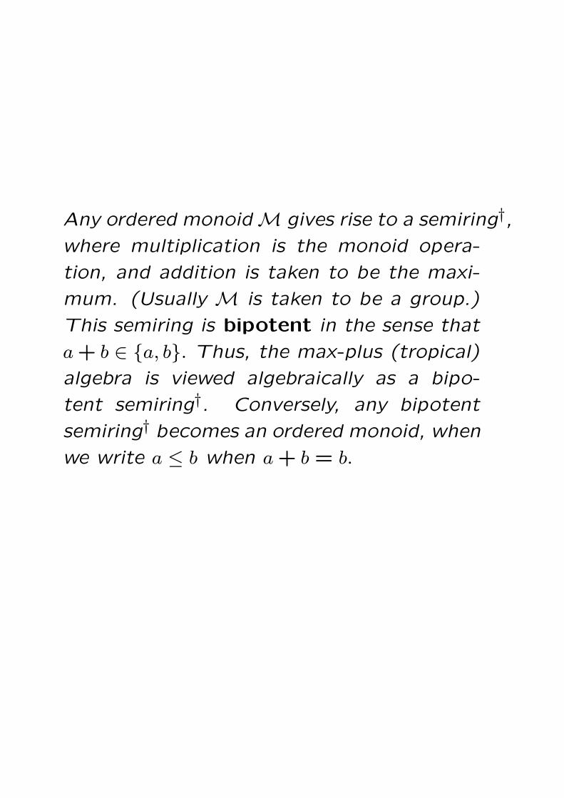
Any ordered monoid M gives rise to a semiring†,where multiplication is the monoid opera-

tion, and addition is taken to be the maxi-

mum. (Usually M is taken to be a group.)

This semiring is bipotent in the sense that

a+ b ∈ {a, b}. Thus, the max-plus (tropical)

algebra is viewed algebraically as a bipo-

tent semiring†. Conversely, any bipotent

semiring† becomes an ordered monoid, when

we write a ≤ b when a+ b = b.

§§ 4. Polynomials and matrices

For any semiring† R, one can define the

semiring† R[λ] of polynomials, namely (af-

ter adjoining 0)∑i∈N

αiλi : almost all αi = 0R

,

where polynomial addition and multiplica-

tion are defined in the familiar way:(∑i

αiλi

)(∑j

βjλj

)=∑k

( ∑i+j=k

αiβk−j

)λk.

Likewise, one can define polynomials F [Λ]

in a set of indeterminates Λ.

Any polynomial f ∈ F [λ1, . . . , λn] defines a

graph in R(n+1), whose points are

(a1, . . . , an, f(a1, . . . , an)).

The graph of a polynomial over the max-

plus algebra is a sequence of straight lines,

i.e., a polytope, and is closely related to the

Newton polytope.

Graph of λ2 +3λ+4:

In contrast to the classical algebraic

theory, different polynomials over the max-

plus algebra may have the same graph, i.e,

behave as the same function. For example,

λ2 + λ + 7 and λ2 + 7 are the same over

the max-plus algebra. There is a natural

homomorphism

Φ : R[λ1, . . . , λn] → Fun(R(n), R),

and we view each polynomial in terms of its

image in Fun(R(n), R).

Likewise, one can define the matrix semiring†

Mn(R) in the usual way.

§§ 5. Corner loci in tropicalizations

Basic fact for any valuation v: If∑

ai = 0,

then v(ai1) = v(ai2) for suitable i1, i2.

Suppose

f =∑

i∈N(n)

pi(t)λi11 · · ·λinn ,

where pi ∈ K. Write

v(f) =∑

i∈N(n)

v(pi(t))λi11 · · ·λinn .

The image under v of any root of f (over the

max-plus algebra) must be a point on which

the maximal evaluation of f on its monomi-

als is attained by at least two monomials.

This is called a corner root, and the set of

corner roots is called the corner locus.

This brings us back to the max-plus algebra,

since we are considering those monomials

taking on maximal values.

§§ 6. Kapranov’s Theorem

Example 1. f = 10t2λ3 + 9t8 has the root

λ 7→ a = − 3√

910t

2. Then

v(f) = 2λ3 +8

has the corner root v(a) = 2.

For

f = (8t5+10t2)λ3+(3t+6)λ2+(7t11+9t8)

again

v(f) = 2λ3 +0λ2 +8,

which as a function equals 2λ3+8 and again

has the corner root 2.

One can lift this to a root of f by building

up Puiseux series with lowest term − 3√

910t

2,

using valuation-theoretic methods.

Theorem 1 (Kapranov). The tropicaliza-

tion of the zero set of f coincides with the

corner locus of the tropical function.

Kapranov’s theorem leads us to evaluate poly-

nomials on the max-plus algebra. Tropical

polynomials are also viewed as piecewise lin-

ear functions f : R(n) → R; then the corner

locus is the domain of non-differentiability

of the graph of f .

Example 2. The polynomial 2x3 + 6x + 7

over the max-plus algebra has corner locus

{1,2} since

2 · 23 = 2 · 6 = 8, 6 · 1 = 7.

Its graph (rewritten in classical algebra) con-

sists of the horizontal line y = 7 up to x = 1,

at which point it switches to the line seg-

ment y = x+6 until x = 2, and then to the

line y = 3x+2.

§§ 7. Nice properties of bipotent semiring†s

• Any bipotent algebra satisfies the amaz-

ing Frobenius property:(∑ai)m

=∑

ami (1)

for any natural number m.

• Any polynomial in one indeterminate can

be factored by inspection, according to

its roots.

For example, λ4+4λ3+6λ2+5λ+3 has

corner locus {−2,−1,2,4} and factors as

(λ+4)(λ+2)(λ+ (−1))(λ+ (−2)).

§§ 8. Poor properties of bipotent semiring†s

Unfortunately, bipotent semiring†s have two

significant drawbacks:

• Bipotence does not reflect the true na-

ture of a valuation v. If v(a) = v(b) then

v(a+b) ∈ {v(a), v(b)}, so bipotence holds

in this situation, but if v(a) = v(b) we do

not know much about v(a+ b). For ex-

ample, the lowest terms in two Puiseux

series may or may not cancel when we

take their sum.

• Distinct cosets of ideals need not be

disjoint. In fact for any ideal I, given

a, b ∈ R, if we take c ∈ I large enough,

then

a+ c = c = b+ c ∈ (a+ I) ∩ (b+ I).

This complicates everything involving ho-

momorphisms and factor structures. One

does not describe homomorphisms via

kernels, but rather via congruences, which

is much more complicated.

Thus, the literature concerning the struc-

ture of max-plus semiring†s is limited. There

are remarkable theorems, but they are largely

combinatoric in nature, and often the state-

ments are hampered by the lack of a proper

language. The objective of this research is

to provide the language (and basic results)

for a framework of the structure theory.

§§ 9. The supertropical semiring†

The structure is improved by considering acover of our given ordered Abelian monoid,which we denote as R∞, rather than viewR∞ directly as a bipotent semiring†. Namely,we take a monoid surjection ν : R1 → R∞.

(Often ν is an isomorphism.) We write aν

for ν(a), for each a ∈ R1.

The disjoint union R := R1∪R∞ becomes amultiplicative monoid under the given monoidoperations on R1 and R∞, when we defineabν, aνb both to be aνbν ∈ R∞.

We extend ν to the ghost map ν : R → R∞by taking ν to be the identity on R∞. Thus,ν is a monoid projection.

We make R into a semiring† by defining

a+ b =

a for aν > bν;

b for aν < bν;

aν for aν = bν.

R so defined is called a supertropical domain†.

Another way to view multiplication is to de-

fine νi : R1 → Ri (for i ∈ {1,∞} by ν1 = 1R1

and ν∞ = ν. Then multiplication is given by

νi(a)νj(b) = νij(ab).

R∞ is a semiring† ideal of R. R1 is called

respectively the tangible submonoid of R,

and R∞ is ghost ideal also denoted as G.We could formally adjoin a zero element in a

new component R0, since this has properties

both of tangible and ghost.

Special Case: A supertropical semifield†

is a supertropical domain† for which R1 is

an Abelian group.

Examples

• R1 = (R,+), R∞ = (R,+), and ν is the

identity map (Izhakian’s original exam-

ple);

• R1 = F× (F a field), R∞ is an ordered

group, and ν : F× → R∞ is a valuation.

Note that we forget the original addition

on the field F !

The innovation: The ghost ideal R∞ is to be

treated much the same way that one would

customary treat the 0 element in commuta-

tive algebra. Towards this end, we write

a |G= b if a = b or a = b+ ghost.

(Accordingly, write a |G= 0 if a is a ghost.)

Note that for a tangible, a |G= b iff a = b.

This partial order |G=, called ghost surpasses,

is of fundamental importance in the supertrop-

ical theory, replacing equality in many analogs

of theorems from commutative algebra.

Supertropical domains† also satisfy the Frobe-

nius property

(a+ b)m = am + bm, ∀m.

A suggestive way of viewing (1) is to note

that for any m there is a semiring† endomor-

phism R → R given by f 7→ fm, reminiscent

of the Frobenius automorphism in classical

algebra. But here the Frobenius property

holds for every m. This plays an important

role in our theory, and is called character-

istic 1 in the literature.

§ 2. Semirings with ghosts

To handle polynomials and matrices directly,

we need to describe the structure slightly

more generally.

A semiring† with ghosts (R,G, ν) consists

of a semiring† R, a distinguished ideal called

the ghost ideal G, and a semiring† homo-

morphism ν : R → G such that ν2 = ν.

If (R,G, ν) is a semiring† with ghosts, then

for any set S, Fun(S,R) is also a semiring†

with ghosts, whose ghost ideal is Fun(S,G).

Bipotency fails for polynomials:

(2λ+1)+ (λ+2) = 2λ+2.

If a polynomial f = 0, then f cannot have

any zeroes in the classical sense! But here

is an alternate definition.

An n-tuple a = (a1, . . . , an) ∈ R(n) is called

a root of a polynomial f ∈ R[λ1, . . . , λn] if

f(a) |G= 0, i.e., if f(a) ∈ G.

There are two kinds of values of f =∑

hj,

where hj are monomials:

Case I At least two of the hj(a)ν are maxi-

mal (and thus equal), in this case

f(a) = hj(a)ν ∈ G.

Tangible roots in this case are just the

corner roots.

Case II There is a unique j for which hj(a)ν

is maximal in G. Then f(a) = hj(a); this

will be ghost when the coefficient of hjis ghost.

Example 3. (The tropical line) The tangi-

ble roots in D(R)[λ] of the polynomial f =

λ1 + λ2 +0 are:

(0, a) for a < 0;

(a,0) for a < 0;

(a, a) for a > 0.

The “curve” of tangible roots of f is com-

prised of three rays, all emanating from (0,0).

§§ 10. The tropical version of the algebraic

closure

A semiring† R is divisibly closed if m√a ∈ R

for each a ∈ R. There is a standard con-

struction to embed a semifield† into a divis-

ibly closed, supertropical semifield†.

Example: The divisible closure of the max-

plus semifield† Z is Q, which is closed under

taking roots of polynomials.

Theorem 1. If two polynomials agree on an

extension of a divisibly closed supertropical

semifield† R, then they already agree on R.

The proof is an application of Farkas’ the-

orem from linear inequalities!

§§ 11. Factorization

An example of an irreducible quadratic poly-

nomial:

λ2 +5νλ+7.

(although λ2 + 5νλ + 7 = (λ + 2)(la + 5).

But this is the only kind of example:

Theorem 2.Any polynomial over a divisibly

closed semifield† is the product (as a func-

tion) of linear polynomials and quadratic poly-

nomials of the form λ2+aνλ+b, where ba < a.

Unique factorization can fail, even with re-spect to equivalence as functions.

In one indeterminate:

λ4 +4νλ3 +6νλ2 +5νλ+3

= (λ2 +4νλ+2)(λ2 +2νλ+1)

= (λ2 +4νλ+2)(λ+ (−1))(λ+2)

= (λ2 +4νλ+3)(λ2 +2νλ+0).

A geometrical interpretation of these fac-torizations: The tangible root set of f isthe interval [−2,4], where −1 and 2 alsoare corner roots. The tangible root set ofany irreducible quadratic factor λ2+aνλ+ b

is the closed interval [ba, a], and the unionof these segments must correspond to theroot set of f . Different decompositions ofthe tangible root set yield different factor-izations.

The decomposition for the factorization(λ2 +4νλ+2)(λ+ (−1))(λ+2) is

[−2,4] ∪ {−1} ∪ {2},

which is the decomposition best matching

the geometric intuition.

The decompositions of the root set for the

other factorizations are respectively:

[−2,4] ∪ [−1,2]; [−1,4] ∪ [−2,2]

In two indeterminates, we have a worse sit-

uation:

(0 + λ1 + λ2)(λ1 + λ2 + λ1λ2)

= λ1 + λ2 + λ21 + λ22

+ ν(λ1λ2) + λ21λ2 + λ22λ1

= (0+ λ1)(0 + λ2)(λ1 + λ2).

But this is an instance of the important phe-

nomenon that a tropical variety can decom-

pose in several ways as the union of irre-

ducible varieties (in this case, either as a

tropical line together with a tropical conic,

or three rays).

§ 3. Supertropical matrix theory

Since −1 is not available in tropical math-

ematics, our main tool in linear algebra is

the permanent |A|, which can be defined for

any matrix A over any commutative semir-

ing. Although the permanent is not multi-

plicative in general, it is multiplicative in the

supertropical theory, in a certain sense, and

enables us to formulate many basic notions

from classical matrix theory.

Assume R = (R,G, ν) is a commutative su-

pertropical domain†.

Define the tropical determinant as∣∣∣(ai,j)∣∣∣ = ∑π∈Sn

aπ(1),1 · · · aπ(n),n. (2)

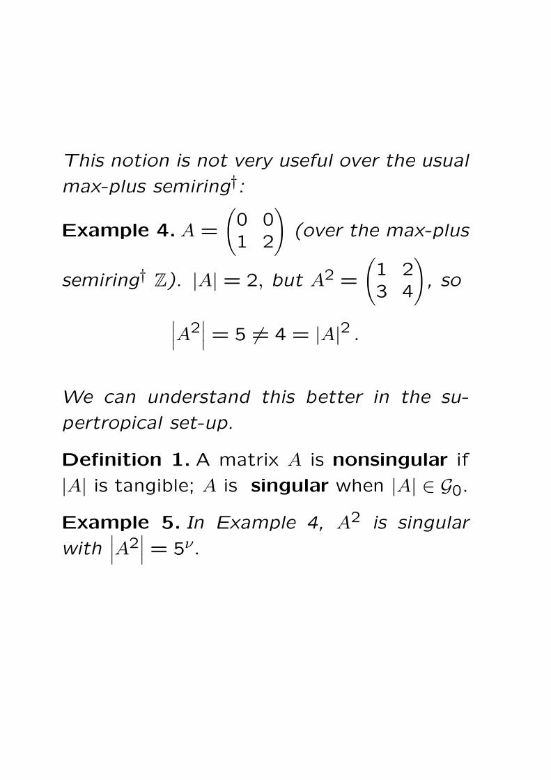
This notion is not very useful over the usual

max-plus semiring†:

Example 4.A =

(0 01 2

)(over the max-plus

semiring† Z). |A| = 2, but A2 =

(1 23 4

), so

∣∣∣A2∣∣∣ = 5 = 4 = |A|2 .

We can understand this better in the su-

pertropical set-up.

Definition 1. A matrix A is nonsingular if

|A| is tangible; A is singular when |A| ∈ G0.

Example 5. In Example 4, A2 is singular

with∣∣∣A2

∣∣∣ = 5ν.

Theorem 3. For any n× n matrices over a

supertropical semiring R, we have

|AB| |G= |A| |B| .

In particular, |AB| = |A| |B| whenever AB is

nonsingular.

Definition 2.The minor A′i,j is obtained by

deleting the i row and j column of A. The

adjoint matrix adj(A) is the transpose of

the matrix (a′i,j), where a′i,j =∣∣∣A′

i,j

∣∣∣.

Some easy calculations:

• |A| =∑n

j=1 ai,j a′i,j, ∀i.

•∑n

j=1 ai,j a′k,j |

G= 0,

∑nj=1 a

′j,i aj,k |

G= 0,

∀k = i.

• adj(AB) |G= adj(B) adj(A).

• adj(At) = adj(A)t.

Theorem 4.

1. |A adj(A)| = |A|n .

2. |adj(A)| = |A|n−1 .

The proof of equality (rather than just ghost

surpasses) follows as a direct consequence

of the celebrated theorem of Birkhoff and

Von Neumann, which states that every pos-

itive doubly stochastic n×n matrix is a con-

vex combination of at most n2 cyclic covers.

Definition 3. A quasi-identity is a multi-

plicatively idempotent matrix of tropical de-

terminant 1, equal to the identity on the

diagonal and ghost off the diagonal.

Theorem 5. For any nonsingular matrix A

over a supertropical semifield† F ,

A adj(A) = |A| IA,

for a suitable quasi-identity matrix IA.

Likewise adj(A)A = |A| I ′A, for a suitable

quasi-identity matrix I ′A. (I ′adj(A) = IA.)

The adjoint also is used to solve the matrix

equations Ax |G= v for tangible vectors x, v.

The supertropical version of the Hamilton-

Cayley theorem: The matrix A satisfies the

polynomial f ∈ R[λ] if f(A) |G= (0); i.e.,

f(A) ∈ Mn(G).

Theorem 6.Any matrix A satisfies its char-

acteristic polynomial fA = |λI +A|.

Example 6. The characteristic polynomial

fA of

A =

(4 00 1

)over F = D(R), is (λ + 4)(λ + 1) + 0 =

(λ+4)(λ+1), and indeed the vector (4,0) is

a eigenvector of A, with eigenvalue 4. How-

ever, there is no eigenvector having eigen-

value 1.

Definition 4. A vector v is a supertropi-

cal eigenvector of A, with supertropical

eigenvalue β ∈ T , if

Av |G= βv

for some m; the minimal such m is called

the multiplicity of the eigenvalue (and also

of the eigenvector).

In Example 6, (0,4) is a supertropical eigen-

vector of A having eigenvalue 1, although it

is not an eigenvector.

Theorem 7.The roots of the polynomial fAare precisely the supertropical eigenvalues

of A.

§ 4. Tropical dependence of vectors

Definition 5. A subset W ⊂ R(n) is trop-

ically dependent if there is a finite sum∑αiwi ∈ G(n)

0 , with each αi tangible; other-

wise W is called tropically independent.

Here is our hardest theorem:

Theorem 8. Suppose R is a supertropical

domain†. The following three numbers are

equal for a matrix:

• The maximum number of tropically in-

dependent rows;

• The maximum number of tropically in-

dependent columns;

• The maximum size of a square nonsin-

gular submatrix of A.

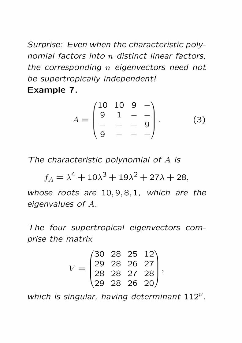
Surprise: Even when the characteristic poly-

nomial factors into n distinct linear factors,

the corresponding n eigenvectors need not

be supertropically independent!

Example 7.

A =

10 10 9 −9 1 − −− − − 99 − − −

. (3)

The characteristic polynomial of A is

fA = λ4 +10λ3 +19λ2 +27λ+28,

whose roots are 10,9,8,1, which are the

eigenvalues of A.

The four supertropical eigenvectors com-

prise the matrix

V =

30 28 25 1229 28 26 2728 28 27 2829 28 26 20

,

which is singular, having determinant 112ν.

This difficulty is resolved by passing to asymp-

totics, i.e., high enough powers of A. In

contrast to the classical case, a power of

a nonsingular n × n matrix can be singular

(and even ghost).

§ 5. The resultant

We now have all the tools at our disposal to

define the supertropical resultant, in terms

of Sylvester matrices, which enables us to

determine when two polynomials have a com-

mon root and yields an algebraic proof of a

version of Bezout’s theorem.

§ 6. Layered structure

In order to handle multiple roots and deriva-

tives, we need to consider multiple ghost

layers, “sorted” over an ordered semiring L

all of whose elements are presumed positive

or 0.

Our main objectives:

• Introduce the refined layered structureand develop its basic properties, in anal-ogy with the supertropical theory devel-oped previously. This includes a descrip-tion of polynomials and their behavior asfunctions.

• Indicate how the refined structure ex-tends the scope of the supertropical the-ory, as well as the max-plus theory. Forexample, we can treat multiple roots bymeans of layers.

• Show how certain supertropical proofsactually become more natural in this the-ory.

• Relate these various concepts to notionsalready existing in the tropical literature.

The familiar max-plus algebra is recovered

by taking L = {1}, whereas the standard su-

pertropical structure is obtained when L =

{1,∞}. Other useful choices of L include

{1,2,∞}, N, Q>0, R>0, Q, and R. The 1-

layer is a multiplicative monoid correspond-

ing to the tangible elements in the stan-

dard supertropical theory, and the ℓ-layers

for ℓ > 1 correspond to the ghosts in the

standard supertropical theory.

Unique factorization fails in the standard su-

pertropical theory. Taking L = N yields

enough refinement to permit us to utilize

some tools of mathematical analysis. Tak-

ing L = Q>0 permits one to factor poly-

nomials in one indeterminate into primary

factors, and “almost” restores unique fac-

torization in one indeterminate. The sticky

point here is polynomials with a single root,

which we call primary; these have the form∑i

aiλd−i.

(Unique factorization in several indetermi-

nates still fails in certain situations, but be-

cause certain tropical hypersurfaces can be

decomposed non-uniquely).

Our main construction:

Suppose we are given a cancellative ordered

monoid M. For any semiring† L we define

the semiring† R(L,M) to be set-theoretically

L ×M, where for k, ℓ ∈ L, and a, b ∈ M, we

define multiplication componentwise, i.e.,

(k, a) · (ℓ, b) = (kℓ, ab), (4)

and addition from the rules:

(k, a) + (ℓ, b) =

(k, a) if a > b,

(ℓ, b) if a < b,

(k+ℓ, a) if a = b.

(5)

Here, L measures the ghost level. Adding

two elements of the value in M raises the

ghost level accordingly. We write [k]a for

(k, a), and define the map s : R → L by

s( [k]a ) = k, for any a ∈ M, k ∈ L.

R := R(L,G) is a semiring†.

§§ 12. Layered varieties

Here are the main geometric definitions.

Definition 6. An element a ∈ S is a corner

root of a polynomial f if f(a) = h(a) for

each monomial h of f.

(In other words, we need at least two mono-

mials to attain the appropriate ghost level

of f(a).)

The corner locus Zcorn(I) of I ⊂ R[Λ] is

the set of simultaneous corner roots of the

functions in I. Any such corner locus will

also be called an (affine) layered variety.

The (affine) coordinate semiring† of a lay-

ered variety Z is R[Λ] ∩ Fun(Z,R).

§§ 13.The component topology

Definition 7.Write f =∑

i fi for i = (i1, . . . , in),

a sum of monomials.

Define the components Df,i of f to be

Df,i := {a ∈ S : f(a) = fi(a)}.

We write f≼comp,layI for I ⊆ F [λ1, . . . , λn],

if for every essential monomial fi of f there

is g ∈ I (depending on Df,i) with f ≼Df,ig

and ϑf(a) ≥ ϑg(a).

For I ⊆ F [Λ], define

f |L= g iff either

f = g + h with h s(g)-ghost,

f = g,

or

f ∼=ν g with f s(g)-ghost,

and

Lay√I = {f ∈ I : fk |L= g for some g ∈ I}.

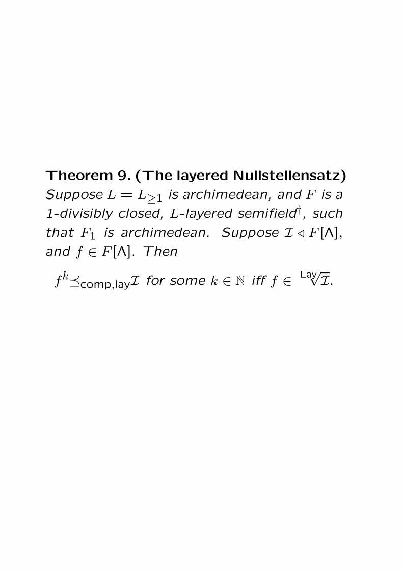
Theorem 9. (The layered Nullstellensatz)

Suppose L = L≥1 is archimedean, and F is a

1-divisibly closed, L-layered semifield†, suchthat F1 is archimedean. Suppose I ▹ F [Λ],

and f ∈ F [Λ]. Then

fk≼comp,layI for some k ∈ N iff f ∈ Lay√I.

HAPPY BIRTHDAY, DAVID