This article was downloaded by: [Michigan State University]On: 04 October 2013, At: 08:04Publisher: Taylor & FrancisInforma Ltd Registered in England and Wales Registered Number: 1072954 Registeredoffice: Mortimer House, 37-41 Mortimer Street, London W1T 3JH, UK

Journal of Statistical Computation andSimulationPublication details, including instructions for authors andsubscription information:http://www.tandfonline.com/loi/gscs20

An alernative test for normality basedon normalized spacingsLing. Chen a & Samuel S. Shapiro aa Department of Statistics, Florida International University,Published online: 20 Mar 2007.

To cite this article: Ling. Chen & Samuel S. Shapiro (1995) An alernative test for normality basedon normalized spacings, Journal of Statistical Computation and Simulation, 53:3-4, 269-287, DOI:10.1080/00949659508811711

To link to this article: http://dx.doi.org/10.1080/00949659508811711

PLEASE SCROLL DOWN FOR ARTICLE

Taylor & Francis makes every effort to ensure the accuracy of all the information (the“Content”) contained in the publications on our platform. However, Taylor & Francis,our agents, and our licensors make no representations or warranties whatsoever as tothe accuracy, completeness, or suitability for any purpose of the Content. Any opinionsand views expressed in this publication are the opinions and views of the authors,and are not the views of or endorsed by Taylor & Francis. The accuracy of the Contentshould not be relied upon and should be independently verified with primary sourcesof information. Taylor and Francis shall not be liable for any losses, actions, claims,proceedings, demands, costs, expenses, damages, and other liabilities whatsoeveror howsoever caused arising directly or indirectly in connection with, in relation to orarising out of the use of the Content.

This article may be used for research, teaching, and private study purposes. Anysubstantial or systematic reproduction, redistribution, reselling, loan, sub-licensing,systematic supply, or distribution in any form to anyone is expressly forbidden. Terms &Conditions of access and use can be found at http://www.tandfonline.com/page/terms-and-conditions

J. Statist. Comput. Simul., 1995, Vol. 53, pp. 269-287 Reprints available directly from the publisher Photocopying permitted by license only

% 1995 OPA (Overseas Publishers Association) Amsterdam B.V. Published in The Netherlands under license by Gordon and Breach Science Publishers SA

Printed in Malaysia

AN ALTERNATIVE TEST FOR NORMALITY BASED ON NORMALIZED SPACINGS

LING CHEN and SAMUEL S. SHAPIRO

Department of Statistics, Florida International University

(Receiued June 20,1994; injinal form July 7, 1995)

The Shapiro-Wilk statistic and its tnodifications are widely used for assessing the assumption that a sample was drawn from a normal distribution. Many of the modifications simplified the calculation of the test statistic but resulted in a loss of power. In this paper, we propose an alternative statistic for testing normality which is easy to compute and has power comparable or superior to the original W test.

KEY WORDS: BLUE weights; Covariance matrix; Eigenvalues; Normalized spacing; Normality tests.

1. INTRODUCTION

Shapiro and Wilk (1965) proposed the following test statistic for assessing the nor- mality assumption:

where x, is the ith order statistic from a sample of size n,

m ' T 1 a' =(a1, ..., a,) = -- (m'V- lv- l m ) l / 2 '

and m, V are the vector of expected values and covariance matrix of the order statistics of the standard normal distribution.

Since the values of V were not really available for large sample sizes, Shapiro and Francia (1972) introduced the modified W-statistic by substituting the identity matrix Z for V-'. The approximate W' test for normality was defined as

W' = (m 'Y)

(m'm)xy= l ( x - Y)*'

It was reported in Shapiro and Francia's paper that the W' test appeared to be more sensitive to non-normality than the W test when the alternative distribution was continuous and symmetric with a high fourth moment (as compared to the normal distribution), when it was near normal and when it was discrete and skewed. The

Dow

nloa

ded

by [

Mic

higa

n St

ate

Uni

vers

ity]

at 0

8:04

04

Oct

ober

201

3

270 L. CHEN AND S. S. SHAPIRO

two tests appeared to be equivalent for alternative distributions which were continu- ous and asymmetric with high fourth moment and discrete and symmetric. However the Wtest was superior to the W' test for many other alternative distributions.

Weisberg and Bingham (1975) proposed modifying W' by replacing the elements of m by H ((i - 3/8)/(n + 1/4)), where H is the inverse of the N (0,l) distribution function. The resulting statistic has the advantage over Wand W' that, for machine computation, no storage of constants is required when a routine for the inverse standard normal distribution is available.

Ryan and Joiner (1973) and Filliben (1975) interpreted W' as the square of the correlation coefficient associated with a normal probability plot and Filliben pro- posed

as an alternate version of the Shapiro-Wilk statistic, where Mi is the median of the ith order statistic from a standard normal sample of size n. Filliben compared his test to Wand W' with a significance level 0.05 and n = 20,50. The results showed that Filliben test is comparable to W' test but not to the Wtest. While it is better than the Wtest for symmetric alternatives with longer tails than the normal distribu- tion, the Wtest is much better than the Filliben test for symmetric alternatives with shorter tails than the normal distribution and is better than the Filliben test for skewed alternatives.

De Wet and Venter (1972,1973) obtained the asymptotic distribution of the modi- fied Shapiro-Wilk statistic r, which used Hi = H(i/(n + 1)) instead of Mi in r,.

Verrill and Johnson (1987) proved the asymptotic equivalence of Shapiro-Francia, Filliben, Weisberg-Bingham and de Wet-Venter versions of the modified Shapiro- Wilk statistic. For studying asymptotic power, they suggested using contiguous alternatives and pointed out that by the definition of contiguity, the equivalence of the statistics would continue to hold.

A comparison of these modified versions of the Wtest shows that while these tests reduce the computational effort their power of the test is lower than W for many alternative distributions, especially, when the sample size is small.

Royston (1992) proposed a new approximation for the coefficients required to calculate the W test and proposed a normalizing transformation for the Wstatistic so that the p-value of the test could be obtained from normal tables. (This is denoted Z in this paper.)

In this paper, we propose an alternative to these tests. The test statistic is based on the ratio of two estimators of the scale parameter of a normal distribution, one of which is based on the normalized spacings. The test statistic uses the same approach as Weisberg and Bingham did in the modified W' but its power is comparable or superior to the original W test. Section 2 introduces the suggested procedure and describes some of its properties, Section 3 give a comparison of its power with U( WH, and Z and Section 4 gives a discussion of the relationship among the four tests. An illustrative example is given in Section 5. The last section has the conclusions.

Dow

nloa

ded

by [

Mic

higa

n St

ate

Uni

vers

ity]

at 0

8:04

04

Oct

ober

201

3

A N ALTERNATIVE TEST 271

2. THE Q H * TEST FOR NORMALITY

The alternate versions of the W test use only information concerning the expecta- tions of normal order statistics and no information on correlation. This results in procedures with lower power for many alternatives. We shall introduce a new procedure which is based on normalized spacings and has the advantage of being easy to compute while having comparable or superior power to the original W test.

2.1. Motivation

The motivation of the original W was based on an analysis of variance viewpoint which compared the squared slope of the probability plot regression line, which under the normality hypothesis is an estimate of the population variance multiplied by a constant, with the total sum of squares about the mean, which is an estimate of the variance (up to a constant) independent of the null hypothesis. For ease of notion, let X,,X,, . . .,X, be the order statistics from N(0, 1) and mi = E(Xi). Similar- ly, let Yi be the order statistics from N(p,a2). Thus,

where E~ are the error terms. Since the ci are correlated, Shapiro and Wilk (1965) used generalized least squares (Aitken, 1935; Lloyd, 1952) to get a BLUE estimator for a. Subsequently (Shapiro and Francia, [1972]), using the suggestion of Gupta (1952) that for large samples, the observtions {y,) may be treated as if they were independent, the identity matrix I was substituted for V -' in the estimation of the slope of the regression line, and this resulted in the W' test.

Suppose F (x) is a completely specified continuous distribution function, and let Y have a distribution function G(y), where Y= p + OX, thus p and a are location and scale parameters in G(y). If Y, c Y2 < ... < Y, are the order statistics of a random sample from G (y), the Yi can be represented as T = p + ax , , where Xi is an ordered random sample from F (x). Suppose mi = E(Xi); since F (x) is completely specified, mi can be calculated. The spacings between the E;: are defined by y+ , - Y, i = 1,2,. . . n- 1 and the normalized spacings are

When the Y-sample comes from an exponential distribution

the quantity mi+, -mi in the denominator of Zi is l/(n - i), and Zi are a random sample from G E ( . ) above.

For general G (y), the normalized spacings are not a random exponential sample, even asymptotically. A property of the normalized spacings is that, as n -t a, for any regular parent population G(y) for X and for "sufficiently separate" indices k and 1, Y , and I; converge to independent exponentials, as k, and I , n -, a, and k/n+p and l/n+q, with both p and q in (0,l) and p # q; see Pyke (1965,p.407). Normalized spacings provide useful tests of fit for many suitably regular continuous

Dow

nloa

ded

by [

Mic

higa

n St

ate

Uni

vers

ity]

at 0

8:04

04

Oct

ober

201

3

272 L. CHEN AND S. S. SHAPIRO

distributions. (See Lockhart et al. [1985]) This motivated us to consider a regression - 7 on mi+ -mi.

From (2), we have

Hence,

Let

and

we have

Minimizing El; results in

It is easy to see that B is an unbiased estimator of a. Since 4 are correlated, it is not a BLUE estimator. But, from the properties of normalized spacings, the correla- tions among them should be less than that among 7's. It is interesting that this is true for samples from a standard normal distribution even for small sample sizes.

Table 1 shows correlation matrices of 7 and Zi for sample sizes n = 4 and 5 from which the reduction of the correlations can be seen.

Therefore, using the basic rationale of the W test, we considered a statistic as follows:

1 n - 1 7 + l - y C ( n - 1) s i = l mi+l -mi'

Table 1 Comparison of co~relation matrices of Yi and Zi. The upper triangle is for Yi and the lower triangle is for Zi.

Dow

nloa

ded

by [

Mic

higa

n St

ate

Uni

vers

ity]

at 0

8:04

04

Oct

ober

201

3

AN ALTERNATIVE TEST 273

where S = (c!= ,(q - P)'/(n - 1)) ' I 2 . In order to simplify the computations, the expected values of the order statistics from the standard normal distribution were replaced by Hi, similar to Weisberg and Bingham's W' test. Thus, we have the following new test statistic:

where Hi = a- ' ( ( i - 3/8)/(n + 114)) and @-I( . ) is the inverse of the standard normal distribution.

When the null hypothesis is true, the distribution of QH will have a mean close to one. Deviations from normality will shift the distribution toward its lower bound and hence a lower tailed test is used.

Analytical properties of QH are given in Appendix A.

2.2. Approximating the Distribution of QH

The distribution of QH under the null hypothesis was investigated empirically. Standard normal samples were obtained using CMLIB. Repeated values of QH were computed for n = 3(1)50,60,80,100,150,250,500,1000,2000 and the empirical per- centage points determined for each value of n. The number of samples m = 100,000 was employed. Figure 1 gives the empirical c.d.f.'s for values of n = 5,10,20,35 and 50. Figure 2 gives a plot of the 0.5, 1,2.5,5,50,95, and 99 empirical percentage points of QH for n = 3(1)50. From Figure 1 and 2, it is seen that the distribution of QH is negatively skewed. The variance of the distribution decreases rapidly as the sample size increases.

2.3. A New Test Statistic for Normality-QH*

In order to eliminate the need for tables of percentiles, we define

QH* = , /n ( l - QH). (5)

Thus QH* is an upper-tailed test. Regression equations were fit to selected upper percentiles of QH* as a function of sample size. This was done for 16 percentiles: 0.001,0.005 (0.005) 0.05 (0.01) 0.10. The regression equations are given in Table 2.

The fitted functions in Table 2 provide good approximations to the sampling results, the average R 2 of the 16 regression fits was 0.9974937 and the average residual mean squares was 3.5136391E-06 (These are not independent of each other). With 95% probability the simulation error in terms of percentages is

Smoothed upper tail percentage points of QH* are given in Appendix B. Fortran subroutines for upper tail percentage points of QH* are given in Appendix C.

Dow

nloa

ded

by [

Mic

higa

n St

ate

Uni

vers

ity]

at 0

8:04

04

Oct

ober

201

3

274 L. CHEN AND S. S. SHAPIRO

an

Figure 1 Empirical c.d.f. of QH for n = 5, 10, 15, 20, 35, 50.

10 20 30 40 50

Sample size, n

Figure 2 Selected expirical percentage points of QH, n = 3(1)50.

3. MONTE CARL0 POWER STUDY

3.1. Description of Monte Carlo Experiment

The power of QH* was compared to the Shapiro-Wilk Wand Weisberg-Bingham tests the latter denoted by WH in this paper. The Wused in the study is the original Wtest using Royston's (1992) approximations for the a,. Also included was Royston (1992) transformed Wwhich results in a Z test for normality. Since Royston did not include any power comparisons for the Z test in his paper, this was included in this study. The following alternative distributions were selected: uniform(O,l), Cauchy,

Dow

nloa

ded

by [

Mic

higa

n St

ate

Uni

vers

ity]

at 0

8:04

04

Oct

ober

201

3

A N ALTERNATIVE TEST

Table 2 Regression equations Q ~ E =yo + + y,n-'I3 + y,n-"' for 1 0 G n G2000.

chi squared, lognormal, non-central t (denoted T(.,.)), logistic, La Place, beta, binomial and Poisson. Monte Carlo samples of size 100,000 were used to calculate the critical points for WH. The critical points of Wand Z were obtained from Table 2 in Royston (1992). The critical points for QH* were calculated based on the regression equations in Table 2. A total of 100,000 runs were used to calculate the power of each procedure for each alternative and each sample size (n = 20,40,60). Each test was run at significance levels of 0.05, and 0.01. 3.2. Computational Techniques

Fortran 77 was used for all Monte Carlo studies. CMLIB random generating func- tion UNI and RNOR were used to generate pseudo uniform and normal random numbers respectively. The other random variates were created by using the methods given in Devroye (1986). All programs were run on VMS Dec-Alpha-7620.

3.3. Power Comparisons

The results of the study of the power of QH*, W, Z and WH for three sample sizes (20,40, and 60), two levels of test (0.01 and 0.05) and 14 alternative distributions are shown in Table 3. The table gives the power of each procedure for the stated alternative. Thus one can see that the relative power ranking of any procedure depended on the alternative distribution. For example the power of QH* was higher than W for the uniform and beta(2, 1) distributions but was less for the Cauchy and Logistic distributions. In order to summarize these comparisons Tables 4 and 5 are given. In Table 4 the results of 252 (14 alternatives x 3 procedures x 2 test levels x 3 sample sizes) comparisons of QH* with the other procedures are given. Three

Dow

nloa

ded

by [

Mic

higa

n St

ate

Uni

vers

ity]

at 0

8:04

04

Oct

ober

201

3

276 L. CHEN AND S. S. SHAPIRO

Table 3 Empirical power for 1% and 5% tests for selected alternative distributions. Here p:I2 and p2 denote the standardized measure of skewness and kurtosis of a distribution, respectively.

Population JB; 82 n cc level title

0.01 0.05

W Z QH* WH W Z QH* WH

Uniform

Cauchy

x2(1)

x 2(2)

x 2(4)

x2(l0)

Lognormal (0,l)

T (5J.4)

T(10,3.1)

Logistic

La Place

Beta(2,l)

B(4,0.5)

Poisson (1)

Dow

nloa

ded

by [

Mic

higa

n St

ate

Uni

vers

ity]

at 0

8:04

04

Oct

ober

201

3

AN ALTERNATIVE TEST

Table 4 Out of 14 alternatives, table shows the numbers of times which power of QH* is greater than, equal to, less than that of its competitors.

QH* us W QH* usZ QH* us W H > = < > = < > = <

n = 20 11 1 2 11 1 2 11 0 3 n = 40 7 3 4 7 3 4 9 2 3 n = 60 5 6 3 5 6 3 7 4 3

a = .05 QH* us W QH* vsZ QH* us WH > = < > = < > = <

counts are given for each test, sample size and test level; the number of times the power of QH* was greater than, equal to and less than the competitor test. Thus 66 out of 84 times the power of QH* was equal to or better than I/t: 66 times equal to or better than Z and 66 times equal to or better than WH. While these comparison ignore the magnitude of the differences it does indicate that QN* is probably better than the three competitors for these alternatives. Detailed analysis of the data in Table 3 confirms this supposition. It should be noted that the W; Z and QH* procedures all have lower powers than the WH test for the Cauchy, Logistic and La Place alterna- tives, but QH* is more powerful than WH and even I/t: Z for the other alternatives, especially when n = 20. In Table 5 the power comparisons of QH* with Z and WH are arrayed in a two way table according to the skewness and kurtosis of the alterna- tive distribution. The entries in the table show the number of alternative distributions

Table 5 Out of 13 alternatives, table shows the numbers of times where power of QH* is greater than or equal to that of its com- petitors in the comparison, where 2:2 means that the power of QH* is greater than or equal to that of its competitors in each of two comparisons. There are two columns and three rows in each cell. The first column is for a = 0.01 and the second column is for tt = 0.05. The first row is for n = 20, the second row is for n = 40 and the third row is for n = 60.

QH* us Z QH* us W H

Dow

nloa

ded

by [

Mic

higa

n St

ate

Uni

vers

ity]

at 0

8:04

04

Oct

ober

201

3

278 L. CHEN AND S. S. SHAPIRO

for which QH* had a power equal to or greater than the competitor and this is given for each of the three sample sizes and two test levels. Thus the fourth entry in the first row, 3:3, indicates that for sample size 20 and a test level of 0.05 QH* had a power equal to or greater than Z for all three alternatives which had 1/BT # 0 (skewed alternatives) and f i , < 3. Review of the table indicates that the QH* procedure is good or better than both Z and WH for three of the four groupings of alternatives and is poorer for the symmetric alternatives with &values equal to or greater than three.

4. FURTHER DISCUSSION O F THE RELATIONS AMONG W WH AND Q H *

In the power comparison, it can be seen that the performance of QH* is better than Wand WH, even though both Q H * and WH treat the error terms in the regression as uncorrelated to get the estimator for the scale parameter. Further investigations of the relationships among the three tests were done by first comparing the eigen- values of the covariance matrix of Zi in Section 2.1 with those of x. Tietjen, Kahaner and Beckman's table (1977) was used to obtain the covariances of the normal order statistics. The algorithms NSCORl of Royston (1982) with the covariances of the normal order statistics were used to calculate the covariance matrix of Zi. The S program was used to find the eigenvalues. Table 6 shows the comparison of some statistics of the eigenvalues for sample sizes n = 10,20, 30 and 40. Note that the Euclidean distance of a symmetric matrix to the identity matrix is ED = d m , where ,Ii are eigenvalues of the symmetric matrix. From Table 6, it is easy to see that the EDs of the covariance matrices of Zi to the identity matrix is much smaller than those of y. This suggests that the covariance matrix of Zi is far closer to the identity matrix than that of and gives an explanation of why WH departs more from Wand why QH* has higher power than WH.

A comparison can be made by transforming Q H into the same form as &'by letting di = c i / m i = 1,2,...,n, where ci are defined in equation (A3) and (A4) in Appendix A and then defining

Table 6 Some summary statistics of eigenvalues of y and Zi. Here ED is the Euclidean distance of the covariance matrix to the identity matrix.

- -

Minimum Q, Median Q, Maximum ED

Dow

nloa

ded

by [

Mic

higa

n St

ate

Uni

vers

ity]

at 0

8:04

04

Oct

ober

201

3

A N ALTERNATIVE TEST

Note that WH can be written as

where zi = ( ~ y = , ~ , ? ) - l / ~ H ~ , i = l,...,n . Thus the only difference among W WH and RH is the weights of the order statistics in the nu_merators. For sample sizes n = 3(1)50, the correlations between di and a , and between di and ai were calculated, where ai are the BLUE weights used in W It was found that all correlations of the BLUE weights with zi are greater than 0.9999, while most correlations of the BLUE weights with di are less than 0.999. The ratio of the average sum of squared difference between BLUE and di to the average sum of squared difference between BLUE and Ji less than 20% except for n =3,4, and 5, which are 0.6667,0.65151 and 0.29885 respectively. Figure 3 shows the

Figure 3 Camparison of a,.

-2 -1 0 1 2

Guanb'es of Standard Nwmal

Figure 4 Q - Q plot of SiO,.

Dow

nloa

ded

by [

Mic

higa

n St

ate

Uni

vers

ity]

at 0

8:04

04

Oct

ober

201

3

280 L. CHEN AND S. S. SHAPIRO

Table 7 SiO, content, percent by weight, of plutonic rocks of the Alaska-Aleutian Range batholith (Merrill pass sequence).

scatter plots d , - a, vs i and Zi - a, vs i when n = 10. This figure shows how the weights used in R H and WH depart from the BLUE weights ai.

In summary there is a close relationship between QH and Wand the simplicity in the calculation of QH makes QH* an attractive alternative.

5. AN EXAMPLE

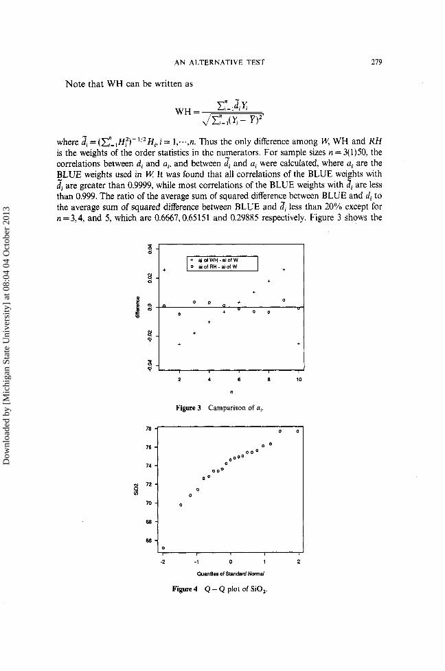
The data shown in the Table 7 are part of a larger set of data reported by Reed and Lanphere (1974). The entries in the table represent the SiO, content of plutonic rock samples taken from the Alaska-Aleutian Range batholith.

Figure 4 is the Q-Q plot of the sample against the standard normal quantiles. Prior to further analysis a test of the normality hypothesis was run. The first step in the computation of QH* is to order the data from smallest to

largest, y, < y, < ... < y,. Next the values of y,,, - y , Hi+, - Hi and S are computed.

H z - H I = H z , - H z , = 0.460291, H , - H z = H z , - H I , = 0.271697,

. a , H l o - H , = H I , - H I , = 0.119916, H I , - H l o = H I , - H l l ~0.118234,

S = 2.848382,

Substitution in (5) yields QH* = 0.074103. Using the regression estimate of the percentile with n = 21 yields QH;,,, =

0.04991. Since the value of QH* is greater than this value, the normal hypothesis is rejected at 0.05 level of significance. By using linear interpolation between two percentiles, the p-value of the QH* is approximately equal to 0.0319.

In this case, W= 0.894972 with the p-value = 0.0254 (using SAS program); Roston's Z = 1.891082 with the p-value = 0.0294; and WH = 0.940182 with p- value = 0.0265.

6. CONCLUSIONS

Since 1965, many statisticians have worked on the subject of testing for normality. There are many versions of the W' test, but none of them is comparable in power to the W test, which is probably the most widely used procedure and is included in SAS and other major statistical packages. Procedures such as Filliben's have been proposed to eliminate the need for tables of constants for the W test. Extension to higher sample sizes and elimination of tables was proposed by Royston (1992), where an approximation to W which uses a regression relationship for the a,'s and a

Dow

nloa

ded

by [

Mic

higa

n St

ate

Uni

vers

ity]

at 0

8:04

04

Oct

ober

201

3

AN ALTERNATIVE TEST 28 1

transformation for Ware given. This article has proposed a new test statistic QH* for testing the normality which requires no tables of constants and can be easily calculated if a routine for computing the inverse normal function is available. Re- gression equations are given so that the percentiles of the test statistic can be easily obtained. And the p-value of the test can be approximated by linear interpolation between two percentiles. This procedure uses the same information as Weisberg and Bingham's W' (WH). A power study indicated that the new procedure is more powerful than that suggested previously by Weisberg and Bingham for most cases studied and has a slight edge over Royston's approximation of W. The QH* can be easily changed to RH. The close relationship between di and ai indicates that the transformation made by Royston (1992) and the method for treating the ties in data by Royston (1989) could be similarly applied to RH. Due to the simplicity in obtaining QH*, it provides a handy tool for the statistical practitioner.

Acknowledgements

The authors would like to acknowledge two anonymous referees for their helpful comments znd sugges- tions which led to an improved presentation.

APPENDIX A

The statistic QH has the following analytical properties.

1. QH is scale and origin invariant. The distribution of QH depends only on the sample size n, for samples from a normal distribution.

2. QH is statistically independent of S2 and P for samples from a normal distribu- tion. This follows from the Basu theorem (Lehmann [1983]). As a result

for any r, where Zi, i = 1 ,..., n, are the order statistics from N(0,l). 3. The minimum value of QH is

This can be shown by using the fact that the statistic is origin and scale invariant, which allows the setting of XI=, % = 0 and

and then finding the minimum by maximizing c!=, Y? subject to these constraints. Under the constraints, the test statistic (4) can be written as

1 Q H =

{(n - 1) X:= x2} lI2'

Using the same argument that appears in Shapiro and Wilk (1965), the maximum of x:=, T2 in the constrained space must occur at one of the (n - 1) vertices of

Dow

nloa

ded

by [

Mic

higa

n St

ate

Uni

vers

ity]

at 0

8:04

04

Oct

ober

201

3

282 L. CHEN AND S. S. SHAPIRO

the region. The n - 1 vertices are: y, = y2 = = y, = - (n - k)(Hk+, - Hk)/n, and y,,, = ... = y, = k(H,+, - Hk)/n, for k = 1,2, ..., n - 1. These can be enumerated and checked; the maximum of c:=, K2 occurs when k = 1 or n - 1, that is,

Substitution of the maximum value in (Al) gives the stated minimum. It is also apparent that QHm, + 0 as n goes to infinity since the difference H, - H, - , changes slowly as a function of n. This can be shown by using the mean value theorem, since

where (n - 11/8)/(n + 114) < 4: < (n - 3/8)/(n + 1/4), and H(t) = W1(t) . Since

taking logs, we have H2(t) = 0(- log{t(l -t))) for t+ 0, l . Hence

Hf(t) = O({t(l - t ) ) - '[- log(t(1 - t)}] - "2).

Note that ( + 1 as n - a . Thus H,- H,-, = ~({log(n)}-~ '*) . 4. The maximum value of QH can be shown to be

where the ci are defined below. The coefficients ci of Yi+, - Y , are symmetrical about zero due to symmetry of the normal distribution and are increasing in i. Every term in the summation except Y, and Y, appears twice. We define

C, = -C 1

1 = Hn-Hn-1

and

Using this notation and setting cE, Y;. = 0 as above

1 ci K QH=

{(n - 1)

Thus using the same argument in Shapiro and Wilk (1965), the equation (A2) holds. 5. The statistic QH is used as a lower tail test to assess the normality hypothesis.

It can be shown empirically that when the expected value of the order statistics is substituted for the data, the value of QH is close to the maximum value given in (A2). Since the expected values represent an "ideal sample" from the normal, then values of the statistic for samples from non-normal distribution will result in lower values. This property is similar to that of the W test.

Dow

nloa

ded

by [

Mic

higa

n St

ate

Uni

vers

ity]

at 0

8:04

04

Oct

ober

201

3

A N ALTERNATIVE TEST

APPENDIX B

Table 1 Percentage points of the QH* test for n = 10(1)50, ..., 2000 (part 1).

Dow

nloa

ded

by [

Mic

higa

n St

ate

Uni

vers

ity]

at 0

8:04

04

Oct

ober

201

3

284 L. CHEN AND S. S. SHAPIRO

Table 2 Percentage points of the Q H* test for n = lO(l)5O, ..., 2000 (part 2 )

Dow

nloa

ded

by [

Mic

higa

n St

ate

Uni

vers

ity]

at 0

8:04

04

Oct

ober

201

3

APPENDIX C

S t r u c t u r e

s u b r o u t i n e q h s t a r l (x , n, h, q h s t a r , p q h s t a r , i f l a g , i f a u l t ) Formal p a r a m e t e r s x R e a l a r r a y ( n ) i n p u t : a s c e n d i n g o r d e r e d sample v a l u e s n I n t e g e r i n p u t : sample s i z e n=10, . . . , 2 , 0 0 0 h R e a l a r r a y ( n ) i n p u t : H ( ( i - 3 / 8 ) l ( n + 1 / 4 ) 1 , i=l, . . , n q h s t a r R e a l o u t p u t : QH* s t a t i s t i c p q h s t a r R e a l o u t p u t : a p p r o x i m a t e p - v a l u e o f t h e QH* t e s t i f l a g I n t e g e r o u t p u t : p - v a l u e i n d i c a t o r , e q u a l t o

2 i f p -va lue > 0 .1 1 i f p -va lue < 0 .001 0 o t h e r w i s e

i f a u l t I n t e g e r o u t p u t : f a u l t i n d i c a t o r , e q u a l t o 3 i f x i s no t i n a s c e n d i n g o r d e r 2 i f n < 1 0 1 i f n > 2 ,000 0 o t h e r w i s e

s u b r o u t i n e p v a l u e (qhstar,n,pqhstar,iflag) Formal p a r a m e t e r s q h s t a r R e a l i n p u t : QH* s t a t i s t i c n I n t e g e r i n p u t : sample s i z e , n-10, . . . , 2 , 0 0 0 p q h s t a r R e a l o u t p u t : a p p r o x i m a t e p -va lue o f t h e QH* t e s t i f l a g I n t e g e r o u t p u t : p -va lue i n d i c a t o r , e q u a l t o

2 i f p -va lue > 0 . 1 1 i f p -va lue < 0.001 0 o t h e r w i s e

Note: The s u b r o u t i n e p v a l u e i s c a l l e d i n s i d e o f t h e s u b r o u t i n e q h s t a r l .

s u b r o u t i n e q h s t a r l (x , n , h, qhstar,pqhstar,if lag,ifault) i n t e g e r i , n , n l , i f l a g , i f a u l t r e a l h ( n ) , p q h s t a r , f n , x s , x s s q , x h ( n ) , s x h , q h s t a r , x ( n ) , f n 1 , s

check f o r i n p u t e r r o r s

i f a u l t = l i f ( n . g t .2000) r e t u r n i f a u l t = 2 i f ( n . l t . l o ) r e t u r n nl-n-1 i f a u l t = 3 d o i=l, n l

i f ( x ( i + l ) . lt .x (i) ) r e t u r n enddo

c a l c u l a t e QH*

f n - f l o a t ( n ) f n l = f l o a t ( n l ) xs=o . 0 xssq-0 . o d o 1 0 i = l , n

xs=xs+x (i) xssq=xssq+x (i) *x ( i )

c o n t i n u e s = x s s q - x s * x s / f n sxh=O. 0 do 20 i -1 , r i l

x h ( i ) = ( x ( i + l ) -x ( i ) ) / ( h ( i + l ) - h ( i ) ) sxh-sxh+xh ( i )

c o n t i n u e q h s t a r - s q r t ( f n ) * ( 1 . 0 - s x h / s q r t (s) / s q r t ( f n l ) )

Dow

nloa

ded

by [

Mic

higa

n St

ate

Uni

vers

ity]

at 0

8:04

04

Oct

ober

201

3

286 L. CHEN AND S. S. SHAPIRO

calculate approximate p-value of the QH* test

call pvalue (qhstar, n, pqhstarfllag)

return end

subroutine pvalue (qhstar, n, pqhstar,iflag) integer i, n, iflag real qhstar,pqhstar,p(l6) ,coefO (16) ,coefl(l6) ,

$ coef2 (16) ,coef3 (16) ,qqhstar(l6), fn data p/0.001,0.005,0.010IO.O15rO.O2OIO.O25,0.O3OlO.O35~

$ 0.040,0.045, 0.050,0.06010.0701 0 . 0 ~ 0 , O.lOO/ data coef0/0.361324,0. 201674,O.l53637, 0.12021Sr 0.10260Sr

$ 0.096884, 0.096548,0.09533510.088551100085591r 0.081656, $ 0.074520,0.069644,0.068706,0.066982,0.065975/ data coefl/-11.188837,-6.436168,-4,997869,-3,995492,

-3.461074.-3.260516.-3.206698.-3.139802.-2.927219,

case of p-value=0.001

if (abs (qhstar-qqhstar (1) .lt. (lo** (-5.0) ) then pqhstar=p (1 return

endif

cases of p-value<0.001 and 0.001< p-value <= 0.1

if (qhstar .gt .qqhstar (1) then iflag=l return

else do i=2,16

qqhstar (i)=coefO (i) tcoefl (i) *fn** (-1.0/4.0) tcoef.2 (i) $ *fn** (-l.O/3.O) +coef3(1) *n** (-1.0/2.0)

if (qhstar.ge .qqhstar (i) ) then pqhstar=p (i) - (qhstar-qqhstar (i) )

$ / (qqhstar(i-1) -qqhstar(i)) * (p(i) -p(i-l) return

endif enddo

endif

case of p-value > 0.1

return end

Dow

nloa

ded

by [

Mic

higa

n St

ate

Uni

vers

ity]

at 0

8:04

04

Oct

ober

201

3

AN ALTERNATIVE TEST 287

References

Aitken, A. C. (1935), "On least Squares and Linear Combination of Observation," Proc. Roy. Soc. Edin., 55,42-48.

De Wet, T. & Venter, J. H. (1972), " Asymptotic Distribution of Certain Test Criteria of Normality," South African Statist. J., 6, 135-149.

De Wet, T. & Venter, J. H. (1973), "Asymptotic Distributions for Quadratic Forms with Applications to Tests of Fit," Ann. Statist., 1, 380-387.

Devroye, Luc. (1986), Non-Uniform Random Variate Generation, New York: Springer-Verlag. Filliben, J. J. (1975), "The Probability Plot Correlation Coefficient Test for Normality," Technometrics,

17, 11-117. Gupta, A. K. (1952), "Estimation of the Mean and Standard Deviation of a Normal Population From a

Censored Sample," Biometrika, 39, 260-273. Lehmann, E. L. (1983), Theory of Point Estimation, John Wiley, New York. Lloyd, E. H. (1952), "Least Squares Estimation of Location and Scale Parameters Using Order Statistics,"

Biometrika, 39, 88-95. Lockhart, R. A., O'Reilly, F. and Stephens M. A. (1986), "Tests for the Extreme Value and Weibull

Distributions Based on Normalized Spacings," Naval Research Logistics Quarterly, 33, 413-421. Pyke, R., (1965), "Spacings," Journal of the Royal Statistical Society, B, 27, 395-449. Reed B. L. and Lanphere M. A. (19741, "Chemical Variations across the Alaska-Aleutian Range

Batholith." J. Res. U S . Geol. Survev. 2. 343-352. ~ o ~ s t o n , J.P.'(1982), "Algorithm ASI~? : Expected Normal Order Statistics (exact and approximate),"

Applied Statistics, 31, 161-165. Royston, J. P. (1989), "Correcting the Shapiro-Wilk Wfor Ties," J. Statist. Comput. Simul., 31, 237-249. Royston, J. P. (1992), "Approximating the Shapiro-Wilk W-test for nonnormality," Statistics and Comput-

ing, 2, 1 17- 19. Ryan, T. and Joiner, B. (1973), "Normal Probability Plots and Tests for Normality," Technical Report,

Pennsylvania State Univ. Shapiro, S. S. and Wilk, M. B. (1965), "An Analysis of Variance test for Normality (Complete Samples),"

Biometrika, 52, 591 -61 1. Shapiro, S. S, and Francia, R. S. (1972), "An Approximate Analysis of Variance Test for Normality," J .

Amer. Statist. Assoc., 67, 215-216. Tietjen, G. L., Kahaner, D. K. and Beckman, R. J. (1977), "Variances and Covariances of the Normal

Order Statistics for Sample Sizes 2 to 50," Selected Tables, Mathematical Statistics 5, D. B. Owen and R. E. Odeh, Eds., American Mathematical Society, 1-73.

Verrill, S. and Johnson, R. A. (1987), "The Asymptotic Equivalence of Some Modified Shapiro-Wilk Statistics-Complete and Censored Sample Cases," Ann. Statist., 15,413-419.

Weisberg, S. and Bingham, C. (1975), "An Approximate Analysis of Variance Test for Non-Normality Suitable for Machine Calculation," Technometrics, 17, 133-134.

Dow

nloa

ded

by [

Mic

higa

n St

ate

Uni

vers

ity]

at 0

8:04

04

Oct

ober

201

3