Anticipating Welfare Impacts via Travel Demand Forecasting Models

1
“An African demand system? Welfare analysis using data from the
International Comparison Program for Africa”
Abebe Shimeles
Economic Development Research Department
Revised May 2010
Abstract:
This paper uses data from the International Comparison Program 2005 to recover complete
own and cross-price and income elasticity estimates for the African continent using the
Extended Linear Expenditure System for 12 broadly defined commodities. The results can be
used for aggregate welfare comparison in such global models as GTAP (Global Trade
Analysis Project) and exercises to infer welfare impact of price shocks at the continental
level. In a heuristic way also, it is possible to derive a “utility-consistent” global poverty line
from the demand function that could be compared with the popular international poverty
lines.

2
1. Introduction
The International Comparison Program (ICP) was introduced in 1968 by the UN Statistical
Commission, and housed initially at the University of Pennsylvania, to establish a system of
international comparison of national account aggregates free from differences in price
levels across countries1. The Data collection started in 1970 with 10 countries and this
increased to 197 countries in 2005. The number of African countries covered in this survey
during this period increased from 1 to 48. Since 1985, the ICP has been managed by the ICP
Global Office and is housed at the World Bank2.
The Purchasing Power Parity (PPP), the key output of the ICP is the most frequently used
converter of national income statistics into an internationally comparable units for decades.
Most importantly, global poverty measures are based on mean household per capita income
or consumption obtained from national surveys expressed in national currencies and then
converted into PPPs. The ICP 2005 was conceived mainly to collect price data on more than
1000 commodities across more than 100 countries to provide a basis for international
comparison of purchasing power so that global, regional and sub-regional poverty
aggregates are measured consistently. The World Bank periodically updated poverty
estimates for the developing world by combining basic data from household surveys with
PPP3 that are the basis of regional poverty figures reported globally (Chen and
Ravallion,2008, 2007, 2004) .
In a similar vein, empirical work on economic growth routinely uses incomes expressed in
PPPs to undertake cross-country comparisons such as the popular Summers-Heston data set
(or Penn-Tables as they are popularly called) which in principle provide summary aggregates
of national accounts free of differences in price levels across countries.4
1 Ahmad (2006)
2 Details on ICP are found at http://web.worldbank.org/WBSITE/EXTERNAL/DATASTATISTICS/ICPEXT/0,,contentMDK:22412218~pagePK:60002244~piPK:62002388~theSitePK:270065,00.html
3 See http://iresearch.worldbank.org/PovcalNet/povcalSvy.html
4 See for instance Heston and Summers (1996) and Summers et al (1991, 1988) for detailed discussion of the
Summer-Heston data sets. Useful critiques of this data are also found in Knowles (2001), Dowrick (2005) and
Dowrick and Quiggin (1997)

3
In this paper, we extend the application of ICP data to global welfare analysis of a
“representative household” in the Africa region by looking at changes in demand for broad
categories of consumption items in response to changes in prices and income. This is
allowed by the fact that the ICP2005 data reports consumption expenditure for 12 broad
commodity groupings along with their relative prices for 48 countries covered in the study.
Certainly, these expenditure items are in principle comparable and aggregation is allowed
by definition keeping in mind the basic assumption used in the collection of the price and
expenditure data. Thus, a comparison of welfare changes following price or income
movements can be inferred by looking at the concentration curve for different commodity
groupings taking note of the fact that our observational units are countries, not individuals,
which limits the conventional interpretations. One possible way of looking at the country
level information is to think of policy dialogues focused on regional issues, such as debt
relief, development aid, trade liberalization and other issues such as MDGs that require the
level of aggregation implied by our data.
Our computations indicate that price shocks that affect for instance food items may have
the largest welfare loss at the continental level than say shocks that lead to proportional
decline in per capita incomes or increase in transport cost for example through a rise in
energy prices. Similar analogy can also be made about the welfare impact of global
transfers allowed by proportional price declines through trade liberalization or subsidies
(like food aid) or any other mechanism. Similarly, transfers that favor household
expenditure on accessing education are superior to any other means of transfer in terms of
improving global welfare since nearly households in all countries spent proportionately the
same amount on education than on any other commodity. As a natural extension of the
analysis based on concentration curves, we specified and estimated the Extended Linear
Expenditure System (ELES) using personal savings to identify all the parameters necessary to
estimate own and cross price elasticities as well as income elasticities (Lluch, 1975, Howe,
1975), the result of which can be valuable input to global model analysis such as GTAP which
uses ELES to model household behavior. Our results from the ELES generally are intuitive
and also support the inference we obtained from the concentration curves. Our estimates of
income elasticities for such broad consumption categories as food (0.56), water (0.9),
clothing ( 0.69), health (0.74) and education (0.24) suggest these are necessities while for
the rest such as alcohol (1.0), recreation (1.3), transport (1.4) and communications (2.2) are
luxuries. These elasticity estimates are strikingly similar with those often obtained from
large household surveys for individual countries. Since the ELES allows for the estimation of
subsistence consumption expenditure, it is interesting to examine whether the “utility-
consistent” measures of a poverty line is aligned with the popular one dollar a day
international poverty line. We were able to estimate a 1.12 dollar a day subsistence
consumption which is very close to the conventional poverty line of 1.08 dollars a day. In
addition, the marginal utility of income, sometimes known as the inverse Frisch parameter,

4
which measures “level of development”, suggest a relatively higher ratio of subsistence
component of consumption in total expenditure indicating low level of development of the
region.
The rest of the paper is organized as follows. Section 2 outlines the methodology we used to
recover price and income responses. Section 3 describes the data and Section 4 provides the
results with some discussion. Section 5 concludes the paper.
2. Analytical framework
2.1. Concentration curves
Concentration curves are generalized forms of the popular summary measure known as the
Lorenz curve. In many planning exercises, and issues of economic growth, the distribution of
expenditure on various goods across a spectrum of household characteristics renders
valuable insights to policy options5. The concept of concentration curves were early
illustrated and rigorously discussed by Roy, et al (1959); and later Kakwani (1980) provided
proof of some of the empirical properties, and Yithaki and Slemrod (1991) used them to
analyze issues of marginal tax reform in a revenue-neutral setting.
As defined by Yitzhaki and Slemrod (1991: 481), "the concentration curve is a diagram
similar to the Lorenz curve. On the horizontal axis, the households are ordered according to
their income, while the vertical axis describes the cumulative percentage of the total
expenditure on specific commodity that is spent by the families whose incomes are less
than or equal to specified income level". This definition of a concentration curve embodies
the income effects; and Rao et al (1959) introduced relative concentration curves to
normalize the effects of differences in purchasing power so that the effect of differences in
preferences for various commodities can be neatly captured. Kakwani (1980)6 proved
important theorems pertaining to concentration curves of which the following may be
reproduced for the purpose of this paper:
i. If the income elasticity of commodity i, Ei is greater than the income elasticity of
commodity j, then, the concentration curve for i lies above the concentration curve for j;
5 see also Haggablade and Younger (2003), and Younger et al, (1999) for the application of concentration curves on
African data. Early attempt on Ethiopia using the 1980/81 household income and consumption survey was made by
Shimeles (1993)
6Kakwani (1980), op cit, pp165-166.

5
ii. The concentration curve for commodity i will be above (below) the egalitarian line
if, and only if Ei is less (or greater) than zero for all income level greater than zero.
iii. The concentration curve for commodity i lies above (below) the Lorenz curve if,
and only if , Ei is less (greater) than unity for all income greater than zero.
It follows therefore, that if the concentration curve of a commodity lies above the
egalitarian, it is an inferior commodity, if the concentration curve lies between the Lorenz
curve and the egalitarian line, it is a necessary commodity, and if the concentration curve
lies below the Lorenz curve, the commodity is luxury.
Yitzhaki and Slemrod (1991) made an insightful use of concentration curves in the realm of
public economics to analyze issues of tax reform. It is rather becoming conventional in the
literature to look into the structure of indirect tax systems, and the possibility of reform by
maximizing social-welfare function of the community subject to a government revenue
constraint7. This approach presupposes the knowledge of Indirect Utility Function of the
community, and thus the respective demand systems in order to be of any empirical use.
When one looks at the severe limitations that developing countries face to meet the data
requirements of this approach, then, the search for an alternative method remains a very
compelling one. In this respect, the Marginal Conditional Stochastic Dominance Rules
(MCSD) developed by Yithaki and Smlerod (1991) using the concept underlying
concentration curves can be considered as a significant step to that end.
MCSD is defined as a state where " if the (shifted) [due to tax incidence] concentration curve
of one commodity is above the (shifted) concentration curve of another commodity, then,
the first commodity dominates in the sense that a small tax decrease in the first commodity
accompanied by a taxi increase in the second (with revenue remaining unchanged)
increases social welfare functions. In other words, if and only if concentration curves do not
intersect will all additive social-welfare functions show that the tax change increases
welfare. We refer to these rules as Marginal Conditional Stochastic Dominance Rules"8.
Normally this proposition would have required the plotting of n(n-1)/2 curves, which for a
sufficiently large number of commodities becomes cumbersome. The Gini-coefficient has
7see Atkinson (1970) for the specification of a social-welfare function, Ahmad And Stern (1984), King (1983),
Cragg (1991) for empirical application and Deaton (1979, 1981) for the implication of additive preferences to
optimal commodity taxes.
8Yitzhaki and Smelord (1991), op cit, pp 482

6
been used to identify a class of easily computable necessary conditions for welfare
dominance via the translation into income elasticities. This condition states that the income
elasticity of commodity i should be lower than that of commodity j in order for commodity i
to dominate commodity j in the event they are subject to an indirect tax.
We may show the above relations explicitly using the concentration ratio or index concept,
which is defined as one half of the area below the 450 line minus the concentration curve.
That is,
i
ii
m
yFXCovc
)](,[= (1)
Where, ci is one-half of the concentration ratio, mi is the mean expenditure on commodity i,
Xi is total expenditure on commodity i, and F (y) is the cumulative distribution of income.
Therefore, the area between the concentration curve of commodity i, and the concentration
curve of commodity j can be written as:
y
j
j
i
i
ji GS
b
S
bcc ][ −=− (2)
Where,
)](,[
)(,(
yFyCov
yFXCovb i
i =
y
i
im
mS =
And my stands for mean income or expenditure. Here the revenue implication of the policy
reform is assumed to be neutral that is there is no gain or loss to the government. We may
interpret bi/Si as the weighted average income elasticities of commodity i, the weight being
here the Gini-coefficient-implied welfare function, and is a nonparametric estimator of the
7
slope of the regression line of Si on y.9 Thus for commodity i to dominate commodity j the
weighted income elasticity of commodity i should be larger than for commodity j. The
weighting scheme employed here is the Gini-index which also implies a specific form of
social-welfare function. In fact, we can further broaden the weighting scheme by using the
notion of the extended Gini index which
is given by:
ym
yFyCovG
1)](1,[)(
−−=
α
αα
where, G (α) is a parameter chosen by the investigator. The Gini is a special case of G (α)
where, α is 2. The higher is α the greater is the emphasis on the bottom of the income
distribution.
2.2. Demand systems and household welfare
A related approach would be to construct a simple demand system for the commodities of
interest to recover income and price elasticities that could be used for a wide range of
issues that require discussion of household consumption behaviour. In our case, the utility
function that gives rise to the Linear Expenditure System (LES) is of particular attraction.
First, we work on a highly aggregated data set which has lost substantial information in the
process so that nonlinearity in Engel curves or flexibility in price responses cannot be
captured easily from the data. Secondly, the linear expenditure system is popular
specification in most global macro and CGE models allowing estimated parameters to have
some practical relevance. Third, the full parameters of the LES can be recovered from cross-
section data if information on personal savings is available. Finally, interesting welfare
measures such as marginal utility of income and direct link with Gini coefficient increase the
attractiveness of the LES. The utility function underlying the LES is the Stone-Geary utility
function which is specified as follows:
� = � ��ln(� − ��) ��� (3)
where the vectors x and γ represent respectively, consumption of the ith
commodity and a
subsistence component. Maximization of (3) with the usual budget constraint yields the
popular LES given by equation (4):
9see Yitzhaki and Slemrod (1991), op cit , pp 487.

8
)(1
k
k
khtiitithitipypxp γβγ ∑
=
−+= (4)
Where pit is price of commodity i prevailing at period t, xit is quantity of i demanded by
household in country h at period t, yht is total income of a representative household in
country h at period t and iγ and iβ are parameters to be estimated, representing
respectively the “subsistence” consumption of commodity i, and iβ is the marginal budget
share. The structure of the LES is motivated by the assumption that regardless of income
levels, each household allocates its income first on the purchase of irreducible quantity of
each commodity deemed necessary for subsistence and the remaining is driven by
consumption preference. Estimation of (4) is complicated by the non-linear term linking
marginal budget share with the “supernumerary” income or consumption expenditure so
that a numerical approximation is used in the context of non-linear system of equations.
When data is limited only to a cross-section, it is possible to recover all parameters of the
LES by using additional information on income, such as savings under a certain assumption.
We note also that by construction and properties of demand function, the marginal budget
shares add-up to unity and the sums of the intercepts of the regression for equation (4)
should be zero. With these conditions, then, Lluch (1973) proposed the Extended LES (ELES)
where personal savings is included in the consumption basket with the subsistence
component set to zero10
. The ELES links income elasticity values with price elasticites
through the marginal utility of income so that the full Slutzky matrix is recovered from a
cross-section data. We use the following relations to do that:
�� ��� ��
� (5)
��� = �� �� − ����(1 + ���) if i=j {6)
=−����(1 + ���) if i≠j
10 For recent applications see Shimeles & Deleglegn (2009) and Burney and Kamal (2008)

9
Where � is income elasticity of demand for commodity i, ��� is the cross-price elasticity and
� is the inverse of the Frisch parameter and is given by � = −��� ��ϒ�
!�"#
� . Often the Frisch
parameter is interpreted to indicate the level of development as it measures the proportion
of subsistence expenditure in total consumption expenditure. The higher is the value of this
parameter, the greater the importance of subsistence expenditure, thus the lower the level
of development. Thus the ELES can be used also to estimate the “utility consistent” poverty
line using the total subsistence expenditure implied by the demand model for each
commodity.
Another interesting feature of the LES is that it establishes a direct link between expenditure
shares and Gini coefficients (Kakwani, 1980) to quantify the extent to which the rise in price
has impacted on the overall Gini coefficient. From this exercise it would be possible to tell
whether the inflationary process is against the poor or it is income neutral or in certain
cases biased against the well off households.
Despite the well-known limitations, the LES provides a simple framework to capture the
welfare implications of changes in relative prices. For instance, it is possible to establish
whether inequality of income rises, falls or remains the same due to only changes in relative
prices. To do that we use the result in Kakwani (1980) that links Gini coefficient between
two price settings on the assumption that real income among households is held constant:
∑ ∑ ∏
∏
= = =
=
−+
=
1 1 1
**
1
00
*
))((i i i i
iiitii
i i
i
ti
i
p
ppyp
Gyp
p
G β
β
γγ
(7)
Where Gt is Gini coefficient at period t with price vector P*, ty is mean consumption
expenditure at period t and 0y is mean consumption expenditure in period 0. Using
estimated coefficients from (7), it is possible to compute the Gini coefficient at the new set
of prices and examine whether or not it leads to a worsening state. The LES is less attractive
to investigate price responses though.
Empirical estimation of equation (4) using cross-section data proceeds with the assumption
of contemporaneous error components for the systems of linear equation for each
commodity giving rise to Seemingly Unrelated Regression Estimator (SURE). All parameters
are identified with personal savings allowed into the consumption bundle where by
assumption subsistence consumption of saving is set to zero.

10
3. Data and descriptive statistics
The ICP2005 data used in this study covers 48 African countries (see Table 1 for the list) for
which detailed price data, household consumption expenditure for broadly defined
categories were collected and estimated. Comparison between per capita consumption
computed using PPP and official exchange rate by the African Development Bank – AfDB
(2009) indicated significant divergence, particularly for poorer countries. The ICP2005
provided household consumption expenditure on 12 broad categories of consumption
goods which we used to construct concentration curves and estimate the parameters of the
ELES. These are Food & Non-alcoholic drinks, Alcoholic drink, Clothing, Water and Electricity,
Household utensils, Transport Services, Education, Health, Recreation, Communication,
Restaurant & miscellaneous expenditure. To identify the parameters of the ELES we also
compiled personal savings for 2005 for the countries from ADB Data Platform.
The descriptive statistics indicate that in Africa the average share of household consumption
expenditure on Food and Drinks is around 42%. Certainly there are outliers where food
consumption is close to or more than total food expenditure due to negative personal
saving rates. In general however, the share of food expenditure follows the well
documented pattern that it declines with the level of economic development. Relatively
well off countries spend a small share of their income on food while poorer countries tend
to spend a significant portion of income on food. This is displayed clearly in Figure 1 with the
slight hump at the low level of income, but declining smoothly afterwards. Expenditure on
Water & Electricity comes next to Food and the shares for other commodity groups are less
than 10% in general. Average personal savings hover around 14% of disposable income,
which in contrast to other developing regions is still very low. Profile of consumption
expenditure varies considerably across countries. Food consumption expenditure varies
from the lowest ranges in Zambia and Botswana to Lesotho and Comoros that reported
average expenditure shares close to 90% to 100% due to low or negative saving rates. This
diversity is evident also for other commodity groupings. Household expenditure shares on
education and health are generally driven by policy factors. Places where free primary
education or health care services are not introduced generally experience high out of pocket
expenditure (such as Lesotho and Sierra Leone).
4. Discussion of results
The concentration curves provide non-parametric comparison of welfare changes induced
by policy or price shocks on a wide range of commodities. The Lorenz curve, which is a
special case of concentration curve can be used as a reference to compare for instance
proportional tax or (direct budget support in the case of external transfers) to finance
certain publicly provided commodities such as education, health, water & electricity or

11
subsidies of food items, etc. For African countries, the Lorenz curve is distinguishingly
skewed reflecting the large variation in income levels across the continent. The implied Gini
coefficient is around 45% which is close to what is often reported for Africa. Thus there is a
large cross-country inequality perhaps more than some other developing regions. In Figure 2
we compare two of the recently headline catching shocks experienced by households in
Africa: food and energy price crisis. One could pose the policy problem for instance as
follows. In light of higher food and energy prices, would it make sense to subsidize food and
energy items financed say through proportional income tax or borrowing externally (at may
be concessional rates). Figure 1 indicates that subsidizing food is clearly welfare improving
at the continental level while focusing on energy prices may not. In fact, on the aggregate,
subsidizing activities related to transport will worsen welfare.
What about transferring resources to finance social sectors such as education and health? It
is evident from Figure 3 that spending on education leads to superior welfare improvement
in comparison to any other commodity, including food items. But, in general, any
international transfers spent on food, education or health is much better than say transfers
that improve household income. This is the intuition of most donors.
Extending the discussion in the context of full demand system provides some valuable
parameters that are often used to calibrate global models. Based on the discussion in
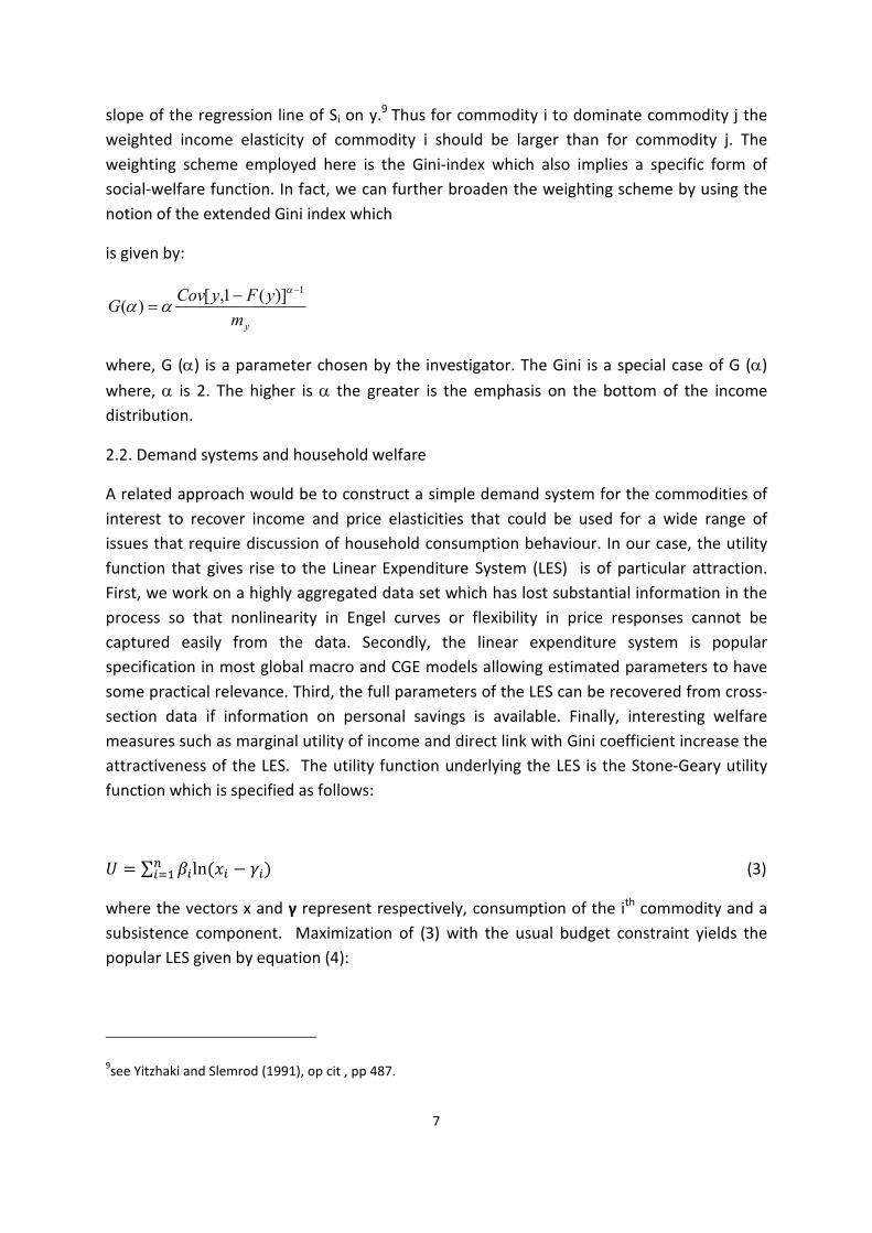
section 2, Table 3 reports parameter estimates of the Extended Linear Expenditure System
where personal savings is used to identify all the parameters. The results generally indicate
a well behaving linear relationship between demand and personal income. Our estimation
method also adjusts for possible contemporaneous correlation across equations and the
explanatory power of the linear Engel curve is also reasonably high. Generally, the marginal
budget share for some commodities is lower than the average share so that demand is
income inelastic. These are Food, Clothing, Water and Electricity, Health and Education. It is
interesting to note that household per capita expenditure on education is uniformly
distributed in all countries across Africa and the average budget share is also among the
lowest. One is tempted to relate this feature to efforts by governments to publicly provide
education services. The other interesting dimension is also the fact that average school
attainment rate vary considerably despite proportional effort by households in poor and
rich countries to invest on education. Luxury goods are the usual suspects: Alcohol,
communication, recreation, transport, restaurant related expenses, etc. Quite strikingly the
elasticity values reported for this broadly aggregated commodities is more or less consistent
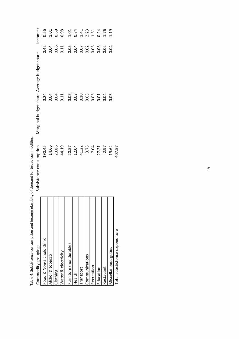
with what one often finds from large household surveys of individual countries. The price
responses indicate (Table 5) quite a dampened feature largely because of the level of
aggregation (substitution across commodities is not feasible) as well as the structure of the
ELES which is biased towards income elasticity. Another explanation is also the high value of
the Frisch parameter (or marginal utility of income) which links price elasticity with the
income elasticity. Not surprisingly, most commodities are price inelastic as reported in Table

12
(5). The main factor driving the own price elasticity in this set up is the marginal budget
share (the higher the household spends on particular commodity for a one dollar increase in
income, the larger the response to own price shocks, vice versa) and the share of
subsistence consumption in total consumption or the Frisch Parameter. The role of savings
to identify all the parameters of the ELES is crucial. Moreover, the implied marginal budget
share is also interesting. A one dollar increase in per capita income could lead to a saving of
36 cents on the average implying that savings is an income elastic “commodity” in Africa.
Finally, our estimate of total consumption expenditure needed for subsistence is close to
407 in PPP which is about 1.12 dollar a day, close to the 1.09 dollar a day conventionally
used at a global level. To a certain degree, this finding gives credence to the global poverty
line which has been under a lot of scrutiny lately (Deaton, 2009) and Deaton & xxx (2010).
5. Conclusions
This paper attempted to utilize the data generated by the ICP-Africa 2005 on 48 African
countries to extract some welfare comparisons across a broadly defined group of
commodities. No doubt that such level of aggregation may be considered a bit stretching
the underlying concept of choice theory which essentially is built on a number of restrictive
assumptions. However, the whole idea of building the ICP-Africa 2005 data is to be able to
compare standard of living across countries in a consistent framework. In that sense, then,
aggregating per capita consumption expenditure and some of its extensions such as
poverty, inequality or any other measure of welfare is allowed.
The 12 commodities covered in the ICP2005 survey are also comprehensive allowing for
some interesting inferences that may help policy dialogues. For instance, should food be
subsidized at the expense of say fuel, or should direct income transfers (such as budget
support) promote household welfare instead of some targeted expenditure say on health,
education and other necessities such as food. In dealing with these issues, certainly
household level data at a country level would be more sensible because of the realism in
policy actions. In a context where cross-country policy coordination is hardly observed our
comparison may sound “theoretical”. However there are instances where well known global
models require such inputs for their calibration. One of the most frequently used global
model if Global Trade Analysis Project which focuses on cross-regional policy simulations
such trade liberalization. One of the components modeled is household behavior where
actually the Extended Linear Expenditure System is specified to capture price and income
responses. Our computations help identify these parameters for such exercises easily.
Often, available country information is imputed for the whole region to run the models.
Thus, our results may fill these gaps.
The other interesting dimension of this global demand analysis is that the estimated
parameters strikingly are close to what one would obtain from household surveys in this

13
settings. There is nothing strange or out of the ordinary in our estimates of income and price
elasticity values. Finally, even our poverty line estimate from “subsistence” expenditure
implied by the model is very close to the international poverty line which was computed
using a completely different approach.

14
References
Ahmad ,E., and Stern, N., (1984), The Theory Of Indirect Tax Reform and Indian Indirect
Taxes, Journal Of Public Economics, 25, 259-298.
Atkinson, A.B., 1970, “The Measurement of Inequality, Journal of Economic Theory, 2, 244-263.
Ahmad, S. (2006), “Historical overview of International Comparison Program”, mimeo World
Bank
Chen, Shaohua & Ravallion, Martin, 2008. "The developing world is poorer than we thought,
but no less successful in the fight against poverty," Policy Research Working Paper Series
4703, The World Bank.
Chen, Shaohua & Ravallion, Martin, 2007. "The changing profile of poverty in the world:,"
2020 vision briefs BB01 Special Edition, International Food Policy Research Institute (IFPRI).
Chen, Shaohua & Ravallion, Martin, 2007. "Absolute poverty measures for the developing
world, 1981-2004," Policy Research Working Paper Series 4211, The World Bank
Chen, Shaohua & Ravallion, Martin, 2004. "How Have the World's Poorest Fared Since the
Early 1980s?," Policy Research Working Paper Series 3341, The World Bank:
Cragg, M., 1991, Do we care; A study of Canada's Indirect Tax System’ Canadian Journal of
Economics, XXIV, No.1. Feb, 124-143
Davidson. R., Duclos, J.Y. 2000. "Statistical Inference for Stochastic Dominance and for the
Measurement of Poverty and Inequality,"Econometrica, Vol. 68 (6) pp. 1435-1464.
Deaton, A.S. (2009) “Purchasing Power Parity Exchange Rates for the Global Poor”, memo,
Princeton University
Deaton, A.S., 1981, Optimal Taxes and The Structure of Preferences, Econometrica, Vol.49,
1245-1260
Deaton, A. and J. Mullbeauer (1980): Economics and Consumer Behaviour, Cambridge
University Press. Cambridge
Dowrick, Steve (2005). Errors in the Penn World Table demographic data. Economics Letters,
86, 243-248.

15
Dowrick, Steve and Quiggin, John (1997). True measures of GDP and convergence. American
Economic Review, 87, March, 41-64.
Ferreira, Francisco H.G. & Ravallion, Martin, 2008. "Global poverty and inequality : a review
of the evidence," Policy Research Working Paper Series 4623, The World Bank
Hagenaars, A., 1987, A Class of Poverty Indices, International Economic Review, vol 28, no. 3,
583-607.
Haggablade, S and Younger. S. 2003. Indirect Tax Incidence in Madagascar: Updated
Estimates Using the Input-Output Table. Mimeo.
Heston, Alan and Summers, Robert (1996). International price and quantity comparisons:
potentials and pitfalls. American Economic Review, 86(2), May.
Kakwani, N., 1980 Income Inequality, and Poverty: Methods of Estimation and Policy
Applications, Oxford University Press
King., M., 1983, Welfare Analysis of Tax Reform, Journal of Public Economics, 21, 183-241
Knowles, Stephen (2001) Are the Penn World Tables data on government consumption and
investment being misused? Economics Letters, May, 71(2), 293-98.
Kravis, Irving B. (1984) Comparative studies of national income and prices. Journal of
Economic Literature, 22, March, 1-39.
Marris, Robin (1984) Comparing the incomes of nations: a critique of the international
comparison project. Journal of Economic Literature, 22, 40-57.
Nuxoll, Daniel A. (1994) Differences in relative prices and international differences in growth
rates. American Economic Review, 84, December, 1423-36.
Summers, Robert and Heston, Alan (1988). A new set of international comparisons of real
product and price levels estimates for 130 countries, 1950-1985, Review of Income and
Wealth, 34(1), March, 1-25.
Summers, Robert and Heston, Alan (1991). The Penn World Table (Mark 5): an expanded set
of international comparisons, 1950-1988, Quarterly Journal of Economics, 106(2), May, 327-
68.
Thomas W. Hertel and Marinos E. Tsigas (1997)” Structure of GTAP” in in T.W. Hertel (ed.),
Global Trade Analysis: Modeling and Applications, Cambridge University Press

16
Table 1: African countries covered under ICP2005
Country Per capita consumption expenditure in PPP
Angola 310.1237
Benin 485.8138
Botswana 1334.234
Burkina Faso 376.5132
Cameroon 672.3389
Cape Verde 1153.902
Central African Republic 309.1735
Chad 363.1584
Comoros 414.3654
Congo 364.2758
Congo, Democratic Republic 68.19534
Côte d'Ivoire 525.9131
Djibouti 519.0859
Egypt 1653.074
Equatorial Guinea 1309.882
Ethiopia 216.5842
Gabon 1253.719
Gambia 190.3816
Ghana 436.3439
Guinea 291.603
Guinea-Bissau 196.8927
Kenya 553.1107
Lesotho 774.3787
Liberia 117.9258
Madagascar 342.5094
Malawi 235.8604
Mali 337.821
Mauritania 518.0571
Mauritius 3383.374

17
Morocco 1125.192
Mozambique 265.0105
Namibia 1257.736
Niger 215.5689
Nigeria 561.6708
Rwanda 270.6373
Sao Tome and Principe 658.5045
Senegal 610.9812
Sierra Leone 317.7314
South Africa 2607.232
Sudan 857.7122
Swaziland 1412.419
Tanzania 370.8047
Togo 414.1749
Tunisia 2066.349
Uganda 332.0936
Zambia 356.9883
Zimbabwe 179.5134
Mean 699.5871
Table 2: summary statistics
Average expenditure ratios Obs Mean Std. Dev. Min Max
Food expenditure 47 0.417 0.172 0.124 1.005
Saving ratio 47 0.138 0.202 -0.512 0.649
Water 47 0.111 0.039 0.035 0.253
Transport services 47 0.072 0.042 0.012 0.190
Clothing 47 0.059 0.040 0.012 0.254
Household utensils 47 0.050 0.021 0.004 0.131
Miscellaneous goods 47 0.041 0.024 0.000 0.118
Health 47 0.040 0.038 0.004 0.197
Alcohol & tobacco 47 0.036 0.035 0.001 0.196
Education 42 0.031 0.038 0.002 0.200
Recreation 47 0.027 0.021 0.004 0.114
Restaurant 47 0.023 0.027 0.000 0.145
Communication 47 0.016 0.016 0.001 0.070

18
Table 3: Seemingly Unrelated Regression estimate for the ELES parameters: Dependent variable is disposable
income
Broad consumption categories Coefficient SD Z-value
Food and Non-alcohol 0.2354997 0.0149967 15.7
_cons 94.46787 18.56974 5.09
Alcohol 0.0359582 0.0044822 8.02
_cons -1.329985 5.550114 -0.24
Clothing 0.0411219 0.0032226 12.76
_cons 7.096983 3.990449 1.78
Water and electricity 0.1084259 0.006779 15.99
_cons -5.494426 8.39417 -0.65
Household utensils 0.0504609 0.0032221 15.66
_cons -0.508313 3.989752 -0.13
Health 0.0295296 0.0049542 5.96
_cons 6.657909 6.13454 1.09
Transport 0.101146 0.0080871 12.51
_cons -13.8858 10.01395 -1.39
Communications 0.034621 0.0032386 10.69
_cons -10.35782 4.010236 -2.58
Recreation 0.0349589 0.0028717 12.17
_cons -7.204188 3.555852 -2.03
Education 0.0072792 0.0029862 2.44
_cons 10.93661 3.697714 2.96
Restaurant 0.0399303 0.0084184 4.74
_cons -8.301922 10.42416 -0.8
Miscellaneous goods 0.048131 0.0039291 12.25
_cons -3.145296 4.865252 -0.65
Breusch-Pagan test of independence: chi2(66) = 224.531, Pr = 0.0000
19
Ta
ble
4:
Su
bsi
ste
nce
co
nsu
mp
tio
n a
nd
in
com
e e
last
icit
y o
f d
em
an
d f
or
bro
ad
co
mm
od
itie
s
Co
mm
od
ity
gro
up
ing
sS
ub
sist
en
ce c
on
sum
pti
on
Ma
rgin
al
bu
dg
et
sha
reA
ve
rag
e b
ud
ge
t sh
are
Inco
me
ela
stic
ity
Fo
od
& N
on
-alc
ho
ld d
rin
k1
90
.45
0.2
40
.42
0.5
6
Alc
ho
l &
to
ba
cco
14
.66
0.0
40
.04
1.0
1
Clo
thin
g2
3.8
60
.04
0.0
60
.69
Wa
ter
& e
lect
rici
ty4
4.1
90
.11
0.1
10
.98
Fu
rnit
ure
(n
on
du
rab
le)
20
.57
0.0
50
.05
1.0
1
He
alt
h1
2.0
40
.03
0.0
40
.74
Tra
nsp
ort
41
.22
0.1
00
.07
1.4
1
Co
mm
un
ica
tio
ns
3.7
50
.03
0.0
22
.23
Re
cre
ati
on
7.0
40
.03
0.0
31
.31
Ed
uca
tio
n2
7.2
10
.01
0.0
30
.24
Re
sta
ua
nt
2.9
70
.04
0.0
21
.76
Mis
cell
an
eo
us
go
od
s1
9.6
20
.05
0.0
41
.19
To
tal
sub
stis
ten
ce e
xpe
nd
itu
re4
07
.57

20
Ta
ble
5:
cro
ss a
nd
ow
n p
rice
ela
stic
ity
va
lue
s fr
om
th
e E
LES
F
oo
d &
No
n-
alc
ho
ld d
rin
k
Alc
ho
l &
tob
acc
o
Clo
thin
g
Wa
ter
Fu
rnit
ure
(no
nd
ura
ble
) H
ea
lth
T
ran
spo
rt
Co
mm
un
ica
tio
ns
Re
cre
ati
on
E
du
cati
on
R
est
au
an
t
Mis
cella
ne
ou
s
go
od
s
Fo
od
& N
on
-alc
ho
ld d
rin
k
-0.4
86
-0
.12
5
-0.1
38
-
0.1
22
-0
.11
8
-
0.0
94
-0
.14
1
-0.0
49
-0
.07
3
-0.1
90
-0
.02
9
-0.1
28
Alc
ho
l & t
ob
acc
o
-0.1
77
-0
.48
9
-0.0
21
-
0.0
19
-0
.01
8
-
0.0
14
-0
.02
2
-0.0
07
-0
.01
1
-0.0
29
-0
.00
4
-0.0
20
Clo
thin
g
-0.1
21
-0
.01
3
-0.4
37
-
0.0
41
-0
.01
9
-
0.0
14
-0
.02
5
0.0
01
-0
.01
0
-0.0
04
-0
.00
5
-0.0
15
Wa
ter
& e
lect
rici
ty
-0.1
71
-0
.01
9
-0.0
28
-
0.5
38
-0
.02
7
-
0.0
19
-0
.03
5
0.0
01
-0
.01
4
-0.0
06
-0
.00
8
-0.0
22
Fu
rnit
ure
(n
on
du
rab
le)
-0.1
76
-0
.01
9
-0.0
28
-
0.0
60
-0
.52
3
-
0.0
20
-0
.03
6
0.0
01
-0
.01
4
-0.0
07
-0
.00
8
-0.0
22
He
alt
h
-0.1
29
-0
.01
4
-0.0
21
-
0.0
44
-0
.02
0
-
0.6
14
-0
.02
6
0.0
01
-0
.01
0
-0.0
05
-0
.00
6
-0.0
16
Tra
nsp
ort
-0
.24
7
-0.0
27
-0
.04
0
-
0.0
84
-0
.03
8
-
0.0
28
-0
.46
1
0.0
01
-0
.02
0
-0.0
09
-0
.01
1
-0.0
31
Co
mm
un
ica
tio
ns
-0.3
89
-0
.04
3
-0.0
63
-
0.1
33
-0
.06
1
-
0.0
44
-0
.07
9
-0.8
00
-0
.03
1
-0.0
14
-0
.01
7
-0.0
49
Re
cre
ati
on
-0
.22
9
-0.0
25
-0
.03
7
-
0.0
78
-0
.03
6
-
0.0
26
-0
.04
7
0.0
01
-0
.70
0
-0.0
09
-0
.01
0
-0.0
29
Ed
uca
tio
n
-0.0
42
-0
.00
5
-0.0
07
-
0.0
14
-0
.00
6
-
0.0
05
-0
.00
8
0.0
00
-0
.00
3
-0.1
97
-0
.00
2
-0.0
05
Re
sta
ua
nt
-0
.30
6
-0.0
34
-0
.04
9
-
0.1
05
-0
.04
8
-
0.0
34
-0
.06
3
0.0
01
-0
.02
5
-0.0
11
-0
.87
8
-0.0
39
Mis
cella
ne
ou
s g
oo
ds
-0.2
07
-0
.02
3
-0.0
33
-
0.0
71
-0
.03
2
-
0.0
23
-0
.04
2
0.0
01
-0
.01
7
-0.0
08
-0
.00
9
-0.4
81
75

21
Figure 1: Share of food in total consumption expenditure in Africa: 2005
Figure 2: Engel function for Food expenditure
.25
.3.35
.4.45
Share of food in total expenditure
0 1000 2000 3000 4000Per capita consumption expenditure
01000
2000
3000
4000
Food & drinks; disposable income
0 1000 2000 3000 4000disposable income
Food Engel curve 45 degree line

22
Figure 3: Concentration curve for selected commodities in Africa using data from ICP 2005
Figure 4: Concentration curve for selected commodities in Africa using data from ICP 2005
0.2
.4.6
.81
L(p)
0 .2 .4 .6 .8 1Percentiles (p)
line_45° Food per capita expenditure
Per capita exp on transport Total per capita expenditure
Per capita disposable income
0.2
.4.6
.81
C(p)
0 .2 .4 .6 .8 1Percentiles (p)
line_45° Food per capita expenditure
Per capita health expenditure Per capita expenditure on education
Per capita disposable income