lable at ScienceDirect

Atmospheric Environment 44 (2010) 4426e4431

Contents lists avai

Atmospheric Environment

journal homepage: www.elsevier .com/locate/atmosenv

An adaptive reduction algorithm for efficient chemical calculations in globalatmospheric chemistry models

Mauricio Santillana a,*, Philippe Le Sager b,1, Daniel J. Jacob b, Michael P. Brenner b

aHarvard University Center for the Environment, Cambridge, MA 02138, United Statesb School of Engineering and Applied Sciences, Harvard University, Cambridge, MA 02138, United States

a r t i c l e i n f o

Article history:Received 13 April 2010Received in revised form16 July 2010Accepted 21 July 2010

Keywords:Atmospheric chemistryMulti-scale analysisTime-scale separationReduction of chemical kinetics

* Corresponding author. Tel.: þ1 617 495 5941.E-mail address: msantill@fas.harvard.edu (M. Sant

1 Now at Royal Netherlands Meteorological Institut

1352-2310/$ e see front matter � 2010 Elsevier Ltd.doi:10.1016/j.atmosenv.2010.07.044

a b s t r a c t

We present a computationally efficient adaptive method for calculating the time evolution of theconcentrations of chemical species in global 3-D models of atmospheric chemistry. Our strategy consistsof partitioning the computational domain into fast and slow regions for each chemical species at everytime step. In each grid box, we group the fast species and solve for their concentration in a coupledfashion. Concentrations of the slow species are calculated using a simple semi-implicit formula. Sepa-ration of species between fast and slow is done on the fly based on their local production and loss rates.This allows for example to exclude short-lived volatile organic compounds (VOCs) and their oxidationproducts from chemical calculations in the remote troposphere where their concentrations are negli-gible, letting the simulation determine the exclusion domain and allowing species to drop out individ-ually from the coupled chemical calculation as their production/loss rates decline. We applied ourmethod to a 1-year simulation of global tropospheric ozone-NOx-VOC-aerosol chemistry using the GEOS-Chem model. Results show a 50% improvement in computational performance for the chemical solver,with no significant added error.

� 2010 Elsevier Ltd. All rights reserved.

1. Introduction

Understanding the global-scale dynamics of the chemicalcomposition of our atmosphere is essential for addressing a widerange of environmental issues from air quality to climate change.Global 3-D models of tropospheric chemistry must solve a systemof coupled non-linear advection-reaction partial differential equa-tions representing the temporal evolution of the different reactivespecies. Typical chemical mechanisms include over 100 specieswith lifetimes ranging from milliseconds to many years, giving riseto very large and stiff systems of differential equations. Solvingthese equations is difficult and the development of efficient andaccurate techniques to achieve this has inspired research for thepast 40 years. See for example (Jacobson,1999; Sportisse, 2007) andthe multiple references therein. A particular challenge for globalmodels is to describe the full range of chemical environmentsincluding concentrated source regions that may have a large global

illana).e.

All rights reserved.

influence. We show here that it is possible to achieve substantialcomputational savings by an adaptive method that dynamicallyadjusts the chemical mechanism to be solved to the local envi-ronment. We demonstrate the accuracy and performance of themethod by application to the GEOS-Chem global chemical trans-port model (Bey et al., 2001).

Tropospheric chemistry models simulate the chemical compo-sition of the atmosphere using a set of coupled non-linear partialdifferential equations of the type:

vCivt

þ u$VCi ¼ Pi � Li; i ¼ 1;.;N (1)

where Ci (x,t) represents the spatio-temporal evolution of theconcentration of species i, u(x,t) is the wind velocity,Pi ¼ PiðfCjg; x; tÞ is the ensemble of atmospheric sources, and Li ¼LiðfCjg; x; tÞ is the ensemble of atmospheric sinks. The speciescoupling shows up locally in Pi and Li, through the group ofchemical species {Cj} that produce or react with species i. Pi and Liare also functions of the local radiative and meteorological envi-ronment. The number of species N is typically over 100.

Equations (1) are solved in 3-D models using operator splittingmethods that integrate the advection and chemistry operators

M. Santillana et al. / Atmospheric Environment 44 (2010) 4426e4431 4427

separately. This enormously reduces the degrees of freedom of thenon-linear system (Hundsdorfer and Verwer, 2003). In a simulationincluding detailed oxidant chemistry, the solution of the stiffsystem of ordinary differential equations (ODE):

dCidt

¼ Pi��

Cj��� Li

��Cj��

; i ¼ 1;.;N; (2)

is the most time consuming process in the chemistry operatorintegration. Approaches to speed up this process include fastcomputational algorithms (Jacobson and Turco, 1994), and efficientnumerical schemes such as implicit Rosenbrock solvers (Sanduet al., 1997; Damian et al., 2002). Other or complementary strate-gies use asymptotic analysis arguments, parameterization tech-niques, species lumping, or simplifications of chemical processes inparticular locations of the domain. Examples include the separationof fast and slow species (Young and Boris, 1977; Gong and Cho,1993), the quasi-steady-state assumption (QSSA) methods(Hesstvedt et al., 1978), functional parameterization of box modelresults (Jacob et al., 1989), species lumping (Sportisse and Djouad,2000), and the use of different mechanisms for different regionseither with specified boundaries (Jacobson, 1995) or with locallydetermined boundaries (Rastigeyev et al., 2007). Most approachesbased on asymptotic analysis or parameterizations have beenoptimized for a given type of chemical regime and do not have theflexibility for implementation in a global model with a very widerange of possible regimes.

Separation of chemical mechanisms by geographical domains isparticularly attractive for global models. Much of the complexity inthese models is driven by short-lived non-methane volatile organiccompounds (NMVOCs) emitted at the surface, which oxidize toa cascade of decomposition products of varying lifetimes. TheseNMVOCs and their short-lived decomposition products can beneglected inmost of the troposphere, and their location-dependentexclusion from the chemical mechanism can greatly speed up thechemical computation. A challenge is to formulate this exclusionproperly. Pre-setting geographical boundaries (as in Jacobson,1995) is problematic because of the continuum of atmosphericlifetimes in NMVOCs and their oxidation products, and because offast processes (such as deep convection) that can occasionally causeshort-lived species to influence the remote troposphere far fromtheir point of emission. Rastigeyev et al. (2007) presented analgorithm to locally diagnose a “chemical boundary layer” forindividual species outside of which the species would be excludedfrom the mechanism and its concentration extrapolated by expo-nential decay. But this was only implemented in idealized scenariosof simple flow and chemistry.

In this work, we propose an algorithm that partitions, locallyand on the fly, the global domain into fast and slow regions for eachspecies, and adapts the solution strategy to the local environmentdynamically in space and time. In this way our algorithm is adap-tive. The proposed algorithm is implemented and tested usingrealistic meteorological conditions and full ozone-NOx-VOC-aerosolchemistry.

2. The algorithm

Let us first re-write the chemistry operator as

dCidt

¼ Pi � kiCi; i ¼ 1;.;N (3)

since generally (though not always) the loss terms Li have first-order dependence on the species concentration Ci. Here ki is aneffective loss rate constant. Asymptotic analysis arguments such asthose utilized in low-dimensional manifold reduction methods

(Lowe and Tomlin, 2000; Kaper and Kaper, 2002) and reducedchemical models (Djouad and Sportisse, 2003) show that one canseparate species, based on the relative magnitude of the right-handside of (3), as fast if dCi/dt > d or slow if dCi/dt � d, for a smallparameter d, and compute an approximate solution to the ODEsystem (3) by only solving for the the group of fast species asa coupled system, and solving for the slow species either as analgebraic system (dCi/dt z 0) or using a low-order numericalscheme (dCi/dt z d). By construction, this family of approximatesolutions for different values of d converges to the solution of thesystem (3) provided d/0. Following these ideas, in our algorithm,at every grid box and time step tn, we identify as fast species thosesatisfying either Piðx; tnÞ > d or Liðx; tnÞ > d, and calculate theirconcentrations {Cinþ1 ¼ Ci (tnþ1)} at the next time step,tnþ1 ¼ tn þ Dt, in a coupled fashion using an efficient implicit ODEsolver for stiff systems, such as Gear-type or Rosenbrock. Theconcentrations of the rest of the (slow) species will not changemuch over a given time step since dCi/dt z 0 or at most dCi/dt z d,suggesting that we can treat Pi¼ Pi* and ki¼ ki* as constant for t˛ [tn,tn þ Dt] (Young and Boris, 1977; Hesstvedt et al., 1978) andanalytically solve Eq. (3) to obtain the formula

Cnþ1i ¼ P*i

k*iþ Cni � P*i

k*i

!e�k�i Dt (4)

to calculate their evolution separately.The choice of an appropriate small parameter or threshold d can

be guided by simple reasoning. The general problem of tropo-spheric oxidant chemistry is in large part driven by reactions of theOH radical and ensuing radical chains. OH has a daytime concen-trationw106molecules cm�3 and a lifetimew1 s. It follows that thechemical production and loss rates for important species in the fastmechanism (i.e., the Pi and kiCi terms) may be expected to bewithina few orders of magnitude of 106 molecules cm�3 s�1. A species forwhich both production and loss rates are less than 102 moleculescm�3 s�1, is unlikely to play a significant role in coupling to otherspecies in the fast mechanism. This does not necessarily mean thatthe species is atmospherically unimportant, only that it is notsignificantly coupled to the other species.

Even though non-conservation of mass can arise from solvingfast and slow species using different expressions, these massimbalances can be controlled by choosing an adequate thresholdd based on the production and loss rates. Indeed, in Sect. 4.2, wefind that a long-duration simulation (1 year) using our adaptivealgorithm for d < 102 molecules cm�3 s�1 compares successfullywith a benchmark simulation, making the issue of mass conser-vation negligible.

3. Implementation

We implemented our algorithm using the GEOS-Chem model(version v8-02-02). GEOS-Chem is a state-of-the-art 3-D globalmodel of tropospheric chemistry driven by assimilated meteoro-logical observations from the Goddard Earth Observing System(GEOS) of the NASA Global Modeling and Assimilation Office(GMAO). Themodel simulates global tropospheric ozone-NOx-VOC-aerosol chemistry. The full chemical mechanism for the tropo-sphere involves 111 species and over 300 reactions.

The chemical mass balance equations are integrated usinga Gear-type solver (SMVGEAR II, Jacobson (1995)). Stratosphericchemistry is not explicitly simulated and it is instead parameterizedto provide a proper representation of cross-tropopause fluxes. Weused GEOS-Chemwith a 4

� � 5�horizontal resolution and 20 sigma

levels in the vertical for the following examples. For a detaileddescription of the original model see (Bey et al., 2001).

M. Santillana et al. / Atmospheric Environment 44 (2010) 4426e44314428

We performed three sets of simulations. The first two consistedof one-week long simulations aimed at selecting an appropriatethreshold d, and initialized on July 1st, 2004. The third one consistedof one-year simulations for 2005 aimed at testing the algorithm forthe range of relevant time-scales of the system. The initial conditionfor the latter was obtained by running the model during 6 monthsprior to Jan 1st, 2005 (From Jul 1st, 2004 to Jan 1st, 2005) using thedefault settings (including the standard solver: SMVGEAR II).

We implemented our algorithm using LSODES (LivermoreSolver for Ordinary Differential Equations; Radhakrishnan andHindmarsh (1993)) instead of SMVGEAR II because it could bemore easily configured to solve a different non-linear ODE systemat each grid box at each time step. Wewill elaborate on this issue inSect. 4.

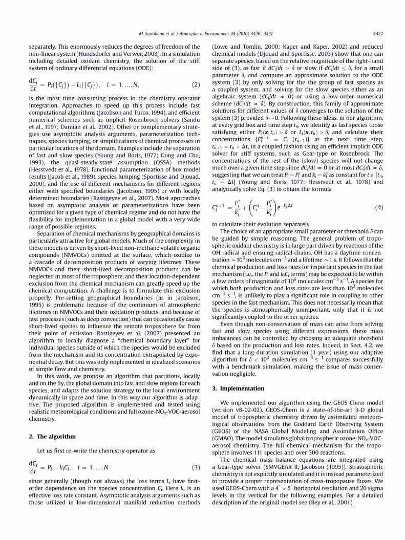
Fig. 1 illustrates the partitioning between fast and slow speciesfor peroxyacetylnitrate (PAN) and isoprene for a threshold ofd ¼ 102 molecules cm�3 s�1 and for July 8, 2004 at 0 GMT. Isopreneis emitted by vegetation and has a chemical lifetime ofw1 h againstoxidation by OH. In continental boundary layers where isopreneemissions are important, one needs to track isoprene and itssuccessive oxidation products (about 40 species in the GEOS-Chemmechanism; Horowitz et al. (1998)) as part of the ensemble of fastspecies. Outside of the continental boundary layer, however,isoprene concentrations drop to negligibly low levels and can thenbe excluded from solution in the fast mechanism (note localizedexceptions over Brazil and Southeast Asia where deep convectioninjects isoprene to the upper troposphere). As air parcels furtherage, the isoprene oxidation products gradually drop out from thefast mechanism. In this manner, the fast mechanism is considerablysimplified in the free troposphere or over the oceans to excludemost isoprene chemistry.

The right panels of Fig. 1 show the fast-slow boundary for PAN.PAN is a particularly complicated molecule in a scale-separationscheme. It is produced by photochemical oxidation of NMVOCs inthe presence of NOx, most vigorously in the continental boundary

Fig. 1. Partitioning between fast and slow regions for isoprene and PAN (0.3 and 10 km abovon July 8, 2004 at 00 GMT.

layer but also at a slower rate in the global troposphere from thelong-lived VOCs ethane and acetone. Its lifetime against thermaldecomposition is less than 1 h at room temperature but increases toseveral months in the upper troposphere. Its long lifetime at coldtemperatures allows it to be transported on a global scale toeventually release NOx thermally or photochemically in the remotetroposphere. We see from Fig. 1 that PAN needs to be included inthe fast mechanism everywhere except in places that are very coldand dark (note the boundary between fast/slow regions at theterminator line in the upper troposphere) or warm and very remote(Indian Ocean near the surface).

Fig. 2 shows the percentage of the 111 species in the GEOS-Chemchemical mechanism that are treated as fast, for a threshold d¼ 102

molecules cm�3 s�1. The percentage of fast species globally is 39%.There is no grid box in the domainwhere all the 111 species are fast.This is because some species are fast only in the daytime whileothers are fast only at night. Fig. 3 shows, for selected species, thepercentage of tropospheric grid boxes where they are fast. Short-lived hydrocarbons are fast in only a small fraction of the grid boxes.OH, ozone, and NO2 are fast almost everywhere.

4. Testing the algorithm

We evaluated our adaptive algorithm by comparison witha benchmark LSODES simulation including all species treated asfast. We chose the Relative Root Mean Square (RRMS) metric asgiven by in Sandu et al. (1997)

dABðCiÞ ¼ffiffiffiffiffiffiffiffiffiffiffiffiffiffiffiffiffiffiffiffiffiffiffiffiffiffiffiffiffiffiffiffiffi1M

XU

�����CAi � CB

i

CAi

�����vuut

2

(5)

where CiA and Ci

B are the concentrations of species i calculated insimulations A and B, respectively,U is the set of grid boxes where CiA

e surface) using as threshold d ¼ 102 molecules cm�3 s�1. Results are from GEOS-Chem

Fig. 2. Percentage of fast species in the GEOS-Chem chemical mechanism at different altitudes using a threshold of d ¼ 102 molecules cm�3 s�1. White boxes in the bottom rightpanel are in the stratosphere. Results are for July 8, 2004 at 00 GMT. The full GEOS-Chem chemical mechanism includes 111 species to describe tropospheric ozone-NOx-VOC-aerosol chemistry.

M. Santillana et al. / Atmospheric Environment 44 (2010) 4426e4431 4429

exceeds a threshold a, and M is the number of such grid boxes. Weused a¼ 106molecules cm�3 as in Eller et al. (2009) for our analysis.

4.1. Selection of threshold rate for fast mechanism

We performed two sets of 5 one-week GEOS-Chem ozone-NOx-VOC-aerosol chemistry simulations using the values d ¼ 0 (all

Fig. 3. Percentage of tropospheric grid boxes where particular species are fast usinga threshold rate of d ¼ 102 molecules cm�3 s�1. Results are from a GEOS-Chemsimulation on July 8, 2004 at 00 GMT.

species are fast), 10, 102, 103, 104 molecules cm�3 s�1. The first set ofsimulations were carried out in a chemistry-only mode (no trans-port) in order to assess the accuracy of our algorithm without thepresence of any other mechanism. The second set was performed ina realistic configuration with all mechanisms of the code turned“on”, we refer to this set as chemistry and transport simulations. Inthese numerical experiments, we compared the daily-averagedconcentrations of species in the last day of the simulations usingour adaptive algorithm for a given d > 0, with a benchmark simu-lation solving for all species as fast (standard method in GEOS-Chem).

The results of the experiments, presented in Fig. 4, show for eachthreshold d an average value of the percentage of fast speciesduring the simulation (top). The red data points show that thecomputational cost of the solver decreases linearly with thedecrease of percentage of species, n, solved with the fast mecha-nism (100% corresponds to the CPU time used by the solver ina simulation with all species solved as fast, d ¼ 0). This is a conse-quence of the OðnÞ efficiency of the sparse linear algebra routinesused by LSODES. The blue and green data points show the medianRRMS of the difference over all species between the benchmarksimulation LSODES (all species fast) and the adaptive algorithmsimulations for the different thresholds, in chemistry-only andchemistry and transport modes, respectively. Note that the RRMS ofthe differences of the chemistry and transport simulations arereduced when compared to the ones in chemistry-only mode. Thismay reflect the compensation of errors by transport, but also themaintenance of concentrations in a more realistic range over the 1-week simulation. In both modes, RRMS differences are negligible(<1%) when using a threshold d ¼ 10 molecules cm�3 s�1 withsignificant savings of about 40%. For d¼ 102molecules cm�3 s�1, themedian RRMS is less than 3% in the chemistry and transport

Fig. 4. Accuracy and performance of the adaptive reduction algorithm as a function ofthe production/loss rate threshold d used to separate fast and slow species. The blueand green curves show the median RRMS over all species in chemistry-only andchemistry and transport modes respectively, the red curve shows the percentage of thecomputer time used for the chemical solver relative to a full-chemistry calculation(d ¼ 0). The top scale shows the global percentage of species solved as fast for thedifferent values of delta. Results are for 1-week simulations initialized on July 1, 2004.(For the interpretation of the reference to color in this figure legend the reader isreferred to the web version of this article.)

M. Santillana et al. / Atmospheric Environment 44 (2010) 4426e44314430

simulations, while the computational time utilized by the solver iscut in half and the percentage of species being solved as fast is 39%.Using a higher threshold d ¼ 103 molecules cm�3 s�1 incursa significantly larger RRMS for only a 12% gain in the chemicalsolver computational requirement as compared to using d ¼ 102

Fig. 5. Time evolution of the RRMS for four selected species (NOx, CO, OH, and O3) for one-yea simulation using our algorithm with d ¼ 102 molecules cm�3 s�1 to a reference simulatioSMVGEAR II solvers with all species fast.

molecules cm�3 s�1. Since the purpose of our algorithm is toprovide an accurate solution in realistic simulations with couplingbetween chemistry and transport, we conclude that d ¼ 102

molecules cm�3 s�1 is optimal.

4.2. One-year comparison

Based on the results of the previous section, a more compre-hensive test of the accuracy of our algorithm was carried out fora one-year GEOS-Chem simulation of ozone-NOx-VOC-aerosolchemistry. This approach allows the sampling of the range ofexpected conditions and also tests the longer-lived species. Weconducted three different one-year long simulations: the first oneusing our adaptive algorithm with a threshold value of d ¼ 102

molecules cm�3 s�1, the second one using LSODES with all speciessolved as fast, and the third one using GEOS-Chem’s standardchemistry solver SMVGEAR II. All three simulations were identicalexcept for the chemistry solver.

Fig. 5 shows the time evolution of the RRMS of differencesbetween our algorithm and the standard (LSODES solver) simula-tions, for four selected species: NOx, CO, OH, and O3. Also shown isthe comparison between the LSODES solver (all species fast) andSMVGEAR II. Note that the relative differences between our algo-rithm and the reference simulation do not exceed 5% for NOx andare below 1% for CO, OH, and O3. These differences are of the samemagnitude as those observed between LSODES and SMVGEAR IIwith full-chemistry. We conclude that our adaptive algorithm doesnot induce significant errors relative to the full solution.

5. Conclusions

We presented a computationally efficient adaptive algorithm tocalculate the time evolution of the concentrations of chemicalspecies in global 3-D models of atmospheric chemistry.

Our algorithm identifies on the fly where a particular species isimportant (fast) or unimportant (slow) in the coupled chemicalmechanism by comparing its production and loss rates witha prescribed threshold d, and then adjusts the solution strategyaccordingly. We solve for the concentration of fast species using thestandard implicit solver of the model, and use an efficient semi-implicit formula for the slow species. The choice of the thresholdd is motivated by the observation that the characteristic magnitudeof the production or loss rates driving the evolution of the coupledsystem are of the order of 106 molecules cm�3 s�1. Thus, a speciesfor which both production and loss rates are < 102 moleculescm�3 s�1 does not significantly drive the coupling of the system.

ar (2005) simulations. Daily average at the end of each month. The left panel comparesn (LSODES d ¼ 0, all species fast). The right panel compares the standard LSODES and

M. Santillana et al. / Atmospheric Environment 44 (2010) 4426e4431 4431

A central advantage of our method for global 3-D model appli-cations is to resolve the large differences in the complexity of therelevant mechanism between different regions of the world. Forexample, short-lived NMVOCs and their decomposition productsmay be important contributors to the chemical mechanism incontinental boundary layers but not in the rest of the world. Bydiagnosing the relevant mechanism for a particular grid box on thefly, our method avoids the problematic prejudgment of wherea species may be important.

We present a comprehensive evaluation of our algorithm inSect. 4.1 with a 7-day ozone-NOx-VOC-aerosol chemistry simula-tion using different thresholds d in the GEOS-Chem global 3-Dmodel in a chemistry-only mode (transport turned off) and in theactual model with coupling between chemistry and transport.Coupling between chemistry and transport alleviates errors, whichmay reflect both error compensation during transport but also themaintenance of concentrations in more realistic ranges. In bothcases, a threshold of d ¼ 10 molecules cm�3 s�1 reduces the timeintegration of the chemistry solver by 40%, solving approximately50% of species as fast, while showing negligible differences (<1%)when compared to a reference simulation. A larger threshold valueof d ¼ 102 molecules cm�3 s�1 still incurs errors of less than 3% inthe coupled chemistry-transport simulation while cutting the timeintegration of the chemistry solver in half by solving approximately40% of species as fast.

We show that the differences between a 1-year benchmarksimulation, and a 1-year simulation using our algorithm do not growintime, and infactareof similarmagnitudeasdifferencesbetweenthetwo well-established solvers SMVGEAR and LSODES. These differ-ences are less than 5% for NOx and are below 1% for CO, OH, and O3during the year. This finding validates the efficiency of our approachfor a broad range of time-scales and shows that issues of massconservation are negligible for the choice d¼ 102molecules cm�3 s�1.

Acknowledgements

MS thanks the Harvard University Center for the Environmentfor the Henson Environmental Fellowship that funded his contri-bution for this investigation. PLS and DJJ were supported by theNASA Atmospheric Composition Modeling and Analysis Program.MPB was supported by the NSF Division of Mathematical Sciences.The authors thank Claire Carouge and Richard Ramaroson forvaluable discussions. The authors thank the valuable commentsand suggestions made by two anonymous reviewers.

References

Bey, I., Jacob, D.J., Yantosca, R.M., Logan, J.A., Field, B., Fiore, A.M., Li, Q., Liu, H.,Mickley, L.J., Schultz, M., 2001. Global modeling of tropospheric chemistry withassimilated meteorology: model description and evaluation. Journal ofGeophysical Research 106, 23,073e23,096.

Damian, V., Sandu, A., Damian, M., Potra, F., Carmichael, G.R., 2002. The kineticpreprocessor KPP-a software environment for solving chemical kinetics.Computers & Chemical Engineering 26 (11), 1567e1579.

Djouad, R., Sportisse, B., 2003. Solving reduced chemical models in air pollutionmodelling. Applied Numerical Mathematics 44 (1e2), 49e61.

Eller, P., Singh, K., Sandu, A., Bowman, K., Henze, D.K., Lee, M., 2009. Implementationand evaluation of an array of chemical solvers in the global chemical transportmodel GEOS-Chem. Geoscientific Model Development 2, 89e96.

Gong, W., Cho, H.R., 1993. A numerical scheme for the integration of the gas-phasechemical rate equations in three-dimensional atmospheric models. Atmo-spheric Environment 27A, 2147e2160.

Hesstvedt, E., Hov, O., Isaksen, I., 1978. Quasi-steady-state-approximation in airpollution modelling: comparison of two numerical schemes for oxidantprediction. International Journal of Chemical Kinetics 10, 971e994.

Horowitz, L.W., Liang, J., Gardner, G.M., Jacob, D.J., 1998. Export of reactive nitrogenfrom North America during summertime: sensitivity to hydrocarbon chemistry.Journal of Geophysical Research 103 (13), 451e476.

Hundsdorfer, W., Verwer, J.G., 2003. Numerical Solution of Time-DependentAdvection-Diffusion-Reaction Equations. In: Springer Series in ComputationalMathematics, 33. Springer.

Jacob, D.J., Sillman, S., Logan, J.A., Wofsy, S.C., 1989. Least-independent-variablesmethod for simulations of tropospheric ozone. Journal of Geophysical Research94, 8497e8509.

Jacobson, M.Z., 1995. Computation of global photochemistry with SMVGEAR-II.Atmospheric Environment 29 (18), 2541e2546.

Jacobson, M.Z., 1999. Fundamentals of Atmospheric Modeling. Cambridge Univer-sity Press.

Jacobson, M.Z., Turco, R.P., 1994. SMVGEAR: a sparse-matrix, vectorized Gear codefor atmospheric models. Atmospheric Environment 28A, 273e284.

Kaper, H.G., Kaper, T.J., 2002. Asymptotic analysis of two reduction methods forsystems of chemical reactions. Physica D 165, 66e93.

Lowe, R., Tomlin, A., 2000. Low-dimensional manifolds and reduced chemicalmodels for tropospheric chemistry simulations. Atmospheric Environment 34,2425e2436.

Radhakrishnan, K., Hindmarsh, A.C. Description and Use of LSODE, the LivermoreSolver for Ordinary Differential Equations, LLNL report UCRL-ID-113855,December 1993.

Rastigeyev, Y., Brenner, M.P., Jacob, D.J., 2007. Spatial reduction algorithm foratmospheric chemical transport models. Proceedings of the National Academyof Sciences 104, 13875e13880.

Sandu, A., Verwer, J.G., VanLoon, M., Carmichael, G.R., Potra, F.A., Dabdub, D.,Seinfeld, J.H., 1997. Benchmarking stiff ODE solvers for atmospheric chemistryproblems .1. Implicit vs explicit. Atmospheric Environment 31 (19),3151e3166.

Sportisse, B., 2007. A review of current issues in air pollution modeling and simu-lation. Computational Geosciences 11, 159e181.

Sportisse, B., Djouad, R., 2000. Reduction of chemical kinetics in air pollutionmodeling. Journal of Computational Physics 164, 354e376.

Young, T.R., Boris, J.P., 1977. A numerical technique for solving stiff ordinarydifferential equations associated with the chemical kinetics of reactive flowproblems. Journal of Physical Chemistry 81, 2424e2427.