An accurate numerical prediction of solid particle fluid flow in a lid-driven cavity · ·...

Abstract—Research on solid particle flows has been quite

intensive in the past decade. The difficulties associated with accurate predictions of the interactions between the solid and surrounding fluid. Hence, in the present paper, we focus on the simulation of lid-driven cavity flow containing a solid particle immersed in an incompressible fluid. In the present analysis, we adopt an Eulerian-Lagrangian approach where the solid particle is treated as a point in the cavity. To achieve the accuracy, the numerical scheme for the fluid is properly chosen so that the resultant force on the solid particle can be accurately determined. Our aim is to seek further improvement on the fundamental knowledge of the trajectories of a solid particle in a lid-driven cavity. To broaden our understanding of the particle dynamics in the cavity, we also study the vortex structure in the cavity which directly influence the trajectories of solid particle. Keywords—Navier-Stokes, solid particle, cubic polynomial,

numerical method, shear-driven cavity.

I. INTRODUCTION OLID particle flows are of great importance because of their existence in industrial applications. Since the early

works by researchers [1,2,3], a great deal of theoretical and experimental researches was dedicated to investigate this phenomenon. The fundamental interest comes from the concern to understand the interaction between the solid particle and surrounding fluid [4,5,6].

On the other hand, wall-bounded solid particle flow, which is related to a number of natural phenomena and industrial applications [7][8], is also an interesting subject. A lot of numerical simulations have been conducted and still not fully resolved issue. To the best of authors’ knowledge, only Tsorng et al [9] reported details experimental results on the behavior of solid particles in lid-driven cavity flow from micro to macro size of particles. Other experimental works are Adrian [10], Han et al[11], Matas et al [12], Ushijima and Tanaka [13], Ide and Ghil [14], Hu[15], Liao[16], etc. However, according to these papers, high accuracy of laser equipments together with high-speed digital image capture and data interpretation system are required to obtain reliable experimental data. Such these high cost experimental devices will not be affordable if not supported by research fund.

As an alternative approach, many researchers considered fully computational scheme in their investigations. Kosinski et al [17][18][19] provides extensive numerical results on the subject. From the behavior of one particle in a lid-driven cavity flow to thousands of particles in expansion horizontal

pipe have been studied in their research works sheds new hope in understanding this problem. Kosinski et al applied the combination of continuum Navier-Stokes equations to predict fluid flow and second Newton’s law for solid particle.

Definitely, a proper numerical model is required to predict the interaction between the fluid and solid particle. With a precise treatment, the trajectory of a solid particle in a complex fluid structure, which will be demonstrated in this paper, can be reproduced at certain level of accuracy. In this paper, a lid-driven cavity flow is used as a benchmark problem due to its simple geometry and complicated flow behaviors. It is usually very difficult to capture the flow phenomena near the singular points at the corners of the cavity. Therefore, the objective of this study is both to propose a numerical scheme that can be used to predict the interaction between the fluid and solid particle, as well as to analyze the flow structure in the lid-driven cavity.

II. MATERIALS AND METHODS

Fig. 1 Schematic geometry for lid driven fluid flow in a cavity.

The physical domain of the problem is represented in Fig. 1. The top lid was constantly moved to the right direction at different constant velocity

€

Uwall to give the Reynolds number

€

Re =UwallH υ( ) range from 100 to 1000. The aspect ratio was defined as

€

H W . A solid particle was located just touching the moving top lid of the cavity. In the present analysis, the computations are conducted on a two-dimensional plane as shown in Fig. 1. This two dimensional approximation was undertaken based on a physical assumption that the behaviour of the lid driven vortex is relatively unaffected by the three

An accurate numerical prediction of solid particle fluid flow in a lid-driven cavity

Nor Azwadi C. Sidik, and Seyed Mohamad R. Attarzadeh

S

INTERNATIONAL JOURNAL OF MECHANICS

Issue 3, Volume 5, 2011 123

dimensionality of the flow. In present study, the governing equation of the

incompressible and two-dimensional formulation is considered. Therefore, the governing continuity and x-and y-momentum equations can be expressed as follow

€

∂u∂x

+∂v∂y

= 0 (1)

€

∂u∂t

+ u ∂u∂x

+ v ∂u∂y

= −1ρ∂p∂x

+υ∂ 2u∂x 2

+∂ 2u∂y 2

(2)

€

∂v∂t

+ u ∂v∂x

+ v ∂v∂y

= −1ρ∂p∂y

+υ∂ 2v∂x 2

+∂ 2v∂y 2

(3)

In this work, the pressure term in the eqns. (2) and (3) are eliminated and rewrite in terms of vorticity function as follow

€

∂ω∂t

+ u ∂ω∂x

+ v ∂ω∂y

= υ∂ 2ω

∂x 2+∂ 2ω

∂y 2

(4)

In terms of stream function, the equation defining the vorticity becomes

€

ω = −∂ 2ψ

∂x 2+∂ 2ψ

∂y 2

(5)

Before considering any numerical solution to the above set of equations, it is convenient to rewrite the equations in terms of dimensionless variables. The following dimensionless variables will be used here

€

Ψ =ψu∞H

,Ω =ωH 2 Pr

υ

U =uu∞

,V =vu∞

X =xH,Y =

yH,τ =

tu∞H

(6)

In terms of these variables, Eqns. (4) and (5) become

€

∂Ω∂τ

+U ∂Ω∂X

+V ∂Ω∂Y

=1Re

∂ 2Ω

∂X 2+∂ 2Ω

∂Y 2

(7)

€

Ω = −∂ 2Ψ

∂X 2+∂ 2Ψ

∂Y 2

(8)

where the dimensionless parameter of Reynolds number, Re is defined as

€

Re =u∞Hυ

(9)

In this section, we begin by recalling Eqn. (7) and it’s spatial derivatives, and split them into advection and nonadvection phases as follow

Advection phase:

€

∂Ω∂τ

= − U ∂Ω∂X

+V ∂Ω∂Y

(10)

€

∂Ωx∂τ

= − U ∂Ωx∂X

+V ∂Ωx∂Y

(11)

€

∂Ωy

∂τ= −

Uε

∂Ωy

∂X+Vε

∂Ωy

∂Y

(12)

Nonadvection phase:

€

∂Ω∂τ

=1Re

∂ 2Ω

∂X 2+∂ 2Ω

∂Y 2

(13)

€

∂Ωx∂τ

=1Re

∂ 3Ω

∂X 3+

∂ 3Ω

∂X∂Y 2

−∂U∂X

∂Ω∂X

−∂V∂X

∂Ω∂Y (14)

€

∂Ωy

∂τ=1Re

∂ 3Ω

∂X 2∂Y+∂ 3Ω

∂Y 3

−∂U∂Y

∂Ω∂X

−∂V∂Y

∂Ω∂Y

(15)

where

€

Ωx = ∂Ω ∂x and

€

Ωy = ∂Ω ∂y .

In the proposed method, the advection phase of the spatial quantities in the grid interval are approximated with constrained polynomial using the value the it’s spatial derivative at neighboring grid points as follow

€

Fi, j X,Y( ) = a1˜ X + a2

˜ Y + a3( ) ˜ X + a4˜ Y +Ωx[ ] ˜ X

+ a5˜ Y + a6

˜ X + a7( ) ˜ Y +Ωy[ ] ˜ Y +Ω (16)



where

€

˜ X = X − Xi, j and

€

˜ Y = Y −Yi, j . The coefficients of

€

a1 ,

€

a2 ,…

€

a7 are determined so that the interpolation function and its first derivatives are continuous at both ends. With this restriction, the numerical diffusion can be greatly reduced when the interpolated profile is constructed. The spatial derivatives are then calculated as

€

Fx,i, j X,Y( ) = 3a1 ˜ X + 2a2 ˜ Y + a3( ) ˜ X + a4 + a6 ˜ Y ( ) ˜ Y +Ωx (17)

€

Fy,i, j X,Y( ) = 2a2 ˜ Y + a3( ) ˜ X + 3a5 ˜ Y + 2a6 ˜ X + 2a7( ) ˜ Y +Ωy (18)

In two-dimensional case, the advected profile is approximated as follow

€

Ω i, jn = Fi, j X +η,Y +ξ( ) (19)

€

Ωx, i, jn = Fx,i, j X +η,Y +ξ( ) (20)

€

Ωy, i, jn = Fy,i, j X +η,Y +ξ( ) (21)

where

€

η = −UΔτ and

€

ξ = −VΔτ . The newly calculated spatial quantities are then be used to solve non-advection phase of Eqns. (13) to (15) and vorticity formulation of Eqn. (5). In present study, the explicit central finite different discretisation method is applied with second order accuracy in time and space. For example, the treatment for eqn. (5) is

€

Ψi, jn =

Ψi+1, jn +Ψi−1, j

n

ΔX( )2+Ψi, j+1n +Ψi, j−1

n +Ω i, jn

ΔX( )2

2ΔX( )2

+2

ΔY( )2 (22)

(24) In summary, the evolution of the proposed scheme consists of three steps. The initial value of

€

Ω i, jn ,

€

Ωx, i, jn and

€

Ωy, i, jn are

specified at each grid point. Then the system evolves in the following steps;

1. Since the pre-advected value of

€

Ω i, jn ,

€

Ωx, i, jn and

€

Ωy, i, jn

are known on each grid, the constrained interpolation process can be completed according to Eqns. (19), (20) and (21).

2. After the interpolation, advection takes place, and

€

Ω i, jn* ,

€

Ωx, i, jn* and

€

Ωy, i, jn* are obtained.

3. The values of

€

Ω i, jn+1,

€

Ωx, i, jn+1 and

€

Ωy, i, jn+1 on the mesh grid

are then computed from the newly advected values in step 2 by solving the nonadvection phase of the governing equation. Then the interpolation and the advection processes are repeated.

III. RESULTS AND DISCUSSION In this section, we begin with the validation of code written

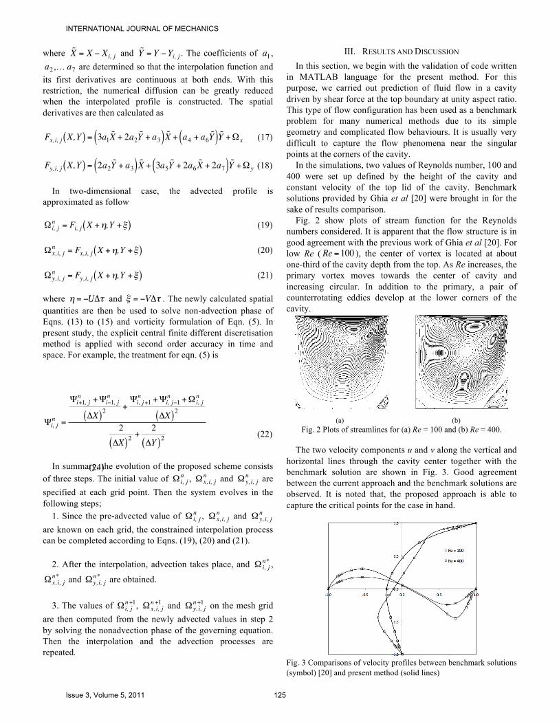
in MATLAB language for the present method. For this purpose, we carried out prediction of fluid flow in a cavity driven by shear force at the top boundary at unity aspect ratio. This type of flow configuration has been used as a benchmark problem for many numerical methods due to its simple geometry and complicated flow behaviours. It is usually very difficult to capture the flow phenomena near the singular points at the corners of the cavity.

In the simulations, two values of Reynolds number, 100 and 400 were set up defined by the height of the cavity and constant velocity of the top lid of the cavity. Benchmark solutions provided by Ghia et al [20] were brought in for the sake of results comparison.

Fig. 2 show plots of stream function for the Reynolds numbers considered. It is apparent that the flow structure is in good agreement with the previous work of Ghia et al [20]. For low Re (

€

Re = 100 ), the center of vortex is located at about one-third of the cavity depth from the top. As Re increases, the primary vortex moves towards the center of cavity and increasing circular. In addition to the primary, a pair of counterrotating eddies develop at the lower corners of the cavity.

(a) (b)

Fig. 2 Plots of streamlines for (a) Re = 100 and (b) Re = 400.

The two velocity components u and v along the vertical and horizontal lines through the cavity center together with the benchmark solution are shown in Fig. 3. Good agreement between the current approach and the benchmark solutions are observed. It is noted that, the proposed approach is able to capture the critical points for the case in hand.

Fig. 3 Comparisons of velocity profiles between benchmark solutions (symbol) [20] and present method (solid lines)



Once we obtained confidence in our proposed method, we

then extend numerical simulation by locating a solid particle in lid-driven cavity flow at shallow conditions. In the present investigation, we only consider one particle in a lid driven cavity and assume the presence of solid particle gives no effect to the fluid flow. The equation of motion for solid particle is written as

€

mpdv pdt

= fp (23)

where

€

mp ,

€

v p and

€

fp are the mass of particle, its velocity and drag force acting on particle due to surrounding fluid respectively. According to Kosinski et al [17], the drag force can be written as follow

€

fp =CDApρu − v p u − v p( )

2 (24)

where

€

Ap is the projected area of solid particle and

€

CD is the drag coefficient which is given as

€

CD =24Rep

(25)

The particle’s Reynolds number in the above equation is

calculated as follow

€

Rep =dp u − v p

υ (26)

where

€

dp is the diameter of solid particle. In summary, the evolution of the scheme consists of three

steps. Once the initial values of

€

u ,

€

v p ,

€

mp and initial position

of solid particle

€

x p , y p( ) are specified, then the system evolves in the following steps.

The drag force acting on solid particles is calculated from Eqn. (24).

Since the pre-calculated value of

€

v pn is known at previous

time step, the new value of particle’s velocity

€

v pn+1 can be

calculated from Eqn. (23) as follow

€

mpv pn+1 − v p

n

Δt= fp (27)

Finally, the new position of solid particle can be determined

as follow

€

x pn+1 = v p

n+1Δt + x pn (28)

(a)

(b)

(c)

Fig. 4 Plot of solid particle trajectories (Bold line) in a shallow lid-driven cavity flow at aspect ratio 2/3 for a) Re = 100, b) Re = 400 and c) Re = 1000. Figs. 4 and 5 show the trajectories a solid particle suspended in two shallow cavities of 2/3 and 1/2. As can be seen from the figures, at low Reynolds number (Re = 100), the particle immediately spirals outwards the center on the cavity. However, for the simulation at higher Reynolds number (Re = 400), the particle firstly make a small spiral near the upper right of the cavity and then gradually spiral outwards the center of the cavity. An interesting phenomenon can be seen



for the simulation at the highest value of Reynolds number and smaller aspect ratio in the present study where the particle eventually drifts and resides in the secondary and weaker vortex.

(a)

(b)

(c)

Fig. 5 Fig. 4 Plot of solid particle trajectories (Bold line) in a shallow lid-driven cavity flow at aspect ratio 1/2 for a) Re = 100, b) Re = 400 and c) Re = 1000.

Fig. 6 shows the transient behavior of vortices in the cavity at aspect ratio of 1/2. The snapshots were taken at seven different dimensionless times; 1s, 2s, 3s, 4s, 10s, 30s, 60s and 70s. As can be seen from the figure, the trajectories of the solid particle significantly affected by the structure of the fluid vortex.

Fig. 6 Location of particle in the flow field at time (from top) 1s, 2s, 3s, 4s, 10s, 30s, 60s, and 70s.



IV. CONCLUSION Numerical computations of solid particle flow in lid-driven

cavity flow were performed using the coupled constrained-interpolated profile method and Lagrangian scheme. The computed results were firstly validated by comparisons of the fluid structure and velocity profiles inside a square cavity. Then the simulations were extended by inclusion of a solid particle in a cavity at shallow conditions. Results from figures 5 and 6 clearly indicate the influence of vortex structure on the particle’s trajectories in the cavity. These demonstrate the capability and the multidisciplinary applications of the present numerical scheme.

REFERENCES [1] G. B. Jeffery, “The motion of ellipsoidal particles immersed in a viscous

fluid”, Proceedings of the Royal Society of London, pp. 161-179, 1922. [2] C. M. White, “The equilibrium of grains on the bed of a stream”,

Proceedings of the Royal Society of London. Mathematical Physical Sciences, pp. 332-338, 1940.

[3] K. R. Oliver and V. G. Jenson, “The inclined settling of dispersed suspensions of spherical particles in square-section tubes”, Canadian Journal of Chemical Engineering, vol. 42, pp. 191-195, 1964.

[4] M. J. Vogel, A. H. Hirsa and J. M. Lopez, “Spatio-temporal dynamics of a periodically driven cavity flow”, Journal of Fluid Mechanics, vol. 478, pp. 197-226, 2003.

[5] O. J. Ilegbusi and M. D. Mat, “A comparison of predictions and measurements of kinematic mixing of two fluids in a 2D enclosure”, Applied Mathermatics Modelling, vol. 24, pp. 199-213, 2000.

[6] L. M. Portela and R. V. A. Oliemans, “Eulerian-Lagrangian DNS/LES of particle-turbulence interactions in wall-bounded flows”, International Journal for Numerical Methods in Fluids, vol. 43, pp. 1045-1065, 2003.

[7] J. Bonet, S. Kulasegaram, M. X. Rodriguez-Paz and M. Profit, “Variational formulation for the smooth particle hydrodynamics (SPH) simulation of fluid and solid problems”, Computer methods in Applied Mechanics and Engineering, vol. 193, pp. 1245-1256, 2004.

[8] B. Oesterle and A. Petitjean, “Simulation of particle-to-particle interactions in gas-solid flows”, International Journal of Multiphase Flow, vol. 19, pp. 199-211, 1993.

[9] S. J. Tsorng, H. Capart, J. S. Lai and D. L. Young, “Three-dimensional tracking of the long time trajectories of suspended particles in a lid-driven cavity flow”, Experiments in Fluids, vol. 40, pp. 314-328, 2006.

[10] R. J. Adrian, “Particle-imaging techniques for experimental fluid mechanics”, Annual Review in Fluid Mechanics, vol. 23, pp. 261-304, 1991.

[11] M. Han, C. Kim, M. Kim and S. Lee, “Particle migration in tube flow of suspensions”, Journal of rheology, vol. 43, no. 5, pp. 1157-1174, 1999.

[12] J. P. Matas, J. F. Morris and E. Guazzelli, “Inertial migration of rigid spherical particles in Poiseuille flow”, Journal of Fluid Mechanics, vol. 515, pp. 171-195, 2004.

[13] S. Ushijima and N. Tanaka, “Three-dimensional particle tracking velocimetry with laser-light sheet scannings”, Journal of Fluid Engineering, vol. 118, pp. 352-357, 1996.

[14] K. Ide and M. Ghil, “Extended Kalman filtering for vortex systems. Part 1. Methodology and point votices”, Dynamics of Atmospheres and Oceans, vol. 27, pp. 301-332, 1997.

[15] C. C. Hu, “Analysis of motility for aquatic sperm in videomicroscopy”, MSc Thesis, National Taiwan University, 2003.

[16] J. I. Liao, “Trajectory and velocity determination by smoother”, MSc Thesis, National Taiwan University, 2002.

[17] P. Kosinki, A. Kosinska and A. C. Hoffmann, “Simulation of solid particles behavior in a driven cavity flow”, Powder Technology, vol. 191, pp. 327-339, 2009.

[18] C. G. Ilea, P. Kosinski and A. C. Hoffmann, “Three-dimensional of a dust lifting process with varying parameters”, International Journal of Multiphase Flow, vol. 34, pp. 869-878, 2008.

[19] C. G. Ilea, P. Kosinski and A. C. Hoffmann, “Simulation of a dust lifting process with rough walls”, Chemical Engineering Science, vol. 63, pp. 3864-3876, 2008.

[20] U. Ghia, K. N. Ghia and C. Y. Shin, “High-Re Solutions for Incompressible Flow using the Navier-Stokes Equations and a Multigrid

Method,” Journal of Computational Physics, vol. 48, no. 1, pp. 387-411, 1982.

Nor Azwadi Che Sidik received the B.Eng. degree from Kumamoto University, Japan in 2001, the M.Sc. degree from University of Manchester Institute of Science and Technology, U.K., in 2003, and the PhD from Keio University, Japan, in 2007. Currently a Senior Lecturer at the Faculty of Mechanical Engineering (under the department of thermofluid), Universiti Teknologi Malaysia.

He has more than 50 publications in reputed international and national journals/conferences. His current research interests include simulation and modeling of thermal fluid flow, fluid structure interaction, numerical methods and advanced engineering mathematical theory. Seyed Mohamad Reza Attarzadeh received B.Sc.(Hons) degree in Mechanical Engineering from The University of Engineering and Technology, Pakistan in 2009. Currently he is a postgraduate student at the Faculty of Mechanical Engineering, Universiti Teknologi Malaysia.

His current research interests include simulation and modeling of fluid flow accompanied with Biomedical application, fluid structure interaction, Micro-Nano heat transfer, numerical methods and advanced engineering mathematics theory.



An accurate numerical prediction of solid particle fluid flow in a lid-driven cavity · ·...

Documents

Transcript of An accurate numerical prediction of solid particle fluid flow in a lid-driven cavity · ·...