An accurate adaptive solver for surface-tension …gfs.sourceforge.net/papers/tension.pdfAn accurate...

An accurate adaptive solver forsurface-tension-driven interfacial flows

Stéphane Popinet

National Institute of Water and Atmospheric ResearchP.O. Box 14-901, Kilbirnie, Wellington, New Zealand

Email: [email protected]

April 2, 2009

Abstract

A method combining an adaptive quad/octree spatial discretisation, geometrical Volume-Of-Fluid interface representation, balanced-force continuum-surface-force surface tension formulationand height-function curvature estimation is presented. The extension of these methods to thequad/octree discretisation allows adaptive variable resolution along the interface and is described indetail. The method is shown to recover exact equilibrium (to machine accuracy) between surface-tension and pressure gradient in the case of a stationary droplet, irrespective of viscosity and spatialresolution. Accurate solutions are obtained for the classical test case of capillary wave oscillations.An application to the capillary breakup of a jet of water in air further illustrates the accuracy andefficiency of the method. The source code of the implementation is freely available as part of theGerris flow solver.

1

AMS: 65M50; 76D05; 76D25; 76D45; 76M12; 76T10

Keywords: Adaptive mesh refinement; Surface tension; Navier-Stokes equations; Height-Function;Parasitic currents; Volume-Of-Fluid; Octree

1 Introduction

Flows of immiscible fluids are ubiquitous in Nature: waves on the sea, waterfalls, raindrops or a garden sprinkler are familiar examples. In general air-water flows exhibit thetypical features associated with many important two-phase-flow phenomena: relatively largedensity ratios, high surface-tension and low viscosity at practical length scales. Furthermoremost of these flows tend to generate complex and evolving interface geometries on spatialscales ranging over several orders of magnitude. This is true not only of obviously complexphenomena such as wave breaking or jet atomisation, but also of the apparently simplersub-phenomena such as jet/droplet breakup and coalescence.

Numerical methods using an implicit representation of the interface such as Volume-Of-Fluid (vof) [1, 2, 3, 4] or Levelset (ls) [5, 6, 7, 8, 9, 10, 11, 12, 13] can robustly and efficientlyrepresent evolving, topologically complex interfaces. The accurate representation of surfacetension within these methods is typically more delicate than for schemes using an explicitrepresentation of the interface [14, 15, 16, 17] and care must be taken to avoid any imbalancebetween discrete surface tension and pressure gradient terms [18, 19, 15, 20, 21, 22, 23]. Forvof methods the accurate evaluation of the geometrical properties of the interface such ascurvature is also an active research topic [24, 21, 25, 23, 26]. Finally dynamic mesh-adaptivemethods can deal efficiently with phenomena involving a wide range of spatial scales [27,28, 29, 6, 7, 30, 8, 31, 17, 9, 32, 33, 34].

In the following I will describe a new combination of a vof and quad/octree adaptive meshrefinement method. The basis for the scheme is the adaptive, incompressible quad/octreeGerris solver described in [35]. It is coupled with a classical geometrical vof scheme whichis generalised to work on the quad/octree in order to allow variable spatial resolution alongthe interface. This is in contrast with many previous implementations of adaptive methodswith vof or ls which restricted adaptivity to regions away from the interface (i.e. resolutionalong the interface was kept constant) [28, 7, 36, 30, 8, 31, 37, 9, 38, 39, 33, 40]. A recentarticle by Malik et al [41] describes a two-dimensional quadtree implementation allowingvariable resolution along the interface but their study is limited to the advection problem(not coupled to the momentum equation). Block-structured amr and levelset methods wereused in [6, 29] to provide variable resolution along the interface. Here we present a novelquad/octree discretisation.

Surface tension representation draws on the “balanced-forced” continuum surface force (csf)concept introduced by Renardy and Renardy [21] and Francois et al [23], coupled with aheight-function (hf) curvature calculation [42, 25] generalised for the quad/octree. Theclassical hf curvature calculation becomes inconsistent at low interface resolution. This isaddressed by a generalised version of the hf curvature concept.

The robustness and accuracy of the generalised surface-tension method is assessed for clas-sical test cases: curvature estimates, stationary droplet with surface tension, capillary waves

2 Section 1

and rising bubbles and compared with published results from other methods. Particularattention is paid to the issue of “parasitic currents” around a stationary droplet [18, 15,23, 43, 26, 40], and we improve upon existing methods by enabling a unique combinationof varying resolution along the interface, improved height-function curvature discretisationand a balanced-force approach. Finally the method is applied to the adaptive solution ofthe surface-tension-driven breakup of a three-dimensional cylindrical jet of water in air.

The full implementation of the method as well as most of the test cases presented in thisarticle are available under the General Public License on the Gerris web site [44, 45].

2 Numerical scheme

The numerical scheme is a direct extension of the scheme described in [35]. Consequently Iwill only give a summary of the elements of the method which are not specific to the Volume-Of-Fluid and surface tension implementations. Details regarding the quad/octree spatialdiscretisation, multilevel Poisson solver, approximate projection and momentum advectionscheme can be found in [35].

2.1 Temporal discretisation

The incompressible, variable-density, Navier–Stokes equations with surface tension can bewritten

ρ (∂tu + u ·∇u)=−∇p+ ∇ · (2 µ D)+ σκ δs n,

∂tρ + ∇ · (ρ u)= 0,

∇ ·u = 0,

with u = (u, v, w) the fluid velocity, ρ ≡ ρ(x, t) the fluid density, µ ≡ µ(x, t) thedynamic viscosity and D the deformation tensor defined as Dij≡ (∂iuj +∂jui)/2. The Diracdistribution function δs expresses the fact that the surface tension term is concentrated onthe interface; σ is the surface tension coefficient, κ and n the curvature and normal to theinterface.

For two-phase flows we introduce the volume fraction c(x, t) of the first fluid and define thedensity and viscosity as

ρ(c)≡ c ρ1 + (1− c) ρ2, (1)

µ(c)≡ c µ1 + (1− c) µ2, (2)

with ρ1, ρ2 and µ1, µ2 the densities and viscosities of the first and second fluids respectively.Field c is either identical to c or is constructed by applying a smoothing spatial filter toc. Using a smoothed field to define the viscosity was found to improve the results for someof the test cases I studied. Unless otherwise specified spatial filtering is not used in the

Numerical scheme 3

applications presented in the following. When spatial filtering is used, field c is constructedby averaging the four (respectively eight in 3d) corner values of c obtained by bilinearinterpolation from the cell-centred values. When spatial filtering is used, the propertiesassociated with the interface are thus “smeared” over three discretisation cells.

The advection equation for the density can then be replaced with an equivalent advectionequation for the volume fraction

∂tc +∇ · (c u)= 0.

A staggered in time discretisation of the volume-fraction/density and pressure leads to thefollowing formally second-order accurate time discretisation

ρn+

1

2

[

un+1−un

∆t+ u

n+1

2

·∇un+

1

2

]

=−∇pn+

1

2

+ ∇ ·[

µn+

1

2

(Dn + Dn+1)]

+ (σ κ δs n)n+

1

2

,

cn+

1

2

− cn−

1

2

∆t+ ∇ · (cn un) =0,

∇ ·un = 0

This system is further simplified using a classical time-splitting projection method [46]

ρn+

1

2

[

u⋆−un

∆t+u

n+1

2

·∇un+

1

2

]

= ∇ ·[

µn+

1

2

(Dn + D⋆)]

+ (σκ δs n)n+

1

2

, (3)

cn+

1

2

− cn−

1

2

∆t+ ∇ · (cn un)= 0, (4)

un+1 = u⋆− ∆t

ρn+

1

2

∇pn+

1

2

, (5)

∇ ·un+1 =0

which requires the solution of the Poisson equation

∇ ·[

∆t

ρn+

1

2

∇pn+

1

2

]

= ∇ ·u⋆ (6)

This equation is solved using the quad/octree-based multilevel solver described in detail in[35]. The iterative solution procedure is stopped whenever the maximum relative change inthe volume of any discretisation element (due to the remaining divergence of the velocityfield) is less than a given threshold γp. Unless otherwise specified this threshold is set to

10−3. The number of Gauss–Seidel relaxations per level is set to four.

It is well-known that the standard multigrid scheme can exhibit slow convergence in thecase of elliptic equations with discontinuous coefficients and/or source terms [47, 48, 49].Depending on the problem and interface topology, this can lead to an important degradationof performance for large-density-ratio flows. While this was not an issue for the applications

4 Section 2

presented in this paper, it is an aspect of the method which warrants further improvements.

The discretised momentum equation (3) can be re-organised as

ρn+

1

2

∆tu⋆ − ∇ ·

[

µn+

1

2

D⋆

]

= ∇ ·[

µn+

1

2

Dn

]

+ (σ κ δs n)n+

1

2

+ ρn+

1

2

[

un

∆t−

un+

1

2

·∇un+

1

2

]

(7)

where the right-hand-side depends only on values at time n and n + 1/2. This is anHelmholtz-type equation which can be solved using a variant of the multilevel Poisson solver.The resulting Crank–Nicholson discretisation of the viscous terms is formally second-orderaccurate and unconditionally stable. The criterion for convergence of the multilevel solveris the relative error γu in each component of the velocity field. Unless otherwise specifiedthis threshold is set to 10−6. The number of Gauss–Seidel relaxations per level is set to four.

The velocity advection term un+

1

2

·∇un+

1

2

is estimated using the Bell–Colella–Glaz second-

order unsplit upwind scheme [50, 35]. This scheme is stable for cfl numbers smaller thanone.

2.2 Spatial discretisation

Space is discretised using a graded quadtree partitioning (octree in three dimensions). Werefer the reader to [35] and references therein for a more detailed presentation of this datastructure and just give a summary of the definitions necessary for the description of thealgorithms presented in this article:

Root cell. The base of the cell tree. The root cell does not have a parent cell and all cellsin the tree are descendants of the root cell.

Children cells. The direct descendants of a cell. Cells other than leaf cells have fourchildren in two dimensions (quadtree) and eight in three dimensions (octree).

Parent cell. The direct ancestor of a given cell.

Leaf cells. The highest cells in the cell tree. Leaf cells do not have children.

Cell level. By convention the root cell is at level zero and each successive generationincreases the cell level by one.

Coarser cell. Cell A is coarser than cell B if level(A) < level(B) and conversely for finercells.

All the variables (components of the momentum, pressure and passive tracers) are collocatedat the centre of each square in 2d (resp. cubic in 3d) discretisation volume. Consistentlywith a finite-volume formulation, the variables are interpreted as the volume-averaged valuesfor the corresponding discretisation volume. The choice of a collocated definition of allvariables makes momentum conservation simpler when dealing with mesh adaptation [35].It is also a necessary choice in order to use the Godunov momentum advection scheme ofBell, Colella and Glaz [50], and it simplifies the implementation of the Crank–Nicholsondiscretisation of the viscous terms; however one has to be careful to avoid the classic problemof decoupling of the pressure and velocity field.

Numerical scheme 5

To do so, an approximate projection method [51, 35] is used for the spatial discretisation ofthe pressure correction equation (5) and the associated divergence in the Poisson equation(4). In a first step the auxiliary cell-centred velocity field u⋆

c is computed using equation

(7). An auxiliary face-centred velocity field u⋆f is then computed using averaging of the cell-

centred values on all the faces of the Cartesian discretisation volumes. When faces are atthe boundary between different levels of refinement of the quad/octree mesh, averaging isperformed so as to guarantee consistency of the corresponding volume fluxes (see [35] fordetails).

The divergence of the auxiliary velocity field appearing on the right-hand-side of equation(6) is then computed for each control volume as the finite-volume approximation

∇ ·u⋆ =1

∆

∑

f

u⋆f ·nf ,

with nf the unit normal vector to the face and ∆ the length scale of the control volume.

After solving equation (6), the pressure correction is applied to the face-centred auxiliaryfield

un+1f = u⋆

f − ∆t

ρn+

1

2

f∇fp

n+1

2

, (8)

where ∇f is a simple face-centred gradient operator (consistent at coarse/fine volume

boundaries, see section 4.1 of [35]). The resulting face-centred velocity field un+1f is exactly

non-divergent by construction.

The cell-centred velocity field at time n +1 is obtained by applying a cell-centred pressurecorrection

un+1c = u⋆

c −∣

∣

∣

∣

∣

∣

∆t

ρn+

1

2

f∇fp

n+1

2

∣

∣

∣

∣

∣

∣

c

, (9)

where the ||c operator denotes averaging over all the faces delimiting the control volume.The resulting cell-centred velocity field un+1

c is approximately divergence-free.

The Poisson equation (6), advection–diffusion equation (7) and pressure corrections (8)

and (9) require an estimate of the face-centred values of the density ρn+1/2f or viscosity

µn+1/2f . Both quantities are obtained using the volume-fraction-weighted averages (1) and

(2) which in turn requires an estimate of cn+1/2f . This face-centred volume fraction is

estimated using a simple average of the cell-centred values in the case of neighbouring cellsat the same level. At fine–coarse and coarse–fine boundaries a second-order interpolationstencil is used, identical to the stencil used to evaluate the face-centred gradient operator∇f (see section 4.1 of [35]). Other choices are possible, including a local face-centred vof

6 Section 2

reconstruction which would eliminate the smoothing effect of the interpolation stencil atcoarse–fine boundaries. Preliminary tests suggest that the interpolation procedure workswell in practice however.

3 Volume Of Fluid advection scheme

To solve the advection equation (4) for the volume fraction we use a piecewise-lineargeometrical Volume Of Fluid (vof) scheme [4] generalised for the quad/octree spatial dis-cretisation. Geometrical vof schemes classically proceed in two steps:

1. Interface reconstruction2. Geometrical flux computation and interface advection

3.1 Interface reconstruction

In a piecewise-linear vof scheme the interface is represented in each cell by a line (resp.plane in three dimensions) described by equation

m ·x =α, (10)

where m is the local normal to the interface and x is the position vector. Given m andthe local volume fraction c, α is uniquely determined by ensuring that the volume of fluidcontained in the cell and lying below the plane is equal to c. This volume can be computedrelatively easily by taking into account the different ways a square (resp. cubic) cell canbe cut by a line (resp. plane) which leads to matched linear and quadratic (resp. cubic)functions of α. This step has been described in detail in several papers [19, 52]. In whatfollows we will assume that given a normal m, a volume fraction c and coefficient α ofequation (10) defined in a coordinate system with origin at the cell centre and in which thecell size is unity, we have the relations:

c =V(m, α),

α =V−1(m, c).

In practice, we use the V and V−1 routines implemented by Ruben Scardovelli, based onanalytical formulae for the solution of quadratic (resp. cubic) equations [52]. The routines

have been well tested and are free from inconsistencies (such as V(m,V−1(m, c))� c) whichmay occur due to round-off errors in limiting cases.

A number of schemes have been proposed for interface normal estimation [4, 53, 54]. Mostof these schemes only require information in a compact neighbourhood of the cell considered:typically a 3× 3 (resp. 3× 3× 3) regular Cartesian stencil. Given this stencil, the methodsuse finite-difference estimates and/or minimisation techniques and return an estimate form. Generalising this approach to a quad/octree discretisation is trivial if the interfacial

Volume Of Fluid advection scheme 7

region (i.e. the compact neighbourhood) is resolved with a constant resolution. In this casethe local discretisation simply reduces to a regular Cartesian discretisation [30, 31, 36].

In order to generalise the method to variable spatial resolution along the interface, we needto be able to reconstruct a local regular Cartesian stencil when cells in the compact neigh-bourhood vary in size. For the sake of clarity we describe the stencil-computation algorithmfor two-dimensional quadtrees. The extension to three dimensions is straightforward.

Given a reference cell C centred on x0, of size ∆, and containing the interface (0 < c < 1),the stencil-computation algorithm proceeds as follows:

Algorithm 1 Stencil computation (C)

1. set X (1, 0), Y (0, 1).2. for each position xi,j x0 +∆ (i X + j Y), − 1 6 i 6 1, − 1 6 j 6 1

a) locate the smallest cell N of size larger than or equal to ∆ containing xi,j

b) set the stencil volume fraction ci,j to the volume fraction of a (virtual) cell N∆ ofsize ∆, centred on xi,j and entirely contained in N

Step 1.2.a of the algorithm is performed using a conditional traversal of the quadtree startingfrom the root cell and stopping whenever either a leaf cell is reached or the size of the cellis equal to ∆. This leads to an efficient point-location algorithm with cost of order O(logn)where n is the number of leaf cells in the quadtree.

For step 1.2.b, several cases must be considered:

Algorithm 2 Equivalent volume fraction (C,xi,j,N)

1. the size of N is equal to the size of C, then N∆ =N and ci,j is simply set to the value ofthe volume fraction in cell N

2. the size of N is larger than ∆ (i.e. N is a coarse neighbour of C and is also a leaf cell)a) N does not contain the interface: ci,j is set to the volume fraction in cell N ( 0 or 1)b) N contains the interface: by definition N∆ does not exist in this case and the equi-

valent volume fraction ci,j needs to be computed from the interface reconstructed incell N

Note that in case 2.1, cell N is not necessarily a leaf cell, however consistent values forthe volume fraction can easily be defined on all levels of the quadtree. This is done beforeinterface reconstruction by traversing the quadtree from the leaf cells to the root cell andsetting the volume fractions of non-leaf cells to the average of their children’s volumefractions.

For the treatment of case 2.2.b, we will assume that the equation m ·x = αN is known forthe fragment of interface contained in cell N . In order to be able to compute the equivalentvolume fraction of the virtual cell N∆ using function V , we need to transform the interfaceequation into the coordinate system centred onN∆. The coordinate transformation is simply

x′ =n ∆ x+ xN −xi,j

∆, (11)

8 Section 3

where n ∆ and xN are the size and position of cell N . The interface equation in thecoordinate system of the virtual cell N∆ is then

m ·x′ = n αN +m

∆· (xN −xi,j), (12)

and the corresponding stencil volume fraction is given by

ci,j =V(m, n αN +m

∆· (xN −xi,j)). (13)

Note that in practice we restrict the quad/octree discretisation so that the sizes of neigh-bouring cells never differ by more than a factor of two [35] i.e. n is always equal to two inthe expressions above.

Once the ci,j stencil has been filled, a standard Cartesian routine for computing the interfacenormal m is called and the interface is reconstructed by evaluating α = V−1(m, c0,0). In

practice we use the Mixed-Youngs-Centred (myc) implementation of Aulisa et al [54] toevaluate m.

As should be clear from the description of algorithm 2, reconstructing an interface in a cellwill require access to the reconstructed interface in any coarser neighbouring cell, howeveraccess to cells finer than the cell considered is never required. Taking this into account, thegeneral interface reconstruction algorithm can be summarised as:

Algorithm 3 Interface reconstruction

1. for each non-leaf cell (traversing from leaf to root)a) set the volume fraction as the average of the children’s volume fractions

2. for each cell C containing the interface (traversing from root to leaf)a) fill the ci,j regular Cartesian stencil using Algorithm 1b) compute m using ci,j and the myc scheme

c) compute α =V−1(m, c0,0)d) store m and α as state variables of cell C

3.2 Interface advection and geometrical flux computation

The basis for volume fraction advection is the direction-split scheme originally implementedby DeBar [55] and re-implemented by others [42, 3, 56]. Considering a single two-dimen-sional Cartesian cell, one timestep of this scheme can be summarised as

c⋆i,j V⋆

i,j = cn−1/2i,j

Vn−1/2i,j + φn−1/2

i−1/2,j − φn−1/2i+1/2,j

, (14)

cn+1/2i,j

Vn+1/2i,j = c⋆

i,jV⋆

i,j + φ⋆i,j−1/2− φ⋆

i,j+1/2, (15)


where V i,j is the effective volume of the cell and φi+1/2,j is the volume flux of the firstphase through the right-hand boundary of the cell (respectively left-hand, top and bottomboundaries for the other indices). The effective volume is defined by taking into accountthe compression or expansion of the cell due to the divergent one-dimensional velocity field,which gives

V⋆i,j ≡ Vn−1/2

i,j + (uni−1/2,j − un

i+1/2,j)∆ ∆t,

Vn+1/2i,j ≡ V⋆

i,j + (uni,j−1/2−un

i,j+1/2)∆ ∆t.

Since the face-centred velocity field unf is discretely non-divergent, the second relation

reduces to Vn+1/2i,j ≡Vn−1/2

i,j ≡∆2. Also, in practice the order of the split advection directions

is reversed at each timestep. In two dimensions, equations (14) and (15) are equivalent tothe Eulerian-implicit and Eulerian-explicit formulations of [53] respectively and the schemeas a whole is identical to the Eulerian-implicit-explicit scheme described by [3]. Exten-sion of this scheme to three dimensions is straightforward.

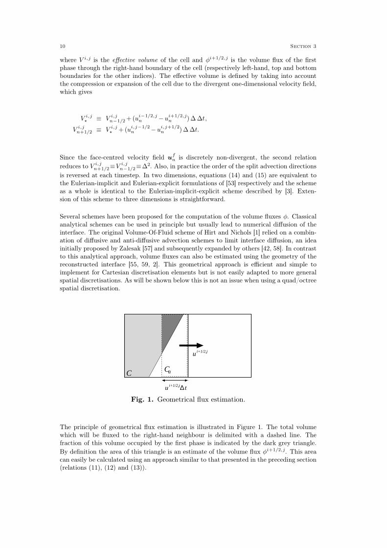
Several schemes have been proposed for the computation of the volume fluxes φ. Classicalanalytical schemes can be used in principle but usually lead to numerical diffusion of theinterface. The original Volume-Of-Fluid scheme of Hirt and Nichols [1] relied on a combin-ation of diffusive and anti-diffusive advection schemes to limit interface diffusion, an ideainitially proposed by Zalesak [57] and subsequently expanded by others [42, 58]. In contrastto this analytical approach, volume fluxes can also be estimated using the geometry of thereconstructed interface [55, 59, 2]. This geometrical approach is efficient and simple toimplement for Cartesian discretisation elements but is not easily adapted to more generalspatial discretisations. As will be shown below this is not an issue when using a quad/octreespatial discretisation.

∆ t

CaC

u

u i+1/2,j

i+1/2,j

Fig. 1. Geometrical flux estimation.

The principle of geometrical flux estimation is illustrated in Figure 1. The total volumewhich will be fluxed to the right-hand neighbour is delimited with a dashed line. Thefraction of this volume occupied by the first phase is indicated by the dark grey triangle.

By definition the area of this triangle is an estimate of the volume flux φi+1/2,j. This areacan easily be calculated using an approach similar to that presented in the preceding section(relations (11), (12) and (13)).

10 Section 3

Ca

Ca

C

Ct

b

t

b

Fig. 2. Special case for geometrical flux computation on a quadtree discret-isation.

Generalising this advection scheme to a quad/octree discretisation only involves dealingwith the special case illustrated in Figure 2. In this case cell C is a coarse cell and eitheror both volume fluxes from C to its finer neighbours are positive. The fluxes then need tobe computed independently for the top- and bottom-halves of the coarse cell (Ct and Cb

in Figure 2). The equation of the interface in both halves can be determined easily usingrelations similar to (11), (12) and (13). Once this is done, calculation of the fluxes in eachhalf-cell is identical to the standard case.

As has been noted before [3], this vof advection scheme is not strictly conservative becausesmall over- or under-shoots of the volume fraction may occur for each direction-sweep.Since interface reconstruction and geometrical flux calculation depend on consistent (i.e.bounded between zero and one) volume fractions, it is necessary to reset any volume fractionviolating this constraint before proceeding to the next direction sweep, which will lead toloss of exact mass conservation. In practice we have found that this scheme is simple toimplement on quad/octrees with mass conservation usually not being an issue, howeverit would be interesting to investigate the extension to quad/octrees of flux-redistributionschemes [3, 56] or exactly mass-preserving geometrical schemes [53, 60].

3.3 Conservation of interface spatial resolution

Depending on the criterion used for spatial adaptivity there may be cases when the interfacespatial resolution could change during interface advection. Given two neighbouring cells Ci

and Ci+1 this would happen whenever the following conditions are met:

1. Ci+1 is coarser than Ci,2. ui+1/2 > 0,3. Ci+1 does not contain the interface (i.e. ci+1 = 0 or ci+1 = 1),4. φi+1/2� ci+1.

In this case the interface fragment contained in cell Ci will be advected to the coarser cellCi+1 resulting in a loss of spatial resolution of the interface.

In order to avoid this problem all cells verifying the conditions above are refined prior tointerface advection for each of the direction sweeps. Initialising the volume fractions of thenew children cells of Ci+1 is trivial since by definition ci+1 = 0 or ci+1 = 1 (condition 3),


however initialising the face-centred velocities uf of the new cells requires some thought.

CC

pv v

p

p pu

u

i+1i

0 1

0

01

31

2

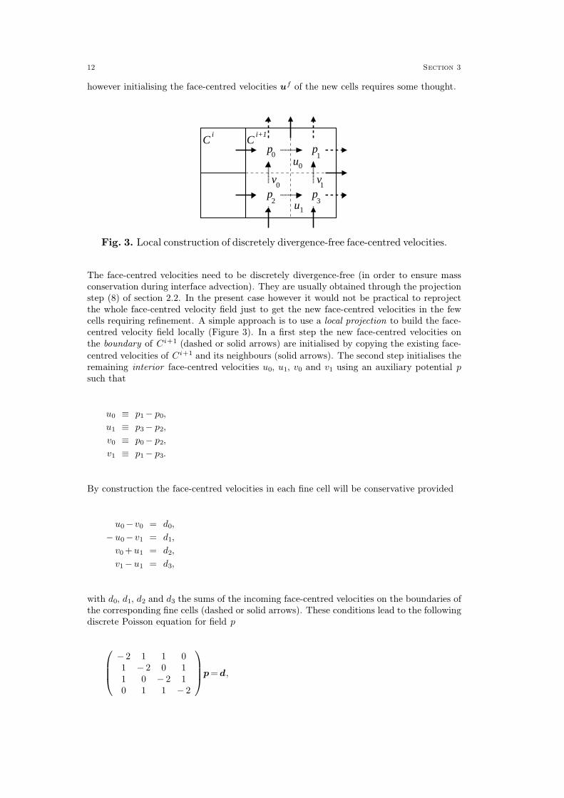
Fig. 3. Local construction of discretely divergence-free face-centred velocities.

The face-centred velocities need to be discretely divergence-free (in order to ensure massconservation during interface advection). They are usually obtained through the projectionstep (8) of section 2.2. In the present case however it would not be practical to reprojectthe whole face-centred velocity field just to get the new face-centred velocities in the fewcells requiring refinement. A simple approach is to use a local projection to build the face-centred velocity field locally (Figure 3). In a first step the new face-centred velocities onthe boundary of Ci+1 (dashed or solid arrows) are initialised by copying the existing face-

centred velocities of Ci+1 and its neighbours (solid arrows). The second step initialises theremaining interior face-centred velocities u0, u1, v0 and v1 using an auxiliary potential p

such that

u0 ≡ p1− p0,

u1 ≡ p3− p2,

v0 ≡ p0− p2,

v1 ≡ p1− p3.

By construction the face-centred velocities in each fine cell will be conservative provided

u0− v0 = d0,

− u0− v1 = d1,

v0 + u1 = d2,

v1− u1 = d3,

with d0, d1, d2 and d3 the sums of the incoming face-centred velocities on the boundaries ofthe corresponding fine cells (dashed or solid arrows). These conditions lead to the followingdiscrete Poisson equation for field p

− 2 1 1 01 − 2 0 11 0 − 2 10 1 1 − 2

p = d,

12 Section 3

which has the solutions

p =

0 0 0 00 3/4 1/4 1/20 1/4 3/4 1/20 1/2 1/2 1

d + arbitrary constant,

provided the solvability condition∑

di = 0 is verified (i.e. the face-centred velocity fieldon the boundary of Ci+1 must be divergence-free). This approach is easily generalised tothree dimensions.

4 Balanced-force surface tension calculation

The accurate estimation of the surface tension term (σ κ δs n)n+

1

2

in the discretised

momentum equation (3) has proven one of the most difficult aspect of the applicationof vof methods to surface-tension-driven flows.

In other methods such as front-tracking (e.g. the “pressure-gradient correction method” of[15]) or levelset coupled with the “ghost fluid method” (gfm) [20], the continuous descriptionof the interface location can be used to derive accurate finite-volume or finite-differenceestimates of the surface-tension and pressure-gradient terms taking into account the dis-continuities at the interface. Unfortunately front-tracking methods cannot deal simply withtopology changes and levelset methods have trouble conserving mass. Coupling vof, levelsetand gfm can be used to overcome the individual drawbacks of each method [23, 61, 43],however this introduces two different representations of the same interface with the associ-ated complexity, efficiency and consistency issues.

In the context of vof methods, the original Continuum-Surface-Force (csf) approach ofBrackbill (1992) proposes the following approximations

σ κ δs n ≈ σ κ ∇c ,

κ ≈ ∇ · n with n ≡ ∇c

|∇c | ,

where c is a spatially-filtered volume fraction field. This approach is known to suffer fromproblematic parasitic currents when applied to the case of a stationary droplet in theoreticalequilibrium [18, 15, 22]. More recently Renardy & Renardy [21] and Francois et al. [23]noted that in this case, since the discretised momentum equation reduces to

−∇pn+

1

2

+σ κ (δs n)n+

1

2

= 0,

Balanced-force surface tension calculation 13

or equivalently using the csf approximation

−∇pn+

1

2

+σ κ (∇c)n+

1

2

= 0, (16)

it is possible to recover exact discrete equilibrium between surface tension and pressuregradient provided:

1. the discrete approximations of both gradient operators in equation (16) are compatible,2. the estimated curvature κ is constant,

then

pn+1/2 =σ κ cn+1/2 + arbitrary constant,

is the exact discrete equilibrium solution. An earlier implementation of a scheme withcompatible pressure and interface gradient operators was also described in [6].

Condition 1 can easily be violated in naive implementations of the csf scheme [62, 23]. Forexample it may seem simpler to compute the surface tension force at the discrete locationswhere the volume fraction is defined. When using a classical staggered discretisation thesurface-tension forces then need to be estimated on the faces of the control volume whichis usually done by averaging the cell-centred estimates. The resulting discrete gradientoperator applied to c in equation (16) is thus a spatially-averaged variant of the discretegradient operator applied to p and condition 1 is violated.

In the present collocated scheme, the cell-centred pressure gradient is computed by aver-aging the face-centred pressure gradients as indicated in equation (9). The correspondingsurface-tension steps verifying condition 1 are:

a) apply the surface-tension force to the auxiliary face-centred velocity field u⋆f as

u⋆f u⋆

f +∆t σ κ

n+1

2

f

ρ(cn+

1

2

f )∇fc

n+1

2

, (17)

b) apply the corresponding cell-centred surface-tension force to u⋆c as

u⋆c u⋆

c +

∣

∣

∣

∣

∣

∣

∆t σ κn+

1

2

f

ρn+

1

2

f∇fc

n+1

2

∣

∣

∣

∣

∣

∣

c

.

These steps are applied immediately before the projection steps. In practice the implementa-tion of steps a) and b) is identical to the implementation of the pressure corrections (8) and(9) respectively. Parameters are used to apply the routines either to cn+1/2 or pn+1/2 with

14 Section 4

weights σ κn+1/2 or − 1 respectively. This avoids duplicating similar code and guaranteesthat condition 1 is verified exactly.

5 Generalised height-function curvature calculation

Condition 2 depends on the accuracy of the curvature estimation. Estimating curvature hastraditionally been the Achilles’ heel of Volume-Of-Fluid schemes and has prompted manyto recommend levelset [5], coupled vof/levelset [63, 64] or front-tracking schemes [15, 16]as alternatives.

Besides the original curvature estimation of Brackbill, several methods have been proposedfor estimating curvature from volume fraction fields. The height-function (hf) curvaturecalculation initially proposed by Torrey et al [65] has recently been shown to give practicalestimates of the curvature which are comparable in accuracy to estimates obtained usingthe differentiation of exact levelset functions [25]. The hf method is also substantiallysimpler to implement than other high-order methods such as parabolic fitting (prost [21])or spline interpolation [24]. An important shortcoming of the standard hf method which israrely discussed, however, is that it becomes inconsistent when the radius of curvature ofthe interface becomes comparable to the mesh size. This case of an under-resolved interfaceoften occurs in practice, particularly when dealing with topology changes.

In the following, I will present a height-function calculation generalised to quad/octreediscretisations and which uses a hierarchy of consistent approximations to deal with thecase of under-resolved interfaces.

5.1 Optimised height-function formulation on quad/octree discretisations

The standard height-function curvature calculation on 2d Cartesian grids [25] can be sum-marised as:

1. Consider a 3 × 7 (resp. 7 × 3) stencil centred on the cell where the curvature is to beevaluated; an estimate of the interface orientation is used to choose the stencil bestaligned with the normal direction to the interface.

2. Build a discrete approximation of the interface height y = h(x) (resp. x = h(y)) bysumming the volume fractions in each column (resp. line).

3. Use finite-difference approximations of the derivatives of the discretised height-functionto compute the curvature

κ =h ′′

(1 + h′2)3/2

∣

∣

∣

∣

∣

x=0

While this scheme could easily be extended to a quad/octree discretisation using theapproach described in section 3.1 (Algorithm 1), it would imply systematically recon-structing a large stencil around each cell where the curvature needs to be evaluated. Inmany cases the stencil does not need to be seven cells high (Figure 4.a) while some casesmay require stencils higher than seven cells in order to obtain a consistent estimate ofthe interface height (Figure 4.b).

Generalised height-function curvature calculation 15

(a) (c)(b)

?

??

?

Fig. 4. (a) A 3 × 3 symmetric stencil is sufficient to obtain a consistentestimate of the interface height for weakly-curved interfaces aligned with thegrid. (b) Symmetric stencils higher than seven cells may be required to obtainconsistent interface heights (here the 9× 3 symmetric stencil indicated by thedotted lines is necessary). More compact asymmetric stencils can be builtindependently for each column (solid lines). (c) In this case only two of thethree interface heights are consistent for either the vertical or the horizontalstencils.

An alternative to using wide symmetric stencils is to build local asymmetric stencils adaptedto the geometry of the interface (in a manner similar to that proposed in [26]). For examplein Figure 4.b local stencils of varying heights can be constructed independently for each ofthe three columns where the interface height is to be evaluated: a 1× 6 stencil for the leftcolumn, a 1× 3 stencil for the central column and a 1× 4 stencil for the right column. Theelementary operation is thus the evaluation of the interface height in a given column, forwhich I propose the following algorithm:

Algorithm 4 Interface height (C, top)

1. set H c(C)2. set N C, ct c(C)3. if ct < 1 then set I true else set I false4. while I = false or N contains the interface

a) replace N with its top neighbour, update ct c(N )b) update H H + ct

c) if N contains the interface then set I true5. if ct� 0 then return inconsistent height6. set N C, cb c(C)7. if cb > 0 then set I true else set I false

16 Section 5

8. while I = false or N contains the interfacea) replace N with its bottom neighbour, update cb c(N )b) update H H + cb

c) if N contains the interface then set I true9. if cb� 1 then return inconsistent height

10. return H and N

C is a cell belonging to the column and can be seen as an initial guess of the position of theinterface. The top and bottom directions used in steps 4.a and 8.a respectively are definedrelative to the interface orientation so that for a consistent interface the cells at the top ofthe column are empty (c = 0) while the cells at the bottom are full (c = 1). In a first stage(steps 2 to 5) volume fractions in the top direction are summed until the interface hasbeen found (I = true) and a full or empty cell has been reached. If the cell which has beenreached is full a consistent stencil cannot be formed and an error is returned (condition 5).In a second stage (steps 6 to 9) the same procedure is repeated in the bottom direction,looking this time for a full cell. Given a good enough initial guess C this algorithm will beequivalent to using optimal local asymmetric stencils. Also, no a priori assumption is madeon the maximum height of the stencil required to obtain a consistent interface height.

Algorithm 4 is easily generalised to a quad/octree discretisation by considering virtualrather than actual cells in a manner similar to Algorithm 1. The virtual cells are constructedon demand when evaluating c(C) and c(N ).

For a given cell C and direction top, the full height-function curvature estimation algorithmcan then be summarised as:

Algorithm 5 Height-function curvature (C, top)

1. set h0 and N0 Interface height (C, top)2. foreach of the 2 (8 in 3d) columns neighbouring C

a) define N as the closest neighbouring (virtual) cell to C in the plane perpendicular tothe top direction

b) set hi and Ni Interface height (N, top)c) set a common origin hi hi + h(Ni)− h(N0)

3. if all heights are consistenta) return the curvature estimated using finite-difference approximations of the deriv-

atives of the discretised height function hi

4. elsea) return all the interface positions deduced from the consistent heights

Step 2.c is necessary since the stencils for each column are formed independently and donot necessarily share a common origin (cf. arrows in Figure 4.b). The function h(C) returnsthe absolute height of the centre of cell C.

5.2 Generalised height-function formulation for under-resolved interfaces

An important drawback of the standard height-function method is that even moderately

Generalised height-function curvature calculation 17

curved interfaces can lead to configurations where consistent interface heights cannot beformed. An example of such a case is given in Figure 4.c where both the standard horizontaland vertical hf curvature estimations fail. The radius of curvature of the interface is 4 ∆which is not a very coarse approximation for many practical applications.

While neither the horizontal nor the vertical stencils on their own can be used to constructa twice-differentiable discrete approximation of the interface height it is clear that a com-bination of all the stencils can allow such an approximation. In the case of Figure 4.c forexample, four average interface positions can be obtained from the consistent interfaceheight estimates (the circles in Figure 4.c). Fitting a curve (e.g. a parabola in 2d, paraboloidin 3d) through these points and differentiating the resulting analytical function will give anestimate of the curvature.

More generally given a cell C and n estimated interface positions {x1,� ,xn}, the followingalgorithm can be used to estimate the curvature

Algorithm 6 Parabola-fitted curvature (C, {x1,� , xn})

1. if the number of independent interface positions is smaller than three (resp. six in 3d)a) a meaningful least-squares fit cannot be achieved, return an error

2. retrieve normal m to the interface in cell C (pre-computed using Algorithm 3)3. compute the coordinates o of the barycentre of the reconstructed interface fragment

contained in C4. define an orthonormal coordinate system R≡{o, (i′, m)} (resp. {o, (i′, j ′,m)} in 3d)

5. compute the transformed coordinates {x1′ ,� , xn

′ } of the interface positions in R6. fit a parabola (resp. paraboloid in 3d) by minimising

F(ai)≡∑

16j6n

[

zj′ − f(ai, xj

′ )]2

,

with

f(ai, x)≡{

a0 x2 + a1 x + a2 in 2d

a0 x2 + a1 y2 + a2 x y + a3 x+ a4 y + a5 in 3d

7. return the mean curvature at the origin o of R

κ≡

2 a0

(1 + a12)3/2

in 2d

2a0 (1+ a4

2) + a1 (1+ a32)− a2 a3 a4

(1+ a32 + a4

2)3/2in 3d

The condition in step 1 uses the number of independent positions rather than the totalnumber of positions n. Two interface positions a and b are considered independent provided|a − b| > ∆ . This condition ensures that the resulting minimisation problem is well-conditioned. The minimisation only requires the solution of a 3×3 (resp. 6×6 in 3d) linearsystem.

In practice this scheme is sufficient to compute the curvature in most cases where the

18 Section 5

standard hf technique fails, however the number of independent positions – given by con-sistent interface height estimates – may become too small for complicated interfaces at verycoarse resolutions. In this case a new set of interface positions is constructed by computingthe coordinates of the barycentres of the reconstructed interface fragments in each cellof a 3 × 3 stencil (resp. 3 × 3 × 3 in 3d). If this approach in turn fails to provide enoughindependent positions, the cell considered most probably contains an isolated/degenerateinterface fragment and the curvature is simply set to zero.

The overall algorithm for computing the interface mean curvature in a cell C containing theinterface can then be summarised as

Algorithm 7 curvature (C)

1. retrieve normal m to the interface in cell C (pre-computed using Algorithm 3)2. compute a set S of two (resp. three in 3d) spatial directions in decreasing order of

alignment with normal m

3. foreach top direction in Sa) compute κ =Height-function curvature (C, top)b) if κ is consistent return κ

c) else add the interface positions deduced from the consistent heights to set I4. if the number of independent positions in I is smaller than three (resp. six in 3d)

a) replace I with the set of interface positions built from the barycentres of the recon-structed interface fragments in a 3× 3 (resp. 3× 3× 3 in 3d) stencil centred on C

b) if the number of independent positions in I is still too small return zero5. return Parabola-fitted curvature (C, I)

The algorithm is hierarchical. In the majority of cases it will return within the first iterationof loop 3 (i.e. the standard hf method). In some cases the direction “best-aligned” withnormal m will lead to inconsistent interface heights while the next best direction will notand the algorithm will return after more than one iteration of loop 3. Most other cases willbe dealt with directly by step 5, rarer cases will require step 4.a and still rarer cases step4.b. While estimating curvature using parabola fitting is substantially more expensive thanthe standard hf method, in practice the overall cost is thus largely dominated by the costof the standard hf method.

The balanced-force surface tension correction (17) requires face-centred interface curvatureestimates. The face-centred curvatures are computed either by averaging the cell-centredcurvatures of the neighbouring cells when they both contain the interface, or by taking thevalue of the cell-centred curvature in either cell containing the interface.

6 Results

6.1 Convergence of the generalised height-function curvature

The standard height-function method has been shown to provide asymptotically second-

Results 19

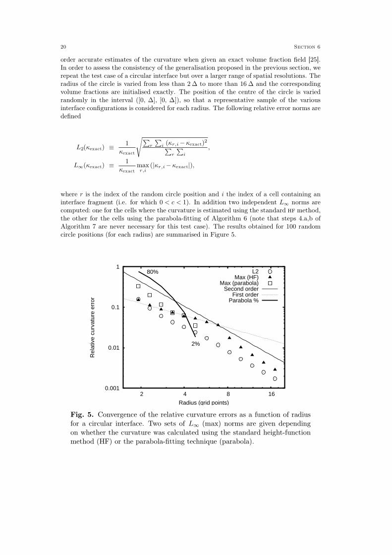
order accurate estimates of the curvature when given an exact volume fraction field [25].In order to assess the consistency of the generalisation proposed in the previous section, werepeat the test case of a circular interface but over a larger range of spatial resolutions. Theradius of the circle is varied from less than 2 ∆ to more than 16 ∆ and the correspondingvolume fractions are initialised exactly. The position of the centre of the circle is variedrandomly in the interval ([0, ∆], [0, ∆]), so that a representative sample of the variousinterface configurations is considered for each radius. The following relative error norms aredefined

L2(κexact) ≡ 1

κexact

∑

r

∑

i(κr,i − κexact)2∑

r

∑

i

√

,

L∞(κexact) ≡ 1

κexactmaxr,i

(|κr,i − κexact|),

where r is the index of the random circle position and i the index of a cell containing aninterface fragment (i.e. for which 0 < c < 1). In addition two independent L∞ norms arecomputed: one for the cells where the curvature is estimated using the standard hf method,the other for the cells using the parabola-fitting of Algorithm 6 (note that steps 4.a,b ofAlgorithm 7 are never necessary for this test case). The results obtained for 100 randomcircle positions (for each radius) are summarised in Figure 5.

0.001

0.01

0.1

1

2 4 8 16

Rel

ativ

e cu

rvat

ure

erro

r

Radius (grid points)

2%

80% L2Max (HF)

Max (parabola)Second order

First orderParabola %

Fig. 5. Convergence of the relative curvature errors as a function of radiusfor a circular interface. Two sets of L∞ (max) norms are given dependingon whether the curvature was calculated using the standard height-functionmethod (HF) or the parabola-fitting technique (parabola).

20 Section 6

The thick curve in the figure indicates the proportion of cases where parabola fitting wasnecessary (from ≈ 80% for a radius of 2 ∆ down to ≈ 2% for a radius of 5 ∆). Above aradius of approximately 5 ∆, the standard hf method is always consistent and use of theparabola-fitting technique is not necessary. In this regime an asymptotically second-orderconvergence in both the L2 and L∞ norms is observed as in previous studies.

At low resolutions the largest errors are obtained for the cases in which the parabola-fittingtechnique is used. This is not surprising since at low resolution the hf method is consistentonly for nearly horizontal or vertical interfaces for which good curvature estimates can befound. The parabola-fitting errors show second-order convergence.

0.001

0.01

0.1

-π -π/2 0 π/2 π

Rel

ativ

e cu

rvat

ure

erro

r

Angle

radius = 4 ∆radius = 13 ∆

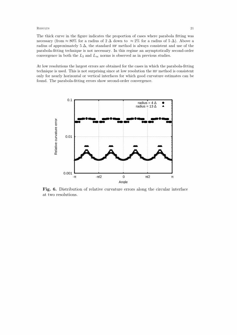
Fig. 6. Distribution of relative curvature errors along the circular interfaceat two resolutions.

Results 21

At intermediate resolutions (radius ≈ 4 ∆) the maximum errors for both methods arecomparable and correspond to cases where the interface is inclined at 45◦ (Figure 6). Inter-estingly, in this regime the L∞ norm of the standard hf method only shows first-orderconvergence.

Over the whole range of resolutions these results are consistent with second-order conver-gence of the generalised height-function technique in both the L2 and L∞ norms.

6.2 Circular droplet in equilibrium

6.2.1 Stationary droplet

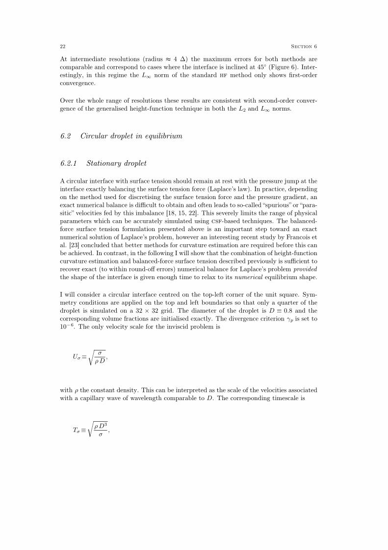
A circular interface with surface tension should remain at rest with the pressure jump at theinterface exactly balancing the surface tension force (Laplace’s law). In practice, dependingon the method used for discretising the surface tension force and the pressure gradient, anexact numerical balance is difficult to obtain and often leads to so-called “spurious” or “para-sitic” velocities fed by this imbalance [18, 15, 22]. This severely limits the range of physicalparameters which can be accurately simulated using csf-based techniques. The balanced-force surface tension formulation presented above is an important step toward an exactnumerical solution of Laplace’s problem, however an interesting recent study by Francois etal. [23] concluded that better methods for curvature estimation are required before this canbe achieved. In contrast, in the following I will show that the combination of height-functioncurvature estimation and balanced-force surface tension described previously is sufficient torecover exact (to within round-off errors) numerical balance for Laplace’s problem providedthe shape of the interface is given enough time to relax to its numerical equilibrium shape.

I will consider a circular interface centred on the top-left corner of the unit square. Sym-metry conditions are applied on the top and left boundaries so that only a quarter of thedroplet is simulated on a 32 × 32 grid. The diameter of the droplet is D ≡ 0.8 and thecorresponding volume fractions are initialised exactly. The divergence criterion γp is set to10−6. The only velocity scale for the inviscid problem is

Uσ ≡ σ

ρ D

√

,

with ρ the constant density. This can be interpreted as the scale of the velocities associatedwith a capillary wave of wavelength comparable to D. The corresponding timescale is

Tσ ≡ ρ D3

σ

√

,

22 Section 6

which is proportional to the period of the capillary wave. For a viscous fluid another times-cale can be defined as

Tν ≡D2/ν ,

with ν the kinematic viscosity. The time it takes for momentum to diffuse across the dropletis proportional to Tν. Finally the ratio of these two timescales is

Tν

Tσ

=σ D

ρ ν2

√

= La√

,

with La the Laplace number.

For our time-explicit discretisation of the surface tension term, numerical stability requiresthat the timestep be smaller than the period of the shortest capillary wave i.e.

∆t 6ρ ∆3

π σ

√

. (18)

1e-16

1e-14

1e-12

1e-10

1e-08

1e-06

1e-04

0.01

0 0.1 0.2 0.3 0.4 0.5 0.6 0.7 0.8 0.9 1

Non

-dim

ensi

onal

RM

S v

eloc

ity

Non-dimensional time

La=120La=1200

La=12000

Fig. 7. Evolution of the rms velocity around a circular droplet in theoreticalequilibrium for different Laplace numbers. Time and velocity are made non-dimensional using Tν and Uσ as reference scales respectively.

Results 23

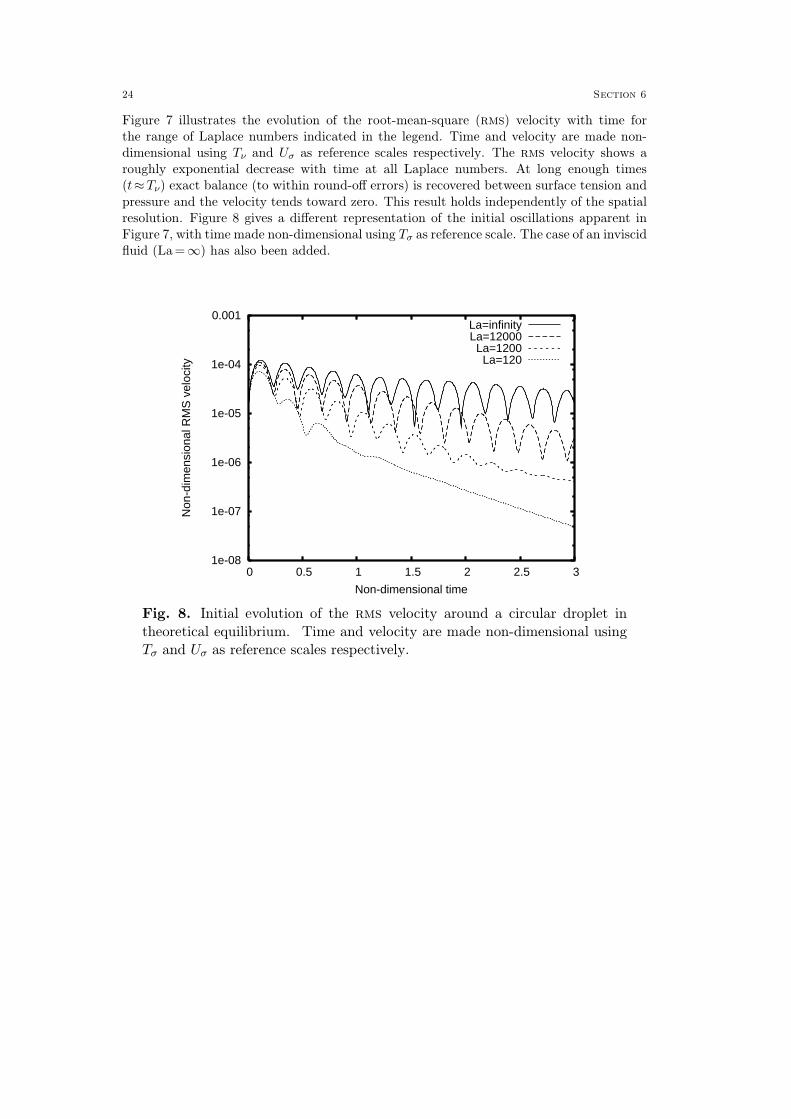
Figure 7 illustrates the evolution of the root-mean-square (rms) velocity with time forthe range of Laplace numbers indicated in the legend. Time and velocity are made non-dimensional using Tν and Uσ as reference scales respectively. The rms velocity shows aroughly exponential decrease with time at all Laplace numbers. At long enough times(t≈Tν) exact balance (to within round-off errors) is recovered between surface tension andpressure and the velocity tends toward zero. This result holds independently of the spatialresolution. Figure 8 gives a different representation of the initial oscillations apparent inFigure 7, with time made non-dimensional using Tσ as reference scale. The case of an inviscidfluid (La=∞) has also been added.

1e-08

1e-07

1e-06

1e-05

1e-04

0.001

0 0.5 1 1.5 2 2.5 3

Non

-dim

ensi

onal

RM

S v

eloc

ity


La=infinityLa=12000La=1200

La=120

Fig. 8. Initial evolution of the rms velocity around a circular droplet intheoretical equilibrium. Time and velocity are made non-dimensional usingTσ and Uσ as reference scales respectively.

24 Section 6

(a) (b)

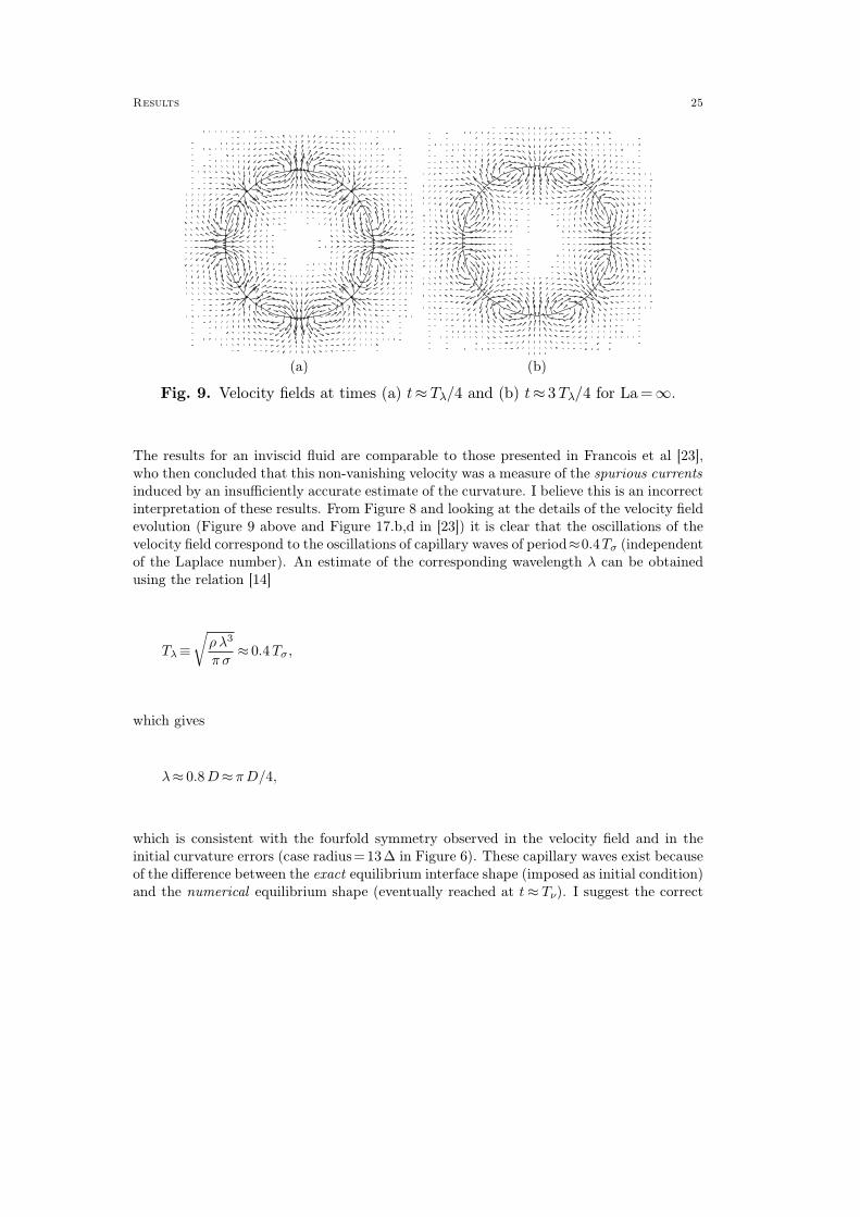
Fig. 9. Velocity fields at times (a) t≈Tλ/4 and (b) t≈ 3 Tλ/4 for La=∞.

The results for an inviscid fluid are comparable to those presented in Francois et al [23],who then concluded that this non-vanishing velocity was a measure of the spurious currentsinduced by an insufficiently accurate estimate of the curvature. I believe this is an incorrectinterpretation of these results. From Figure 8 and looking at the details of the velocity fieldevolution (Figure 9 above and Figure 17.b,d in [23]) it is clear that the oscillations of thevelocity field correspond to the oscillations of capillary waves of period≈0.4Tσ (independentof the Laplace number). An estimate of the corresponding wavelength λ can be obtainedusing the relation [14]

Tλ≡ ρ λ3

πσ

√

≈ 0.4Tσ,

which gives

λ≈ 0.8D≈ πD/4,

which is consistent with the fourfold symmetry observed in the velocity field and in theinitial curvature errors (case radius=13∆ in Figure 6). These capillary waves exist becauseof the difference between the exact equilibrium interface shape (imposed as initial condition)and the numerical equilibrium shape (eventually reached at t ≈ Tν). I suggest the correct

Results 25

interpretation is in fact that the velocity fluctuations observed are the result of a physically-consistent numerical solution of the evolution of a perturbed initial interface shape. Theresulting capillary waves are then exponentially damped by viscosity – again in a physicallyconsistent manner – on timescales of order Tν (with a damping coefficient proportional toν as illustrated by the roughly constant slopes in Figure 7). This is in contrast with whatis usually understood by spurious or parasitic currents which are continuously fed energyby an unphysical unbalance, do not vanish with time and cannot generally be interpretedas consistent physical entities (such as capillary waves).

When the numerical equilibrium interface shape is reached, we expect the estimatedcurvature to be exactly constant so that condition 2 of section 4 is verified. This is indeedthe case as illustrated in Figure 10 where the saturation of the standard deviation atO(10−11) is due to round-off errors.

1e-12

1e-11

1e-10

1e-09

1e-08

1e-07

1e-06

1e-05

1e-04

0.001

0.01

0 0.2 0.4 0.6 0.8 1

Cur

vatu

re s

tand

ard

devi

atio

n


La=120La=1200

La=12000

Fig. 10. Evolution of the standard deviation along the interface of the numer-ical curvature as a function of time for the Laplace numbers indicated in thelegend. Time is made non-dimensional using Tν as reference scale.

Finally the accuracy of the numerical equilibrium solution can be assessed by comparingthe final shape of the interface with the exact equilibrium shape (the initial circular shape).Two measures are used: the relative curvature error |κequilibrium − κexact|/κexact and theshape error defined as

L2(shape) ≡∑

i(ci − ci

exact)2∑

i

√

,

26 Section 6

L∞(shape) ≡ maxi

(|ci − ciexact|),

where cexact is the exact volume fraction field. Figure 11 summarises the convergence ofboth measures when the spatial resolution is varied. Close to second-order convergence isobtained for both measures and the absolute values of the errors are small even at coarseresolutions.

1e-04

0.001

0.01

0.1

4 8 16 32 64

Rel

ativ

e cu

rvat

ure

erro

r


Second order

1e-06

1e-05

1e-04

0.001

0.01

4 8 16 32 64

Sha

pe e

rror


L2Max

Second order

(a) (b)

Fig. 11. Convergence with spatial resolution of two error measures of theequilibrium interface shape. (a) Relative error on the equilibrium curvature:|κequilibrium− κexact|/κexact. (b) L2 and L∞ norms of the shape error.

To conclude, the results presented in this section demonstrate that the combination of abalanced-force csf implementation and a height-function curvature estimation is sufficientto obtain an exact equilibrium solution (for velocity) in the case of a stationary droplet. Thenumerical equilibrium shape obtained is very close to the theoretical equilibrium shape andshows second-order convergence with spatial refinement. The timescale necessary to reachthe numerical equilibrium solution is comparable to the viscous dissipation timescale Tν asexpected from physical considerations. In practice this means that test cases designed toevaluate the accuracy of a given surface tension implementation (for the stationary dropletproblem) need to make sure that simulations are run for timescales comparable to Tν (thiswas not the case in the study of Francois et al. [23]). For shorter timescales the resultsobtained will only reflect the accuracy of the initial curvature estimation. Estimating thisinitial error is better done using a test case similar to that of Section 6.1.

6.2.2 Translating droplet

While the previous test case demonstrates convergence toward the exact velocity solution inthe case of a stationary droplet with surface tension, it is only a weak test of the combinedaccuracy of the interface advection scheme and the surface tension discretisation. In mostpractical applications droplets do not stand still but are advected around by the mean flow.A simple but more representative variant can be built from the previous case by addinga constant, uniform background velocity field. The exact solution in the moving frame ofreference is unchanged but the numerical solution requires advection of the interface across

Results 27

the fixed computational grid. Errors in interface advection will induce fluctuating errors incurvature estimates and hence – through surface tension – in the velocity field. Numerousstudies have considered the case of a stationary droplet with surface tension [18, 15, 21,16, 22, 23] and/or the advection of a circular interface without coupling to the momentumequation [2, 3, 53, 64, 33, 41] but I am not aware of any study using a combination of both,hence the present test case.

The following results are obtained when considering a circular interface of diameter D =0.4contained in the unit square with a mesh refinement equivalent to a 64× 64 regular spatialresolution. Periodic boundary conditions are used in the horizontal direction, symmetryconditions on the top and bottom boundaries. A constant velocity U is initialised in thehorizontal direction. Compared to the previous test case, this introduces a new timescale

TU ≡D/U , with Tσ/TU = We√

and We the Weber number.

0

0.0005

0.001

0.0015

0.002

0.0025

0.003

0 0.1 0.2 0.3 0.4 0.5 0.6 0.7 0.8 0.9 1

Non

-dim

ensi

onal

RM

S v

eloc

ity


La=120La=1200La=12000La=infinity

Fig. 12. Evolution with time of the norm of the velocity in the translatingframe of reference for different Laplace numbers. Time and velocity are madenon-dimensional using TU and U as reference scales respectively.

Figure 12 illustrates the evolution with time of the non-dimensional root-mean-square velo-city – in the translating frame of reference – for different Laplace numbers. The Webernumber is 0.4. Time and velocity are made non-dimensional using TU and U as referencescales respectively. In contrast to the results of the previous section, the velocity does notconverge toward the exact solution with time. The frequency associated with the oscillationsapparent in the figure scales like U/∆. This is due to advection errors continually perturbingthe interface shape and thus the estimated curvature. The amplitude of this “spurious”velocity field is indicative of the accuracy of the combination of: advection scheme, curvatureestimation and surface tension scheme. This simulation was repeated for a range of spatial

28 Section 6

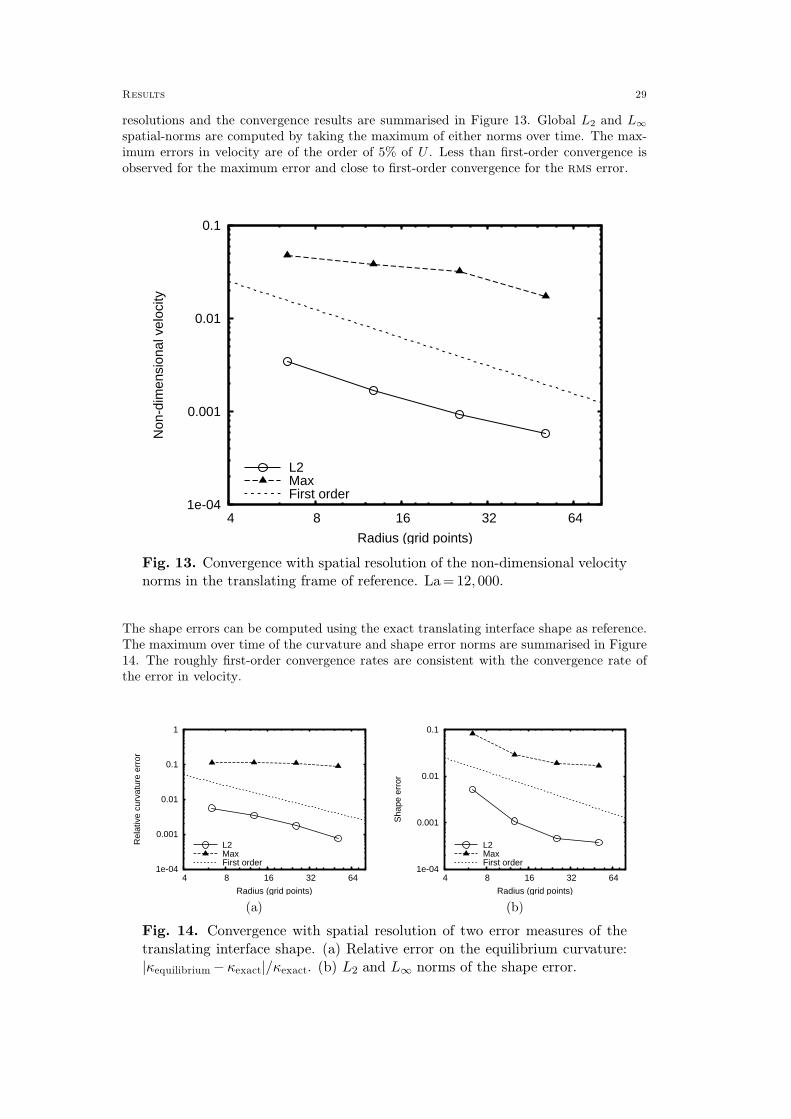
resolutions and the convergence results are summarised in Figure 13. Global L2 and L∞

spatial-norms are computed by taking the maximum of either norms over time. The max-imum errors in velocity are of the order of 5% of U . Less than first-order convergence isobserved for the maximum error and close to first-order convergence for the rms error.

1e-04

0.001

0.01

0.1

4 8 16 32 64

Non

-dim

ensi

onal

vel

ocity


L2MaxFirst order

Fig. 13. Convergence with spatial resolution of the non-dimensional velocitynorms in the translating frame of reference. La= 12, 000.

The shape errors can be computed using the exact translating interface shape as reference.The maximum over time of the curvature and shape error norms are summarised in Figure14. The roughly first-order convergence rates are consistent with the convergence rate ofthe error in velocity.

1e-04

0.001

0.01

0.1

1

4 8 16 32 64

Rel

ativ

e cu

rvat

ure

erro

r


L2MaxFirst order

1e-04

0.001

0.01

0.1

4 8 16 32 64

Sha

pe e

rror


L2MaxFirst order

(a) (b)

Fig. 14. Convergence with spatial resolution of two error measures of thetranslating interface shape. (a) Relative error on the equilibrium curvature:|κequilibrium− κexact|/κexact. (b) L2 and L∞ norms of the shape error.

Results 29

Finally the dependences of the relative error in velocity on the Weber and Laplace numbers

are illustrated in Figure 15.a and 15.b. The relative error scales like We−1/2 or equivalentlylike U−1 (σ being kept constant) which means that the absolute error in velocity is essen-tially independent from U . The relative error in velocity is also seen to be weakly dependenton the Laplace number (Figure 15.b)

1e-04

0.001

0.01

0.1

0.1 1 10 100

Non

-dim

ensi

onal

vel

ocity

Weber

L2MaxWe-1/2

1e-04

0.001

0.01

0.1

10 100 1000 10000N

on-d

imen

sion

al v

eloc

ity

Laplace

L2MaxLa1/6

(a) (b)

Fig. 15. Dependence of the relative error in velocity on: (a) the Webernumber, La = 12, 000, (b) the Laplace number, We = 0.4 . Equivalent res-olution 64× 64.

The convergence toward the exact solution for a stationary droplet presented in the previoussection has been one of the main goals of several recent sophisticated surface tension imple-mentations [21, 16, 23]; however the results obtained in the present section – for a test casemore relevant to real applications – underline the need for yet further advances. An avenueof investigation revealed by the translating droplet test case regards the tighter integration(and coupled evaluation) of the advection and curvature/surface tension schemes.

6.3 Capillary wave

Capillary waves are a basic feature of surface-tension-driven flows and their adequatenumerical resolution is a prerequisite to more complex applications. The small-amplitudedamped oscillations of a capillary wave are a now classical test case of the accuracy ofnumerical schemes for the time-dependent dynamics of viscous, surface-tension-driven two-phase flows [15]. For example a recent study by Gerlach et al. (2006) used this test case toassess the relative accuracies of a range of vof and vof/levelset techniques.

A sinusoidal perturbation is applied to a flat interface between two fluids initially at rest.Under the influence of surface tension the interface oscillates around its equilibrium position.

30 Section 6

The amplitude of the oscillation decays due to viscous dissipation. The solution to thisinitial value problem is significantly different from the normal mode analysis of Lamb [67](which predicts exponentially-damped oscillations) because the finite time of diffusion ofvorticity generated at the interface into each of the phases introduces non-trivial historyterms in the evolution equations. Nonetheless, Prosperetti [68] found an exact analyticalsolution in the limit of vanishingly small amplitudes which can be used as reference.

Prosperetti’s theory is valid for infinite domains and we found that in order to get goodagreement at high resolutions it is necessary to move the top and bottom boundaries farenough away from the interface. Using a [−λ/2, λ/2][− 3 λ/2, 3 λ/2] domain – with λ thewavelength of the perturbation – seems to be sufficient. As in Popinet and Zaleski [15] andGerlach et al. [66] the initial perturbation amplitude is λ/100, the Laplace number 3000 andthe densities and viscosities of both fluids are identical. The timestep is controlled by theexplicit surface-tension stability criterion (18). The typical evolution of the relative max-imum interface elevation over time is illustrated in Figure 16. The normal-mode oscillationfrequency ω0 is defined by the dispersion relation

ω02 =

σ k3

2 ρ,

with k = 2π/λ the wavenumber.

0

0.001

0.002

0.003

0.004

0.005

0.006

0.007

0.008

0.009

0.01

0 5 10 15 20 25

Rel

ativ

e am

plitu

de


ProsperettiThis study

Fig. 16. Time evolution of the relative maximum interface height of a capil-lary wave. La= 3000. Time is made non-dimensional using 1/ω0 as referencetimescale. Equivalent resolution 64× 192.

The error between the theoretical solution of Prosperetti and the numerical solution can be

Results 31

evaluated using the L2 norm

L2≡ 1

λ

ω0

25

∫

t=0

25/ω0

(h− hexact)2

√

,

where h (resp. hexact) is the maximum interface height obtained numerically (resp. theor-etically). Table 1 and Figure 17 summarise the results obtained for: this study, the prost

[21] and clsvof [63] implementations of Gerlach et al [66], the csf implementation ofGueyffier et al [19], the balanced-forced level-set method of Herrmann [40] and the front-tracking method of Popinet and Zaleski [15].

Method/Resolution 8 16 32 64 128

Present study 0.1568 0.0279 0.00838 0.0018 0.000545prost [66] 0.2960 0.0818 0.0069 0.0018 –clsvof [66] 0.3169 0.0991 0.0131 0.0033 –csf [19] – – 0.1168 0.0132 0.007rlsg [40] – 0.1116 0.0295 0.0114 0.0067Front-tracking [15] 0.3018 0.0778 0.0131 0.0082 0.00645

Table 1. Convergence of the L2 error on the maximum interface height ofviscous capillary wave oscillations for different methods. The resolution isgiven in number of grid points per wavelength. ρ1/ρ2=1, µ1/µ2=1, La=3000.

0.0001

0.001

0.01

0.1

1

8 16 32 64 128

L 2 r

elat

ive

erro

r

Number of grid points/wavelength

CSFRLSGCLSVOFFront-trackingPROSTThis studySecond order

Fig. 17. Convergence of the L2 error on the maximum interface height ofviscous capillary wave oscillations for different methods.

32 Section 6

Close to second-order convergence with spatial resolution is obtained for the present study,prost and clsvof. The deviation from second-order convergence for the csf and front-tracking methods at high resolutions may be due to the influence of the top and bottomboundaries (square domains were used in both these studies). The results of the presentmethod are substantially more accurate at low resolutions than the results of the othermethods given in Figure 17 and Table 1. This is important since in practice capillary wavesare often the smallest features of interest and are usually captured at the limit of spatialresolution.

At high resolutions the present method is at least as accurate as prost. The prost methodrelies on systematic parabola-fitting through non-linear minimisation which has beendemonstrated to be very accurate [21] but is also much more computationally expensivethan the present method.

Finally the convergence results for an air/water capillary wave are given in Table 2. Thedensity ratio is 850 and the dynamic viscosity ratio is 55.72. The Laplace number in thedenser fluid is 3000 and the other parameters are identical to the constant density caseabove. The density and viscosity are defined using the filtered field c~ of equations (1) and(2). Although the errors are larger than for the constant density case they are still small andgood convergence is obtained. These results can be compared with the results in the recentstudy by Herrmann [40] (Table 15) which show significantly larger errors and a saturationof convergence for resolutions above 64.

Method/Resolution 8 16 32 64 128

Present study 0.1971 0.0754 0.0159 0.00576 0.00313

Table 2. Convergence of the L2 error on the maximum interface height of vis-cous capillary wave oscillations for parameters corresponding to an air/waterinterface. ρ1/ρ2 = 850, µ1/µ2 = 55.72, La1 = 3000.

6.4 Two-dimensional inviscid rising bubble

An inaccurate representation of surface tension is particularly noticeable for the case of alight gas bubble rising in a dense, low-viscosity fluid [20, 56, 23]. Figure 18 illustrates theresults obtained for one of the cases considered by Francois et al [23]. A two-dimensionalbubble of density 1.226 rises in a fluid of density 1000 due to a downward-acting gravity

Results 33

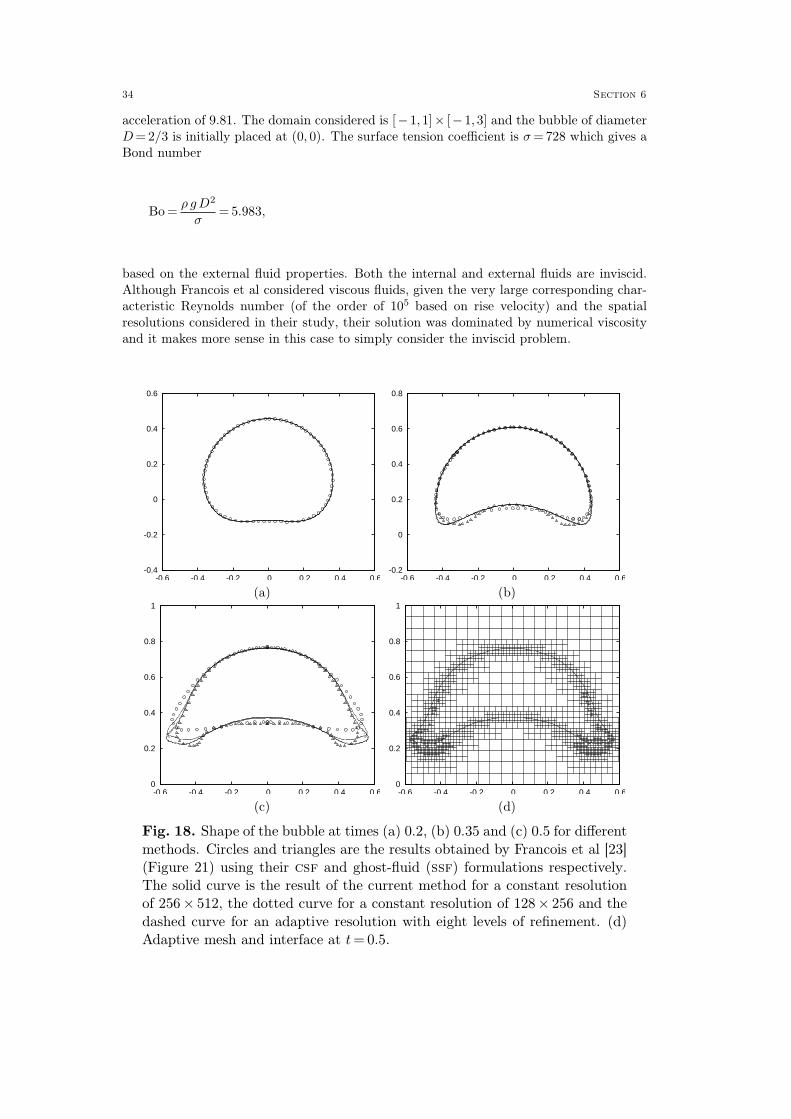
acceleration of 9.81. The domain considered is [−1,1]× [−1,3] and the bubble of diameterD =2/3 is initially placed at (0, 0). The surface tension coefficient is σ = 728 which gives aBond number

Bo=ρ gD2

σ= 5.983,

based on the external fluid properties. Both the internal and external fluids are inviscid.Although Francois et al considered viscous fluids, given the very large corresponding char-acteristic Reynolds number (of the order of 105 based on rise velocity) and the spatialresolutions considered in their study, their solution was dominated by numerical viscosityand it makes more sense in this case to simply consider the inviscid problem.

-0.4

-0.2

0

0.2

0.4

0.6

-0.6 -0.4 -0.2 0 0.2 0.4 0.6-0.2

0

0.2

0.4

0.6

0.8

-0.6 -0.4 -0.2 0 0.2 0.4 0.6

(a) (b)

0

0.2

0.4

0.6

0.8

1

-0.6 -0.4 -0.2 0 0.2 0.4 0.6 0

0.2

0.4

0.6

0.8

1

-0.6 -0.4 -0.2 0 0.2 0.4 0.6

(c) (d)

Fig. 18. Shape of the bubble at times (a) 0.2, (b) 0.35 and (c) 0.5 for differentmethods. Circles and triangles are the results obtained by Francois et al [23](Figure 21) using their csf and ghost-fluid (ssf) formulations respectively.The solid curve is the result of the current method for a constant resolutionof 256× 512, the dotted curve for a constant resolution of 128× 256 and thedashed curve for an adaptive resolution with eight levels of refinement. (d)Adaptive mesh and interface at t= 0.5.

34 Section 6

As is clear from the symbols in Figure 18, Francois et al found that their results weresensitive to the details of the method used for the discretisation of the pressure: circlesymbols for the continuous approach (csf) and triangular symbols for the ghost-fluid sharpinterface approach (ssf). The method described in the present article was applied at dif-ferent resolutions with and without adaptive refinement. The solid line corresponds to theresults obtained on the finest mesh using a constant resolution of 256×512. The dotted linegives the results for a constant resolution of 128× 256 and the dashed line, the results foran adaptive resolution corresponding to an equivalent resolution of 256×512. The adaptiveresults were obtained by controlling the mesh size ∆ so that the vorticity criterion

∆ |∇×u|< 1/2,

was verified at each timestep, with a limit on resolution of eight levels of refinement. Atypical mesh is illustrated on Figure 18.(d). The vorticity generated at the interface isadvected tangentially and accumulates at the stagnation points corresponding to the rearcorners of the bubble. This increase in vorticity along the interface is matched by a corres-ponding increase in spatial resolution along the interface. The number and positions of thetransitions between levels of refinement along the interface vary with bubble motion andshape evolution. This provides a good coverage of the consistency of the surface tensionand curvature estimation schemes on the variable resolution quadtree mesh.

The results at t = 0.2 are identical for all methods and resolutions considered. At t = 0.35the results for the current scheme are identical. They closely match the results of Francoiset al in the front part of the bubble and fall between the csf and ssf results for the rearpart. At t=0.5, the results for the current scheme also fall between the csf and ssf resultsof Francois et al, but the coarse mesh results for the current scheme (dotted line) differfrom the fine mesh results (a resolution dependence also observed by Francois et al). Theconstant fine mesh results and adaptive results are almost identical. This confirms theoverall consistency of the adaptive scheme when resolution varies along the interface, for aflow with strong surface tension, low viscosity and large density ratio.

Resolution # grid points # timesteps cpu time Speed

256× 512 203,161,600 1,550 12,550 16,188128× 256 18,022,400 550 1,067 16,890256× 512 (Adaptive) 4,368,344 1,317 405 10,786

Table 3. Total number of grid points advanced, number of timesteps, cputime (seconds) and computing speed (grid point × timestep / second) for therising bubble problem on different discretisations.

Table 3 gives a summary of the mesh sizes and cpu times (on a single cpu 2.5 GHz 32 bitsIntel Pentium processor) for the different cases considered. The timestep is controlled sothat the explicit surface tension stability constraint (18) is verified. The tolerance on thedivergence of the velocity field γp is set to 10−3. Setting a lower tolerance does not affectthe results and mass is conserved to within less than 10−2 %. A maximum of eight multigriditerations is sufficient to reach this tolerance in all cases, one to three iterations are sufficientfor 90% of the timesteps. The computational speed on the adaptive mesh is smaller thanthe speed on the regular mesh due mainly to the extra cost incurred by the more complex

Results 35

gradient operator at fine–coarse cell boundaries.

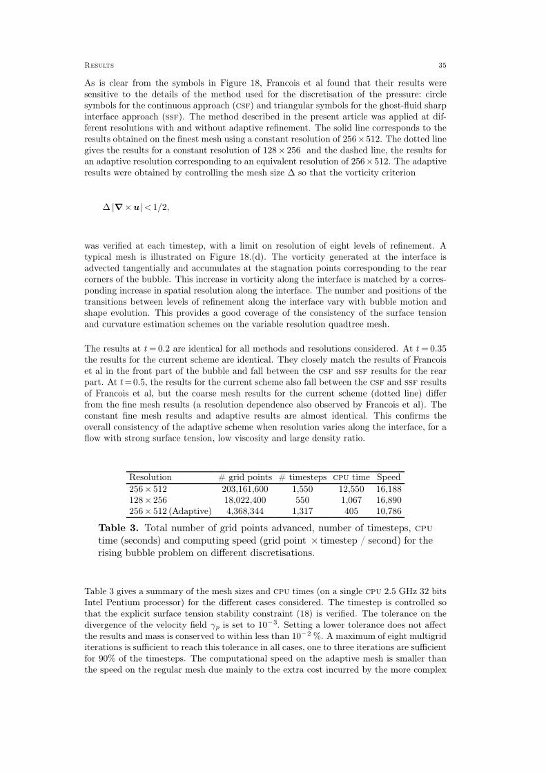
6.5 Three-dimensional capillary breakup of a liquid jet

The capillary instability of a liquid jet is a fundamental mechanism controlling the dynamicsof many important two-phase flow phenomena such as liquid/gas atomisation. It is alsowell-suited to dynamic adaptive mesh refinement as a wide range of flow scales need to beresolved, particularly around the breakup point [69, 70, 71]. Dai and Schmidt [17] used their3d adaptive unstructured tetrahedral mesh solver to study the case of the instability of aliquid cylinder with a free surface (i.e. the fluid motion of the gas phase was not resolved).Figure 19 reproduces their study (corresponding to Figure 16 of [17]) but for the case of aliquid jet surrounded by a lighter fluid.

Fig. 19. Initial stages of a capillary jet instability: k r0 = 0.628, ǫ = 0.02,La=238.34. Physical parameters correspond to a jet of water in air. The non-dimensional times are from left to right 0, 11.32 and 12.1 (breakup time). Theinterface is represented using the vof-reconstructed planar fragments in eachcell.

The computational domain is a unit box centred on the origin. Symmetry boundary con-ditions are applied for x = ± 1/2, y = − 1/2, z = − 1/2 so that only a quarter of the jet issimulated. Simple “outflow” boundary conditions are applied for y = 1/2 and z =1/2 as

∂nun = 0,

p = 0,

with n the direction normal to the boundary. The initial shape of the jet is given by radius

r(x)= r0 [1+ ǫ sin(k x)],

with r0 = 0.2, k = π and ǫ = 0.02. In order to compare with the solutions obtained fromlinear stability analysis, the velocity field is initialised as

u =∇φ with φ≡B J0(i k r) sin(k x),

36 Section 6

where the amplitude B is given by

B ≡− ǫ r0 c

i k J1(i k r0),

with c the inviscid growth rate obtained by Rayleigh [72] as

c2≡ σ

ρ r03

I1(k r0)

I0(k r0)k r0 (1− k2 r0

2).

The Laplace number La≡ σ r0/(ρ ν2) is 238.34 as in [17]. The physical parameters for thesurrounding fluid correspond to air/water density and viscosity ratios i.e. ρg/ρ = 1.2/998

and µg/µ=1.8×10−5/1.003×10−3. The density and viscosity are defined using the filteredfield c~ of equations (1) and (2).

The initial interface shape is resolved using five refinement levels. Every ten timesteps theresolution is adjusted so that for any cell containing the interface the condition ∆κmax <1/5is verified. The maximum level of refinement is set arbitrarily to ten. The timestep iscontinuously adjusted so that the stability condition (18) is verified.

Figure 20 illustrates the clean and continuous increase of resolution when approaching thebreakup point. One can also note that – despite being essentially discontinuous – the vof-reconstructed planar fragments provide a high-quality description of the interface.

Fig. 20. Details of the interface just before ((t0 − t)/Tσ = 1.5 × 10−3) andafter breakup ((t0− t)/Tσ =− 8.5× 10−3). The interface is represented usingthe vof-reconstructed planar fragments in each cell. k r0 = 0.628, ǫ = 0.02,La= 238.34.

The results are comparable to those of Dai and Schmidt although the present simulation isnot limited to a singly-connected topology. As with any vof method no special treatmentis required when breakup occurs and the simulation deals transparently with multiply

Results 37

connected interfaces (Figure 21). The maximum variation in the total mass is less than0.02%.

Fig. 21. Late stages of a capillary jet instability: k r0 = 0.628, ǫ = 0.02,La=238.34. The non-dimensional times are from left to right 12.31, 13.03 and15.36.

Weber extended the study of Rayleigh to the case of a viscous fluid [73] and obtained thefollowing equation for the growth rate of the perturbation

c2 + c 3 ν k2− σ

2 ρ r03(1− k2 r0

2) k2 r02 =0.

Figure 22 summarises the results obtained for the evolution of the initial perturbation. Twonumerical estimates of the perturbation are considered: the relative deformation associatedwith the maximum radial extent of the interface (rmax− r0)/(r0 ǫ), and the relative deform-ation associated with the minimum radial extent (r0− rmin)/(r0 ǫ). Obviously the minimumradius vanishes at the time of breakup and the associated relative deformation takes amaximum value of 1/ǫ (≈ 50). The time is made non-dimensional using Tσ≡ (ρ r0

3/σ)1/2 asreference timescale. Simulations were performed at three different Laplace numbers: 2000,238.34 and 23.834.

1

10

100

0 2 4 6 8 10 12 14 16 18

Rel

ativ

e de

form

atio

n (m

axim

um r

adiu

s)


La=2000La=238.34La=23.834RayleighWeberBreakup

1

5

10

20

50

0 2 4 6 8 10 12 14 16 18

Rel

ativ

e de

form

atio

n (m

inim

um r

adiu

s)


La=2000La=238.34La=23.834RayleighWeberBreakup

(a) (b)

Fig. 22. Evolution of the relative deformations of the interface. (a) (rmax−r0)/(r0 ǫ). (b) (r0− rmin)/(r0 ǫ).

For the maximum-radius relative deformation excellent agreement is obtained with eitherthe inviscid theory of Rayleigh (La=2000) or the viscous solution of Weber. Remarkably thegrowth rate is close to constant right up to the point of breakup. The good agreement withthe inviscid theory at high Laplace number is also indicative of the overall low numerical

38 Section 6

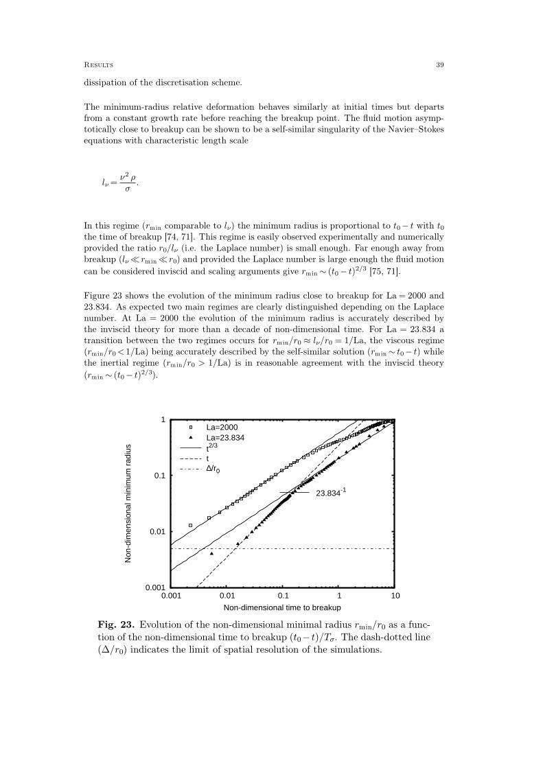
dissipation of the discretisation scheme.

The minimum-radius relative deformation behaves similarly at initial times but departsfrom a constant growth rate before reaching the breakup point. The fluid motion asymp-totically close to breakup can be shown to be a self-similar singularity of the Navier–Stokesequations with characteristic length scale

lν =ν2 ρ

σ.

In this regime (rmin comparable to lν) the minimum radius is proportional to t0− t with t0the time of breakup [74, 71]. This regime is easily observed experimentally and numericallyprovided the ratio r0/lν (i.e. the Laplace number) is small enough. Far enough away frombreakup (lν ≪ rmin≪ r0) and provided the Laplace number is large enough the fluid motion

can be considered inviscid and scaling arguments give rmin ∼ (t0− t)2/3 [75, 71].

Figure 23 shows the evolution of the minimum radius close to breakup for La = 2000 and23.834. As expected two main regimes are clearly distinguished depending on the Laplacenumber. At La = 2000 the evolution of the minimum radius is accurately described bythe inviscid theory for more than a decade of non-dimensional time. For La = 23.834 atransition between the two regimes occurs for rmin/r0 ≈ lν/r0 = 1/La, the viscous regime(rmin/r0 <1/La) being accurately described by the self-similar solution (rmin∼ t0− t) whilethe inertial regime (rmin/r0 > 1/La) is in reasonable agreement with the inviscid theory

(rmin ∼ (t0− t)2/3).

0.001

0.01

0.1

1

0.001 0.01 0.1 1 10

Non

-dim

ensi

onal

min

imum

rad

ius

Non-dimensional time to breakup

23.834-1

La=2000La=23.834t2/3

t∆/r0

Fig. 23. Evolution of the non-dimensional minimal radius rmin/r0 as a func-tion of the non-dimensional time to breakup (t0− t)/Tσ. The dash-dotted line(∆/r0) indicates the limit of spatial resolution of the simulations.

Results 39

The self-similar solution close to breakup predicts the formation of a thin liquid thread(“microthread” [76]) connecting the two regions about to separate. Although these micro-threads occur independently of the Laplace number, their characteristic length scale is lν andthey will be more easily seen at low Laplace numbers. Figure 24 illustrates the microthreadobtained numerically just before breakup for La=23.834. It looks very similar to the micro-threads observed experimentally [76, 69, 71]. The complex structure of the correspondingvelocity field is given in Figure 24.b. Interestingly the solution has two stagnation pointson the axis of symmetry (aside from the stagnation points on the symmetry planes atx=±1/2): one within the microthread (which will eventually lead to breakup) and a secondone within the “neck” region. This result is consistent with the similarity solution obtainedby Eggers [74] (see also Figure 17.b of [71]). A recirculation region within the gas phase isassociated with these two stagnation points.

(a) (b)

Fig. 24. Detail of the interface close to breakup ((t0− t)/Tσ = 1.5× 10−2) fora very viscous fluid: k r0 = 0.628, ǫ= 0.02, La= 23.834. (a) vof-reconstructedinterface. (b) Interface and streamlines in a cross-section on the axis of sym-metry.

40 Section 6

Figure 25 represents the evolution with time of the total number of leaf cells used todiscretise the problem. The step increments in the number of cells (at t ≈ 7, 11, 12, � )correspond to the addition of one additional level of refinement when the curvature of theinterface locally reaches the threshold ∆ κmax < 1/5. As expected the maximum number ofcells (≈9,000) is reached at the time of breakup. After breakup the number of cells stabilisesto about 2,500. This is larger than the initial number of cells (≈ 1,500) because the newly-created, smaller droplets require a higher resolution (rightmost Figure 21). These numberscan be compared to the number of cells which would be required with:

1. a 3d static regular Cartesian grid with an equivalent resolution (ten levels of refinement):(210)3≈ 109.

2. a 2d-axisymmetric static regular Cartesian grid: (210)2≈ 106.3. a dynamically-refined octree grid with all the cells containing the interface refined at the

same resolution ∆(t) controlled by ∆(t)max (κmax)(t)<1/5: dashed curve in Figure 25.

It is clear that orders-of-magnitude savings in computation size can be achieved when usingdynamic adaptation along the interface for this particular problem. Option 3 above whichhas been used in a number of recent studies [28, 30, 8, 36, 31, 9, 38, 64, 33, 39] is simpleto implement within a vof framework but does not make full use of adaptivity. The totalcpu time (≈ 6,000 timesteps) for the simulation of Figures 19–21, 25 is about three hourson a 2.5 GHz 32 bits Intel Pentium processor.

1000

10000

100000

1e+06

1e+07

0 2 4 6 8 10 12 14 16 18

Num

ber

of le

af c

ells


AdaptiveOption 3 (estimated)

Fig. 25. Evolution of the total number of leaf cells required to discretisethe jet while verifying the criterion ∆ κmax < 1/5. Maximum of ten levels ofrefinement. k r0 = 0.628, ǫ = 0.02, La= 238.34.

Results 41

Finally the three-dimensional results are cross-validated against axisymmetric results bothwith and without variable resolution along the interface. The axisymmetric results areobtained using a cylindrical-coordinates version of the code with k r0 = 0.628, ǫ = 0.02,La= 2000. Two types of refinement are considered:

a) A dynamically refined quadtree grid with all the cells containing the interface refined atthe same resolution ∆(t) controlled by ∆(t)max (κmax(s))(t) < 1/5, with s the surfacecoordinate on the interface (equivalent to option 3 above).

b) A dynamically refined quadtree grid with variable resolution along the interface ∆(s, t)controlled by ∆(s, t) κmax(s, t) < 1/5 (corresponding to the 3D simulation).

0

0.1

0.2

0.3

0.4

0.5

-0.4 -0.2 0 0.2 0.4

Axi ∆(s,t)Axi ∆(t)

3D ∆(s,t)

0

0.1

0.2

0.3

0.4

0.5

-0.4 -0.2 0 0.2 0.4


3D ∆(s,t)

(a) (b)

0

0.1

0.2

0.3

0.4

0.5

-0.4 -0.2 0 0.2 0.4


3D ∆(s,t)

0

0.005

0.01

0.015

0.02

0.025

0.08 0.09 0.1 0.11 0.12 0.13


3D ∆(s,t)

(c) (d)

Fig. 26. Comparison of axisymmetric and three-dimensional interface pro-files. k r0 = 0.628, ǫ = 0.02, La= 2000. (a) t/Tσ = 11.51. (b) t/Tσ = 11.61. (c)t/Tσ = 11.79. (d) Detail corresponding to the rectangular area in (b).

Figure 26 summarises the results for these three cases: before breakup (a), close to breakup(b) and (d), and some time after breakup (c). The three-dimensional profile is obtainedas a cross-section on the axis of symmetry of the 3D vof-reconstructed surface. The 3Dsolution is almost exactly axisymmetric and the choice of cross-section plane does not affectthe results. The general agreement between the three solutions is excellent. Before breakupthe axisymmetric results are almost identical. The small discrepancy between the 3D andaxisymmetric results could be due to the fact that the second principal radius of curvature(in the plane perpendicular to the plane of axisymmetry) is computed completely differentlyin the axisymmetric and 3D cases. Breakup occurs slightly later for the axisymmetric ∆(s,

t) case which explains the somewhat larger discrepancy between the axisymmetric resultsat later times (Figure 26.c).

Table 4 gives the corresponding mesh sizes, number of timesteps and speeds (per gridpoint and timestep). The numbers for the 3d ∆(t) case are estimated assuming the samecomputing speed as in the 3d ∆(s, t) case. The axisymmetric ∆(s, t) and 3d cases save

42 Section 6

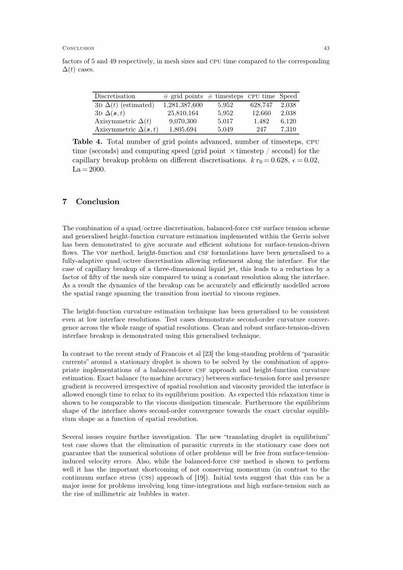
factors of 5 and 49 respectively, in mesh sizes and cpu time compared to the corresponding∆(t) cases.

Discretisation # grid points # timesteps cpu time Speed

3d ∆(t) (estimated) 1,281,387,600 5,952 628,747 2,0383d ∆(s, t) 25,810,164 5,952 12,660 2,038Axisymmetric ∆(t) 9,070,300 5,017 1,482 6,120Axisymmetric ∆(s, t) 1,805,694 5,049 247 7,310

Table 4. Total number of grid points advanced, number of timesteps, cputime (seconds) and computing speed (grid point × timestep / second) for thecapillary breakup problem on different discretisations. k r0 = 0.628, ǫ = 0.02,La= 2000.

7 Conclusion

The combination of a quad/octree discretisation, balanced-force csf surface tension schemeand generalised height-function curvature estimation implemented within the Gerris solverhas been demonstrated to give accurate and efficient solutions for surface-tension-drivenflows. The vof method, height-function and csf formulations have been generalised to afully-adaptive quad/octree discretisation allowing refinement along the interface. For thecase of capillary breakup of a three-dimensional liquid jet, this leads to a reduction by afactor of fifty of the mesh size compared to using a constant resolution along the interface.As a result the dynamics of the breakup can be accurately and efficiently modelled acrossthe spatial range spanning the transition from inertial to viscous regimes.

The height-function curvature estimation technique has been generalised to be consistenteven at low interface resolutions. Test cases demonstrate second-order curvature conver-gence across the whole range of spatial resolutions. Clean and robust surface-tension-driveninterface breakup is demonstrated using this generalised technique.

In contrast to the recent study of Francois et al [23] the long-standing problem of “parasiticcurrents” around a stationary droplet is shown to be solved by the combination of appro-priate implementations of a balanced-force csf approach and height-function curvatureestimation. Exact balance (to machine accuracy) between surface-tension force and pressuregradient is recovered irrespective of spatial resolution and viscosity provided the interface isallowed enough time to relax to its equilibrium position. As expected this relaxation time isshown to be comparable to the viscous dissipation timescale. Furthermore the equilibriumshape of the interface shows second-order convergence towards the exact circular equilib-rium shape as a function of spatial resolution.

Several issues require further investigation. The new “translating droplet in equilibrium”test case shows that the elimination of parasitic currents in the stationary case does notguarantee that the numerical solutions of other problems will be free from surface-tension-induced velocity errors. Also, while the balanced-force csf method is shown to performwell it has the important shortcoming of not conserving momentum (in contrast to thecontinuum surface stress (css) approach of [19]). Initial tests suggest that this can be amajor issue for problems involving long time-integrations and high surface-tension such asthe rise of millimetric air bubbles in water.

Conclusion 43

Finally, I hope that providing the full implementation of the method as part of the freely-modifiable open source software Gerris [44] will encourage other people to tackle theseissues.

Acknowledgements

This work was funded by the New Zealand Foundation for Research, Science and Technologyunder contract no. CO1X0204.

References

[1] C. Hirt, B. Nichols, Volume of fluid method for the dynamics of free boundaries, Journal of Computa-

tional Physics 39 (1) (1981) 201–225.

[2] J. Li, Calcul d’interface affine par morceaux, Comptes rendus de l’Académie des sciences. Série II,

Mécanique, physique, chimie, astronomie 320 (8) (1995) 391–396.

[3] W. Rider, D. Kothe, Reconstructing volume tracking, Journal of Computational Physics 141 (2) (1998)

112–152.

[4] R. Scardovelli, S. Zaleski, Direct numerical simulation of free-surface and interfacial flow, Annual

Review of Fluid Mechanics 31 (1) (1999) 567–603.

[5] M. Sussman, P. Smereka, S. Osher, A level set approach for computing solutions to incompressible two-

phase flow, Journal of Computational Physics 114 (1) (1994) 146–159.

[6] M. Sussman, A. Almgren, J. Bell, P. Colella, L. Howell, M. Welcome, An adaptive level set approach

for incompressible two-phase flows, Journal of Computational Physics 148 (1) (1999) 81–124.

[7] V. Sochnikov, S. Efrima, Level set calculations of the evolution of boundaries on a dynamically adaptive

grid, International Journal for Numerical Methods in Engineering 56 (2003) 1913–1929.

[8] H. Kohno, T. Tanahashi, Numerical analysis of moving interfaces using a level set method coupled with

adaptive mesh refinement, International Journal for Numerical Methods in Fluids 45 (2004) 921–944.

[9] X. Zheng, J. Lowengrub, A. Anderson, V. Cristini, Adaptive unstructured volume remeshing–II: Applic-

ation to two-and three-dimensional level-set simulations of multiphase flow, Journal of Computational

Physics 208 (2) (2005) 626–650.

[10] H. Liu, S. Krishnan, S. Marella, H. Udaykumar, Sharp interface cartesian grid method ii: A technique

for simulating droplet interactions with surfaces of arbitrary shape, Journal of Computational Physics

210 (1) (2005) 32 – 54.

[11] E. Marchandise, J.-F. Remacle, A stabilized finite element method using a discontinuous level set

approach for solving two phase incompressible flows, Journal of Computational Physics 219 (2) (2006)

780 – 800.

[12] E. Marchandise, P. Geuzaine, N. Chevaugeon, J.-F. Remacle, A stabilized finite element method using

a discontinuous level set approach for the computation of bubble dynamics, Journal of Computational

Physics 225 (1) (2007) 949 – 974.

[13] O. Desjardins, V. Moureau, H. Pitsch, An accurate conservative level set/ghost fluid method for

simulating turbulent atomization, Journal of Computational Physics 227 (18) (2008) 8395 – 8416.

[14] D. Fyfe, E. Oran, M. Fritts, Surface tension and viscosity with Lagrangian hydrodynamics on a

triangular mesh, Journal of Computational Physics 76 (2) (1988) 349–384.

[15] S. Popinet, S. Zaleski, A front-tracking algorithm for accurate representation of surface tension,

International Journal for Numerical Methods in Fluids 30 (6) (1999) 775–793.

[16] S. Shin, S. Abdel-Khalik, V. Daru, D. Juric, Accurate representation of surface tension using the level

contour reconstruction method, Journal of Computational Physics 203 (2) (2005) 493–516.

[17] M. Dai, D. Schmidt, Adaptive tetrahedral meshing in free-surface flow, Journal of Computational

Physics 208 (1) (2005) 228–252.

44 Section

[18] B. Lafaurie, C. Nardone, R. Scardovelli, S. Zaleski, G. Zanetti, Modelling merging and fragmentation

in multiphase flows with SURFER, Journal of Computational Physics 113 (1) (1994) 134–147.

[19] D. Gueyffier, A. Nadim, J. Li, R. Scardovelli, S. Zaleski, Volume of fluid interface tracking with

smoothed surface stress methods for three-dimensional flows, Journal of Computational Physics 152

(1998) 423–456.

[20] M. Kang, R. Fedkiw, X. Liu, A boundary condition capturing method for multiphase incompressible

flow, Journal of Scientific Computing 15 (3) (2000) 323–360.

[21] Y. Renardy, M. Renardy, PROST - A parabolic reconstruction of surface tension for the volume-of-

fluid method, Journal of Computational Physics 183 (2) (2002) 400–421.

[22] D. Harvie, M. Davidson, M. Rudman, An analysis of parasitic current generation in volume of fluid

simulations, Applied Mathematical Modelling 30 (10) (2006) 1056–1066.

[23] M. Francois, S. Cummins, E. Dendy, D. Kothe, J. Sicilian, M. Williams, A balanced-force algorithm

for continuous and sharp interfacial surface tension models within a volume tracking framework, Journal

of Computational Physics 213 (1) (2006) 141–173.

[24] I. Ginzburg, G. Wittum, Two-phase flows on interface refined grids modeled with VOF, staggered

finite volumes, and spline interpolants, Journal of Computational Physics 166 (2) (2001) 302–335.

[25] S. Cummins, M. Francois, D. Kothe, Estimating curvature from volume fractions, Computers and

Structures 83 (6-7) (2005) 425–434.

[26] M. Sussman, M. Ohta, Improvements for calculating two-phase bubble and drop motion using an

adaptive sharp interface method, Fluid Dyn. Mater. Proc. 3 (1) (2007) 21–36.

[27] A. Almgren, J. Bell, P. Colella, L. Howell, M. Welcome, A conservative adaptive projection method for

the variable density incompressible Navier–Stokes equations, Journal of Computational Physics 142 (1)

(1998) 1–46.

[28] J. Jeong, D. Yang, Finite element analysis of transient fluid flow with free surface using VOF (volume-

of-fluid) method and adaptive grid, International Journal for Numerical Methods in Fluids 26 (10) (1998)

1127–1154.

[29] M. Sussman, A parallelized, adaptive algorithm for multiphase flows in general geometries, Computers

& Structures 83 (6-7) (2005) 435 – 444.

[30] D. Greaves, A quadtree adaptive method for simulating fluid flows with moving interfaces, Journal

of Computational Physics 194 (1) (2004) 35–56.

[31] A. Theodorakakos, G. Bergeles, Simulation of sharp gas–liquid interface using VOF method and

adaptive grid local refinement around the interface, International Journal for Numerical Methods in

Fluids 45 (4) (2004) 421–439.

[32] F. Losasso, R. Fedkiw, S. Osher, Spatially adaptive techniques for level set methods and incompressible

flow, Computers and Fluids 35 (2006) 457–462.

[33] C. Min, F. Gibou, A second order accurate level set method on non-graded adaptive Cartesian grids,

Journal of Computational Physics 225 (1) (2007) 300–321.

[34] G. Compère, E. Marchandise, J.-F. Remacle, Transient adaptivity applied to two-phase incompressible

flows, Journal of Computational Physics 227 (3) (2008) 1923 – 1942.

[35] S. Popinet, Gerris: a tree-based adaptive solver for the incompressible Euler equations in complex

geometries, Journal of Computational Physics 190 (2) (2003) 572–600.

[36] J. Wang, A. Borthwick, R. Taylor, Finite-volume-type VOF method on dynamically adaptive quadtree

grids, International Journal for Numerical Methods in Fluids 45 (5) (2004) 485–508.

[37] F. Losasso, F. Gibou, R. Fedkiw, Simulating water and smoke with an octree data structure, ACM

Transactions on Graphics (TOG) 23 (3) (2004) 457–462.

[38] D. Greaves, Simulation of viscous water column collapse using adapting hierarchical grids, Interna-

tional Journal for Numerical Methods in Fluids 50 (6) (2006) 693–711.

[39] N. Nikolopoulos, A. Theodorakakos, G. Bergeles, Three-dimensional numerical investigation of a

droplet impinging normally onto a wall film, Journal of Computational Physics 225 (1) (2007) 322–341.

[40] M. Herrmann, A balanced force refined level set grid method for two-phase flows on unstructured flow

solver grids, Journal of Computational Physics 227 (4) (2008) 2674–2706.

[41] M. Malik, E. Sheung-Chi Fan, M. Bussmann, Adaptive VOF with curvature-based refinement, Inter-

national Journal for Numerical Methods in Fluids 55 (7) (2007) 693–712.

[42] M. Rudman, Volume-tracking methods for interfacial flows calculations, International Journal for

Numerical Methods in Fluids 24 (7) (1997) 671–691.

References 45

[43] M. Sussman, K. Smith, M. Hussaini, M. Ohta, R. Zhi-Wei, A sharp interface method for incompressible

two-phase flows, Journal of Computational Physics 221 (2) (2007) 469–505.

[44] S. Popinet, The Gerris Flow Solver, http://gfs.sf.net (2007).

[45] S. Popinet, Gerris Test Suite, http://gfs.sourceforge.net/tests/tests/index.html (2007).

[46] A. Chorin, On the convergence of discrete approximations to the Navier–Stokes equations, Mathem-

atics of Computation 23 (106) (1969) 341–353.

[47] R. Alcouffe, A. Brandt, J. Dendy Jr, J. Painter, The multi-grid method for the diffusion equation with

strongly discontinuous coefficients, SIAM Journal on Scientific and Statistical Computing 2 (1981) 430.

[48] O. Tatebe, N. Melson, T. Manteuffel, S. McCormick, The multigrid preconditioned conjugate gradient

method, in: Sixth Copper Mountain Conference on Multigrid Methods, NASA, 1993, pp. 621–634.

[49] T. Chan, W. Wan, Robust multigrid methods for nonsmooth coefficient elliptic linear systems, Journal

of Computational and Applied Mathematics 123 (1-2) (2000) 323–352.

[50] J. Bell, P. Colella, H. Glaz, A second-order projection method for the incompressible Navier–Stokes

equations, Journal of Computational Physics 85 (1989) 257–283.

[51] A. Almgren, J. Bell, W. Crutchfield, Approximate projection methods: part I. inviscid analysis, SIAM

Journal on Scientific Computing 22 (4) (2000) 1139–1159.

[52] R. Scardovelli, S. Zaleski, Analytical relations connecting linear interfaces and volume fractions in

rectangular grids, Journal of Computational Physics 164 (1) (2000) 228–237.

[53] R. Scardovelli, S. Zaleski, Interface reconstruction with least-square fit and split eulerian–lagrangian

advection, International Journal for Numerical Methods in Fluids 41 (2003) 251–274.

[54] E. Aulisa, S. Manservisi, R. Scardovelli, S. Zaleski, Interface reconstruction with least-squares fit

and split advection in three-dimensional Cartesian geometry, Journal of Computational Physics 225 (2)

(2007) 2301–2319.

[55] R. DeBar, Fundamentals of the KRAKEN code, Tech. rep., UCID-17366, California Univ., Livermore

(USA). Lawrence Livermore Lab. (1974).

[56] D. Lörstad, L. Fuchs, High-order surface tension VOF-model for 3D bubble flows with high density

ratio, Journal of Computational Physics 200 (1) (2004) 153–176.

[57] S. Zalesak, Fully multidimensional flux-corrected transport algorithms for fluids, Journal of Compu-

tational Physics 31 (3) (1979) 335–362.

[58] O. Ubbink, R. Issa, A method for capturing sharp fluid interfaces on arbitrary meshes, Journal of

Computational Physics 153 (1) (1999) 26–50.

[59] W. Noh, P. Woodward, SLIC/simple line interface calculation, International Conference on Numerical

Methods in Fluid Dynamics, 5th, Enschede, Netherlands, June 28-July 2, 1976, .

[60] E. Aulisa, S. Manservisi, R. Scardovelli, S. Zaleski, A geometrical area-preserving volume-of-fluid

method, Journal of Computational Physics 192 (2003) 355–364.

[61] M. Sussman, A second order coupled level set and volume-of-fluid method for computing growth and

collapse of vapor bubbles, Journal of Computational Physics 187 (1) (2003) 110 – 136.

[62] J. Brackbill, D. Kothe, C. Zemach, A continuum method for modeling surface tension, Journal of

Computational Physics 100 (2) (1992) 335–354.

[63] M. Sussman, E. Puckett, A coupled level set and volume of fluid method for computing 3D and

axisymmetric incompressible two-phase flows, Journal of Computational Physics 162 (2) (2000) 301–337.

[64] X. Yang, A. James, J. Lowengrub, X. Zheng, V. Cristini, An adaptive coupled level-set/volume-of-

fluid interface capturing method for unstructured triangular grids, Journal of Computational Physics

217 (2) (2006) 364–394.

[65] M. Torrey, L. Cloutman, R. Mjolsness, C. Hirt, NASA-VOF2D: a computer program for incompress-

ible flows with free surfaces, Tech. rep., Los Alamos National Laboratory (1985).

[66] D. Gerlach, G. Tomar, G. Biswas, F. Durst, Comparison of volume-of-fluid methods for surface

tension-dominant two-phase flows, International Journal of Heat and Mass Transfer 49 (3-4) (2006) 740–

754.

[67] H. Lamb, Hydrodynamics, Cambridge University Press, 1971.

[68] A. Prosperetti, Motion of two superposed viscous fluids, Physics of Fluids 24 (1981) 1217.

[69] X. Shi, M. Brenner, S. Nagel, A cascade of structure in a drop falling from a faucet, Science 265 (5169)

(1994) 219–222.

46 Section

[70] M. Brenner, J. Eggers, K. Joseph, S. Nagel, X. D. Shi, Breakdown of scaling in droplet fission at high

Reynolds number, Physics of Fluids 9 (6) (1997) 1573–1590.

[71] J. Eggers, Nonlinear dynamics and breakup of free-surface flows, Reviews of Modern Physics 69 (3)

(1997) 865–930.

[72] L. Rayleigh, On the instability of a cylinder of viscous liquid under capillary force, Philosophical

Magazine 34 (207) (1892) 145–154.

[73] C. Weber, Disintegration of liquid jets, Zeitschrift für Angewandte Mathematik und Mechanik 11 (2)

(1931) 136–159.

[74] J. Eggers, Universal pinching of 3D axisymmetric free-surface flow, Physical Review Letters 71 (21)

(1993) 3458–3460.

[75] D. Peregrine, G. Shoker, A. Symon, The bifurcation of liquid bridges, Journal of Fluid Mechanics 212

(1990) 25–39.

[76] T. Kowalewski, On the separation of droplets from a liquid jet, Fluid Dynamics Research 17 (1996)

121–145.

References 47

An accurate adaptive solver for surface-tension …gfs.sourceforge.net/papers/tension.pdfAn accurate...

Documents

Transcript of An accurate adaptive solver for surface-tension …gfs.sourceforge.net/papers/tension.pdfAn accurate...