AN ABSTRACT OF THESIS OF Sam Goodrich for the degree of

AN ABSTRACT OF THESIS OF

Sam Goodrich for the degree of Master of Science in Nuclear Engineering presented on

June 21, 2013.

Title: Design, Fabrication, and Characterization of the Laser-Imaged Natural Circulation

(LINC) Facility

Abstract approved:____________________________________________________

Wade R. Marcum

Currently there is a great amount of interest in the phenomena of natural circulation as a

cooling mechanism for normal operation as well as emergency conditions in nuclear

reactors and spent fuel pools. In order to better understand this phenomena for the specific

geometry of vertical, heated rods in water, an experimental facility was designed and

constructed at Oregon State University. This facility, named the Laser-Imaged Natural

Circulation (LINC) facility, consists of a water tank capped with a custom cooling plate

through which two heated rods pass into the tank. The LINC facility enables flow patterns

in the channel between the heated rods to be imaged and quantified using particle image

velocimetry (PIV).

This paper presents the reasoning and theory behind the design of the LINC facility, as

well as a characterization of the thermodynamics, boundary layer thickness and velocity

profile progression of the system. The thermodynamic analysis consists of bulk equilibrium

temperatures and heat removal rates for 3 cases where the two heater rods have equal power

levels (dubbed “symmetrical heating”). The boundary layer thickness analysis consists of

a test matrix of 5 test cases including symmetrical and asymmetrical heating in which the

thickness of the boundary layer is measured using the velocity field between the heater

rods. The velocity profile analysis centered on an effective vertical length of 100 mm along

the entrance region between the two rods at one symmetrical rod power. In addition to

these experiments, additional synthesis of data regarding the dependence of the Nusselt

number on the Rayleigh number along with temperature profile of the boundary layer were

collected and presented.

© Copyright by Sam Goodrich

June 21, 2013

All Rights Reserved

Design, Fabrication, and Characterization of the Laser-Imaged Natural Circulation

(LINC) Facility

by

Sam Goodrich

A THESIS

Submitted to

Oregon State University

in partial fulfillment of

the requirements for the

degree of

Master of Science

Presented June 21, 2013

Commencement June 2014

Master of Science thesis of Sam Goodrich presented on June, 21 2013.

APPROVED:

_____________________________________________________________________

Major Professor, representing Nuclear Engineering

_____________________________________________________________________

Head of the Department of Nuclear Engineering and Radiation Health Physics

_____________________________________________________________________

Dean of the Graduate School

I understand that my thesis will become part of the permanent collection of Oregon State

University libraries. My signature below authorizes release of my thesis to any reader upon

request.

_____________________________________________________________________

Sam Goodrich, Author

ACKNOWLEDGEMENTS

I would like to thank my friends, family and colleagues. Their friendship and collaboration

have made graduate school an enjoyable experience.

I would especially like to thank my wonderful wife Jess. She is the most supportive, kind

and understanding person I have ever known. I would like to thank her and my boys, James

and David, for being understanding when I needed to work extra hours.

I would like to thank my advisor, Dr. Marcum for all of the help and support he has

provided in this work and for always making time to help out. Working with Dr. Marcum

has helped me learn to be a better student, professional, and scientist.

Finally, I would like to thank my parents for never considering it a possibility that I might

not be able to achieve my ambitions.

TABLE OF CONTENTS

Section Page

1 Introduction ................................................................................................................... 1

1.1 Objectives .............................................................................................................. 2

1.2 Document Overview ............................................................................................. 3

2 Survey of Literature ...................................................................................................... 5

2.1 Natural Circulation Phenomena ............................................................................ 5

2.2 Flow Visualization Using Particle Image Velocimetry ....................................... 10

3 Theory ......................................................................................................................... 13

3.1 Material Properties .............................................................................................. 13

3.1.1 Properties of water ......................................................................................... 13

3.1.2 Properties of Copper ...................................................................................... 14

3.1.3 Other Materials .............................................................................................. 15

3.1.3.1 Incoloy 800 ............................................................................................ 15

3.1.3.2 Magnesium Oxide (MgO) ...................................................................... 15

3.2 Derived Parameters ............................................................................................. 16

3.2.1 Volumetric Thermal expansion coefficient (β) ............................................. 16

3.2.2 Kinematic Viscosity ...................................................................................... 16

3.3 Dimensional Analysis ......................................................................................... 17

3.3.1 Biot Number .................................................................................................. 21

3.3.2 Prandtl Number ............................................................................................. 21

3.3.3 Grashof Number ............................................................................................ 22

3.3.4 Rayleigh Number .......................................................................................... 22

3.4 Natural Circulation Loop .................................................................................... 23

3.4.1 Heat transfer in Cooling Plate ....................................................................... 25

3.4.2 Heat transfer from heater rods ....................................................................... 28

3.5 Natural Circulation & Boundary Layer Development ........................................ 32

3.6 Particle Image Velocimetry ................................................................................. 33

TABLE OF CONTENTS (Continued)

Section Page

4 Experimental Facility .................................................................................................. 38

4.1 Design Bases ....................................................................................................... 40

4.1.1 Tank design ................................................................................................... 40

4.1.2 Cooling Plate Design ..................................................................................... 42

4.2 Experimental Equipment and Specifications ...................................................... 46

4.2.1 Heaters & Cooling ......................................................................................... 46

4.2.2 Instrumentation .............................................................................................. 48

4.2.3 PIV System .................................................................................................... 48

4.3 Procedure and Set-up for Characterization Experiments .................................... 49

4.3.1 Thermal Equilibrium Analysis ...................................................................... 49

4.3.2 Boundary Layer Thickness Analysis ............................................................. 51

4.3.3 Velocity Profile Analysis .............................................................................. 54

5 Results and Discussion ............................................................................................... 56

5.1 Energy Balance Characterization ........................................................................ 56

5.2 Boundary Layer Characterization ....................................................................... 62

5.3 Velocity Profile Characterization ........................................................................ 70

5.4 The Nusselt Number and the Transverse Curvature Effect ................................. 77

5.5 Temperature Profiles ........................................................................................... 79

6 Conclusion .................................................................................................................. 83

6.1 Observations ........................................................................................................ 83

6.2 Relevance of Work .............................................................................................. 84

6.3 Experimental Limitations .................................................................................... 85

6.4 Future Work ........................................................................................................ 86

7 Works Cited ................................................................................................................ 88

8 Nomenclature .............................................................................................................. 97

9 Appendix A: Uncertainty Analysis ........................................................................... 101

10 Appendix B: Experimental Facility Drawings .......................................................... 106

LIST OF FIGURES

Figure Page

Figure 3.1 Boundary layer sketch showing coordinate conventions ................................ 17

Figure 3.2 Illustration of LINC facility circulation loops ................................................. 24

Figure 3.3 Illustration of heat transfer mechanisms in primary and secondary loops ...... 24

Figure 3.4 Illustration of cross-section of heater rod ........................................................ 31

Figure 3.5 Summary of PIV analysis process using images from the LINC facility ........ 34

Figure 3.6 Cross correlation map acquired from LINC facility data ................................ 36

Figure 4.1 Overview of LINC facility .............................................................................. 39

Figure 4.2 Rendering of LINC facility close up ............................................................... 40

Figure 4.3 Tank sketch with dimensions .......................................................................... 41

Figure 4.4 Detail of cross section of cooling plate with labels ......................................... 43

Figure 4.5 Rendering of side A of cooling plate ............................................................... 44

Figure 4.6 Rendering of side B of cooling plate ............................................................... 44

Figure 4.7 Cooling configuration of cooling plate............................................................ 45

Figure 4.8 Cross section view of heater rod design. Image courtesy of Bucan ................ 47

Figure 5.1 Temperature equilibrium plot for 200W rod power ........................................ 57

Figure 5.2 Power equilibrium plot for 200W rod power .................................................. 57





Figure 5.7 Equilibrium temperature comparison summary .............................................. 60

Figure 5.8 Equilibrium power comparison summary ....................................................... 60

Figure 5.9 Surface/contour plot of V with accurate aspect ratio test case 4 ..................... 63

Figure 5.10 Surface/contour plot of V for full profile test case 4 ..................................... 64

Figure 5.11 Boundary layer comparison Case 1 ............................................................... 66



https://d.docs.live.net/7b7172156350a718/Masters%20Work/Goodrich_Thesis_Rev3.docx#_Toc360544964

LIST OF FIGURES (Continued)

Figure Page



Figure 5.16 Colorized surface plot of V for test case 5 .................................................... 68

Figure 5.17 Surface plot of velocity profile for 200W power .......................................... 71

Figure 5.18 Velocity profile development in absolute units a 200W ............................... 72

Figure 5.19 Normalized velocity profile development at 200W ...................................... 73

Figure 5.20 Velocity profile from Eckert ......................................................................... 73

Figure 5.21 Velocity Profile at Ra=1.5E6 (13.22mm from leading edge) ....................... 75

Figure 5.22 Velocity Profile at Ra=5.4E7 (43.1mm from leading edge) ......................... 76

Figure 5.23 Velocity Profile at Ra=5E8 (90.75mm from leading edge) .......................... 76

Figure 5.24 Nu vs. Ra for current work compared with prior work ................................. 78

Figure 5.25 Temperature profile for 200W symmetrical heating case ............................. 80

Figure 5.26 Temperature Profile for 300W symmetrical heating case ............................. 80

Figure 5.27 Temperature profile for 400W symmetrical heating case ............................. 81

Figure 10.1 Rendering of LINC facility ......................................................................... 106

Figure 10.2 Rear view rendering of LINC facility ......................................................... 107

Figure 10.3 Cooling Plate Side A Top View Detail ....................................................... 108

Figure 10.4 Cooling Plate Side A Bottom View Detail .................................................. 108

Figure 10.5 Cooling Plate Side B Top View Detail........................................................ 108

Figure 10.6 Heater Rod Clamp Side 1 Detail ................................................................. 108

Figure 10.7 Heater Rod Clamp Side 2 Detail ................................................................. 108

Figure 10.8 Parts List ...................................................................................................... 108







LIST OF TABLES

Table Page

Table 4.1 Boundary Layer Experimental Test Matrix ...................................................... 54

Table 9.1 Tabulated Error for Cooling Calculation Components ................................... 102

Table 9.2 Equilibrium Plate Power Removal Uncertainty .............................................. 102

Table 9.3 Tabulated component error for surface temperature calculation .................... 103

Table 9.4 Tabulated component error for Ra calculation ............................................... 103

Table 9.5 Uncertainty in Ra for 4 thermal equilibrium cases ......................................... 104

Table 9.6 Tabulated error for Nu calculation.................................................................. 104

Table 9.7 Uncertainty in Nu for 4 thermal equilibrium cases......................................... 104

Table 9.8 Standard deviation of V used in velocity profile analysis (mm/s) .................. 105

Design, Fabrication, and Characterization of the Laser-Imaged Natural Circulation

(LINC) Facility

1 INTRODUCTION

There is currently significant interest in the energy vertical centered on small, modular

reactors (SMRs) [1]. The International Atomic Energy Association (IAEA) classifies any

commercial nuclear power reactor with a design power output of 300 MW electric or less

as a small modular reactor [2]. This reactor concept enables manufacturing of reactor

components such as the pressure vessel at a central location with flexibility to distribute a

unit to remote locations. Furthermore, several companies have adopted the concept of

ganging multiple units together to accommodate economy of scale. One unique design

feature of many SMRs is a passively cooled core which makes several design-basis

accidents associated with Generation II, Generation III and Generation III+ reactors

obsolete [3], [4]. The passive cooling in the core is achieved by natural convection, also

known as natural circulation. Fuel rods locally heat water (used as a coolant and moderator

in light water SMRs), which reduces its density and generates buoyancy-driven flow

upward to a heat exchanger. This heat is removed and the coolant then becomes more

dense, flowing downward in the closed loop to be heated again. In this way SMRs maintain

passive cooling in their core as long as the buoyancy forces created by the fuel and heat

exchanger exceed resistive forces in the loop. While much is known about the principles

governing natural convection, many questions remain [4]. In order to begin to answer some

of these questions, the Laser-Imaged Natural Circulation (LINC) facility was designed and

constructed at Oregon State University (OSU). The facility consists of a primary and

secondary loop where natural convection occurs in the primary loop via heater rods and a

cooling plate. In this study, the design-basis calculations are presented to support the

decisions behind the design of the facility. In addition, experiments were conducted using

the facility to evaluate the accuracy of the design-basis calculations. These experiments

2

involved a study of (1) the thermodynamic behavior of the system, (2) the determination

of the boundary layer thickness at a series of heating conditions, and (3) an analysis of the

velocity profile development at a single heating condition. In addition, a preliminary

evaluation of the Nusselt (Nu) number of the heater rods as a function of the Rayleigh (Ra)

number was performed as well as a temperature profile measurement adjacent to the rods.

The results of this characterization study are presented and discussed herein.

1.1 Objectives

The objectives of this work can be divided into two categories: long-term and short-term.

The long-term objective is to add to the body of knowledge regarding natural circulation

adjacent to vertical, heated cylinders by gathering experimental data about said phenomena

within a body of water. The short-term objective, in support of the long-term objective, is

to design, construct, and characterize the LINC facility. In order to fulfil the short-term

objective, specific tasks were performed:

An experimental apparatus was designed to create small-scale natural circulation

conditions in water adjacent to a heated vertical surface, the velocity of which

could be measured and quantified using particle image velocimetry (PIV). This

facility is called the LINC facility.

The LINC facility was fabricated and constructed at OSU and all instrumentation

and auxiliary equipment was installed.

A characterization study was performed using the LINC facility to collect data to

compare against design basis calculations. This characterization was done in three

primary parts:

o The facility was used to measure the thermal equilibrium values of bulk

temperature, heat removed by the cooling plate and a rough temperature

profile. This data was compared to the design basis model.

3

o The boundary layer thickness was measured for a series of five symmetrical

and asymmetrical heating conditions between the heater rods and compared

to estimates provided in literature.

o The velocity profile development was measured for a symmetrical heating

case of 200W from the leading edge to 100 mm upstream. This velocity

profile progression was compared with previous work.

1.2 Document Overview

This thesis consists of the following outlined content.

Chapter 1: Introduction – An introduction to the need for basic natural circulation

research, including a list of objectives and tasks to address this need.

Chapter 2: Survey of Literature – Background information summarizing prior work in

the fields of natural circulation and particle image velocimetry.

Chapter 3: Theory – A detailed treatment of the theory, equations and correlations used

to design the LINC facility and characterize it. Included is a summary of physical properties

used, the correlations used to model the energy balance of the system, an introduction to

natural circulation and boundary layer development, and a primer on particle image

velocimetry.

Chapter 4: Experimental Facility – A detailed description of the experimental facility

and reasoning behind the design. Also, an explanation of the procedures used for both the

experimental and modeling work to address the characterization objectives.

4

Chapter 5: Results and Discussion – A presentation of the results of the experiments

outlined in the objectives, a comparison to the design basis calculations, and a discussion

of the performance of the facility.

Chapter 6: Conclusion – Conclusions drawn from the results of the work performed and

a brief discussion of limitations and future work.

At the end of the document the reader will find references, a table of nomenclature and

appendices. Appendix A contains an uncertainty analysis of the experimental data and

Appendix B contains detailed drawings of the experimental facility.

5

2 SURVEY OF LITERATURE

Significant scientific work has been focused on the area of natural circulation for both

closed and open systems. Additionally, recently developed experimental techniques such

as PIV have been applied toward the characterization of complex fluid flow fields, like

those in natural circulation driven conditions. This chapter addresses a compressed

summary of relevant work in the area of natural circulation phenomena in an attempt to

discover what has been done before and also what needs to be done to progress the science.

In addition, a summary of the development and use of PIV as a fluid flow field imaging

technique is presented in order to provide context regarding strengths and limitations when

applying the technique to natural circulation.

2.1 Natural Circulation Phenomena

Examples of natural circulation abound in nature and as such, have likely been studied for

centuries. One early pioneer in furthering understanding of natural circulation was Lorenz

[5]. In Lorenz’s analytical study, he assumed that the only relevant velocity in the fluid

flow boundary was that parallel to a heated vertical plate and that temperature in the fluid

was a function of distance from the plate only. While the efforts of Lorenz (1881) were a

significant beginning to analytical understanding of natural convection, some of the first

published experimental results on the topic were those by Lorenz (1934) [6] and Colburn

and Hougen [7] where Lorenz measured the heat loss from a 12 cm tall plate that was

immersed in oil while Colburn and Hougen measured the heat loss from a vertical cylinder.

Elenbaas [8] addressed a need for an analysis of a more complex system than a single

vertical plate or cylinder in 1942. He examined natural circulation of air between pairs of

isothermal plates ranging in size from 5.95 x 5.95 cm, 12 x 12 cm and 24 x 24 cm. The

thickness of the plates were 6mm, 6mm and 10mm, respectively. The ambient temperature

was varied from 10°C to 330°C and the angle of the two plates in relation to gravity was

varied from 0° to 90°. The heat transfer coefficient was quantified for several cases in order

6

to begin to characterize and predict natural convection cooling. In 1950, Eckert and Jackson

[9] used the integrated momentum equation for forced-convection flow from Kármán [10]

to find the flow and heat transfer in the turbulent free-convection boundary layer on a

vertical flat plate. Eckert and Jackson obtained a formula for the heat transfer coefficient

that agreed with experimental values for Grashof numbers in the range of 1010 to 1012. They

also obtained a formula for the maximum velocity in the boundary layer and the thickness

of said boundary layer. Further work with natural convection in vertical channels was done

in 1952 by Ostrach [11]. His work analyzed the heat transfer characteristics, temperature

profile, and frictional effects of the flow between two long parallel plates in fully-

developed laminar natural convection flow with and without heat sources. In 1953 Ostrach

[12] published another paper on the laminar free-convection heat transfer from a flat plate,

this time not in a channel. In 1956, Sparrow and Gregg solved the laminar boundary layer

equation for the Nusselt number (Nu) specific to vertical circular cylinders [13] and from

a heated plate with uniform surface heat flux [14], both under natural convection

conditions. In 1958 Millsaps and Pollhausen [15] further investigated the external heat

transfer from a heated vertical cylinder in laminar natural circulation conditions and

compared their work with Kármán momentum method approximations which were solved

using the assumption of a parabolic thermal profile. The exact solutions obtained by

Millsaps and Pollhausen were in good agreement with the Kármán parabolic

approximations. In 1962, Bodoia and Osterle [16] investigated free convection in a viscous

fluid between heated vertical plates by solving the continuity, momentum, and energy

equations on a digital computer. They found good agreement with the work by Elenbaas

by using a Prandtl (Pr) number of 0.7. The work also examined heat transfer characteristics

and the development height for laminar structured flows.

Notable further work on laminar natural circulation was performed by Nagendra (1970)

[17], Fujii (1970) [18], Aung (1972) [19], Cebeci (1974) [20] and Narain (1976) [21].

Nagendra et al. found refined heat transfer correlations for vertical cylinders of constant

heat flux which matched their own experimental data [22] with a tolerance of

7

approximately 6%. Fujii and Uehara compared the laminar natural convection along the

outer surface of a vertical cylinder with that of a heated vertical plate. They found a simple

expression for the Nusselt number of a vertical cylinder as a function of the rod radius and

length as well as the Nusselt number of a vertical plate under the same conditions. This

allowed for the vast number of correlations that had been developed for a flat plate to be

used in applications involving vertical cylinders in the laminar regime. Aung et al.

performed an experimental and numerical investigation into the laminar heat transfer in

natural convection in vertical plate channels with asymmetric heating. They tested air in

two thermal conditions: uniform heat flux and uniform wall temperature. It was found that,

in the uniform heat flux case, the maximum temperature on the walls differed by less than

6% for all wall heat flux ratios in the fully developed region. They also found a correlation

for the average Nusselt number for the uniform wall temperature case between Rayleigh

numbers of 2-400 which proved to be fairly accurate. Cebeci studied the transverse

curvature effect on laminar heat transfer from the outer surface of vertical circular

cylinders. He did this by applying a two-point finite-difference method for various values

of Pr and the transverse curvature parameter, ξ. He found that the Nusselt number of the

cylinder increases significantly with higher values of ξ and the effect is especially apparent

for materials with low (<0.01) Prandtl numbers. He found an expression for the deviation

of the local Nusselt number on a cylinder from that of a flat plate as a function of ξ and Pr.

Narain examined combined forced and free laminar convection along slender, vertical rods.

He quantified the effect of transverse curvature on the Nusselt number and found that such

curvature has a proportional effect on heat transfer from the cylinder.

Just as understanding of the laminar behavior of natural convection progressed, so did the

knowledge of turbulent natural convection. Cheesewright (1968) [23], Kato (1968) [24],

Fujii (1970) [25], Sparrow (1974) [26], Mason (1974) [27], Churchill (1975) [28],

Cheesewright (1978) [29], and George (1979) [30] all examined turbulent natural

convection. Cheesewright aimed to provide reliable velocity and temperature profiles for

turbulent natural convection, as the only data previously available was that of Griffiths and

8

Davis [31]. He presented experimental measurements for temperature and velocity profiles,

and local heat transfer coefficients for natural convection on a vertical plane. The turbulent

regime results were in good agreement with Eckert and Ostrach as well as with the limited

experimental values previously available. In addition to adding valuable data about

turbulent natural convection, Cheesewright also contributed important information and

experimental data on the transition region in terms of profiles and mean properties. Kato

et al. used a new method of finding the heat transfer coefficient from a vertical plate by not

assuming a velocity profile from experimental data. Their approach acquired and

characterized the wall shear stress, heat flux, and eddy diffusivity distribution from forced

convection heat transfer and adapted them to natural convection to obtain velocity and

temperature profiles as well as heat transfer coefficients with good agreement with

previous experimental results by other authors. In addition, Kato et al. proposed a new

criterion for the energy of mean flow and the dissipation of energy near the wall that can

be used in both free and forced convection applications.

Fujii et al. undertook an ambitious effort to contribute reliable experimental data for heat

transfer behavior in turbulent regime from a heated vertical cylinder submerged in water,

spindle oil, and Mobiltherm oil. They presented results over the ranges of Pr of 2-300,

Rayleigh numbers of 5E7-5E12, and modified Ra of 1E9-2E16. They divided a 1 m tall

cylinder into 20 independent axial heated sections allowing for the the assumption of

uniform heat flux and virtually isothermal conditions for each separate section since the

section segments were so small relative to the flow. They were able to clarify and examine

the mechanism and flow patterns associated with the transition region (transition between

laminar and turbulent natural convection) and found that the transition region of water was

indistinguishable from the turbulent region with respect to heat transfer. They drew many

conclusions and provided large amounts invaluable experimental data for natural

convection from a heated vertical cylinder with liquids of various Prandtl numbers. One

important observation unique to water in their study was that the surface temperature of

9

the heated cylinder fluctuated in relatively large periods and amplitudes, which was

attributed to the indeterminate transition region flow pattern for water.

Sparrow and Minkowycz utilized a local non-similarity solution method to analyze the

deviation of heat transfer behavior of cylinders from that of a flat plate under similar

conditions. They analyzed a range of parameters in which the local heat flux varied from

small deviations to a factor of four difference from an analogous flat plate geometry. They

obtained good results which compared well with previously published values, lending

credence to the method for other applications. Mason and Seban performed numerical

calculations for the free convection heat transfer from vertical plates using a program

developed by Ptankar and Spalding [32] with favorable results when compared to available

data for air, water, and select oils for isothermal and isoflux conditions. Churchill and Chu

developed a simple expression for the average Nusselt number on a vertical plate for all Ra

and Pr using experimental values as bounds at zero and infinity. They also developed

simpler expressions for small ranges of conditions. These expressions were compared to

experimental data and it was determined that accurate power law correlations for extended

ranges of Ra and Pr were generally unsuccessful due to the nature of the shape of the curve.

Cheesewright and Doan contributed to the experimental data available for turbulent natural

circulation behavior by performing experiments on a 2.75 m tall heated plate using

thermocouples and anemometers to gather information for correlation coefficients for

temperature and velocity in the turbulent region. They noted that the turbulent region was

relatively independent from the main flow as well as the fact that the turbulent region is

highly periodic. George and Capp analyzed the turbulent natural convection boundary layer

by way of scaling arguments and proposed that the boundary layer has two distinct parts:

an outer region where conduction is negligible and an inner region where convection is

negligible. They used this information to develop universal velocity and temperature

profiles in the two layers.

10

In addition to those presented here, others have analytically and numerically studied the

characteristics of natural circulation on a heated vertical plate or cylinder [33] [34] [35]

[36] [37] [38]. Some have studied the boundary layer specifically in such a configuration

[39] [40] [41] [42].

In 1986, Myamoto et al. [43] provided much needed experimental data regarding free

convection between vertical, heated plates. They measured heat transfer, temperature and

velocity profiles between two plates that were 5 m tall and spaced 40, 50, 100, and 200 mm

apart. Many built off of the work by Myamoto [44] [45] [46] [47] where Naylor, Fedorov,

and Darie studied the case of vertical plate channels numerically and analytically and Habib

conducted more experiments providing valuable data on velocity and temperature profiles

in water.

Much of the work of the previous authors is compiled in textbooks and handbooks [48]

[49], and perhaps one of the most extensive of these is that of Gebhart et al. [50]. In their

book, they treat the topics of similarity solutions of various geometries, instability,

turbulent and laminar regimes, combined mass and thermal transport, mixed convection

and more. It is an excellent summary and resource on the subject of natural convection and

is recommended for more information on the topic.

2.2 Flow Visualization Using Particle Image Velocimetry

Using particles to visualize flow has been practiced for centuries. Early observation of fluid

flow behavior could be seen with smoke, fog, particles in water, or other mediums. Until

relatively recently, the observations have been purely qualitative. Leonardo da Vinci is a

notable early scientist who observed flow in a pool and was able to capture sketches of

vortices and eddies resulting from an inlet stream to a pool [51]. Ludwig Prandtl conducted

experiments in a water channel using mica particles to visualize flow [52]. His

observations, though important for understanding developing flow, were strictly

qualitative. In the last few decades, advances in imaging and computational capabilities

11

have transformed fluid flow visualization to the point where quantitative information can

be collected from flow fields.

Particle image velocimetry (PIV) is now an accepted name for the flow measurement

technique that allows for quantitative measurement of flow fields. Early on, the method

was known by other names, including pulsed light velocimetry and particle image

displacement velocimetry [51]. The term particle image velocimetry first appeared in

academic literature in 1984 [53] [54]. PIV was seen as a promising way to study turbulent

flow, which drove development toward that goal [53]. The nature of turbulent flow is

characterized by flow in all directions, high velocities and large magnitudes of acceleration.

For PIV to be successful, particles need to be small enough and similar enough to the fluid

that they follow these complex flows. The small size of the particles is in opposition to the

goal of scattering as much light off the particle as possible due to the short exposure time

of a camera needed to capture images of high frame rates. This need for high intensity light

naturally led to the use of lasers for illuminating particles [55]. In some cases, it was easier

to pulse the laser to control exposure time instead of the camera shutter. Standard PIV

configurations for two dimensional (2D) flow generally consist of a pulsed laser with a

lens to focus the laser light into a light sheet, and a digital high speed camera for capturing

images of the particles, however digital imaging is a relatively recent technology and early

PIV systems relied on the technology available of the time.

One early and successful method of PIV was to double-pulse a laser to produce a double

exposure on high resolution film. In 1983, a method of auto-correlation was proposed

which involved dividing the image into a grid of overlapping interrogation areas and each

grid coordinate’s particle displacement is determined using Fourier transforms [56]. Early

PIV was limited by computational capabilities of the time, and as such, some effort was

made to find alternate, less computationally expensive means of tracking particles. One

such method was pursued by Morck [57] and Vogt [58] wherein they arranged their particle

density such that there was a low probability of finding more than one particle per

12

interrogation area. The method then depended on the assumption that any particle that

appeared in a neighboring interrogation area was the same particle. This method solved the

problem of limited computational resources but was unable to produce resolutions fine

enough for turbulent flow pattern investigation.

With the limitations of analog imaging apparent, efforts were made to explore different

imaging techniques such as using digital cameras. Willert [59] and Westerweel [60]

showed that digital cameras could be used effectively to capture useful results with PIV.

Early digital cameras had very low resolution compared to film but had good pixel

regularity. Digital cameras advanced quickly and soon their resolution was on par with

film, making them the preferred imaging method for PIV. Another valuable advance to the

method came when Lourenco [61] convinced Kodak to make cameras for the PIV market

which could hold two images taken in rapid succession [55]. This made the fluid flow

direction inherent in the image order, allowed for cross-correlation, and eliminated

problems where small displacement in a double-exposed image would simply overlap [53].

Today, PIV systems are available as a package which include a Nd:Yag laser, high speed

camera, and software for analyzing camera data. Digital cameras and computational

capabilities have advanced such that less than 10 seconds of turbulent flow can be imaged

with PIV and generate gigabytes of information about the flow field. Indeed, PIV is often

the preferred method for modern flow characterization as it is non-intrusive, has a high

resolution and can capture behavior at speeds of 10,000 Hz or more. Much recent work has

been done using the method to study natural convection [62] [63] [64] [65].

More information on the development and capabilities of PIV can be found in several

books and publications on the subject [55] [66] [51]. The works by Adrian are of particular

detail and merit and are a good place to begin to learn more about PIV.

13

3 THEORY

When performing design-basis calculations for the design of the LINC facility, certain

material properties were required to facilitate the prediction of heating, cooling, and flow

phenomena. These are presented in section 3.1 Heat transfer principles and equations using

these material properties are presented in sections 3.2 3.3 and 3.4 . A brief introduction to

boundary layer development is included in section 3.5 and a similar introduction on PIV is

presented in section 3.6

3.1 Material Properties

3.1.1 Properties of water

Since natural circulation is driven by density differences arising from temperature

gradients, accurate and precise knowledge of the temperature dependence of the properties

of the fluid becomes very important. The temperature-dependent properties of water that

are used in calculations hereafter are gathered from many sources and summarized here.

The viscosity of water (in units of Pa*s) as a function of temperature is correlated in

equation (3.1), where T is in Kelvin, A= -52.843, B= 3.7036E3, C= 5.866, D= -5.789E-29,

and E= 10. The correlation has an uncertainty of <3% and a temperature range of 273.16K

to 646.15K. [67]

𝜇(𝑇) = exp(𝐴 +𝐵

𝑇+ 𝐶𝑙𝑛𝑇 + 𝐷𝑇𝐸) (3.1)

The density of water, in units of kmol/m3, is presented in equation (3.2) as a function of

temperature where A=17.87, B=35.618, C=19.655, D=-9.1306, E=-31.367, F=-813.56, and

G=-1.7421E7. The correlation has an uncertainty of <0.2% and temperature (T) is in

Kelvin. The temperature range of the correlation is 273.16K to 647.096K. [68] 𝑇𝑐 is the

critical temperature of water which is 647.096K. [69]

14

𝜌(𝑇) = 𝐴 + 𝐵 (1 −𝑇

𝑇𝑐)

13+ 𝐶 (1 −

𝑇

𝑇𝑐)

23+ 𝐷 (1 −

𝑇

𝑇𝑐)

53…

+ 𝐸 (1 −𝑇

𝑇𝑐)

163

+ 𝐹 (1 −𝑇

𝑇𝑐)

433

+ 𝐺 (1 −𝑇

𝑇𝑐)

1103

(3.2)

The thermal conductivity of water, in units of W m ∙ K⁄ is presented in equation (3.3) where

T is in Kelvin, A= -0.00432, B= 5.7255E-3, C= -8.078E-6, and D= 1.861E-9. The

correlation has an uncertainty of less than 1% and is valid over the temperature range of

273.15K – 633.15K. [67]

𝑘(𝑇) = A + BT + CT2 + 𝐷T3 (3.3)

The heat capacity of water, in units of J kmol ∙ K⁄ is presented in equation (3.4) as a

function of temperature (in K) where A= 2.7637E5, B= -2.0901E3, C= 8.125, D= -1.4116E-

2, and E= 9.3701E-6. The correlation has an uncertainty of less than 1% and is valid over

the temperature range of 273.15K to 533.15K. [68]

𝑘(𝑇) = 𝐴 + 𝐵𝑇 + 𝐶𝑇2 + 𝐷𝑇3 + 𝐸𝑇4 (3.4)

3.1.2 Properties of Copper

The thermal conductivity of pure copper as a function of temperature can be predicted by

equation (3.5), where T is in Kelvin and k is in units ofW m ∙ K⁄ . Data from Incropera [48]

was fitted to a polynomial across a select range of 200K to 800K where A= 446.57, B= -

0.21306, C= 2.5005E-4, and D= -1.3706E-7. In this range equation (3.5) correlates to the

data with an R2 value of .9997.

𝑘(𝑇) = 𝐴 + 𝐵𝑇 + 𝐶𝑇2 + 𝐷𝑇3 (3.5)

15

The thermal conductivity of pure copper as a function of temperature can be predicted by

equation (3.6) where T is in Kelvin and Cp is in units of J kg ∙ K⁄ . The data from Incropera

[48] was fitted to a polynomial across a range of 200K to 800K where A= 1.538E2, B=

1.8017, C= -5.1792E-3, D= 6.7708E-6, and E=-3.2083E-9. In this range, equation (3.6)

correlates to the data with an R2 value of 1.0000.

𝐶𝑝(𝑇) = 𝐴 + 𝐵𝑇 + 𝐶𝑇2 + 𝐷𝑇3 + 𝐸𝑇4 (3.6)

3.1.3 Other Materials

3.1.3.1 Incoloy 800

The thermal conductivity of Incoloy 800 is used in the calculation of rod surface

temperature based on the temperature reading from a thermocouple in the rod centerline.

The temperature dependence of the thermal conductivity of Incoloy 800 is approximately

linear and can be found using equation (3.7) where T is in Kelvin, k is in units of W m ∙ K⁄

A= 6.6942, and B= .0167. Equation (3.7) was correlated from data provided by Special

Metals Corporation and is valid across the temperature range of 294K to 1140 K and has

an R2 value of 0.9991 in that range. [70]

𝑘(𝑇) = 𝐴 + 𝐵𝑇 (3.7)

3.1.3.2 Magnesium Oxide

Magnesium Oxide (MgO is the ceramic filler material in the heater rods used in this

experiment. In order to calculate the surface temperature of the Incoloy sheath, the

conduction properties of the ceramic packing are required. Data from Slack’s [71] study

on ceramics was correlated over a small range of interest (165.5K to 554.9 K) to yield the

temperature dependence of the thermal conductivity of MgO. This is presented in equation

(3.8) as a 5th order polynomial where T is in K, k has units of W m ∙ K⁄ , A= 3.6221E2, B=

16

-2.7050, C= 9.0470E-3, D= -1.4095E-5, and E=8.3113E-9. The correlation has an R2 value

of 0.9998 with the data.

𝑘(𝑇) = 𝐴 + 𝐵𝑇 + 𝐶𝑇2 + 𝐷𝑇3 + 𝐸𝑇4 (3.8)

3.2 Derived Parameters

3.2.1 Volumetric Thermal expansion coefficient (β)

The driving force behind natural circulation is density differences in a fluid. This being the

case, it is needed to be able to quantify how dependent the density is on temperature. The

volumetric thermal expansion coefficient, β, is shown in equation (3.9) [48].

𝛽 = −

1

𝜌(𝜕𝜌

𝜕𝑇)𝑝 (3.9)

Using a correlation such as equation (3.2), one can take the derivative of the density with

respect to temperature and insert that into equation (3.9) to obtain β as a function of

temperature. It should be noted that equation (3.9) is taken to be at constant pressure.

3.2.2 Kinematic Viscosity

The viscosity presented in equation (3.1) is called the dynamic viscosity, or a measure of a

fluid’s resistance to deformation by shear and tensile stress. Kinematic viscosity is simply

the dynamic viscosity divided by the density of the material and is a function of temperature

by way of both density and viscosity. The equation for kinematic viscosity is shown in

equation (3.10).

𝜈(𝑇) =

𝜇(𝑇)

𝜌(𝑇) (3.10)

17

3.3 Dimensional Analysis

In order to attempt to describe natural convection flow, a brief similarity discussion is

appropriate. To begin, it is necessary to define conventions for direction and velocity terms.

Figure 3.1 shows a sketch of the boundary layer adjacent to a heated vertical plate. Velocity

in the x direction along the plate is denoted by v, where in the y direction the velocity is

denoted by u. Gravity is taken to be negative in this system.

Figure 3.1 Boundary layer sketch showing coordinate conventions

The Navier-Stokes momentum equation for incompressible flow in the x direction is shown

in equation (3.11). A note should be made here that even though the system is considered

incompressible, the assumption only holds except where the density term is multiplied by

gravity, since this is the driving force for natural circulation. This is called the Boussinesq

approximation.

𝜌 (

𝜕𝑣

𝜕𝑡+ 𝑣

𝜕𝑣

𝜕𝑥+ 𝑢

𝜕𝑣

𝜕𝑦+ 𝑤

𝜕𝑣

𝜕𝑧) = −

𝜕𝑝

𝜕𝑥+ 𝜇 (

𝜕2𝑣

𝜕𝑥2+

𝜕2𝑣

𝜕𝑦2+

𝜕2𝑣

𝜕𝑧2) − 𝜌𝑔 (3.11)

18

If the assumptions of steady-state, two dimensional flow are made, then the momentum

equation reduces to the expression in equation (3.12).

𝜌 (𝑣

𝜕𝑣

𝜕𝑥+ 𝑢

𝜕𝑣

𝜕𝑦) = −

𝜕𝑝

𝜕𝑥+ 𝜇 (

𝜕2𝑣

𝜕𝑥2+

𝜕2𝑣

𝜕𝑦2) − 𝜌𝑔 (3.12)

The assumptions are then made that the velocity v change with respect to x is much smaller

than with respect to y, and that the partial derivative of density with respect to x is just the

bulk pressure gradient. The latter, when evaluated at u=0, gives the expression in equation

(3.13)

𝑑𝑝∞

𝑑𝑥= −𝜌∞𝑔 (3.13)

which, when substituting into equation (3.12) and dividing the entire expression by density

yields equation (3.14).

𝑣

𝜕𝑣

𝜕𝑥+ 𝑢

𝜕𝑣

𝜕𝑦= 𝑔 (

∆𝜌

𝜌) + ν

𝜕2𝑣

𝜕𝑦2 (3.14)

The volumetric thermal expansion coefficient can be substituted into equation (3.14) by

approximating:

𝛽 ≈ −

1

𝜌

∆𝜌

∆𝑇= −

1

𝜌

𝜌∞ − 𝜌

𝑇∞ − 𝑇 (3.15)

which yields equation (3.16)

𝑣

𝜕𝑣

𝜕𝑥+ 𝑢

𝜕𝑣

𝑦= 𝑔𝛽(𝑇 − 𝑇∞) + ν

𝜕2𝑣

𝜕𝑦2 (3.16)

Finally, the expression in (3.16) may be non-dimensionalized by the following:

19

𝑥∗ =

𝑥

𝐿, 𝑦∗ =

𝑦

𝐿, 𝑣∗ =

𝑣

𝑣0, 𝑢∗ =

𝑢

𝑣0,𝑇∗ =

𝑇 − 𝑇∞

𝑇𝑠 − 𝑇∞

where L is a characteristic length, 𝑣0 is a characteristic velocity, and 𝑇𝑠 and 𝑇∞ are surface

temperature and bulk fluid temperature, respectively. This is applied and shown in equation

(3.17)

𝑣∗

𝜕𝑣∗

𝜕𝑥∗+ 𝑢∗

𝜕𝑣∗

𝜕𝑦∗=

𝑇∗𝑔𝛽(𝑇 − 𝑇∞)𝐿

𝑣02 +

1

𝑅𝑒𝐿

𝜕2𝑣∗

𝜕𝑦∗2 (3.17)

The velocity term 𝑣02 can be chosen arbitrarily so it is chosen to cancel out the coefficient

terms to T*. This choice is shown in equation (3.18).

𝑣02 = 𝑔𝛽(𝑇𝑠 − 𝑇∞)𝐿 (3.18)

The result, when solved for the Reynolds number, is shown in equation (3.19).

𝑅𝑒𝐿 = [𝑔𝛽(𝑇𝑠 − 𝑇∞)𝐿3

ν2]

12

(3.19)

The square of this Reynolds number is called the Grashof number.

In addition to the momentum similarity analysis, one should be done for the energy as well.

The thermal energy equation is shown in equation (3.20) where T is temperature, 𝑐𝑝 is heat

capacity, k is thermal conductivity, �̇� is the volumetric heat generation term and 𝜇𝛷 is the

viscous dissipation term defined in (3.32).

𝜌𝑐𝑝 (𝑣

𝜕𝑇

𝜕𝑥+ 𝑢

𝜕𝑇

𝜕𝑦) = 𝑘 (

𝜕2𝑇

𝜕𝑥2+

𝜕2𝑇

𝜕𝑦2) + 𝜇𝛷 + �̇� (3.20)

20

𝜇𝛷 = 𝜇 {(

𝜕𝑣

𝜕𝑦+

𝜕𝑢

𝜕𝑥)2

+ 2 [(𝜕𝑣

𝜕𝑥)2

+ (𝜕𝑢

𝜕𝑦)2

]} (3.21)

The first simplification that can be made to the energy equation is in reference to the energy

transfer and diffusivity in the x direction where it is assumed to be much less than that in

the y direction and so all shear stress, flux and diffusion terms in the x direction are taken

to be zero. Also, the fluid in this case is not considered to be undergoing any sort of reaction

or heat generation effects so �̇� can be removed. Finally, the pressure gradient in the

boundary layer is considered to be negligibly different than that of the bulk pressure

gradient (shown in equation (3.13)). These simplifications and assumptions lead to

equation (3.22).

𝑣

𝜕𝑇

𝜕𝑥+ 𝑢

𝜕𝑇

𝜕𝑦= 𝛼

𝜕2𝑇

𝜕𝑥2+

ν

𝑐𝑝(𝜕𝑢

𝜕𝑦)2

(3.22)

Using the same technique as in the momentum equation, the energy equation is non-

dimensionalized and the result is shown in equation (3.23).

𝑣∗

𝜕𝑇∗

𝜕𝑥∗+ 𝑢∗

𝜕𝑇∗

𝜕𝑦∗=

1

𝑅𝑒𝐿𝑃𝑟

𝜕2𝑇∗

𝜕𝑦∗2 (3.23)

Equation (3.17) can be rearranged to obtain temperature as a function of𝑥∗,𝑦∗, Re and Pr

(Pr is defined in section 3.3.2). Using the definition of the convection coefficient these

expressions can be combined to form a dimensionless temperature gradient shown in

equation (3.35). This is known as the Nusselt number and it is a dimensionless way to

express the ratio of convective to conductive heat transfer.

𝑁𝑢 =

𝜕𝑇∗

𝜕𝑦∗=

ℎ𝐿

𝑘𝑓 (3.24)

With the brief primer on the origin of the Nusselt number and Grashof number, these

quantities are defined and explained hereafter along with other dimensionless parameters

21

useful for characterizing buoyancy-induced flow. Many of the properties these

dimensionless parameters depend upon are temperature-dependent properties of the

materials and so while the dimensionless number might not explicitly indicate a

dependence on temperature, it is dependent in an indirect manner through the material

properties.

3.3.1 Biot Number

The Biot number gives a simple ratio of heat transfer resistance through and from a body.

A low Biot number indicates conduction is dominant and material temperature should be

relatively uniform. A large Biot number would indicate that heat is being transferred via

conduction faster than conduction can transfer heat to the cooled area. The definition of the

Biot number is presented here as equation (3.25), where h is the heat transfer coefficient,

LC is the characteristic length (often the ratio of the volume to surface area of the body),

and kb is the thermal conductivity of the body.

𝐵𝑖 =

ℎ𝐿𝐶

𝑘𝑏 (3.25)

3.3.2 Prandtl Number

One way to normalize and compare the diffusivity of different fluids is by use of the Prandtl

number. The Prandtl number is a dimensionless ratio of momentum diffusivity (kinematic

viscosity) to thermal diffusivity. As with most other material characteristics mentioned

herein, the Prandtl number is also a function of temperature. It is shown symbolically in

equation (3.26). The Prandtl number is used in calculating the Grashof and Rayleigh

numbers as well as in several heat transfer correlations.

Pr(𝑇) =

𝐶𝑝(𝑇)𝜇(𝑇)

𝑘(𝑇) (3.26)

22

3.3.3 Grashof Number

The Grashof number is a dimensionless number which approximates the ratio of buoyancy

to viscous force acting on a fluid. The Grashof number is a function of gravity, β, ν, length

(L), surface temperature (𝑇𝑠), and bulk fluid temperature (𝑇∞). The length used in the

Grashof number is the characteristic length for the geometry it is applied to; such as

diameter for pipes and length for vertical plates. The mathematical definition of the

Grashof number is presented here as equation (3.27). Ostrach [12] found a similarity

solution for natural circulation adjacent to a vertical, heated plate in which the velocity in

the boundary layer is proportional to the fourth root of the Grashof number. The similarity

parameter is presented in equation (3.40).

𝐺𝑟𝐿(𝑇) =

𝑔𝛽(𝑇)(𝑇𝑠 − 𝑇∞)𝐿3

𝜈(𝑇)2 (3.27)

𝜂 =

𝑦

𝑥(𝐺𝑟𝑥4

)1 4⁄

(3.28)

3.3.4 Rayleigh Number

The Rayleigh number is a dimensionless number commonly used in buoyancy-driven flow.

An analogy could be drawn from the Reynolds number for forced convection to the

Rayleigh number in natural convection. A low Rayleigh number is indicative of conduction

as the primary heat transfer mechanism while a high Rayleigh number indicates convection

as the primary heat transfer mechanism. The Rayleigh number is simply the Grashof

number multiplied by the Prandtl number. The value of the Rayleigh number at which a

transition occurs from laminar to turbulent is approximately 109 [48]. The equation for the

Rayleigh number is included here as equation (3.29).

23

𝑅𝑎(𝑇) = 𝐺𝑟(𝑇)Pr(𝑇) (3.29)

3.4 Natural Circulation Loop

The LINC facility consists of a primary loop and a secondary loop. The primary loop is an

acrylic tank with heater rods inserted into it. At the top of the tank is a custom cooling

plate. The heaters and cooling plate drive natural circulation in the primary loop. The

secondary loop consists of an industrial chiller and the cooling plate previously mentioned.

The chiller pumps cool water through channels machined into the cooling plate to remove

heat added to the system by the heater rods. This configuration is illustrated in Figure 3.2.

Figure 3.3 illustrates the different heat transfer mechanisms modeled in the design basis

calculations. These mechanisms include convection from the heater rods, to the cooling

plate and inside the cooling plate channels, as well as conduction through the plate itself.

In section 3.4.1 the heat transfer mechanisms and theory for the cooling plate are presented

and the same are presented for the heater rods in section 0.

24

Figure 3.2 Illustration of LINC facility circulation loops

Figure 3.3 Illustration of heat transfer mechanisms in primary and secondary loops

25

3.4.1 Heat Transfer in Cooling Plate

Calculations for the cooling plate include the convective heat transfer inside the cooling

channels, the conduction through the plate and the convective heat transfer from the surface

in contact with the tank. The plate consists of a top portion (side A) containing cooling

channels and a bottom portion to cap off the cooling channels (side B). Further details on

the design of the LINC facility are presented in section 4.1.2.

In order to determine the heat transfer from the cooling water to the plate, some analysis

of the geometry of the cooling channels must be made. The channels themselves are

rectangular in cross sectional shape measuring 6.35 mm deep by 5.08 mm wide. The total

length of each of the two channels is 89.54 cm. This means there is a total wetted area in

the channel of 204.68 cm2. The heat transfer coefficient inside the channels was found by

using a correlation by Gnielinski [72] shown in equation (3.30) where f is the friction factor,

ReD is the Reynolds number based on diameter, and Pr is the Prandtl number.

Once the Nusselt number is found, the convection coefficient can be found using the

definition of the Nusselt number, shown here, rearranged as equation (3.31).

ℎ =

𝑘𝑓𝑁𝑢𝐿

𝐿 (3.31)

Since the channels are rectangular rather than circular, an effective diameter can be used

in the calculation of the Reynolds number. This effective diameter, often called the

hydraulic diameter is a function of cross sectional area and perimeter of the channel as

𝑁𝑢𝐷 =

(𝑓 8⁄ )(𝑅𝑒𝐷 − 1000)𝑃𝑟

1 + 12.7(𝑓 8⁄ )1

2⁄ (𝑃𝑟2

3⁄ − 1) (3.30)

26

shown in equation (3.32). The hydraulic diameter should be used for all calculations of

Reynolds number in the non-circular channels.

𝐷ℎ ≡

4𝐴𝑐

𝑃 (3.32)

Once the convection coefficient is found, the next heat transfer problem is that of

conduction through the plate. Only one of the four walls in the channels is in direct contact

with side B of the cooling plate (see section 4.1.2 for more information on the design of

the cooling plate). For conduction through the other 3 walls of the channel located in side

A, it has been suggested by some [48] that a correction should be applied to correctly model

the resistance of the conduction at the interface between the two plates. This conduction

resistance is called contact resistance. It is expressed in units of m2 K/W and is a function

of temperature and power. An expression to quantify contact resistance is presented here

as equation (3.33) where 𝑇𝐴 is the temperature at the bottom surface of the plate side A and

𝑇𝐵 is the temperature at the top surface of plate side B. Thermal contact resistance for

several metallic interfaces under vacuum conditions was presented by Fried [73] in Tye’s

book on thermal conductivity. For copper, the resistance had a range of 10-4 m2 K/W to 10-

3m2 K/W at a contact pressure of 100kN/m2. Equation (3.33) can be rearranged to solve for

the temperature difference across the interfacial boundary.

𝑅𝑡,𝑐

′′ =𝑇𝐴 − 𝑇𝐵

𝑞𝑥′′

(3.33)

As is the case with all interfaces of materials, there will be some resistance to heat transfer.

However, in the case of the cooling plate in the LINC facility, the materials of the top plate

and the bottom plate were chosen to be identical and efforts were made to polish each

surface and tighten all fasteners such that the interface resistance is negligible. As such, for

the study presented here it is not deemed necessary to account for the interface resistance

and equation (3.33) is not used in the model for this facility.

27

The conduction from the plate to the air or in any direction other than straight down to the

bulk fluid of the tank was considered to be negligible. This assumption was made based on

an analysis of the Biot numbers at the interface with air and the surface at the interface with

the water in the pool. The Biot number for the air surface was 2.77E-4 using equation (3.25)

with air considered to be an ideal gas, all properties of air considered to be at 295K and the

conductivity of copper taken at 283K. The heat transfer coefficient for the upper surface of

a cold plate was found from a correlation for natural circulation by McAdams [74] and

presented here as equation (3.34) using equation (3.37) for the characteristic length in the

Rayleigh number.

𝑁𝑢̅̅ ̅̅𝐿 = 0.27𝑅𝑎𝐿

14⁄ (105 ≤ 𝑅𝑎𝐿 ≤ 1010) (3.34)

The Biot number at the plate-water interface was 0.764, which is three orders of magnitude

greater than that of the interface with air. This fully justifies the assumption that the heat

conduction in the plate is entirely in the tank direction. As such, for conduction calculations

through the copper plate, the cross sectional area of conduction used is that of the wetted

area of the bottom side of the plate.

In order to find the heat transfer rate between the pool water and the cooling plate one has

to consider more than just conduction as there is a warmer water plumes impinging on the

lower surface of the plate which greatly increases heat transfer over simple conduction. In

fact, since the cooling plate plane is normal to gravity, the buoyant exchange of warm and

cool water helps to break up any sort of boundary layer which could create a temperature

gradient and resist heat transfer. McAdams [74] provided correlations for the average

Nusselt number as a function of Rayleigh number for a horizontal plate which is either

heated with fluid on top or cooled with the fluid on the bottom. These are presented here

as equations (3.35) and (3.36). Goldstein et al [75] and Lloyd et al [76] suggest a slight

modification to McAdams correlations to enhance accuracy in the form of a modified

characteristic length which is shown in equation (3.37) where As is surface area of the plate

and P is perimeter of the plate.

28

𝑁𝑢̅̅ ̅̅𝐿 = 0.54𝑅𝑎𝐿

14⁄ (104 ≤ 𝑅𝑎𝐿 ≤ 107) (3.35)

𝑁𝑢̅̅ ̅̅𝐿 = 0.15𝑅𝑎𝐿

13⁄ (107 ≤ 𝑅𝑎𝐿 ≤ 1011) (3.36)

𝐿 ≡

𝐴𝑠

𝑃 (3.37)

Once the average Nusselt number is found, the convective heat transfer coefficient can be

found in the same method as above using the definition of the Nusselt number.

Once the convective heat transfer coefficients are found from the cooling plate tank surface

and cooling channels, the overall heat transfer can be found by an analysis using thermal

resistances [48]. The overall heat transfer from the coolant channel to the water in the tank

can be represented by equation (3.38) Where 𝑞𝑝 is the power removed by the plate, 𝑇∞𝑐 is

the average cooling water temperature, 𝑇∞𝑡 is the bulk fluid temperature in the water tank,

ℎ𝑐 is the convective heat transfer coefficient in the cooling channels, 𝛿𝑝 is the thickness of

the copper that the heat is conducted through, Ap is the surface area of the copper through

which heat transfer is occurring and which is exposed to the water in the tank, and Aw is

the wetted area inside the cooling channels in plate side A.

𝑞𝑝 =

𝑇∞𝑐 − 𝑇∞𝑡

1 ℎ𝑐𝐴𝑝⁄ + 𝛿𝑝 𝑘𝑐𝐴𝑝⁄ + 1 ℎ𝑡𝐴𝑤⁄ (3.38)

One valuable metric for the system is the amount of heat being removed by the cooling

plate based on the flow rate of the coolant and the temperature change across the inlet and

outlet of the cooling plate. In order to find the power transferred to the coolant in the

secondary loop, equation (3.39) can be used, where �̇� is the flow rate of water through the

plate, 𝐶𝑝 is the heat capacity of water at that temperature and ∆𝑇 is the difference in

temperature across the plate.

29

𝑞 = �̇�𝐶𝑝∆𝑇 (3.39)

It should be noted that heat capacity of water is dependent on the temperature sampled, and

for the purposes of this study, the heat capacity was found at the average temperature across

the cooling plate. The same assumption applies to the density needed to find the mass flow

rate from a volumetric flow rate.

3.4.2 Heat Transfer from Heater Rods

The heat transfer from the heater rods to the tank fluid is a function of conduction and

convection. The Prandtl number and the Rayleigh number will indicate which mode of

transfer is dominant. In the case of water in the LINC facility tank, the average Rayleigh

number is on the order of 1010 for 200W rod power, so heat transfer will occur primarily

via convection in the turbulent regime. Churchill and Chu [77] developed a correlation for

the Nusselt number for flat, vertical plates which is valid over all Rayleigh numbers,

especially in the turbulent regime. This correlation is presented here as equation (3.40)

where 𝑅𝑎𝐿 is the Rayleigh number based on the length of the plate.

𝑁𝑢𝐿 = {0.825 +0.387𝑅𝑎𝐿

16⁄

[1 + (0.492 Pr)⁄9

16⁄]8

27⁄}

2

(3.40)

In the case of the LINC facility, cylindrical heater rods are used instead of flat plates, and

so an adaptation must be made. Fujii and Uehara [78] suggest a method for laminar natural

convection heat transfer from the outer surface of vertical cylinders in the form of an

adjustment to the heat transfer correlation for a flat, vertical plate. Although the study

specifies the correction is for laminar heat transfer, Churchill [49] presents the correction

with no limits on the range of use, and it has been applied here with good results. The

correction from Fujii and Uehara is shown as equation (3.41) where 𝑁𝑢 is the Nusselt

30

number for vertical cylinders, 𝑁𝑢𝑝 is the Nusselt number for a flat vertical plate, x is length

along the cylinder and D is the diameter of the cylinder.

𝑁𝑢 = 𝑁𝑢𝑝 + 0.97𝑥

𝐷 (3.41)

Once the average Nusselt number is found for the heater rods, the rod surface temperature

can be calculated from the rod power and the convection heat transfer coefficient by

substituting the definition of h from equation (3.31) into equation (3.42) and solving for Ts

where q is power (W), h is the heat transfer coefficient, A is the heated surface area, Ts is

the surface temperature and 𝑇∞ is the bulk fluid temperature. It should be noted, that for

the purpose of the model, the temperature of the rod was assumed to be a constant, average

value based on Ra.

𝑞 = ℎ𝐴(𝑇𝑠 − 𝑇∞) (3.42)

Another method of finding the surface temperature of the rod is from the inside out instead

of from the outside in. The heater rods used in the LINC facility have a thermocouple at

the centerline of the rod, halfway along the heated portion of the rod. This thermocouple

temperature is recorded using National Instruments equipment as described in section 4. In

order to find the surface temperature from the centerline temperature, some knowledge of

the geometry of the heater is required. The heater rod is diagrammed and described in

section 4.2.1 A cross-section of the heater rod is illustrated in Figure 3.4 where the red

portion represents the heater element, the light grey represents the ceramic filler,

Magnesium Oxide (MgO), and the dark grey represents the sheath or clad.

31

Figure 3.4 Illustration of cross-section of heater rod

The heater element is spiraled 0.1 mm from the inner surface of the clad. The element and

thermocouple are packed in MgO. The thermocouple, being in the center of a uniform

heating element with no significant form of heat loss in the axial direction, can be

considered to be at the same temperature as the heating element. The temperature at the

surface of the rod can then be found using equation (3.43) [48] where Ts is the surface

temperature, TTC is the thermocouple temperature, q is the rod power, Lr is the length of

the rod over which the power is spread, rci is the radius (measured from the center of the

rod) of the inside of the cladding, re is the radius of the outer edge of the heating element,

and rco is the radius of the outside of the clad.

𝑇𝑠 = 𝑇𝑇𝐶 −𝑞

2𝜋𝐿𝑟[𝑙𝑛 (

𝑟𝑐𝑖𝑟𝑒

)

𝑘𝑀𝑔𝑂+

ln(𝑟𝑐𝑜𝑟𝑐𝑖

)

𝑘𝑖𝑛𝑐] (3.43)

This surface temperature is used to calculate the Ra profile along the heater rod.

32

3.5 Natural Circulation & Boundary Layer Development

With much of natural convection, a good starting point for analysis is with forced

convection. The two phenomena are fundamentally similar in many ways. Such is the case

for boundary layer development. Early solutions to natural convection boundary layer

analyses began with assumptions that the flow was similar in shape and behavior to that of

forced convection. Some important early work on the subject was by Eckert and Jackson

[9] wherein they developed an expression for the boundary layer thickness and velocity

profile for natural convection conditions. These expressions are functions of the Grashof

and Prandtl number. In order to find the Grashof number at any vertical coordinate (where

x is chosen to be the distance from the bottom of the rod herein), the functions from section

3.1 were used to create an expression for Gr that is a function of rod surface temperature,

bulk fluid temperature and length. The rod surface temperature can be found using the

method outlined in section 0

Eckert and Jackson’s equations for the boundary layer thickness and velocity profile are

based on first principles and the momentum equation. They are presented here as equations

(3.44), (3.45) and (3.46) where δ is the boundary layer thickness (in the same units as x), x

is the distance over which the flow has progressed, Gr is the Grashof number evaluated at

x, Pr is the Prandtl number evaluated using the bulk fluid temperature, and V is the velocity

parallel to gravity.

𝛿 = 0.565𝑥𝐺𝑟−1

10⁄ 𝑃𝑟−8

15⁄ (1 + 0.494𝑃𝑟2

3⁄ )1

10⁄ (3.44)

The Grashof and Rayleigh number can be found at any location x along the heated surface

as long as the surface temperature and other material properties are known.

𝑉 = 𝑉1 (

𝑦

𝛿)1 7⁄

(1 −𝑦

𝛿)2

(3.45)

33

𝑉1 = 1.185𝜈

𝑥𝐺𝑟1 2⁄ [1 + 0.494𝑃𝑟2 3⁄ ]

−1 2⁄ (3.46)

As fluid progresses along the heated length of the surface, a few things occur. One is that

the temperature of the fluid continues to increase as it spends more time in proximity to the

heated surface. This causes the density of the fluid in the boundary layer to drop further as

it progresses along the surface, increasing its buoyancy. This added buoyancy lends itself

to a higher velocity. Once the velocity increases to a critical amount, it begins to create a

region of low enough pressure that it draws in or entrains bulk fluid into the boundary layer.

At a certain threshold velocity, the boundary layer will become turbulent as momentum

forces overcome viscous forces. The boundary layer increases in size proportionally to the

Grashof number as shown in equation (3.44). In the LINC facility, the fluid traveling in the

boundary layer around the heated rods will eventually reach the cooling plate, whereupon

it cools, then drops down to the bottom of the tank near the outer edge. The velocity of the

cool water downward is much lower than that of the warm water upwards due to the

disparity of fluid volumes.

3.6 Particle Image Velocimetry

PIV systems consist of three essential components: a light source, tracer particles and an

imaging system. Often, modern systems consist of Q-switched lasers with high speed

cameras capable of up to 10,000 frame per second collection rates, though this figure is

likely to be eclipsed with further steady advances. The LINC facility PIV configuration

consists of a laser mounted beneath a clear acrylic tank, shining up through the tank

between heater rods. There is a high speed camera on a 3-axis mount system directed

normal to the laser sheet. In the tank are polystyrene tracer particles which reflect the laser

light.

In the LINC facility, image pairs are collected in a known time interval. These images are

analyzed by dividing them into interrogation areas and determining a statistical probability

34

that the particles captured in the first of the image pairs are the same as those in the second

image. This “tracking” of particles allows for an average vector to be assigned to that

particular interrogation area. The magnitude of the vector assigned to an interrogation area

is based on a calibration of distance, and the time interval between image pairs. A

representation of the PIV analysis process is shown in Figure 3.5. In the figure, one can see

the extent of seeding used in the LINC facility to obtain high resolution vector images.

Figure 3.5 Summary of PIV analysis process using images from the LINC facility

35

In order to obtain a vector for each interrogation area, a cross correlation is performed for

the same interrogation area on both images in the pair. This correlation is performed in

Fourier space for the computational advantage of performing the calculation. If one

estimates the correlation between interrogation area 1 (I1) and interrogation area 2 (I2) on

the basis of spatial averages, the cross-correlation estimation for a region is given by

equation (3.47) where I(X) is the intensity distribution of the interrogation area and s is the

shift.

𝑅(𝑠′) = ∫ 𝐼1(𝑋)𝐼2(𝑋 + 𝑠′)𝑑𝑋𝑊1

(3.47)

The cross correlation finds the shift in space where the intensity distributions of

corresponding interrogation areas line up by finding the maximum of R(𝑠′). With proper

seeding and interrogation area size, the largest correlation coefficient will correspond to

actual displacement of the seed particles, which can then be used to calculate the velocity

vector in that interrogation area. This process is performed for each interrogation area in

each image pair. An example correlation map is shown here as Figure 3.6, where the peak

in the center corresponds to the largest correlation coefficient, which is the displacement

solution. An acceptance factor for the ratio of the tallest peak to the second tallest can be

set for the analysis so that a vector will only be considered valid if the signal of the largest

peak is a certain multiple of the next largest peak.

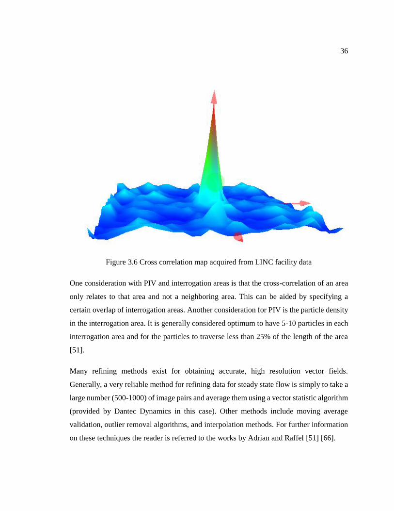
36

Figure 3.6 Cross correlation map acquired from LINC facility data

One consideration with PIV and interrogation areas is that the cross-correlation of an area

only relates to that area and not a neighboring area. This can be aided by specifying a

certain overlap of interrogation areas. Another consideration for PIV is the particle density

in the interrogation area. It is generally considered optimum to have 5-10 particles in each

interrogation area and for the particles to traverse less than 25% of the length of the area

[51].

Many refining methods exist for obtaining accurate, high resolution vector fields.

Generally, a very reliable method for refining data for steady state flow is simply to take a

large number (500-1000) of image pairs and average them using a vector statistic algorithm

(provided by Dantec Dynamics in this case). Other methods include moving average

validation, outlier removal algorithms, and interpolation methods. For further information

on these techniques the reader is referred to the works by Adrian and Raffel [51] [66].

37

Seeding fluid flow is a very important aspect of PIV technique. The seeds need to be similar

in density and momentum to the fluid so as to flow with it. The images taken and analyzed

in a PIV system are of these particles, and so in order to capture the fluid dynamics the

particles need to behave the same way. In addition to density matching, the particles need

to have enough surface area to reflect light to the camera. There is a fine balance for seed

particle choice for these reasons as characteristics that make ideal particles are sometimes

in opposition to each other. The seed particles used in the LINC facility are 10 μm

polystyrene microspheres. Polystyrene has a density of 1.05 g/cc, which is very similar to

that of water. There are many analyses on how to implement seeding particles to each

experimental application and fluid including accounting for characteristics such as settling

time and frequency response. Again, the reader is referred to Adrian’s book on the topic

for more information [51].

38

4 EXPERIMENTAL FACILITY

The LINC facility is a natural circulation facility with a fast response time and flexibility

for various experiments. Currently the facility accommodates two vertical heater rods

mounted through a top cooler plate. These rods heat water in the tank, which rises and

impinges upon the bottom surface of the cooling plate, cools, then drops to the bottom of

the tank only to be heated again. There is a laser mounted beneath the tank pointed upward

to create a plane of light between the heater rods. A high speed camera is mounted pointing

perpendicular to the rods and normal to the laser light plane to capture images of seed

particles illuminated by the laser. Figure 4.1 shows a labeled rendering of the LINC facility.

Figure 4.2 shows a closer view of the system and includes a rendering of the laser light

configuration.

39

Fig

ure

4.1

Ov

ervie

w o

f L

INC

fac

ilit

y

40

Figure 4.2 Rendering of LINC facility close up

4.1 Design Bases

4.1.1 Tank design

The design of the facility originated with the heater rod diameter, which was chosen to be

3.18 mm (3/8 in) diameter because this is a common size for fuel pins and also a common

size for cartridge heaters. From there, a suitable diameter for the tank was chosen based on

the number of rod diameters to ensure the effects of the wall on the flow would be

negligible. For this reason, a rectangular tank was designed with an inner diameter of 152

41

mm (6 in) on a side. The height of the tank was chosen to be 381 mm (15 in) inside from

the “floor” of the tank to the cooling plate surface. The pitch of the rods is adjustable, and

so the number of diameters between the heater rod and the wall in this design ranges from

6.5 to 1 in one direction and remains constant at 7.8 diameters in the other direction. A

sketch of the tank is shown in 1 Figure 4.3.

Figure 4.3 Tank sketch with dimensions

42

The tank was constructed of transparent acrylic which is 11.13 mm thick. This thickness

was chosen for strength and robustness and also for the convenience and benefit of having

the transparent tank bottom also be the mounting surface to a stand. This thickness allows

for the full weight of the water tank to rest on the oversized transparent bottom. This is

important because the laser is positioned underneath the tank pointing up to create a light

plane between the heater rods for the PIV system. Acrylic was chosen as the tank material

both for its strength and for its similar index of refraction to water.

4.1.2 Cooling Plate Design

The design of the cooling plate has accounted for more design time than any other

component of the LINC facility. It was desired to have the flexibility to be able to test

various rod pitches, but two issues complicated the design. The first was the desire to avoid

complex flow effects from a long channel in contact with the water and the second issue

was the cost with machining a custom cooling plate for every pitch desired. The design of

the cooling plate solves both of these issues by making the cooling plate in 2 pieces. The

top portion (side A) has all of the coolant channels, rod mount hardware, O-ring glands,

and tank mount holes while the bottom plate (side B) is simply a thin cap to contain the

coolant. A cross-section of the cooling plate assembly is shown in Figure 4.4 to clarify the

design of the plate. The portion of the bottom plate in contact with the water in the tank is

polished and flat all except for two holes for the heater rods which have a fit tolerance

small enough to be virtually flat across the entire plate. While the flat bottom plate only

has 2 holes in it, the top portion of the cooling plate has a channel cut into it in the center

with 8 mounting positions for each rod, in 6.35mm inch increments. This allows for fine

adjustment to various rod pitches, and just replacing the bottom plate for each pitch. In

order to ensure good conduction to and from the plate, it was made from Copper 110, which

is 99.9% pure. The technical drawings of the cooling plate are included in Appendix A (as

Figure 10.3, Figure 10.4, and Figure 10.5) and should be referred to for clarification of the

explanations herein. These drawings show the channel for the heater rods, the adjustment

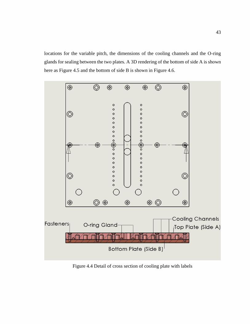
43

locations for the variable pitch, the dimensions of the cooling channels and the O-ring

glands for sealing between the two plates. A 3D rendering of the bottom of side A is shown

here as Figure 4.5 and the bottom of side B is shown in Figure 4.6.

Figure 4.4 Detail of cross section of cooling plate with labels

44

Figure 4.5 Rendering of side A of cooling plate

Figure 4.6 Rendering of side B of cooling plate

45

The top of side A has pipe threaded holes for fittings to be attached to the cooling water

lines from the chiller. As can be seen from Figure 4.5, the plate is split symmetrically along

the centerline of the rod channel. This means that there are two separate cooling channels

which are cooled symmetrically by splitting the flow from the chiller into 2 lines as shown

in Figure 4.7. Also shown in Figure 4.7 is how the colder (blue) lines start at the center and

the warmer water (red) leaves the plate toward the outside edge.

Figure 4.7 Cooling configuration of cooling plate

The cooler plate is attached to the acrylic tank using steel socket head cap screws which sit

flush with the top of the plate and screw into brass press-fit expansion inserts in the acrylic

tank. These brass inserts were pressed into holes drilled into the acrylic tank.

46

In between the cooling plate and the acrylic is a silicone foam gasket to seal the water in.

This silicone foam allows for all of the air in the tank to be eliminated so the water can

have total contact with the cooling plate. The two plates are attached together using small

screws which pass through side A and attach to threads cut into side B at several locations

(specified in Figure 10.5).

4.2 Experimental Equipment and Specifications

4.2.1 Heaters & Cooling

When choosing heater rods, preference was given to the diameter of fuel pin commonly

used in the nuclear industry (9.525 mm). It was desired to have rods long enough to be able

to analyze a long section of developed natural convective flow and so a heated length of

0.3048 m (12 in) was chosen. The heater rods used were manufactured by Bucan Electric

Heating Devices Inc. An example cross section of the heater rod is provided in Figure 4.8.

The diameter of the rods are 9.525 mm. They are 0.4064 m in total length with 0.3048m of

it uniformly heated, starting 6.35 mm (0.25 in) from the tip opposite the leads. A Type K

thermocouple was installed in the heater halfway along the heated region (0.15875 m from

the end opposite the leads) in the center of the Magnesium Oxide (MgO) core ceramic

(region 2 in Figure 4.8). The heater rod is sheathed in a thickness of 1 mm of INCOLOY-

800 (number 4 in Figure 4.8). The heater element is a spiral NiCr wire (number 1 in Figure

4.8) that is packed into the sheath approximately 0.13 mm from the wall (with MgO

between) (region 3 in Figure 4.8). The heater rods have an input voltage range of 0-100V

and an operational power range of 0-700W.

47

Figure 4.8 Cross section view of heater rod design. Image courtesy of Bucan

The power supplies used to power each rod are BK Precision® brand, model number

XLN10014. These have a voltage range of 0-100V and a current range of 0-14.4 A. They

have a readback accuracy of 0.05%+25mV which allows for accurate feedback of actual

power being used by the rods. These power supplies were chosen for their versatility and

precision. Also, since the power supplies monitor actual power usage there was no need to

acquire additional equipment to measure current and voltage. The power supplies are

programmable and can be controlled by a USB interface but for the purposes of the lab

they are manually adjusted using the built-in keypad and LCD.

The heater rods are held in place by custom clamps which are made from aluminum. These

clamps mount to the top of the cooler plate in any of several locations depending on the

desired pitch. Detailed information on the heater rod clamps can be found in Appendix A

in Figure 10.6 and Figure 10.7.

The chiller used is a Cornelius® brand, model number CH951A. It has a 1 horsepower

condensing unit, a reserve capacity of 18.9 gallons and an operating water temperature

range of 40-100°F. The secondary loop (cooling) flow rate is measured with an acrylic

rotameter with a steel float. The rotameter has a 25.4 cm viewing scale and a flow range of

0.76 - 8.33 L/min. The read-out precision of the rotameter is 0.038 L/min with an accuracy

of ±2.0%. With the system configuration in the LINC facility, the circulation rate in the

cooling water line is 3.03 L/min. This flow rate is largely governed by the pressure drop

across the cooling plate, tubing and fittings.

48

4.2.2 Instrumentation

In order to perform an energy balance on the facility, the temperature at various locations

were measured. These locations are as follows:

In the tank:

o One thermocouple mounted in the center of the tank at the height of the

center of the heated region of the rods.

o One thermocouple above and one below the center thermocouple at a

distance of 7.62 cm (3 in) from center.

In the cooling water line:

o One mounted into a “cross” fitting at both the inlet and outlet lines to the

cooling plate.

Temperature data was collected using a National Instruments™ CompactRIO model

number CRIO-9022 controller with a cRIO-9113 4-slot chassis. The chassis contains a 16-

channel thermocouple input module, model number NI 9213 which read in all

thermocouple data. The thermocouple data was processed and displayed using LabView.

A LabView program was written which collected temperature data from the 7

thermocouples (3 in the tank, 2 on secondary loop and 2 in heater rods), and created a

spreadsheet from the data, recording temperatures at a rate of 1 Hz. The spreadsheet

filename is automatically named based on the date and time of the experiment.

4.2.3 PIV System

The PIV system is a package from Dantec Dynamics which includes a laser, high speed

camera, timer box and DynamicStudio software. The laser is manufactured by RayPower,

model number 5000. The laser is Q-switched, has a wavelength of 532 nm and an output

power >5000mW. The laser has an entrance module, model number 9080X8941 which

creates the light sheet for illumination of the seed particles. The seed particles used are

49

Polysciences Polybead® Microspheres with a 10μm mean diameter with a coefficient of

variance of 10%.

4.3 Procedure and Set-up for Characterization Experiments

4.3.1 Thermal Equilibrium Analysis

A model was developed, using all of the information from section 3, to predict the

thermodynamic behavior of the LINC facility from startup to steady-state. This model was

written in Python [79]. The model first builds a library of material properties as functions

of temperature, length, or whatever is appropriate. This includes heat capacity, density,

viscosity and other properties, mostly of water. These functions are then used to create the

next level of functions which consist of things like the volumetric thermal expansion

coefficient and kinematic viscosity. The next level of functions uses the prior level to build

up to relevant parameters such as the Grashof number and Rayleigh number. Once the

hierarchy of functions is established, one can simply call a function like the Rayleigh

number and pass in a few parameters such as bulk fluid temperature, surface temperature

and characteristic length. This facilitates and simplifies the calculations for correlations

for the Nusselt number to find heat transfer coefficients and other important parameters for

characterizing the thermodynamic behavior of the system. The model numerically solves

for the surface temperature of the rods by first evaluating a range of possible temperatures

and finding the difference between the “left hand side”, hlhs, and the “right hand side”, hrhs,

at each temperature. In this case, the left hand side is shown in equation (4.1) and the right

hand side is shown in equation (4.2) which come from equations (3.40), (3.41), and (3.42).

ℎ𝑙ℎ𝑠 =

𝑞′′

𝑇𝑠 − 𝑇𝑏𝑢𝑙𝑘 (4.1)

50

ℎ𝑟ℎ𝑠 =

[ {0.825 +

0.387𝑅𝑎𝐿1

6⁄

[1 + (0.492 Pr)⁄9

16⁄]8

27⁄}

2

+ 0.97𝐿

𝐷] (𝑘

𝐿) (4.2)

The temperature range evaluated begins from the bulk temperature and proceeds in

increments of 1°C for 200 degrees. The model finds the minimum of the matrix of the

difference between hlhs and hrhs, then examines 4000 temperature increments in a range of

2 °C below to 2°C above the initial minimum temperature index. The minimum of this

matrix of the difference between hlhs and hrhs is then considered to be the surface

temperature for that time step. The surface temperature of the rod can be used to find the

Grashof and Rayleigh number at any point on the rod and indeed to analyze the profile of

Ra along the rod (see section 4.3.2 for further use and significance of this). In addition to

finding the surface temperature, the model uses equations (3.30), (3.36), and (3.38) to

calculate the heat removed by the plate. The model updates bulk water temperature and

coolant temperatures every time step based on the disparity between how much power the

rods are adding and the cooling plate is removing. Ultimately, equilibrium is reached by

the bulk fluid rising in temperature enough to increase the driving force to the cooling plate

such that Qin = Qout. The model proceeds until the difference between the heat removed by

the plate and the heat added by the heater rods is less than 0.001 W. The model records the

history of the system and returns a text file with the heater power, cooling plate removal

rate, bulk temperature and Gr and Ra at the top of the rod at each time step. In addition to

this data, the model records a profile of Gr and Ra as well as boundary layer thickness in

50 incremental locations along the heater rods.

For the thermal equilibrium analysis, the objective was to determine how well the model

created using the information from section 3 adequately represented reality. To begin, the

tank was left to equilibrate to room temperature by sitting for an adequate amount of time.

All bubbles were removed from the top of the tank by way of a needle inserted through the

gasket between the copper plate and the tank. This ensures uniform, symmetrical and

51

consistent heat transfer from the tank to the cooler plate. For the sake of this experiment,

the cooling plate was removed from the chiller loop while it cooled its reservoir. Once the

chiller reached its set-point, the cooler plate is added to the chiller coolant loop and started

at the same time the rods receive power. The power of the rods was recorded from the

power supplies, which was relatively constant over the experimental time. Another

parameter that was largely constant is the flow rate of water in the secondary loop from the

chiller. The flow rate of this loop is measured with a high-accuracy flow meter as described

in section 4.2.1. In order to find the heat removed by the coolant, the temperature of the

inlet and outlet coolant lines from the plate are measured in the center a “cross” fitting with

a probe-type thermocouple. Using the temperature difference and the water flow rate the

energy added to the coolant can be calculated and compared to the model results. The

temperature is also measured at the centerline of the heater rods and at 3 locations in the

tank specified earlier. All temperature measurements are recorded by LabView every

second and written to a data file. All of this information is then used to compare to the

thermodynamic model.

4.3.2 Boundary Layer Thickness Analysis

An important aspect of flow adjacent to surfaces is the boundary layer characteristics.

Knowledge about boundary layer properties can lend to predictions about diffusion, heat

transfer, turbulence and other defining characteristics of flow. The LINC facility has the

capability to study the boundary layer in a natural circulation environment in great detail.

One important property of the boundary layer is its physical thickness. This thickness will

increase as the Rayleigh number increases along a heated surface. Of particular interest is

when the boundary layer grows large enough that it is no longer isolated and begins to

interact with another surface or the boundary layer from another surface.

The model described in section 4.3.1 conveniently creates a function for Gr which can be

evaluated at any point x along the rod. This is used in Eckert’s equation (3.44) to determine

the boundary layer thickness at any point x along the rod. One of the driving design

52

characteristics of the LINC facility was the boundary layer thickness. It dictated the design

of the size of the tank, and consequently the cooling plate and the pitch adjustment positions

for the heater rod clamps. When designing the facility, it was desired that there be

flexibility in testing overlapping boundary layers between two heated rods, and so a good

design basis calculation was needed to estimate the thickness of said boundary layer.

In order to evaluate how accurately the LINC facility design matches the predictions using

Eckert’s equations for boundary layer thickness, a series of experiments were performed

to determine boundary layer thickness. The following is an outline of the procedure used

to collect data for the boundary layer analysis.

In the LINC facility, the polystyrene microspheres used to seed the flow have a density that

is slightly greater than that of water, so over a long period of settling such as overnight,

they may rest on the bottom of the tank. A custom stirring rod was designed from an

aluminum rod and some gasket material to stir and coax the seed particles into suspension.

The stirring rod fits through one of the heater rod holes so it is necessary to remove any

bubbles collected on the top plate as a result of the removal and re-insertion of the rod due

to displacement. Since this experiment relies on uniform cooling via direct contact with a

cooling plate mounted on top of the tank, all bubbles were removed prior to

experimentation. Sometimes when the tank water is cooling down, the water will naturally

contract and draw in air from the gap around the rods. This is easily remedied by staying

aware of cooling conditions and adding water as necessary. Once all seed particles were in

suspension and all air was evacuated from the top of the tank, the heaters and chiller were

turned on and the system was allowed to reach steady state. Generally, the system is

considered to be at steady state when the bulk fluid temperature does not change more than

1% in 10 minutes. The thermal equilibrium analysis presented here in section 5.1 details

how long it takes to get to steady state for several heater set points but generally equilibrium

was reached in about 2 hours of startup.

53

Once steady state conditions were established, the camera was positioned to focus on the

center plane between the two heater rods. This was accomplished by turning on the laser

and focusing the camera on the seed particles illuminated by the laser sheet between the

rods. The camera was calibrated using the known diameter of the heating rods so an image

was taken with room lights on and a scale factor was measured to translate pixels to

absolute distance. For the case of the LINC system, the flow rates are slow enough that the

camera shutter rates are more than adequate to get good image pairs for velocity

correlations. For this reason, for acquisition with the LINC system, the laser was simply

left on continuously while the camera collected images. If it is desired to capture periodic

behavior, a high frame collection rate can be used such as 100-500 Hz. For time-averaged

flow patterns, one can set the image pair collection rate to 1-20 Hz, which, when collecting

100-200 images at 1 Hz will give a representation of behavior over the course of several

minutes.

For the boundary layer characterization experiments, the camera was placed close enough

to the heater rods such that the frame of view encompassed approximately 40 mm from top

to bottom. 50 images were taken at the first location, where the bottom of the heater rods

were just barely touching the bottom of the view frame. Once the images were collected,

the camera was moved up using the camera mount system. The camera was moved the

same distance up as was visible in the scaled images collected at the first location in order

to attempt to construct a continuous vector field for the entire heated channel. Images were

collected at 7 vertical settings (marked to ensure repeatability) for each power setting. A

matrix of power settings was examined to start to characterize the system and see how

accurate the boundary layer predictions were. Table 4.1 shows the combinations of rod

powers chosen for the boundary layer analysis. The number in the test matrix refers to the

test case number used to identify it.

54

Table 4.1 Boundary Layer Experimental Test Matrix

Case # Right Heater

100W 200W 300W

Lef

t H

eate

r 100W 1 2 3

200W 4

300W 5

Once images are recorded they are transferred from the RAM buffer on the camera to

network storage system where they can be analyzed. The LINC facility uses equipment

and software from Dantec Dynamics. The Dantec software includes an auto-correlation

method which determines a vector for each interrogation area based on statistical

algorithms. For the experiments presented here, a 16x16 pixel interrogation area was used

because the camera was relatively close to the flow field, there were plenty of seed

particles, and a high resolution was desired to capture boundary layer information. Each

image pair is analyzed to get a vector field. In such vector fields there are inevitably

interrogation areas where there are invalid or substituted vectors where there was not

enough of a statistical confidence in the correlation. Much of this variability is eliminated

by using the software to average all of the vector fields to greatly increase the confidence

in the vector field values and eliminate random noise and variations.

4.3.3 Velocity Profile Analysis

Another important metric for analyzing flow patterns is the velocity profile. The model of

the system velocity profile near the heated rods consisted mostly of solutions to Eckert’s

equation (3.45). The velocity equation was evaluated at several locations along the heater

rod in order to gain an understanding of the velocity profile progression. The velocity

profile and the boundary layer are inherently linked since the boundary layer thickness (as

55

defined by Eckert and Jackson) is where the velocity profile drops to a threshold number.

Quantification of the velocity profile is achieved by calibrating a scale factor in an image

as explained earlier.

In order to compare the approximation by Eckert, measurements were taken at the same

conditions and locations along the rods as were used in the calculations. Since the shape of

the velocity profile was desired and not just the thickness of the boundary layer, 700 images

pairs were collected to obtain a cleaner vector field and only 2 sequential, 40mm view

fields were investigated for the case of each rod heated to 200W.

56

5 RESULTS AND DISCUSSION

5.1 Energy Balance Characterization

The energy balance was evaluated for 3 different symmetrical heat rates from the heater

rods: 200W, 300W and 400W (each rod). The principle metrics for comparing the energy

balance of the rod with the model were the bulk fluid temperature and the energy removed

by the plate. The model of the LINC system reached an asymptotic solution for the bulk

temperature and it was desired to know how well the behavior of the actual facility matched

the model. Figure 5.1 shows the bulk temperature equilibrium behavior for the system and

model for the rods at 200 watts each. Figure 5.2 shows the heat removed by the cooling

plate, as measured by the flow rate of the coolant and temperature change from inlet to

outlet of the plate. Figure 5.3 and Figure 5.4 show the equilibrium temperature and heat

transfer to the plate for a power of 300W to each rod while Figure 5.5 and Figure 5.6 show

the same for a power of 400W in each rod. A summary of the three energy balance cases

compared with the model are presented in Figure 5.7 and Figure 5.8. One interesting feature

of note in the 400W case, is the disturbances in the temperature and power. This was caused

by bubbles being released by the heater rods rising and collecting on the bottom of the

plate. When the bubbles were removed, the bulk tank temperature fell and the heat removed

by the plate shot up. The bubbles were removed three times in this experiment, with the

same result all three times.

57

Figure 5.1 Temperature equilibrium plot for 200W rod power

Figure 5.2 Power equilibrium plot for 200W rod power

58



59



60

Figure 5.7 Equilibrium temperature comparison summary

Figure 5.8 Equilibrium power comparison summary

61

As can be seen from the range of figures from Figure 5.1 through Figure 5.8 that the model

seems justified as a first approximation of the facility. It was noticed, however, that the

model is not capable of capturing some of the complex heat transfer mechanisms in the

actual facility. This makes sense for several reasons listed here:

1. The Nusselt number for the bottom of the cooling plate where it contacts the water

is based on the Rayleigh number of the plate only, which is 4 orders of magnitude

less than that of the Rayleigh number of the rod where it meets the plate. If the

Rayleigh number of the rod were used to find Nu of the plate (although this is

beyond the specified use case for the correlation), the model would over-predict the

cooling in the plate for most cases. This impingement effect is very apparent at

lower cooling rates, where the actual pool temperature is much lower than that

predicted by the model and in fact, lower than room temperature by as much as 7

°C. At the higher power of 400 W, the impingement seems a less dominant

phenomena than at lower powers, instead it seems the entire plate becomes more

significant to heat transfer with the larger temperature differential between the

cooling water and the bulk water temperature.

2. The cooling water enters the plate symmetrically on each side of the heater rod

channel, with the cold leg entering the center region of the plate and the hot leg

leaving at the outer edge of the plate. This means that the buoyant plume mentioned

in (1) impinges on the coldest portion of the cooling plate, maximizing the cooling

effect of the phenomena.

3. The model makes no effort to account for cooling by natural convection on the

outside of the tank due to conduction through the acrylic. There are also minor

losses such as conduction up through the heater rod into the rod clamps, water

evaporating from the cooling plate on top, or conduction from the tank to the frame

that are not accounted for by the model. For the case of heat loss from the acrylic

62

tank to the air, this effect is expected to contribute more significantly to the disparity

of the experimental data to the model at higher powers and tank temperatures, and

indeed this is the case where one can see in Figure 5.6 the power drawn out by the

cooling plate is less than that provided by the heater rods. It makes sense that even

though the tank is being heated at lower power levels, the equilibrium temperature

is barely above room temperature and so little to no driving force exists to drive

heat transfer to the room. As the power level increases, the equilibrium tank

temperature also increases and the temperature differential between the bulk fluid

and the room becomes noticeable.

5.2 Boundary Layer Characterization

The boundary layer analysis was perhaps the most subjective and qualitative of the analyses

performed in this study. The boundary layer can be defined as the distance from the surface

at which the velocity is a certain fraction of the bulk fluid. Eckert proposes that the

boundary layer edge was located where V=0.99Vbulk, but in a channel it is not as clear how

the bulk fluid velocity can be defined. Different methods were employed to attempt to

develop a consistent and definite method of determining the boundary layer thickness. One

difficulty of the determination is the need to distort the image to be able to analyze it. Figure

5.9 shows a full length surface plot of V in the channel between the heated rods at a power

setting of 200W with an aspect ratio that is to scale. The color coding is proportional to V

where blue in this case is low to zero velocity and red represents higher velocities. This

aspect ratio is unwieldy and yields little data so further images will be shown with a more

appropriate scaling to best view results. Figure 5.10 shows a different aspect ratio, where

the velocity behavior is more apparent.

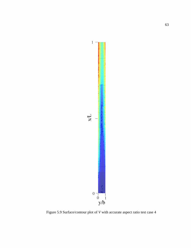
63

Figure 5.9 Surface/contour plot of V with accurate aspect ratio test case 4

64

Figure 5.10 Surface/contour plot of V for full profile test case 4

In Figure 5.10, one can see slight discontinuities where vector fields were stitched together

but the full profile is remarkably continuous for being taken in seven segments over the

course of about 2 hours. The discontinuities are likely the result of slight camera

misalignment during adjustment. The channel between rods being 9.42 mm wide, a

difference of even 1 mm in adjustment laterally can alter the alignment by more than 10%.

In order to compare to Eckert, a consistent method of analysis was developed wherein the

vector field was evaluated logically using a computer. The velocity in the center of the

entrance region was averaged across a 4X3 grid of vectors and each vector in the map was

divided by that average entrance velocity. If the value exceeded 50, then a 1 was assigned

to the cell, with a 0 being assigned should the value be less than 50. This meant that the

65

edge of the boundary layer was found when 0.02V=Ventrance. This logic was applied to all

five rod power combination test cases. This threshold method, plotted against the boundary

layer thickness predicted by Eckert is shown for all test cases in Figure 5.11 through Figure

5.15. Figure 5.16 is shown alongside the threshold method to show what a 2D

representation of the velocity map looked like.

For all cases, the experimental boundary layers are similar to what Eckert and Jackson

predicted in 1950. Case 5 is almost exact in its agreement with Eckert until there is a

discontinuity from one camera location to the next.

66

Figure 5.11 Boundary layer comparison

Case 1


Case 2

67


Case 3


Case 4

68


Case 5

Figure 5.16 Colorized surface plot of V

for test case 5

69

Overall, the design basis calculations for the LINC facility with regards to the boundary

layer thickness seem to be justified and have provided a reasonable estimate of the

boundary layer thickness in the facility. The data seems somewhat rough on some plots,

and there seemed to be some asymmetrical heating effects, but overall the facility design

appears to be right in line with the behavior it was predicted to have in the boundary layer.

There are several possible reasons why the measured boundary layer thickness deviated

from the predicted results. The foremost of these is the applicability of Eckert and

Jackson’s expression to water and a cylinder. The expression is most relevant for fluids

with a Prandtl number of 1, and it was a stretch to apply it to water (Pr of about 7). In

addition, there is something called the transverse curvature effect that causes flow adjacent

to a cylinder to differ from that adjacent to a flat plate. The effect becomes more

pronounced as the ratio of δ/D nears unity or greater and is exacerbated further at large x/D

where the boundary layer is fully developed. Sparrow and Gregg suggest that the

correlations for a flat plate can be used on a vertical cylinder if the condition in equation

(5.1) holds.

𝐷

𝐿≥

35

𝐺𝑟𝐿1 4⁄

(5.1)

For the case of the LINC facility heater rods, this condition is not met and so the transverse

curvature has an appreciable effect on boundary layer thickness and increase in heat

transfer. For these reasons, it is actually somewhat surprising that the results align as well

as they do. For an investigation of the transverse curvature effect on the boundary layer

thickness one would likely need to either increase the pitch or examine the outside of one

of the rods (as opposed to inside the channel) to examine a full length profile without

overlap from the other heater rod boundary layer.

As mentioned above, the boundary layer thickness data gathered in this study is fairly

coarse and the convention used to determine the boundary layer edge (0.02V=Ventrance) is

somewhat arbitrary. If, for example, the definition of 0.01V=Ventrance were chosen to

70

indicate the boundary layer edge, the boundary layer profiles would shift slightly up in the

channel but still exhibit the same basic shape. For this reason, a different method of

determining boundary layer thickness should be investigated. Due to the more complex

nature of the channel between two rods, the new method should be more sophisticated than

simply a threshold of velocities. The new method could consist of a multiple of the distance

between the velocity maximum and the inflection point of the velocity curve (see the next

section for such a curve example) taking the form of equation (5.2) where C would be a

constant in the range of 2.

𝛿 = 𝐶(𝑦𝑖𝑛𝑓 − 𝑦𝑚𝑎𝑥) + 𝑦𝑚𝑎𝑥 (5.2)

Investigating the validity of this new definition of the boundary layer thickness is beyond

the scope of this work but it is of interest to the author and of value to include in future

work.

5.3 Velocity Profile Characterization

The velocity profile was measured in detail for one heating case of 200W to each rod. The

surface temperature associated with this power level at equilibrium was 58°C, however

some asymmetry was noticed in the rod temperatures which had actual surface

temperatures of 57.6°C and 58.6°C. A surface plot of the velocity V is shown Figure 5.17.

The plot shows some asymmetry in the velocity maximum which is likely related to the

temperature asymmetry, though overall the data is very clean and smooth, showing the

formation of the boundary layer in the first 100 mm of channel between the heater rods. If

one examines the center “valley” region of the surface plot, a nascent channel bulk velocity

can be seen, which is real and quantifiable but clearly outside of the boundary layer. This

is partly what introduces difficulty in defining a boundary layer thickness in terms of bulk

velocity because further along the rod that center region will be indistinguishable from the

boundary layer edge.

71

Figure 5.17 Surface plot of velocity profile for 200W power

In order to compare to the design calculations using Eckert’s equations, the velocity map

shown in Figure 5.17 was sampled at 10 locations from the leading edge of the heater rod:

3.05 mm, 13.22 mm, 23.07 mm, 32.93 mm, 43.08 mm, 53.12 mm, 63.04 mm, 73.20 mm,

83.05 mm, and 90.75 mm. These values were inserted into equation (3.45) along with the

surface temperature of the rod and the bulk temperature of the tank to directly compare the

same locations and conditions in the model and experiment. Figure 5.18 shows the velocity

profile progression for one side of the channel at each of the ten x coordinates.

72

Figure 5.18 Velocity profile development in absolute units a 200W

As can be seen in Figure 5.18, the velocity profile develops through a consistent

progression from the entrance region into the full-bodied velocity profile shape shown at

90.75mm. Each profile drops asymptotically to a velocity which can be thought of as the

channel bulk velocity. Figure 5.19 shows the same information as Figure 5.18, except it

has been normalized by dividing each velocity by the maximum velocity value in the array

(found in the profile of the 90.75 mm position). The x axis was normalized by the boundary

layer. For the velocity cases, it was assumed that the boundary layer edge was at the center

of the channel due to the subjective nature of the actual boundary (see the preceding section

for this discussion). The same profiles as predicted by the model are shown in Figure 5.20.

These are normalized by the actual boundary layer thickness predicted by equation (3.44)

by necessity since the nature of the velocity equation makes it only valid in the range 0 ≤

y ≤ δ.

73

Figure 5.19 Normalized velocity profile development at 200W

Figure 5.20 Velocity profile from Eckert

74

Comparing Figure 5.20 with Figure 5.19, it is observed that the two profile progressions

share similarities in shape but also exhibit some important differences. One difference

between the two is the lack of any channel bulk velocity from the model results. This is

expected as the profile by Eckert was evaluated only from 0 to δ, and Eckert designed his

model with the assumption that the boundary layer edge occurred when V=0.99Vbulk, and

Vbulk was assumd to be 0 in the model. In addition to the boundary layer edge behavior,

there are differences between the model and experimental results with regard to maximum

velocity progression. There seems to be an asymptotic value for the boundary layer

maximum velocity, whereas the maximum velocity in the experimental results appears to

be simply proportional to the distance from the leading edge. This difference can possibly

be attributed to the method in which Eckert’s equation was evaluated, which was by

assuming the surface temperature of the rod was uniform. In the experimental facility, even

though the heater rods have uniform heat flux in isothermal conditions (such as right at

startup), this will likely change as a boundary layer develops and flow begins. This is

because as the water is heated, and begins to rise, it continues to gain energy from the rod

and heat further. The heat transfer from the rod to the water is driven by a temperature

differential between the bulk fluid and the rod temperature. So, one would expect the heat

flux to shift slightly downward toward the colder water entering the channel and boundary

layer, and the temperature of the rod to shift up slightly at higher locations along the

channel proportional to the driving force provided by warmer water temperatures in the

boundary layer. For these reasons, it is in fact reassuring to see this difference between the

results from the model and those of the experimental facility. It should be noted that the

heat flux may actually shift up due to increased Ra and higher Nu at locations further along

the rod.

Another apparent difference between the model and experimental results is the relative

width of the velocity profile. The model profile is noticeably narrower than the

experimental one. This is investigated further in Figure 5.21, Figure 5.22, and Figure 5.23

where the normalized velocity profile of the model and experimental values are plotted

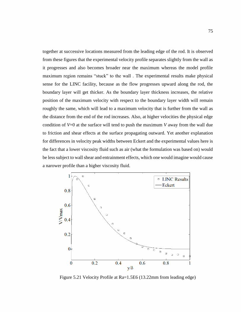
75

together at successive locations measured from the leading edge of the rod. It is observed

from these figures that the experimental velocity profile separates slightly from the wall as

it progresses and also becomes broader near the maximum whereas the model profile

maximum region remains “stuck” to the wall . The experimental results make physical

sense for the LINC facility, because as the flow progresses upward along the rod, the

boundary layer will get thicker. As the boundary layer thickness increases, the relative

position of the maximum velocity with respect to the boundary layer width will remain

roughly the same, which will lead to a maximum velocity that is further from the wall as

the distance from the end of the rod increases. Also, at higher velocities the physical edge

condition of V=0 at the surface will tend to push the maximum V away from the wall due

to friction and shear effects at the surface propagating outward. Yet another explanation

for differences in velocity peak widths between Eckert and the experimental values here is

the fact that a lower viscosity fluid such as air (what the formulation was based on) would

be less subject to wall shear and entrainment effects, which one would imagine would cause

a narower profile than a higher viscosity fluid.

Figure 5.21 Velocity Profile at Ra=1.5E6 (13.22mm from leading edge)

76

Figure 5.22 Velocity Profile at Ra=5.4E7 (43.1mm from leading edge)

Figure 5.23 Velocity Profile at Ra=5E8 (90.75mm from leading edge)

77

The absolute magnitude of the velocity profiles were different than those predicted by

Eckert by roughly a factor of 7 (Eckert predicting the higher values), though this is

understandable for a few reasons. The equations developed by Eckert were intended for

use on a flat plate. In addition, the formulas presented by Eckert were assumed to be valid

for Gr > 1010 and Pr close to unity. Both of these conditions place the work done here

technically out of the bounds of the formulation as water has a Prandtl number of roughly

7 and the velocity profiles measured here had a range of Ra from 107 to 109. Finally, the

geometry of the LINC facility is fundamentally different from the general geometry

configuration used to derive the velocity profile approximation in that it is not open at the

top of the free convection region but rather it impinges on a cold surface, the facility uses

2 adjacent heater rods between which the velocity was measured, and again, the heated

surface is a cylinder rather than a plate. There is a fundamental difference in the fluids used

in many experiments in natural convection such as air and water. For a gas like air, the

viscosity increases as temperature increases, but with water, the opposite is true. This could

also explain the difference between the velocity profile magnitude given by Eckert and the

experimental value since the evaluation by Eckert was carried out for a fluid with Pr close

unity.

5.4 The Nusselt Number and the Transverse Curvature Effect

A preliminary assessment of the Nusselt number vs. Rayleigh number was also performed

using the experimental results from the thermal equilibrium cases. The temperature of the

surface was calculated using the measured centerline temperature and the equations from

section 0and the Nusselt number was found using the rod power and the definition of the

convective heat transfer coefficient. The results were plotted against the Rayleigh number

at the same location along the rod and compared against previous work. This plot and

comparison is shown in Figure 5.24 where the results from Fujii [25] were experimental,

the results labeled Eckert is from the correlation developed by him and Jackson in 1950 [9]

and data labeled Churchill was calculated from the Nusselt correlation used in the

78

thermodynamic model of the LINC system presented in equation (3.40). Both correlations

used the actual experimental temperatures of the bulk fluid and rod surface. The red

markers are the Nusselt numbers measured at each heating case, with error bars.

Figure 5.24 Nu vs. Ra for current work compared with prior work

The results presented in Figure 5.24 are interesting for several reasons. First is that the

experimental results for Nu are higher than the results obtained by Fujii and those predicted

by Eckert. This can likely be explained by differences in geometry used. Eckert and

Jackson developed their correlation for a flat plate geometry. While Fujii’s experiments

were performed on a vertical cylinder in water, the radio of L/D for his system was

approximately 12.2 whereas the same ratio for the heater rods in the LINC facility is

approximately 31.8. There is a transverse curvature effect on the heat transfer from a

cylinder wherein the heat transfer is amplified with larger L/D. For this reason Fujii and

79

Uehara provided an upward correction for the Nusselt number for a plate when applied to

a cylinder (presented as equation (3.41)). Given this, the higher Nusselt number of the

LINC facility seems justified compared with prior data and the use of Churchill’s flat plate

correlation with the correction factor seems to approximate the facility well enough.

Another interesting point on the graph is the jump in the trend from the 300W to 400W

cases. It would appear that the large transverse curvature effect also contributed to an

earlier than expected transition to the turbulent regime. Fujii’s results indicated this

transition as being in the range of Ra near 1010.2 and here it appears to have occurred closer

to Ra = 109.4. Again, this is likely the result of the transverse curvature effect and should

be investigated further in future work.

5.5 Temperature Profiles

While the system was at steady state for the thermal equilibrium characterization, a

temperature profile was measured for each case from the surface to the wall. These profiles

are presented here in Figure 5.25, Figure 5.26, and Figure 5.27 where the surface

temperature was added based on a calculation from the centerline thermocouple due to the

sheathed nature of the tank thermocouples.

80

Figure 5.25 Temperature profile for 200W symmetrical heating case

Figure 5.26 Temperature Profile for 300W symmetrical heating case

81

Figure 5.27 Temperature profile for 400W symmetrical heating case

While the spatial resolution of the thermocouple measurements is low, there is still valuable

information that can be obtained from these temperature profile plots. First, it is interesting

to see just how uniform the temperature in the tank is outside of the boundary layer. For

all three heating cases, the temperatures of the thermocouples outside of the boundary layer

are within 1°C of each other. This indicates excellent mixing conditions in the bulk fluid

and the absence of any wall effects on the boundary layer. As a comparison, when the

heater rods and cooling plate are turned off, the water tends to stratify based on

temperature, leading to a temperature difference of up to 10°C in the 150 mm between the

top and bottom thermocouples. Another feature one might notice on these temperature

profile plots is the thermal boundary layer thickness and how much it varies between cases.

While it is certainly expected to have a thicker thermal boundary at higher heat rates from

the rods, the differences in these plots are primarily from the inability to obtain precise

measurements by pushing the thermocouples in by hand. This was mostly due to the fact

that neither the thermocouples nor the fitting they are mounted into were perfectly square

82

with the tank, so over a distance of 6 cm, sometimes the thermocouple tip was somewhat

tangential to the heater rod as opposed to normal to the surface. Due to the limitations on

acquiring an accurate temperature profile, Figure 5.25, Figure 5.26, and Figure 5.27 should

be considered mostly qualitatively for the shape of the curve and how uniform the bulk

fluid temperature is. The qualitative shape is in agreement with previous temperature

profile measurements [25]. It will be a consideration for the future to implement a more

precise temperature profile measurement system.

83

6 CONCLUSION

6.1 Observations

The LINC facility has been observed to perform as it was designed to do. The natural

circulation loop starts up and reaches steady state quickly, reliably and consistently. The

cooling plate design allows for varying of the rod pitch for the minor cost of a flat new

bottom plate.

The system behavior compares fairly well with the model developed to describe the

thermodynamics of the system. The cooling plate effectiveness was not captured by the

model for several reasons, the most significant of which is the inability of the model to

capture the cooling effect of the buoyant plume impinging on the center of the cooling

plate. This caused the predicted steady state bulk temperature to be higher than the actual

value measured experimentally. The case where both rods were powered at 400W, the

temperature of the model and experimental results were nearly identical, but looking at the

power removed by the plate, this appears to be largely from heat losses to the environment.

The expression provided by Eckert and Jackson for the boundary layer thickness was

compared with measured values from the facility. The boundary layer thickness tends to

be qualitative in nature unless it is defined in terms of bulk fluid velocity. In this work, the

boundary layer thickness was defined as the distance from the surface where 0.02V=Ventrance

where Ventrance was defined as the average velocity in a region at the center of the entrance

region of the channel formed by the heater rods. Using this definition, the boundary layer

thickness for series of five heating rates was evaluated and compared to the values

predicted by Eckert. The boundary layer thickness in the LINC system was found to be in

agreement with the predicted thickness, thus validating the design basis calculations and

confirming the usefulness of the LINC facility for collecting important thermal hydraulic

data with regard to boundary layer thickness.

84

The shape of the velocity profile created by the heater rods in the LINC system was found

to be in general agreement with the predictions by Eckert with a few exceptions of profile

progression behavior and peak width which have been determined to be mostly from over-

simplified assumptions used to calculate the predicted velocity profile and the fact that the

equations by Eckert were intended to be used for a fluid near Pr = 1.

The approximation of the Nusselt number by Churchill and Chu used in the model appears

to be justified, and the Nusselt number seems to be augmented due to the transverse

curvature effect of these rods.

6.2 Relevance of Work

The results of this paper confirm the value of the LINC facility for characterizing natural

circulation flow. The behavior of the system is in general agreement with the design basis

calculations used to design it. The flexibility and uniqueness of the system will allow for

the contribution of much needed experimental data in the field of natural circulation

adjacent to heated vertical cylinders and in channels between such cylinders. Of particular

value is the application of experimental data from this facility to natural convection

analysis and design for the nuclear industry. As mentioned in the introduction, natural

convection is a phenomena of great interest for passively safe system design. A deeper

understanding of natural convection phenomena, specifically that adjacent tonlong, heated

cylinders in water is clearly of great value.

While many similarity analyses and numerical calculations have been carried out over the

years on the subject of natural convection along vertical, heated plates and cylinders in

open flow and channel flow, there is a disproportionately smaller amount of experimental

data for the same subject. The LINC facility will be used to provide much-needed data to

the body of science for further refinement of the understanding of natural convection in

these configurations.

85

6.3 Experimental Limitations

There are clear limits on the applicability of the model used to design the system. The heat

transfer portion of model does not account for heat exchange with the environment, it does

not account for the oscillatory nature of the chiller, nor does it find the temperature profile

of the heater rods. In addition, the models used by Eckert and Jackson to determine the

boundary layer thickness and velocity profiles was not intended for use in such a

configuration, specifically with regards to Pr of the fluid and geometry of the system. As

the heat balance model and equations by Eckert and Jackson were used as a tool to design

and size the LINC facility, they were not meant to be comprehensive and exact.

As far as physical limitations of the LINC facility, there are a few that limit experimental

results. The first is the inability to obtain a full-length, continuous vector field of the

channel between the heater rods. This is mostly due to the small seed particles reflecting

such a small amount of light that by the time the camera is moved far enough away for a

full-field view, the light has attenuated enough to diminish detail in particle images. There

is also a resolution consideration for the camera where it wouldn’t be able to obtain

meaningful data for interrogation areas less than 1 mm if it were at such a wide field of

view. Considering that the channel is only 9.43 mm wide, this would make the vector

profile resolution very poor. For comparison, the results in section 5.3 have approximately

42 interrogation areas in the y direction between the heater rods because the camera was

placed close enough to capture only 40 mm of the channel in the x direction. While a

camera with a higher resolution would help in this regard, the previous issue of light

attenuation would limit the benefit derived from a higher resolution camera.

Another limitation of the LINC facility in its current state is the tendency of the laser sheet

between the rods to converge higher up the rod channel, leaving shadows near the rod

surface. This results in a lack of data in the shadow region as no particles are being

illuminated to correlate. The shadowed region can be as large as 2 mm at the top of the

heated region. The issue is being investigated to determine the cause and a solution.

86

As mentioned in section 5.5, the temperature profiles obtained, while valuable, were still

crude. The temperature profile was obtained by inserting a thermocouple into the tank

through a fitting. The thermocouple probes have such a small diameter (1.58 mm) that they

inevitably get bent, and the fitting that the thermocouple is mounted to is not perfectly

normal to the tank wall. This configuration led to large enough margins of error in the

temperature profile measurement to be unusable for boundary layer thickness analysis.

6.4 Future Work

There is much work to be done with the new natural convection facility that has been

constructed. To begin, a study can be done to examine more closely the difference between

the model of the cooling plate and the actual performance. The model was constructed

using correlations that have been used for decades for natural circulation flow on the

underside of a flat plate, though no mention could be found concerning adapting said

correlation in the presence of buoyant plume impingement. The LINC facility could be

used to see if, indeed this plume is having the enhanced cooling effect, as the author

suspects.

Further comparisons for velocity profiles are important for characterizing the unique flow

properties of the system. Vliet and Liu [80] have presented some data for water adjacent to

a vertical plate that seems to be one of the few data sets available for water adjacent to a

natural circulation surface, though the data they present is from a range of Ra beyond that

of the normal operating conditions of the LINC facility. Since experimental data about the

velocity profile in natural circulation conditions with water is clearly scarce, future work

with the LINC facility will surely include publication of velocity profile and flow

development behavior for a variety of conditions.

In addition to examining cooling plate behavior and velocity profiles, the LINC facility

should be used in the future to examine how vertical, heated cylinders interact in natural

convection conditions. Specifically, it would be of great value to determine the effect that

87

a power offset between the heater cylinders would have on boundary layers, Nusselt

number, and flow velocity patterns normal to the cylinder. This is of special interest in the

nuclear industry as nuclear fuel rods are cooled via natural convection in spent fuel pools

and some reactor designs have incorporated natural convection as the primary coolant

driving force. To be able to accurately model behavior in channels where a power offset is

present would be of great value to the nuclear industry.

While the values of Nu vs. Ra for the LINC facility were compared to previous work, only

4 experimental data points were obtained, and in order to test the hypothesis of augmented

Nu and shortened laminar region due to the transverse curvature effect, more experiments

over a wider range of conditions should be performed.

While the subject of velocity profiles and boundary layer profiles were examined in this

study, a detailed treatment of temperature profiles in the boundary layer was largely

unaddressed. This was primarily due to the lack of a current experimental setup for

acquiring such data. A better understanding of temperature profiles in a configuration such

as exists in the LINC facility would be of great value to the community and would be an

appropriate extension of velocity profile data acquired as well. In order to obtain high

resolution temperature gradients near the rods perhaps a Laser-Induced Fluorescence (LIF)

system can be implemented in the future for the temperature profile study.

Finally, this study has discussed the difficulty and seemingly arbitrary nature of the

boundary layer thickness adjacent to a heated vertical surface under natural circulation

conditions. It is of interest to pursue a more refined definition of the boundary layer

thickness than simply the location where the velocity is a fraction of the bulk velocity. As

mentioned before, a new method, perhaps using the maximum velocity location and the

inflection point in the velocity profile can be used to define the boundary layer edge. This

evolved definition of the boundary layer can be used to develop a new correlation to predict

boundary layer thickness based on Ra and curvature.

88

7 WORKS CITED

[1] I. William D. Magwood, "Report to Congress on Small Modular Nuclear

Reactors," U.S. Department of Energy, Washington, DC, 2001.

[2] IAEA, "Status of Small Reactor Designs Without On-Site Refuelling,"

International Atomic Energy Agency, Vienna, 2007.

[3] U.S. Department of Energy Office of Nuclear Energy, "SMR Factsheet," February

2010. [Online]. Available:

http://nuclear.energy.gov/pdfFiles/factSheets/2011_SMR_Factsheet.pdf.

[Accessed 21 March 2012].

[4] C. W. Forsberg, "Worldwide Advanced Nuclear Power Reactors with Passive and

Inherent Safety: What, Why, How and Who," Oak Ridge National Laboratory,

Oak Ridge, 1991.

[5] L. Lorenz, "Ueber das Leitungsvermögen der Metalle für Wärme und

Electricität," Annalen der Physik , vol. 249, no. 8, pp. 582-606, 1881.

[6] V. H. H. Lorenz, "Die Wärmeübertragung voneiner ebene, senkrechten Platte an

Öl bei natürlicher Konvektion," Zeitchr. f. techn. Physik, vol. 15, pp. 362-366,

1934.

[7] A. P. Colburn and O. A. Hougen, "Studies in Heat Transmission," Journal of

Industrial and Engineering Chemistry, vol. 22, p. 522, 1930.

[8] W. Elenbaas, "Heat Dissipation of Parallel Plates by Free Convection," Physica ,

vol. 9, no. 1, pp. 1-28, 1942.

[9] E. R. G. Eckert and T. W. Jackson, "Analysis of Turbulent Free-Convection

Boundary Layer on Flat Plate," NACA, Cleveland, 1950.

[10] T. v. Kármán, "On Laminar and Turbulent Friction," NACA, Washington, 1946.

89

[11] S. Ostrach, "Laminar Natural-Convection Flow and Heat Transfer of Fluids

Without Heat Sources in Channels with Constant Wall Temperatures," NACA,

Washington, 1952.

[12] S. Ostrach, " An analysis of laminar free-convection flow and heat transfer about

a flat plate parallel to the direction of the generating body force," National

Advisory Committee for Aeronautics, Cranfield, 1952.

[13] E. M. Sparrow and J. L. Gregg, "Laminar-Free-Convection Heat Transfer from

the Outer Surface of a Vertical Circular Cylinder," Transactions of the American

Society of Mechanical Engineers, vol. 78, pp. 1823-1829, 1956.

[14] E. M. Sparrow and J. L. Gregg, "Laminar Free Convection From a Vertical Plate

with Uniform Surface Heat Flux," Transactions of the American Society of

Mechanical Engineers, vol. 78, pp. 435-440, 1956.

[15] K. Millsaps and K. Pollhausen, "The Laminar Free-Convective Heat Transfer

From the Outer Surface of a vertical Circular Cylinder," Journal of Aeronautical

Sciences, vol. 25, pp. 357-360, 1958.

[16] J. R. Bodoia and J. F. Osterle, "The Developmet of Free Convection Between

Heater Vertical Plates," Journal of Heat Transfer, vol. 84, no. 1, pp. 40-44, 1962.

[17] H. R. Nagendra, M. A. Tirunaryanan and A. Ramachan, "Laminar Free

Convection from Vertical Cylinders with Uniform Heat Flux," Journal of Heat

Transfer, vol. 92, no. 1, pp. 191-195, 1970.

[18] T. Fujii and H. Uehara, "Laminar Natural-Convective Heat Transfer from the

Outer Surface of a Vertical Cylinder," International Journal of Heat and Mass

Transfer, vol. 13, pp. 607-615, 1970.

[19] W. Aung, L. Fletcher and V. Sernas, "Developing Laminar Free Convection

Between Vertical Flat Plates with Asymmetric Heating," International Journal of

Heat and Mass Transfer, vol. 15, no. 11, pp. 2293-2308, 1972.

90

[20] T. Cebeci, "Laminar-Free-Convective-Heat Transfer from the Outer Surface of a

Vertical Slender Circular Cylinder," Heat Transfer: Proceedings of Fifth

International Conference, vol. 3, pp. 15-19, 1974.

[21] J. P. Narain, "Free and Forced Convective Heat Trasnfer from Slender Cylinders,"

Letters in Heat and Mass Transfer, vol. 3, pp. 21-30, 1976.

[22] H. R. Nagendra, M. A. Tirunarayanan and A. Ramachandran, "Free convection

heat transfer from vertical cylinders and wires," Chemical Engineering Science,

vol. 24, pp. 1491-1495, 1969.

[23] R. Cheesewright, "Turbulent Natural Convection from a Vertical Plane Surface,"

Journal of Heat Transfer, vol. 90, no. 1, pp. 1-8, 1968.

[24] Kato, "On the Turbulent Heat Transfer by Free Convection from a Vertical Plate,"

International Journal of Heat and Mass Transfer, vol. 11, pp. 1117-1125, 1968.

[25] T. Fujii, M. Takeuchi, K. Suzaki and H. Uehara, "Experiments on Natural-

Convection Heat Transfer From the Outer Surface of a Vertical Cylinder to

Liquids," International Journal of Heat and Mass Transfer, vol. 13, pp. 753-787,

1970.

[26] W. J. Minkowycz and E. M. Sparrow, "Local Nonsimilar Solutions for Natural

Convection on a Vertical Cylinder," Journal of Heat Transfer, vol. 96, no. 2, pp.

178-183, 1974.

[27] H. B. Mason and R. A. Seban, "Numerical Prediction for Turbulent Free

Convection from Vertical Surfaces," International Journal of Heat and Mass


[28] S. W. Churchill, "Correlating equations for laminar and turbulent free convection

from a horizontal cylinder," International Journal of Heat and Mass Transfer, pp.

1049-1053, 1975.

91

[29] R. Cheesewright and K. S. Doan, "Space-Time Correlation Measurements in a

Turbulent Natural Convection Boundary Layer," International Journal of Heat

and Mass Transfer, vol. 21, pp. 911-921, 1978.

[30] W. K. George Jr. and S. P. Capp, "A Theory for Natural Convection Turbulent

Boudnary Layers Next to Heated Vertical Surfaces," International Journal of


[31] E. Griffiths and A. H. Davis, "The Transmission of Heat by Radiation and

Convection, D.S.I.R. Special Report 9," British Food Investigation Board,

London, 1922.

[32] S. V. Ptankar and D. B. Spalding, Heat and Mass Transfer in Boundary Layers,

2nd Ed., London: Intertext Books, 1970.

[33] T. S. Chen and C. F. Yuh, "Natural Convection Along a Vertical Cylinder,"

International Journal of Heat and Mass Transfer, vol. 23, no. 4, pp. 451-461,

1980.

[34] W. M. To and J. A. C. Humphrey, "Numerical simulation of buoyant, turbulent

flow - 1. Free convection along a heated, vertical, flat plate," International

Journal of Heat and Mass Transfer, vol. 29, no. 4, pp. 573-592, 1986.

[35] K. Velusamy and V. K. Garg, "Transient natural convection over a heat

generating vertical cylinder," International Journal of Heat and Mass Transfer,

vol. 35, no. 5, pp. 1293-1306, 1992.

[36] M. R. Gavara, P. Dutta and K. N. Seetharamu, "Mixed convection adjacent to

non-isothermal vertical surfaces," International Journal of Heat and Mass

Transfer, vol. 55, no. 17-18, pp. 4580-4587, 2012.

[37] P. Ganesan and H. P. Rani, "Transient natural convection along vertical cylinder

wth Heat and Mass transfer," Heat and Mass Transfer, vol. 33, pp. 449-455, 1998.

92

[38] T. Yilmaz and S. M. Fraser, "Turbulent natural convection in a vertical parallel-

plate channel with asymmetric heating," International Journal of Heat and Mass

Transfer, vol. 50, pp. 2612-2623, 2007.

[39] T. Tsuji and Y. Nagano, "Velocity and Temperature Measurements in a Natural

Convection Boundary Layer Along a Vertical Flat Plate," Experimental Thermal

and Fluid Science, vol. 2, pp. 208-215, 1989.

[40] J. H. Merkin, "Natural-convection boundary-layer flow on a vertical surface with

Newtonian heating," International Journal of Heat and Fluid Flow, vol. 15, no. 5,

pp. 392-398, 1994.

[41] M. Z. Abedin, T. Tsuji and J. Lee, "Turbulence characteristics and vortical

structures in combined-convection boundary layers along a heated vertical flat

plate," International Journal of Heat and Mass Transfer, vol. 55, pp. 3995-4002,

2012.

[42] S. C. Saha, R. J. Brown and Y. T. Gu, "Prandtl number scaling of the unsteady

natural convection boundary layer adjacent to a vertical flat plate for Pr >1 subject

to ramp suface heat flux," International Journal of Heat and Mass Transfer, vol.

55, no. 23-24, pp. 7046-7055, 2012.

[43] M. Miyamoto, Y. Katoh, J. Kurima and H. Sasaki, "Turbulent Free Convection

Heat Transfer from Vertical Parallel Plates," Heat Transfer, vol. 4, no. 8, pp.

1953-1598, 1986.

[44] D. Naylor, J. M. Floryan and J. D. Tarasuk, "A Numerical Study of Developing

Free Convection Between Isothermal Vertical Plates," Transactions of the ASME,

vol. 113, pp. 620-626, 1991.

[45] A. G. Fedorov and R. Viskanta, "Turbulent natural convection heat transfer in an

asymmetrically heated, vertical parallel-plate channel," International Journal of


93

[46] E. Darie, S. Kimara and A. Okajima, "Natural Convection Heat Transfer in an

Asymmetrically Heated vertical Channel Controlled by Through Flows," JSME

International Journal, vol. 41, no. 1, pp. 227-232, 1998.

[47] M. A. Habib, S. A. M. Said, S. A. Ahmed and A. Asghar, "Velocity

characteristics of turbulent natural convection in smmetrically and asymmetrically

heated vertical channels," Experimental Thermal and Fluid Science, vol. 26, pp.

77-87, 2002.

[48] Incropera, DeWitt, Bergman and Lavine, Fundamentals of Heat and Mass

Transfer, 6th ed., John Wiley & Sons Inc., 2007.

[49] Churchill, "Free Convection Around Immersed Bodies," in Heat Exchanger

Design Handbook, New York, Begell House, 2002, pp. 2.5.7-23.

[50] B. Gebhart, Y. Jaluria, R. L. Mahajan and B. Sammakia, Buoyancy-Induced

Flows and Transport, New York: Hemisphere Publishing Corporation, 1988.

[51] R. J. Adrian and J. Westerweel, Particle Image Velocimetry, New York:

Cambridge University Press, 2011.

[52] L. Prandtl, "Über Flüssigkeitsbewegung bei sehr kleiner Reibung," Heidelberg,

Leipzig, 1904.

[53] R. J. Adrian, "Scattering particle characteristics and their effect on pulsed laser

measurements of fluid flow: speckle velocimetry vs. particle image velocimetry,"

Applied Optics, vol. 23, pp. 1690-1691, 1984.

[54] C. J. D. Pickering and N. Halliwell, "LSP and PIV: photographic film noise,"

Applied Optics, vol. 23, pp. 2961-2969, 1984.

[55] R. J. Adrian, "Bibliography of particle image velocimetry using imaging

methods:1917-1995 TAM Report 817," University of Illinois, Chicago, 1996.

[56] M. M. Sutton, W. H. R. W. J. Wolters and S. R. Macneil, "Determination of

displacements using an improved digital correlation method," Optical

Engineering, vol. 1, pp. 113-139, 1983.

94

[57] T. Morck, P. E. Andersen and C. H. Westergaard, "Processing speed of

photorefractive optical correlators in PIV-processing," in Laser techniques and

applications in fluid mechanics, New York, Springer, 1993, pp. 227-242.

[58] A. Vogt, F. Reichel and J. Kompenhans, "A compact and simple all optical

evaluation method for PIV recordings," in Developments in Laser Techniques and

applications to fluid mechanics, New York, Springer, 1996, pp. 423-437.

[59] C. E. Willert and M. Gharib, "Digital particle image velocimetry," Experiments in

Fluids, vol. 10, pp. 181-193, 1991.

[60] J. Westerweel, "Analysis of PIV interrogation with low pixel resolution," in

Optical diagnostics in fluid and thermal flow, Bellingham, SPIE, 1993, pp. 624-

635.

[61] L. M. Lourenco, S. P. Gogigeni and R. T. Lasalle, "On-line particle image

velocimeter: an integrated approach," Applied Optics, vol. 33, pp. 2465-2470,

1994.

[62] B. Chen, F. Mikami and N. Nishikawa, "Experimental studies on transient

features of natural convection in particles suspensions," International Journal of

Heat and Mass Transfer, vol. 48, pp. 2933-2942, 2005.

[63] F. Corvaro, M. Paroncini and M. Sotte, "PIV and numerical analysis of natural

convection in tilted enclosures filled with air and with opposite active walls,"

International Journal of Heat and Mass Transfer, vol. 55, pp. 6349-6362, 2012.

[64] S. GrafrØnningen, A. Jensen and B. A. P. Reif, "PIV investigation of buoyant

plume from natural convection heat transfer," International Journal of Heat and

Mass Transfer, pp. 4975-4987, 2011.

[65] S. Grafsrønningen and A. Jensen, "Natural convection heat transfer from two

horizontal cylinders at high Rayleigh numbers," International Journal of Heat and

Mass Transfer, vol. 55, no. 21-22, pp. 5552-5564, 2012.

95

[66] M. Raffel, C. E. Willert, S. T. Wereley and J. Kompenhans, Particle Image

Velocimetry: A Practical Guide 2nd Ed., Berlin Heidelberg: Springer-Verlag,

2007.

[67] J. V. Sengers and J. R. Watson, "Improved International Formullations for the

Viscosity and Thermal Conductivity of Water Substance," Journal of Physical

and Chemical Reference Data, vol. 15, no. 4, pp. 1291-1315, 1986.

[68] L. Haar, J. S. Gallagher and G. S. Kell, NBS/NRC Steam Tables: Thermodynamic

and Transport Properties and Computer Programs for Vapor and Liquid States of

Water in SI Units, vol. 40, Washington: Hemisphere Publishing Corporation,

1984, pp. 1001-1004.

[69] W. Wagner and A. Pruss, "The IAPWS Formulation 1995 for the Thermodynamic

Properties of Ordinary Water Substance for General and Scientific Use," Journal

of Physical and Chemical Reference Data, vol. 31, no. 2, pp. 387-536, 2002.

[70] Special Metals Corporation, "Special Metals," September 2004. [Online].

Available:

http://www.specialmetals.com/documents/Incoloy%20alloys%20800H%20800HT

.pdf. [Accessed 20 May 2103].

[71] G. A. Slack, "Thermal Conductivity of MgO, Al2O3, MgAl2O4, and Fe3O4

Crystals from 3 to 300K," Physical Review, vol. 126, no. 2, pp. 427-441, 1962.

[72] V. Gnielinski, "New equations for heat and mass transfer in turbulent pipe and

channel flow," International Chemical Engineering, vol. 16, no. 2, pp. 359-368,

1976.

[73] E. Fried, "Thermal Conduction Contribution to Heat Transfer at Contacts," in

Thermal Conductivity, vol. 2, London, Academic Press, 1969.

[74] W. H. McAdams, "Chapter 7," in Heat Transmission 3rd Ed. , New York,

McGraw-Hill, 1954.

96

[75] R. J. Goldstein, E. M. Sparrow and D. C. Jones, "Natural convection mass transfer

adjacent to horizontal plates," International Journal of Heat and Mass Transfer,

vol. 16, no. 5, pp. 1025-1035, 1973.

[76] J. R. Lloyd and W. R. Moran, "Natural Convection Adjacent to Horizontal

Surface of Various Planforms, ASME paper 74-WA/HT-66," ASME , 1974.

[77] H. H. S. C. Stuart W. Churchill, "Correlating Equations for Laminar and Turbulet

Free Convection from a Vertical Plate," International Journal of Heat and Mass


[78] H. U. Tetso Fujii, "Laminar Natural-Convective Heat Transfer From the Outer

Surface of a Vertical Cylinder," International Journal of Heat and Mass Transfer,

vol. 13, pp. 607-615, 1970.

[79] Python Software Foundation.

[80] G. C. Vliet and C. K. Liu, "An Experimental Study of Turbulent Natural

Convection Boundary Layers," Journal of Heat Transfer, vol. 91, pp. 517-531,

1969.

[81] K. Millsaps and K. Pollhausen, "Heat Transfer to Hagen-Poiseuille Flows," in

Proceedings of the conference on differential equations, 1956.

[82] Grant, Selected Papers on particle image velocimetry, Bellingham, WA: SPIE

Optical Engineering Press, 1994.

97

8 NOMENCLATURE

A, B, C, D, E, F, G Correlation Coefficients

𝐴𝑐 Cross Sectional Area of Channel

Ap Area of Conduction Region of Plate

𝐴𝑠 Surface Area of Plate

𝐴𝑤 Wetted Surface Area Inside Coolant Channels in Plate

𝛽 Volumetric Thermal Expansion Coefficient

𝐵𝑖 Biot Number

𝐶𝑝 Heat Capacity

D Diameter

𝐷ℎ Hydraulic Diameter

𝛿 Boundary Layer Thickness

𝛿𝑝 Thickness of Conduction Region of Plate

∆𝑇 Temperature Difference

𝑓 Friction Factor

g Acceleration due to gravity

Gr Grashof Number

𝐺𝑟𝐿 Grashof Number Based on Characteristic Length L

ℎ Heat Transfer Coefficient

ℎ𝑐 Convective Heat Transfer Coefficient in Cooling

Channel

ℎ𝑡 Heat Transfer Coefficient From Tank to Plate

I(X) Intensity Distribution

I1 Interrogation Area 1

I2 Interrogation Area 2

𝑘 Thermal Conductivity

𝑘𝑓 Thermal Conductivity of Fluid

98

𝑘𝑖𝑛𝑐 Thermal Conductivity of Inconel-800

𝑘𝑀𝑔𝑂 Thermal Conductivity of Magnesium Oxide

𝑘𝑐 Thermal Conductivity of Copper

L Length

lhs Left Hand Side of an Equation

Lr Heated Length of Rod

�̇� Mass Flow Rate

μ Viscosity

N Number of Samples

Nu Nusselt Number

𝑁𝑢𝐷 Nusselt Number Based on ReD

𝑁𝑢𝐿 Nusselt Number Based on ReL

𝑁𝑢̅̅ ̅̅𝐿 Mean Nusselt Number

𝑁𝑢𝑝 Mean Nusselt Number for a Plate

η Similarity Parameter

𝜈 Kinematic Viscosity

Pr Prandtl Number

q Power

�̇� Volumetric power generation

𝑞′′ Power Per Unit Area

Qin Total Power Added to the System by Heater Rods

Qout Total Power Removed from System by Cooling Plate

𝑞𝑝 Power Removed by Plate

𝑞𝑥′′ Power from Plate B to Plate A per area

R2 Coefficient of Determination

Ra Rayleigh Number

𝑅𝑎𝐿 Rayleigh Number Based on Length

99

rci Radial Position of the Inside of the Heater Rod Cladding

𝑟𝑐𝑜 Radial Position of the Inside of the Heater Rod Cladding

𝑟𝑒 Radial Position of the Outer Edge of the Heater Element

ReD Reynolds Number based on Diameter

ReL Reynolds Number based on L

rhs Right Hand Side of an Equation

𝑅𝑡,𝑐′′ Thermal Resistance

ρ Density

𝑠′ Shift in Space for Cross Correlation Function

𝑆�̅� Mean Error of a Set of Samples

𝑆𝑥 Error of a Single Sample

T Temperature

𝑇𝐴 Temperature of Plate Side A at Interface

𝑇𝐵 Temperature of Plate Side B at Interface

Tc Critical Temperature of Water

𝑇𝑠 Surface Temperature of Heater Rod

𝑇𝑇𝐶 Temperature Reading From Rod Centerline

Thermocouple

𝑇∞𝑐 Average Cooling Water Temperature

𝑇∞𝑡, 𝑇∞, 𝑇𝑏𝑢𝑙𝑘 Bulk Fluid Temperature in Tank

𝑈ℎ Overall Uncertainty for Sequential Peturbation Method

u Velocity perpendicular to gravity

V, 𝑉1 Velocity Parallel to Gravity

Vbulk Bulk Velocity Parallel to Gravity

Ventrance Entrance Velocity of Channel Parallel to Gravity

w Velocity in the z direction

𝑊1 Location in Cross Correlation Distribution

100

x Coordinate Indicating Position along Length of Heater

Rod From Bottom

y Coordinate Indicating Position in Channel Measured

From Inner Rod Surface

∞ Subscript indicating bulk properties

* Superscipt indicating non-dimensionalized parameter

ACRONYMS

IAEA International Atomic Energy Association

LINC Laser-Imaged Natural Circulation Facility

MgO Magnesium Oxide Ceramic

Nd:Yag Neodymium-doped Yttrium Aluminum Garnet

SMR Small Modular Reactor

SN Ratio Signal to Noise Ratio

PIV Particle Image Velocimetry

101

9 APPENDIX A: UNCERTAINTY ANALYSIS

The uncertainty associated with the temperature measurements was found by using the

standard deviation of the means method shown in (9.1) where 𝑆�̅� is the mean error, 𝑆𝑥 is

the error of a single measurement and N is the number of samples.

𝑆�̅� =

𝑆𝑥

√𝑁 (9.1)

For K-type thermocouples the error is 2.2°C or 0.75%, whichever is greater. In the case of

the equilibrium condition, the error was taken to be 2.2°C for each sampling and the

equilibrium temperature was taken for a least 100 minutes at a rate of 1 Hz, for a total of

6000 temperature measurements. This equates to a sampling error in the equilibrium

temperature measurement of 0.028°C. The error bars on the thermal equilibrium

temperature summary plot were shown as 2.2°C. The error from the CompactRio

measurement system was considered to be negligible comparatively.

For the power measurement from the cooling plate, the sequential perturbation method can

be used. This is shown generically in equation (9.2) where 𝑈ℎ is the overall uncertainty, x

is representative of each parameter in an equation and ∆𝑥𝑖 is the error in that parameter.

𝑈ℎ = √∑(𝑅(𝑥1, 𝑥2, 𝑥3, … 𝑥𝑖 + ∆𝑥𝑖𝑥𝑁 , ) − 𝑅(𝑥1, 𝑥2, 𝑥3, … 𝑥𝑛))2

𝑁

𝑖=1

(9.2)

For the case of the heat removed by the cooling plate, equation (3.39) is the expression of

interest (R(x) in equation (9.2)). The errors of each component are listed in Table 9.1.

102

Table 9.1 Tabulated Error for Cooling Calculation Components

Component Error

Flow Meter +/- 2%

Thermocouples 0.028°C

Density Correlation 0.2%

Heat Capacity Correlation 1%

Using equation (9.2), the uncertainties for the three thermal equilibrium cases were

evaluated and are tabulated in Table 9.8.

Table 9.2 Equilibrium Plate Power Removal Uncertainty

Power Test Case Uncertainty

200W +/- 9.44 W

300W +/- 13.14W

400W +/- 16.8W

For the Nu vs. Ra plot presented, the error bars were calculated using the sequential

perturbation method as well. This began with an analysis of the error in the surface

temperature calculation.

103

Table 9.3 Tabulated component error for surface temperature calculation

Component Error

Element Radius 0.2mm

Inner Clad Radius 0.5mm

Outer Clad Radius 0.2mm

Thermal Conductivity MgO 1%

Bulk T Measurement 0.05°C

Thermal Conductivity Inc-800 1%

Rod Power 2W

Using these values, the uncertainty for the temperature calculation was found to be near

enough to 0.22°C for all cases that it was taken as a constant in further calculations.

The Rayleigh error was calculated using the same method with the errors tabulated in Table

9.4.

Table 9.4 Tabulated component error for Ra calculation

Component Error

Thermocouple Axial Location 6mm

Bulk Temperature 0.05°C

Surface Temperature 0.25°C

Using these values the error in Ra was calculated and tabulated in Table 9.5.

104

Table 9.5 Uncertainty in Ra for 4 thermal equilibrium cases


100W 1.17E+08

200W 2.96E+08

300W 5.10E+08

400W 7.35E+08

The error in Nu was also calculated using sequential perturbation method where the errors

of each component are listed in Table 9.6

Table 9.6 Tabulated error for Nu calculation

Component Error

Rod Diameter 0.4mm

Thermocouple Axial Location 6mm

Bulk Temperature 0.05°C

Surface Temperature 0.25°C

The result of the Nusselt number error calculation is tabulated in Table 9.7.

Table 9.7 Uncertainty in Nu for 4 thermal equilibrium cases


100W 7.014

200W 8.042

300W 9.062

400W 14.491

105

The uncertainty in the PIV data for the velocity profile analysis was obtained for each

velocity discussed in the results in terms of the standard deviation of V. It is presented here

in Table 9.8.

Table 9.8 Standard deviation of V used in velocity profile analysis (mm/s)

y location

in channel

(mm)

Distance x From Heater Rod End (mm)

3.06 13.22 23.07 32.92 43.08 53.19 63.04 73.20 83.05 90.75

0.23 0.06 0.28 0.50 0.61 0.70 0.93 0.96 1.01 1.07 1.37

0.46 0.12 0.14 0.52 0.64 0.73 0.90 0.94 1.13 1.16 1.58

0.69 0.19 0.14 0.50 0.65 0.72 0.94 1.05 1.10 1.24 1.69

0.92 0.22 0.29 0.53 0.68 0.78 1.00 1.14 1.17 1.36 1.79

1.15 0.25 0.34 0.50 0.62 0.60 1.03 1.27 1.52 1.79 2.20

1.38 0.21 0.36 0.47 0.63 0.62 0.97 1.23 1.51 1.86 1.96

1.61 0.19 0.37 0.49 0.57 0.65 0.89 1.13 1.24 1.51 1.91

1.84 0.19 0.35 0.46 0.53 0.61 0.80 0.97 1.19 1.30 1.62

2.07 0.18 0.32 0.42 0.50 0.57 0.79 0.91 0.97 1.21 1.48

2.30 0.17 0.30 0.38 0.47 0.55 0.73 0.78 0.89 1.02 1.18

2.53 0.18 0.26 0.35 0.43 0.51 0.66 0.72 0.81 0.92 0.97

2.76 0.18 0.24 0.31 0.40 0.47 0.62 0.68 0.75 0.80 0.93

2.99 0.17 0.23 0.28 0.34 0.44 0.53 0.63 0.68 0.75 0.86

3.22 0.16 0.21 0.25 0.33 0.42 0.49 0.60 0.64 0.72 0.82

3.45 0.18 0.20 0.26 0.31 0.40 0.46 0.55 0.61 0.66 0.77

3.68 0.17 0.20 0.25 0.29 0.38 0.42 0.49 0.56 0.61 0.70

3.91 0.17 0.19 0.24 0.27 0.36 0.42 0.49 0.51 0.60 0.68

4.14 0.18 0.20 0.23 0.27 0.36 0.41 0.47 0.49 0.59 0.67

4.37 0.18 0.20 0.24 0.26 0.37 0.41 0.44 0.52 0.57 0.68

4.60 0.19 0.22 0.25 0.28 0.37 0.40 0.45 0.52 0.54 0.64

In the positioning system, there was an error of 2mm for vertical adjustment, which in the

cases presented here correlates to +/- 54 pixels of total uncertainty in the vertical direction.

The camera was never moved from right to left nor forward and back so no error was

introduced in those adjustments. The scaling factor has an uncertainty of 5 pixels, and since

the heater rods were used for the reference scale for the scaling factor, there is also

uncertainty in the nominal diameter of the rods. This error is taken to be 0.5 mm, or 13.6px.

106

10 APPENDIX B: EXPERIMENTAL FACILITY DRAWINGS

The figures in this section are intended to provide a better understanding of the LINC

facility as fabricated.

Figure 10.1 Rendering of LINC facility

107

Figure 10.2 Rear view rendering of LINC facility

108

Fig

ure

10.3

Cooli

ng P

late

Sid

e A

Top V

iew

Det

ail

109

Fig

ure

10.4

Cooli

ng P

late

Sid

e A

Bott

om

Vie

w D

etai

l

110

Fig

ure

10.5

Cooli

ng P

late

Sid

e B

Top V

iew

Det

ail

111

Fig

ure

10.6

Hea

ter

Rod C

lam

p S

ide

1 D

etai

l

112

Fig

ure

10.7

Hea

ter

Rod C

lam

p S

ide

2 D

etai

l

113

Fig

ure

10.8

Par

ts L

ist

AN ABSTRACT OF THESIS OF Sam Goodrich for the degree of

Documents

Transcript of AN ABSTRACT OF THESIS OF Sam Goodrich for the degree of