AN ABSTRACT OF THE THESIS OF

Christopher David Wilkinson for the Master of Science

In Biology presented on 10 November 1997

Title: Spatial Pattern ofFish Assemblage Structure and Environmental Correlates in the

Abstract approved:

Collections of the threatened Neosho madtom (Noturns placidus) made in 1993-94

confirm the persistence of a disjunct population in the Spring River. We captured 87

Neosho madtoms at 19 sites, extending the known distribution of the species in the Spring

River 1.5 km upstream and 26 km downstream, with one downstream site representing a

newly discovered subunit of the species' distribution. Mean overall Neosho madtom

densities in the Spring River were 0.9 - 1.8 per 100 m2, substantially lower than those

reported from other portions of the species' range.

We also examined patterns of spatial heterogeneity in the Spring River basin fish

assemblage along with environmental correlates to assess the relative importance of

geographic distances and habitat differences among sites in explaining assemblage

structure. Mantel tests and Mantel correlograms indicated that fish species composition

and abundance were spatially autocorrelated and exhibited patch size ofabout 44 km at

the basinwide scale. We used partial Mantel tests to remove the effects of spatial

autocorrelation from habitat variables before modeling habitat factors influencing fish

assemblage structure. Space-constrained cluster analysis and principal coordinates

analysis revealed three primary groups of sites, reflecting relatively distinct fish faunas

.I...

within the Ozark, Lowland, and mainstream regions of the basin. Within individual

streams, longitudinal pattern was more apparent than it was at the basinwide scale, and

spatial autocorrelation of species and environmental differences were ofvarying

importance, consistent with the concept that stream systems act as mosaics of interacting

patches. Spatial patterns of the fish assemblage and environmental correlates were

consistent with a hypothesis ofvicariance biogeography as the primary organizing factor,

but a linkage between mainstream and tributary assemblages, along with spatial

autocorrelation in species composition, suggested biotic contagious processes are

important in maintaining assemblage structure, particularly at the interface between the

mainstream Spring River and its tributaries.

Spatial Pattern of Fish Assemblage Structure and Environmental Correlates in the Spring

River Basin, with Emphasis on the Neosho Madtom (Noturos placidus)

A Thesis

Presented to

The Division ofBiological Sciences

EMPORIA STATE UNIVERSITY

In Partial Fulfillment

of the Requirements for the Degree

Master of Science

by

Christopher David /Wilkinson

November 1997

-T,

! h " .

11'17 L,- I, ,_

IV

v

ACKNOWLEDGMENTS

The work presented in my master's thesis would not have been possible without

the support of many individuals who provided their assistance in various ways. Dr. Mark

Wildhaber, Ann Allert, and Chris Schmitt (USGS-Biological Resources Division,

Environmental Contaminants Research Center) provided some data which are included in

Chapter One. Statistical advice was provided by Dr. Nick Mandrak and Dr. Larry Scott.

Brian Obermeyer aided in retrieval of information from digital elevation maps, and

provided much advice. Matt Combes, Jason Criqui, and JeffBryan helped collect fishes

and measure environmental variables during 1994 and 1995, sometimes under harsh

condition. Their help is greatly appreciated. Matt and Jason also assisted in fish

identification and enumeration, as did Paul Bixel, Chris True, Daren Riedle, Kristin

Mitchell, and Chris Hase. Roger Ferguson helped maintain equipment. Thanks to Juanita

Bartley and Pam Fillmore, E.S.U, and Tom Mosher, Kansas Department of Wildlife and

Parks, for assisting in grant administration. Collecting permits were issued by Kansas

Department of Wildlife and Parks, Missouri Department of Conservation, Oklahoma

Department ofWildlife Conservation and regions 2,3, and 6 of the US. Fish and Wildlife

Service. Thanks to landowners along the Spring River and its tributaries for graciously

allowing access to their property. Financial support was provided by Kansas Department

ofWildlife and Parks and the US. Fish and Wildlife Service to conduct a survey for

Neosho madtoms; the E.S.U Research and Creativity Committee provided additional

VI

funding. Special thanks to my academic committee for their advice and guidance:

Dr. Cynthia Annett, Dr. David Saunders, Dr. Carl Prophet, and Dr. David Edds. I also

thank Julie Osborn, David Ganey, Doug Robinson, Jean Schulenberg, Jennifer Kerr,

Dr. Elmer Finck, Dr. Kate Shaw, and my family for their personal support.

VII

PREFACE

My thesis deals with ecology of stream fishes in the Spring River basin ofKansas,

Missouri, and Oklahoma. The emphasis of Chapter One is the Neosho madtom, a catfish

species listed by the U.S. Fish and Wildlife Service as threatened. Because this study

involved the ecology of a federally-listed species, I felt it was important to disseminate the

information through publication as soon as possible. Thus, Chapter One is organized as

required for publication in The Southwestern Naturalist, where it has already been

published in a similar form (Wilkinson, c., D. Edds, 1 Dorlac, M.L. Wildhaber, C.l

Schmitt, and A. Allert. 1996. Neosho madtom distribution and abundance in the Spring

River. The Southwestern Naturalist 41: 78 - 81). The other authors have given me their

permission to use the manuscript for my thesis, as this was the original intent of the study.

Chapter Two is written in the format required by The Canadian Journal ofFisheries and

Aquatic Sciences, where I intend to submit the manuscript with my major advisor, Dr.

David Edds, as co-author.

V111

TABLE OF CONTENTS

~

ACKN"OWLEDGMENTS v

PREFACE vii

TABLE OF CONTENTS viii

LIST OF TABLES x

LIST OF FIGURES xi

LIST OF APPENDICES xiii

Chapter

1. NEOSHO MADTOM DISTRIBUTION AND ABUNDANCE IN THE

SPRING RIVER 1

Literature Cited l 0

2. SPATIAL PATTERN AND ENVIRONMENTAL CORRELATES OF THE

SPRING RIVER BASIN FISH ASSEMBLAGE 14

Abstract. 15

Introduction 16

Materials and Methods 18

Study Site 18

Sampling 21

Statistical Analyses .23

Results 27

Discussion 46

t!)········ 'P~l!J ~lnllU~l!'1

Z!)············ .. ··········.. ·····················.. ··························.. ····· ·slu~wiJp~IMolD[:)V

Xl

x

LIST OF TABLES

~

Chapter 2

Table 1. Mantel correlations for comparisons between geographic

distance, species presence/absence, and environmental matrices 28

Table 2. Bivariate correlations between variables in environmental

matrices and the first two PCoA axes of spatially-corrected

physical habitat, water quality, and elevation matrices, and

uncorrected stream size matrix 37

Table 3. Groups of sites identified by space-constrained cluster analysis

using modified triangulation to assess linkage among sites 40

Xl

LIST OF FIGURES

~

Chapter 1

Figure 1. Map of the Spring River basin, with polygons enclosing

Spring River mainstream locations where Neosho madtoms

were collected during 1993-94 .4

Chapter 2

Figure 1. Approximate distribution of sites where fish collections

were made in the Spring River basin during 1994-95 20

Figure 2. Mantel correlogram comparing spatial pattern of species

presence-absence and abundance data 31

Figure 3. Mantel correlogram comparing spatial pattern of species

presence-absence data and spatially autocorrelated environmental

variables 34

Figure 4. Plot of the first and second principal coordinate axes offish

species dissimilarity 43

XlI

Figure 5. Plot of the first and second principal coordinate axes of

uncorrected (a) physical habitat and (b) water quality matrices .45

X111

LIST OF APPENDICES

~

Chapter 1

Appendix 1. Spring River Neosho madtom collection localities and

dates of collections 12

Chapter 2

Appendix 1. Fish species used in community analyses, with number

of sites where each species was collected within groups identified

by space-constrained cluster analysis 62

Appendix 2. Sites sampled in the Spring River basin during 1994-95,

with abundance of fishes collected at each site 65

Appendix 3. Sites sampled in the Spring River basin during 1994 and 1995,

with date ofcollection, geographic coordinates, and values of

environmental variables 81

.IaA!lI8u!.IdS aql U! a;)u8punq8 PU8 uOnnq!.IlS!P WOlP8W oqsoaN

1 .Iald8q::>

2

The Neosho madtom, Noturus placidus Taylor, is a species of catfish listed as

threatened by the U.S. Fish and Wildlife Service (55 F.R. 21148). Its distribution is

restricted to the Neosho River basin upstream from Lake 0' the Cherokees (Grand Lake),

Oklahoma. Although its historical range extended over a larger area prior to construction

of mainstream impoundments, the Neosho madtom is now found almost exclusively in the

Neosho and Cottonwood rivers ofKansas (USFWS, 1991; but see Wilkinson and Fuselier,

1997). The species persists at low densities, however, in two other areas: a short stretch

of the Neosho (Grand) River in Oklahoma upstream from Lake 0' the Cherokees (Luttrell

et aI., 1992; Wenke et aI., 1992) and a portion of the Spring River in extreme

southwestern Missouri and southeastern Kansas (Fig. 1).

The Neosho madtom was first documented in the Spring River in 1963, but past

records documented only 15 individuals from eight collections at four mainstream sites,

two in Missouri and two in Kansas (Pflieger, 1971; USFWS, 1991). The historical

population of Spring River Neosho madtoms is separated from conspecifics in the Neosho

River by three dams, more than 50 river km, and the upper portion of Lake 0' the

Cherokees, impounded in 1941. Physicochemical factors, including a paucity of suitable

habitat, have been suggested as potential limiting factors for the Neosho madtom in the

Spring River (Moss, 1983; USFWS, 1991).

Additionally, the Spring River in Cherokee County, Kansas, and Jasper County,

Missouri, drains EPA Superfund cleanup sites where abandoned lead, zinc, and coal mines

have polluted surface and ground waters in the drainage (Spruill, 1984). The Neosho

madtom recovery plan (USFWS, 1991) called for an intensive survey for the Neosho

3

Figure 1. Map of the Spring River Basin, with polygons enclosing Spring River

mainstream locations where Neosho madtoms were collected during 1993-94

(Appendix 1).

4

5Kilometers ~..........,

--.....-....... Turkey Creek

KS IMO OK

N

(fJ

5

madtom in the Spring River ofMissouri, Kansas, and Oklahoma. Objectives of our study

were to assess Neosho madtom distribution and abundance in this river.

We sampled 106 locations along the Spring River in Missouri (53 sites), Kansas

(39 sites), and Oklahoma (14 sites). Sample sites were chosen to represent the variety of

habitats available from headwaters to tailwaters, and were sampled in haphazard fashion

along the mainstream. Sites typically encompassed at least one riffle/run/pool series, but

occasionally consisted of only one gravel bar. One crew sampled from March to

September 1993 (70 sites), another from July to August 1994 (18 sites), and a third from

September to October 1994 (18 sites). Sampling was performed by kick-seining with a

heavily-weighted 4.7 mm-mesh seine during daylight hours. In 1993 and July through

August 1994, the area of each haul (11.5 m2; 4.6-m seine with substrate disturbed starting

2.5 m upstream) was greater than that in September and October 1994 (4.5 m2; 1.5-m

seine with substrate disturbed 3.0 m upstream). All fishes were identified and counted;

Neosho madtoms were measured, photographed, and released alive at the site of capture

following completion of sampling at each location.

The total number of kick-hauls performed at each site was recorded. Neosho

madtom density of occurrence (species-specific density) was calculated by dividing the

number of individuals captured by the area sampled in hauls that yielded the species, and

overall density was calculated by dividing the number ofNeosho madtoms captured by the

total area sampled by kick-hauls at sites yielding the species (Wenke et aI., 1992).

We collected nine Neosho madtoms at five sites in 1993, 52 at 12 sites in July and

August 1994, and 26 at nine sites in September and October 1994. We captured the

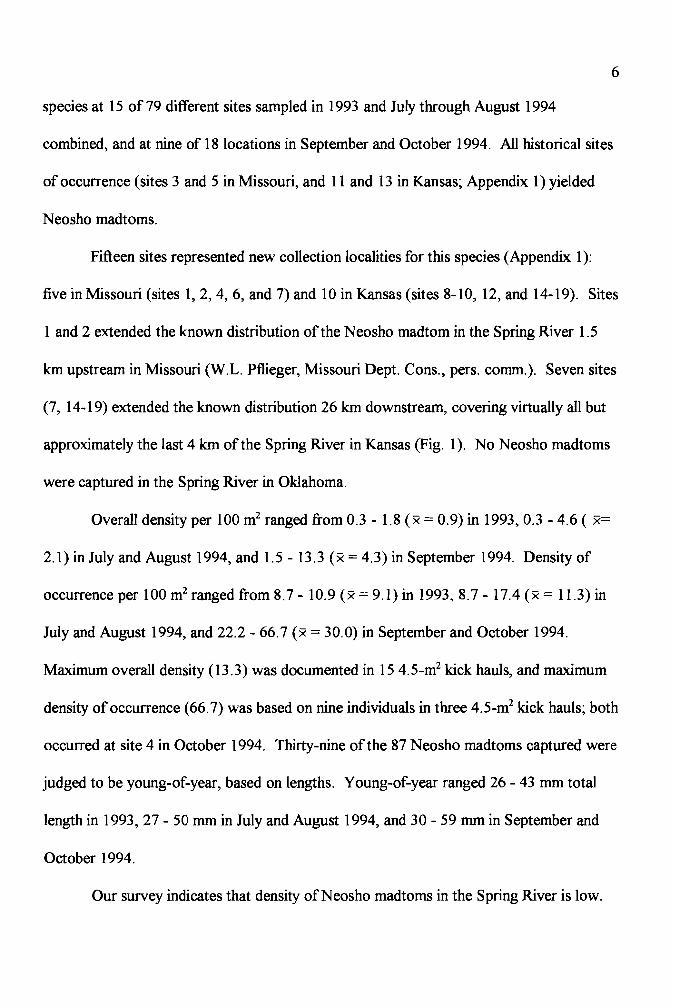
6

species at 15 of 79 different sites sampled in 1993 and July through August 1994

combined, and at nine of 18 locations in September and October 1994. All historical sites

of occurrence (sites 3 and 5 in Missouri, and 11 and 13 in Kansas; Appendix 1) yielded

Neosho madtoms.

Fifteen sites represented new collection localities for this species (Appendix 1):

five in Missouri (sites 1,2,4,6, and 7) and 10 in Kansas (sites 8-10, 12, and 14-19). Sites

1 and 2 extended the known distribution ofthe Neosho madtom in the Spring River 1.5

km upstream in Missouri (W.L. Pflieger, Missouri Dept. Cons., pers. comm.). Seven sites

(7, 14-19) extended the known distribution 26 km downstream, covering virtually all but

approximately the last 4 km ofthe Spring River in Kansas (Fig. 1). No Neosho madtoms

were captured in the Spring River in Oklahoma.

Overall density per 100 m2 ranged from 0.3 - 1.8 (x = 0.9) in 1993,0.3 - 4.6 ( x=

2.1) in July and August 1994, and 1.5 - 13.3 (x = 4.3) in September 1994. Density of

occurrence per 100 m2 ranged from 8.7- 10.9 (x = 9.1) in 1993,8.7 - 17.4 (x = 11.3) in

July and August 1994, and 22.2 - 66.7 (x = 30.0) in September and October 1994.

Maximum overall density (13.3) was documented in 15 4.5-m2 kick hauls, and maximum

density of occurrence (66.7) was based on nine individuals in three 4. 5-m2 kick hauls; both

occurred at site 4 in October 1994. Thirty-nine of the 87 Neosho madtoms captured were

judged to be young-of-year, based on lengths. Young-of-year ranged 26 - 43 mm total

length in 1993,27 - 50 mm in July and August 1994, and 30 - 59 mm in September and

October 1994.

Our survey indicates that density ofNeosho madtoms in the Spring River is low.

7

Their distribution in this river generally extended from downstream of the mouth of the

North Fork of Spring River in Jasper County, Missouri, through the area near the mouth

of Turkey Creek in Cherokee County, Kansas. Additionally, young-of-year Neosho

madtoms captured for the first time upstream from the mouth ofWillow Creek near

Baxter Springs, Kansas, (site 19) may represent an isolated population separated from

other Spring River collection localities by Empire Lake (Lowell Reservoir) and from

Neosho River populations by Lake 0' the Cherokees. The Neosho madtom has never been

documented from the Spring River in Oklahoma (USFWS, 1991~ Luttrell et al., 1992).

Collections ofNeosho madtoms at 15 new locations in the Spring River was likely

due, at least in part, to our intensive sampling effort over a 19-month period. Previous

surveys did not specifically examine the distribution and abundance of this species in the

Spring River. Lower mean densities in 1993 might have been the result of summer floods

which could have hampered Neosho madtom reproduction, recruitment, or both, and

might also have limited sampling effectiveness. Higher density estimates in the relatively

dry summer of 1994 could have been the result of river conditions that favored

recruitment, enhanced sampling effectiveness, or both. M. Eberle and W. Stark (Natural

Science Research Associates, Hays, Kansas), in a 1995 report to Kansas Department of

Wildlife and Parks, documented higher numbers ofNeosho madtoms in the Neosho and

Cottonwood rivers in 1994, compared to previous years, and suggested that higher

densities in 1994 might reflect improved habitat conditions due to freshly deposited, loose

gravel from 1993 floods. Though difficult to judge given the lack of sufficient previous

data for comparison, it is possible that low densities ofNeosho madtoms in the Spring

8

River in 1993 are the norm for that river (M. Eberle, pers. comm.).

Mean estimates ofdensities ofNeosho madtoms in the Spring River for both years

were lower than those reported from the Neosho and Cottonwood rivers by other

investigators. Moss (1983) recorded a mean density ofoccurrence of43.3/100 m2 and a

mean overall density of32.4/100 m2 from four night-time electroshocking samples at one

Neosho River riffle west ofErie, Kansas, sampled seasonally during 1975-76. Wenke et

al. (1992) documented a mean density of occurrence of 17.0/100 m2 and a mean overall

density of6.8/100 m2 in the Neosho and Cottonwood rivers in 1989-90. Fuselier and

Edds (1994) noted a mean density of occurrence of 15.5/100 m2 and a mean overall

density of3.3/100 m2 in the Cottonwood River in 1992-93. One exception was the mean

density of occurrence of 30.0/100 m2 for September and October 1994. This estimate was

made from a small area sampled in each kick-haul (4.5 m2), where the minimum density of

occurrence possible was 22.2/1 00 m2 (i.e., one fish per haul). Nevertheless, Neosho

madtom densities may typically be highest in fall, after young-of-year are added to the

population.

Though sample size, timing, and investigators differed among the studies noted

here, density ofNeosho madtoms in the Spring River appears to be less than elsewhere in

its range. Ongoing projects are directed at understanding why Neosho madtom numbers

differ between the Spring River and the Neosho and Cottonwood rivers. Continued

research into the effects of environmental factors on the density, distribution, relative

abundance, recruitment, and year-to-year variation ofthe disjunct Neosho madtom

population ofthe Spring River is vital to our understanding of this threatened species and

9

its eventual recovery.

Support for this research was provided by the Kansas Department ofWildlife and

Parks through USFWS Section 6 funds, an Emporia State University Faculty Research

and Creativity grant, the National Biological Service, the U.S. Fish and Wildlife Service,

and Region VII ofthe U.S. Environmental Protection Agency. A. Bissing, K. Brunson, 1.

Bryan, C. Charbaneau, 1. Criqui, F. Durbian, R. Ferguson, D. Hardesty, P. Heine, G.

Horak, P. Lovely, M. Legg, B. Mueller, D. Mulhern, M. Means, D. Munie, S. Olson, 1.

Pitt, B. Poulton, S. Ruessler, B. Schrage, 1. Sumner, V. Tabor, T. Thorn, R. Walton, D.

Whites, and D. Wright assisted with fieldwork or other aspects ofthe study. L. Fuselier

and M. Eberle made helpful suggestions that improved the manuscript. Thanks to

conservation agencies in Missouri, Kansas, Oklahoma, and to USFWS regions 2,3, and 6

for issuing collecting permits. Special thanks to landowners along the Spring River who

graciously allowed access to study sites.

10

Literature Cited

Fuselier, L., and D. Edds. 1994. Seasonal variation in habitat use by the Neosho madtom

(Teleostei: Ictaluridae: Noturus placidus). The Southwestern Naturalist 39:217-223.

Luttrell, G.R, RD. Larson, W.J. Stark, N.A Ashbaugh, AA Echelle, and AY. Zale.

1992. Status and distribution of the Neosho madtom (Noturus placidus) in Oklahoma.

Proceedings of the Oklahoma Academy of Science 72:5-6.

Moss, RE. 1983. Microhabitat selection in Neosho River riffles. Ph.D. dissert.,

University ofKansas, Lawrence.

Pflieger, W.L. 1971. A distributional study ofMissouri fishes. Museum ofNatural

History, University ofKansas 20:225-570.

Spruill, T.B. 1984. Assessment of water quality resources in the lead-zinc mined areas in

Cherokee County, Kansas, and adjacent areas. US. Geological Survey, Lawrence,

Kansas. Open File Report 84-439.

US. Fish and Wildlife Service. 1991. Neosho madtom recovery plan. US. Fish and

Wildlife Service, Denver, Colorado.

II

Wenke, T.L., M.E. Eberle, G.W. Ernsting, and W.J. Stark. 1992. Winter collections of

the Neosho madtom (Noturus placidus). The Southwestern Naturalist 37:330-333.

Wilkinson, C. and L. Fuselier. 1997. Neosho madtoms (Noturus placidus) in the South

Fork of the Cottonwood River: implications for management of the species. Transactions

of the Kansas Academy of Science 100: 162-165.

12

Appendix 1. Spring River Neosho madtom collection localities, with general and legal site

descriptions, and dates ofcollections.

Jasper Co., Missouri: Site 1) 0.4 km downstream from county bridge 2.5 km east

ofWaco; NE 1/4 Sec. 18, T29N, R33W; 10 and 12 August and 10 October 1994. Site 2)

0.4 km upstream from MO Hwy 171 bridge; SW 1/4 Sec. 18, T29N, R33W; 11 August

1994. Site 3) 0.2 km downstream from MO Hwy 171 bridge; NE 1/4 Sec. 24, T29N,

R34W and NW 1/4 Sec. 19, T29N, R33W; 11 August 1994. Site 4) 0.4 km upstream

from county bridge 2.8 km south of Waco; SW 1/4 Sec. 23, T29N, R34W; 9 August and

3 October 1994. Site 5) 0.2 km downstream from county bridge 2.8 km south ofWaco,

0.8 km east ofKS-MO state line; NW 1/4 Sec. 26, T29N, R34W; 8 August and 4 October

1994. Site 6) 2 km downstream from county bridge 2.8 km south ofWaco, 0.8 km east

ofKS-MO state line; NE 1/4 Sec. 35, T29N, R34W; 2 October 1994. Site 7) 5 km SW of

Carl Junction, just downstream from Center Creek confluence; SW 1/4 Sec. 14, T28N,

R34W; 15 August 1993.

Cherokee Co., Kansas: Site 8) 0.2 km downstream from KS-MO state line in

right channel of river; SE 1/4 Sec. 1, T33S, R25E; 26 July 1994. Site 9) 0.7 km

downstream from KS-MO state line in right channel of river; SE 1/4 Sec. 1, T33S, R25E;

27 July 1994. Site 10) 0.9 km downstream from KS-MO state line in right channel

of river; NW 1/4 and SW 1/4 Sec. 1, T33S, R25E; 20 July 1994. Site 11) 0.6 km

upstream from mouth of Cow Creek at bottom of island in both channels of river; SW 1/4

Sec. 1 and SE 1/4 Sec. 2, T33S, R25E; 5 September 1993 and 27-28 July 1994.

13

Site 12) 0.3 kIn upstream from KS Hwy 96 bridge; SW 1/4 Sec. 11, T33S, R25E; 4

September 1993 and 21 September 1994. Site 13) just upstream from KS Hwy 96 bridge;

SW 1/4 Sec. 11, T33S, R25E; 4 September 1993 and 19 July and 22 September 1994.

Site 14) 0.7 kIn downstream from KS Hwy 96 bridge in right channel of river; NE 1/4

Sec. 14, T33S, R25E; 3 August and 28 September 1994. Site 15) 1.4 kIn downstream

from KS Hwy 96 bridge in left split of river; SE 1/4 Sec. 14, T33 S, R25E; 3 August 1994.

Site 16) 2.3 kIn downstream from KS Hwy 96 bridge; NW 1/4 Sec. 24, T33S, R25E; 27

September 1994. Site 17) 1 kIn upstream from Turkey Creek confluence; SE 1/4 Sec. 25,

T33S, R25E; 5 September 1993. Site 18) immediately downstream from Turkey Creek

confluence; NW 1/4 Sec. 36, T33S, R25E; 6 September 1993. Site 19) 0.6 kIn upstream

from Willow Creek confluence in left channel of river; NE 1/4 Sec. 36, T34S, R24E; 6

October 1994.

Chapter 2

Spatial pattern and environmental correlates of the

Spring River basin fish assemblage

15

Abstract

We examined patterns of spatial heterogeneity in the Spring River basin fish

assemblage along with environmental correlates to assess the relative importance of

geographic distances and habitat differences among sites in explaining assemblage

structure. Mantel tests and Mantel correlograms indicated that fish species composition

and abundance were spatially autocorrelated and exhibited a patch size ofabout 44 km at

the basinwide scale. We used partial Mantel tests to remove the effects of spatial

autocorrelation from habitat variables before modeling habitat factors influencing fish

assemblage structure. Substrate particle size, mesohabitat type, nitrate, CO2, pH, stream

gradient, and stream size were significantly correlated to principal coordinate axes of

spatially-corrected environmental matrices. Space-constrained cluster analysis and

principal coordinates analysis revealed three primary groups of sites, reflecting relatively

distinct fish faunas within the Ozark, Lowland, and mainstream regions of the basin.

Within individual streams, longitudinal pattern was more apparent than it was at the

basinwide scale, and spatial autocorrelation of species and environmental differences were

of varying importance, consistent with the concept that stream systems act as mosaics of

interacting patches. Spatial patterns of the fish assemblage and environmental correlates

were consistent with a hypothesis ofvicariance biogeography as the primary organizing

factor, but a linkage between mainstream and tributary assemblages along with spatial

autocorrelation in species composition suggested contagious biotic processes are

important in maintaining assemblage structure, particularly at the interface between the

mainstream Spring River and its tributaries.

16

Introduction

Processes underlying spatial heterogeneity in stream communities include biotic

and abiotic factors which act together to influence community structure (power et al.

1988; Palmer and Poff 1997). Stream fish communities have primarily been characterized

as varying longitudinally along gradients of physical and chemical habitat variables (e.g.,

Schlosser 1987). Some researchers have recognized that movements by individuals are

important processes in structuring lotic communities (power et al. 1988; Freeman 1995)

and, in some cases, processes occurring downstream can affect communities upstream

(Osborne and Wiley 1992; Pringle 1997).

Recently ecologists have begun to emphasize the importance that spatial

autocorrelation, the similarity among variables based on the proximity ofcollecting sites to

one another, can have as a factor explaining the structure of communities (Legendre 1993;

Mandrak 1995; Cooper et al. 1997). Quantifying spatial pattern in communities can be

critical to identifying processes underlying community patterns (Sokal and Thomson

1987), and allows assessment of the relative importance of different hypotheses seeking to

explain observed heterogeneity (Douglas and Endler 1982; Burgman 1987; Mandrak

1995). In addition, spatial autocorrelation among data can lead to spurious correlations

between variables responding to a common underlying spatial pattern, and should be

removed from community response data before drawing inferences about processes

underlying the patterns (Legendre 1993; Mandrak 1995). Models of community structure

which include the influence of spatial autocorrelation are still in their early stages of

development (Legendre 1993), but statistical techniques designed to study autocorrelation

]7

among ecological data have allowed researchers to begin quantifYing spatial pattern in

communities. Quantification of spatial autocorrelation in stream communities provides a

way to identifY the scale at which patches exist and can be used to assess the importance

of spatial dependence in models of community structure (Cooper et al. ]997). However,

few studies have used autocorrelation techniques to examine spatial heterogeneity in

stream communities (but see Douglas and Endler 1982; Cooper et al. 1997).

The Spring River basin, situated in southwestern Missouri, southeastern Kansas,

and northeastern Oklahoma, provides an ideal system to study spatial pattern of fish

assemblage structure. The basin contains a diverse fish assemblage and is positioned

between two physiographic provinces: the Central Lowlands and the Ozark Plateaus

(Fig. ]; Davis and Schumacher 1992; Adamski et al. 1995), regions also known as the

Central Irregular Plains and Ozark Highlands ecoregions (Omernik 1987). Differences in

habitats between the two portions of the drainage presumably limit movement offishes

adapted to a specific set of physicochemical variables (Matthews 1987; Mayden ]987a;

1987b). However, movement by individuals within streams and their dispersal from

source areas to sink areas might be an important factor influencing fish species

composition at some locations, particularly near the mouths of tributaries (Gorman] 986;

Osborne and Wiley 1992). The goals ofthe current study were to describe spatial pattern

in the Spring River basin fish assemblage and to use this information to draw inferences

about the relative importance of abiotic and biotic factors in influencing assemblage

structure. Our specific objectives were to 1) quantifY spatial pattern offish assemblage

structure within the Spring River basin and identifY distances over which contagious biotic

18

processes such as reproduction, mortality, and movements of individuals might affect

assemblage structure, 2) assess the importance of spatial autocorrelation relative to

physicochemical differences influencing fish assemblage structure on the regional scale and

within individual streams, and 3) analyze patterns of species similarity to assess the

relationship between mainstream and tributary fish assemblages.

Materials and Methods

Study Site

The Spring River, part of the Arkansas River basin, fonns a border between the

Central Lowlands and Ozark Plateaus (Davis and Schumacher 1992; Adamski et al. 1995).

Tributaries draining the Central Lowlands region in the northern and western portions of

the Spring River basin (Fig. 1) are characterized by low gradients, poorly sustained base

flows, and substrates consisting of mud and silt with shale and sandstone gravel (Davis

and Schumacher 1992; Adamski et al. 1995). In contrast, tributaries flowing out of the

Ozark Plateaus in the southeastern portion of the basin (Fig. 1) have generally higher

gradients, sustained flows due to headwater springs, and substrates predominated by

limestone and chert gravel (Davis and Schumacher 1992; Adamski et al. 1995). Annual

precipitation averages 102 - 107 cm throughout the Spring River basin (Adamski et al.

1995), and altitude in the study site ranges from 223 m at the most downstream location

sampled in the Spring River mainstream to 451 m at the headwaters of Shoal Creek.

During our study we sampled North Fork of the Spring River, Cow Creek, Brush

Creek, and Willow Creek in the Central Lowlands region, and Center Creek, Shoal Creek,

19

Figure 1. Approximate distribution of sites where fish collections were made in the Spring

River basin during 1994-95.

20

ft° Central Ksl MO ARLowlands i

2217 0 : o16 0 1 23

13 0 o 24COW20 o :

1 oCk. 2 0 :21

o9zs North 2 I 37 36 51Q35Fork 34 50: 000 0

56 154 0 32 • R \ : 0 31 0 38 Sprmg . 25

Brush Ck... 18 \ 44 b0l6 0 0 0 39

o 15 ~ -h042 0 41 0o 19 0'-'43 45 6 40011 '7 0

oWillow Ck. 0 0 18 47 Center Ck. 0 0 0 00 0 0 7 8 33 0

12 10 9 o?~ 26 ... - .. _ .. _ .. _ .. _ .. _ .. _ .. - ~0?29 0 48 27 49

530 :1 30 0 00 • 14 5

is-mile Ck. 0 Shoal Ck. 0 3 Ozark , 01 4 Plateausi 00 I

OK:MO -10km

21

and Five-mile Creek in the Ozark region (Fig. 1). In addition we sampled the Spring

River mainstream which, upstream from its confluence with North Fork of the Spring

River, has characteristics of other Ozark streams (Davis and Schumacher 1992). At the

beginning of the study we recognized Ozark tributaries, Lowland tributaries, and the

mainstream Spring River, downstream from its confluence with North Fork of the Spring

River, as three distinct regions based on the well-documented physicochemical differences

between the Ozark and Lowland regions (Omernik 1987; Davis and Schumacher 1992;

Adamski et al. 1995), and our prediction that the mainstream Spring River would have a

distinct fish fauna because of its size and position within the drainage network.

Samplini

During spring and summer of 1994 and 1995, we collected fishes at 58 sites within

the Spring River basin (Fig. 1). Sites were selected primarily to fulfill our goal of

sampling representative streams from headwaters to tailwaters, including all stream orders.

We chose stream order (Strahler 1957) as an a priori criterion in site selection because it

allowed us to assess longitudinal patterns within individual streams. In some streams we

sampled more than one site in a reach of a particular order. Further criteria in site

selection were accessibility and landowner permission.

Fishes were collected by seining, performed during daylight hours with a 4.6-m by

1.8-m seine with 4.7-mm mesh. To assess relative abundance of fishes, standardized

sampling was conducted by three persons kick-seining and sweep-seining until all available

mesohabitats had been thoroughly sampled; in each sample we made approximately 25 to

22

35 seine hauls in a stream reach 100 to 300 m long, in 1.5 to 3 hours, depending on the

number of distinct habitats at each collection site. All fishes were identified and counted.

Protected species were released alive at their sites of capture following completion of

sampling at each location; voucher specimens ofnon-listed fishes were preserved for each

collection, and are housed in the Division ofBiological Sciences at Emporia State

University.

To assess habitat differences among sites as factors explaining differences in fish

species composition, we characterized each collecting site with 28 variables and used them

to construct four environmental matrices. One of us (CW) visually estimated percent

coverage of 15 physical habitat variables at each site to make the physical habitat matrix.

Substrate types, categorized according to a modified Wentworth scale, were mud, sand,

gravel, small cobble, large cobble, boulder, and bedrock. Other habitat variables were

mesohabitat type (i.e., riffle, run, pool, backwater), emergent vegetation, submergent

vegetation, canopy cover, and woody structure. For the water quality matrix we

measured dissolved oxygen, carbon dioxide, total alkalinity, hardness, nitrate, phosphate,

and pH with Hach water chemistry kits, as well as water temperature. In addition we

constructed an elevation matrix consisting of altitude and gradient, obtained from

topographic maps, and a stream size matrix consisting of drainage area, obtained from on­

screen digitizing ofUSGS 250K Digital Elevation Models using IDRISI for Windows

(version 1.01, Clark Labs, Worcester, MA), cross-sectional area, and maximum stream

width.

23

Statistical Analyses

Multivariate analyses used in measuring the influence of spatial autocorrelation

were conducted using the R-package for Macintosh computers (version 3.0, University of

Montreal, Montreal, Canada). Mantel tests (Mantel 1967; Sokal and Rohlf 1995) were

used to test for spatial autocorrelation in fish species data and to assess the importance of

environmental variables in influencing fish species composition. The Mantel test compares

two symmetric matrices of association by calculating a standardized Mantel statistic r,

equivalent to a Pearson product-moment correlation coefficient, between off-diagonal

elements of the matrices (Legendre and Vaudor 1991; Fortin and Gurevitch 1993; Sokal

and Rohlf 1995). Significance of correlations is assessed by randomly rearranging the

rows and columns of one of the matrices being compared, and constructing a null

distribution against which the initial Mantel r is compared. Mantel statistics significantly

larger than scores in the null distribution indicate a positive association between the two

matrices, whereas significantly smaller Mantel statistics indicate a negative association.

All Mantel and partial Mantel tests were conducted at a= 0.05, with Bonferroni

corrections in cases where multiple tests were conducted on the same matrices.

Significance was assessed using 5000 permutations for each test.

To analyze spatial pattern at the scale of the entire basin, we constructed a series

of 58 by 58, off-diagonal, symmetric matrices representing the geographic distances,

environmental variables, and fish species dissimilarities. In addition, subsets of these

matrices were used to assess factors influencing species composition within individual

streams of the basin; longitudinal spatial pattern within individual stream channels was

24

investigated by constructing dissimilarity matrices using all sites connected in a

unidirectional pathway between the headwaters of a stream and the most downstream site

in the Spring River mainstream. We did not separately analyze longitudinal pattern within

Brush, Willow, and Five-mile creeks because of the small number ofcollections made in

these streams.

Before analyzing fish species data we removed from the data set species occurring

in less than five percent ofcollections (Gauch 1982). We then constructed a fish species

dissimilarity matrix (hereafter the species matrix), comparing presence-absence of 59

species among all sites, using Jaccard's coefficient subtracted from unity (Marczewski­

Steinhaus distance: Pielou 1984). In addition, we investigated patterns of species

abundances by constructing a separate matrix ofEuclidean distances between sites based

on log (In(x+ 1)) transformed abundance data (hereafter the abundance matrix).

To construct the geographic distance matrix we used the Geographic Distances

program in the R-package to calculate the shortest straight-line distance between sites

based on their geographic coordinates. We concluded that this method of calculating

geographic distances was more appropriate than calculating distances along the stream

channel as preliminary investigation revealed that the correlation between stream-channel

distances and species dissimilarities was lower due to sites in adjacent streams that

contained similar species yet were very distant via the stream channel. We believe this

methodological concern is noteworthy because it reflects the important linkage between

streams and their terrestrial setting (e.g., Omernik 1987).

After testing the species presence-absence and abundance data for spatial

25

autocorrelation, we used Mantel correlograms (Legendre and Fortin 1989; Legendre

1993; Cooper et al. 1997) to describe the spatial pattern ofthe fish assemblage. In a

Mantel corre1ogram the geographic distance matrix is divided into a series ofbinary

matrices, each representing a distinct distance class interval, which are then compared

against a matrix representing associations among the variable of interest. Significance of

correlations in a Mantel correlogram is assessed using a Bonferroni-corrected error rate

(Legendre and Fortin 1989).

As a post hoc test of the importance of ecoregion in describing differences in

species composition among sites, we constructed a binary matrix consisting of zeroes to

characterize sites occurring in the same a priori predicted ecoregion, and ones to

characterize sites occurring in different ecoregions, then compared the resulting matrix

against the species matrix using a Mantel test. This technique is designed to assess

whether there is a greater difference within predetermined groups or among predetermined

groups, as a type ofnonparametric analysis ofvariance (Fortin and Gurevitch 1993, Sokal

and Rohlf 1995). Then, to determine the extent to which spatial autocorrelation among

species data was explained by differences among ecoregions, we conducted a partial

Mantel test comparing the species matrix against the geographic distance matrix while

holding the effects of the ecoregion matrix constant.

To investigate the species data for groups existing at the basinwide scale, we

conducted space-constrained cluster analysis (Legendre 1987; Legendre and Vaudor

1991; Legendre 1993) and principal coordinates analysis (PCoA) on the basinwide species

matrix. Legendre (1987) explains that space-constrained cluster analysis is appropriate for

--

26

identifying groups within spatially autocorrelated data because it incorporates the spatial

structure into the analysis. The technique uses a proportional-link clustering algorithm as

in other clustering techniques, but restricts clustering to sites adjacent to one another

(Legendre and Vaudor 1991). PCoA allowed us to validate species groups identified by

cluster analysis. Before cluster analysis, we chose 20% as the connectedness level for the

clustering algorithm (Legendre 1987; Legendre and Vaudor 1991), and determined

linkage of sites using a Delaunay triangulation. In triangulation, three points (i.e.,

collecting sites) are considered linked if the circle passing through the three points fails to

encompass any other points under study (Legendre and Vaudor 1991). We modified the

triangulation by adding two links between sites adjacent along stream channels, thus

allowing potential movement of fishes between sites, but not identified as linked by

triangulation. Sokal and Oden (1978) present a case in which they make a similar

modification to a linkage network.

To assess correlations among the species, geographic distance, and environmental

data sets we constructed environmental matrices by calculating Euclidean distances

between all pairwise combinations of sites, and compared matrices using Mantel tests.

Before constructing environmental matrices we arcsine transfonned percentage data in the

physical habitat matrix (Sokal and Rohlf 1995) and, except for pH, In(x+1) transfonned

values in the elevation, stream size, and water quality matrices, to standardize and

nonnalize variables. To identify gradients which might have influenced assemblage

structure we conducted PCoA on environmental matrices. For environmental matrices

identified as spatially autocorrelated, we used partial Mantel tests to remove the influence

27

of common spatial structure in the environmental and species data sets (Smouse et al.

1986; Mandrak: 1995) before subjecting the spatially corrected matrices to PCoA

(Mandrak: 1995). We then calculated bivariate correlations between environmental

variables and principal coordinate axes to determine axis loadings.

In addition to identifying gradients in the environmental data, we used PCoA to

determine whether sites that formed groups in cluster analysis grouped together in

ordinations of their environmental characteristics. In these analyses, and in PCoA of the

species matrix, we used uncorrected environmental matrices because our goal was to

describe the spatial pattern of variables without assuming environmental control of

assemblage structure (Legendre 1993).

Results

The Mantel test comparing the species and geographic distance matrices indicated

spatial autocorrelation among fish species presence-absence data (r=O.58,p=O.0002;

Table 1). The corresponding Mantel correlogram (Fig. 2) indicated positive

autocorrelation among the smallest distance classes and negative autocorrelation among

the largest classes, reflecting a pattern which can either be interpreted as describing

species distributed along a gradient, or with a sharp step between two relatively

homogenous taxonomic zones (Legendre and Fortin 1989). Significant positive

correlations for each of the four smallest distance classes indicated a zone of influence of

approximately 44 km within which fish collections tended to have a more similar species

composition than expected by chance. The species abundance data were also spatially

28

Table 1. Mantel correlations for comparisons between geographic distance, species

presence-absence, and environmental matrices. Number of coUections used for each site

group in parentheses. Above the diagonal: results ofMantel tests. Below the diagonal:

results of partial Mantel tests for autocorrelated data sets. Significance assessed using

Bonferroni-corrected error rate, a'=0.05/25 (25 possible comparisons for each site group)

= 0.002. Probability based on 5000 permutations, *p<0.002, **p=0.0002.

Site group Matrix 1. Species 2. Physical 3. Water 4. Elevation 5. Size

Habitat Quality

All (n=58) Distance 0.58** 0.14** 0.33** 0.22** -0.08

1. - 0.39** 0.41** 0.26** 0.14**

2. 0.36** - 0.50** 0.10 0.10

3. 0.29** 0.47** - 0.04 0.15**

4. 0.16** 0.07** -0.04 - 0.38**

5.

Spring R. (n=15) Distance 0.83** -0.006 0.14 0.57** 0.83**

1. - 0.08 0.28 0.35* 0.61 **

2. - -0.036 -0.14 -0.16

3. - -0.12 0.10

4. -0.26 - 0.69**

5. -0.23

North Frk. (n=17) Distance 0.65** -0.004 -0.04 0.38** 0.68**

1. - 0.43** 0.36** 0.36** 0.62**

2. - 0.38** 0.34* 0.24

3. - -0.03 -0.004

4. 0.16 - 0.85**

5. 0.31*

29

Table 1 cont.

Shoal Ck. (n=12) Distance 0.69** 0.16 0.22 0.83** 0.93**

I. - 0.71** 0.66** 0.69** 0.74**

2. - 0.78** 0.24 0.28

3. - 0.35 0.44*

4. 0.30 - 0.80**

5. 0.34

Center Ck. (n=12) Distance 0.58** 0.009 0.34 0.88** 0.83**

I. - 0.21 0.34 0.60** 0.69**

2. - -0.32 0.01 0.03

3. - 0.61 ** 0.56*

4. 0.23 - 0.76**

5. 0.46*

Cow Ck. (n=12) Distance 0.57** -0.3 I 0.62** 0.78** 0.85**

I. - -0.09 0.76** 0.71 ** 0.70**

2. - -0.3 I -0.33 -0.05

3. 0.62** - 0.85** 0.56**

4. 0.5 I ** - 0.70**

5. 0.50**

30

Figure 2. Mantel correlogram comparing spatial pattern of species presence-absence and

abundance data. Significance of correlations assessed using a Bonferoni-corrected error

rate, a' = 0.05110 (10 distance classes) = 0.005. Significant positive correlations above

the upper line, significant negative correlations below the lower line.

31

0.3

0.2

1i 0.1 jI, =0""",

CO' ~ 1

co I .. ~ ..A ~ -. L . ..-0.1'\:\

-C.3 '.... 02 1

/ / ..'

11 22 33 44 55 66 77 88 99 110 Distance class upper limit (km)

-­ presence-absence abundance

32

autocorrelated (r=0.42, p=0.0002) and exhibited roughly the same pattern (Fig. 2), with

positive autocorrelation among smaller, and negative autocorrelation among larger

distance classes. However, the 99 and 110 kIn distance classes were not significantly

autocorrelated (Fig. 2), possibly reflecting both the relatively small number of samples in

these distance classes (47 and 26 site-pairs, respectively) and the weaker overall

association between species abundances and geographic distances, compared with that of

species presence-absence.

Comparisons between the geographic distance matrix and each environmental

matrix indicated spatial autocorrelation among variables in the physical, water quality, and

elevation matrices, but not the stream size matrix (Table 1). Correlograms of

autocorrelated environmental data exhibited different spatial patterns at the basinwide

scale, which we interpret here following Legendre and Fortin (1989). Peaks in the

correlogram of the physical habitat matrix, reflecting positive autocorrelation of the 22

and 55 kIn distance classes, contrasted with significant negative autocorrelation of the 77

and 88 kIn distance classes (Fig. 3), suggest that these data were distributed in a patchy

spatial pattern. Water quality data appeared to be distributed as a gradient or a sharp step,

similar to the distribution of the species data, but with a 33 kIn zone of influence.

Elevation exhibited a patchy distribution with a patch size of33 kIn and a sharp trough of

negative autocorrelation over the 77 kIn distance class.

There was a relatively weak but significant correlation (r=0.I5, p=0. 0002) between

the binary ecoregion matrix and the geographic distance matrix, suggesting that although

differences among ecoregions explained some of the observed spatial autocorrelation

33

Figure 3. Mantel correlogram comparing spatial pattern of species presence-absence data

and spatially autocorrelated environmental variables. Significance of correlations assessed

using a Bonferoni-corrected error rate, a. ' = 0.05110 (10 distance classes) = 0.005.

Significant positive correlations above the upper line, significant negative correlations

below the lower line.

34

0.3 1

02 1,

-------' • ~I .._".............. " ,I "..

~ 0.1 I /'s-..:::.:... :::.::-.._ ~. - '7 ~ ..,.~m - ~-- or .~ ,..,).... .. . c I " :.:..~.../

~ ,,~ ..... ~ ,0::::::; -0 1 ". \<.~ '"

· I '<\ ) ..:... ·,.._..-.. r "'~.~--02 ..... /

• "~'..f..... ,/ ...... -..... -.....,/L-0.3

11 22 33 44 55 66 77 88 99 110 Distance class upper limit (km)

species physical habitat elevation water quality

35

among species, there was additional spatial dependence that could not be explained by

these differences. Results of the partial Mantel test between the species and geographic

distance matrices, holding the effects of ecoregion constant, indicated further spatial

structure in the species data besides that influenced by ecoregions (r=O.57,p=O.0002).

Because spatial structure of the species data was better represented in the species

matrix than in the abundance matrix, the remaining analyses were conducted using

presence-absence data. Results ofMantel tests indicated significant correlations between

the species matrix and each of the environmental matrices (Table 1). After partialling out

the influence of common spatial structure from the data sets, the physical, water quality,

and elevation matrices remained significantly correlated to species dissimilarities (Table 1),

suggesting that variables in these matrices, as well as variables in the stream size matrix,

may have been important in structuring the fish assemblage. However, significant

correlations between some environmental matrices led us to believe that covariation

among variables in these matrices might have resulted in spurious correlations between the

species and environmental matrices (Table 1). To address this potential problem we

conducted partial Mantel tests to compare environmental matrices with the species matrix

while holding the effect of the covariable matrix constant. Because correlations between

environmental and species matrices remained significant after removing the influence of

covariates, we subjected all four matrices to PCoA (i.e., spatially-corrected physical, water

quality, and elevation matrices, and the uncorrected size matrix).

The amount ofvariation explained by the first two PCoA axes for each data set

was small. The first two axes of the spatially-corrected physical habitat PCoA accounted

36

for only 6.2% of the total variation in the data set. PCoA 1 (3.6%) contrasted sites where

mud substrate and pool mesohabitat were prevalent, with sites characterized by gravel,

small cobble, riffles, and runs (Table 2). Similarly, PCoA 2 of physical habitat (2.6%)

contrasted sites dominated by gravel and small cobble with sites characterized by mud and

bedrock (Table 2). The first two PCoA axes of the spatially-corrected water quality

matrix explained 6.8% of the total variation in the data set; PCoA 1 explained 4.4% and

was correlated most highly with gradients of nitrate, CO2, and pH (Table 2). The first and

second axes of the spatially-corrected elevation matrix explained 3.4% and 2.1 % of the

total variation among sites, respectively. Gradient had higher correlations with the first

and second axes than did altitude, and both variables were significantly correlated with

PCoA 1 (Table 2). The first two principal coordinate axes of the uncorrected stream size

matrix explained 10.2% of the variation in the data set. Drainage area, cross-sectional

area, and maximum width were correlated with the first axis (6.6%), and cross-sectional

area was significantly correlated with PCoA 2 (Table 2).

Comparing subsets of the geographic distance and species matrices indicated

significant spatial autocorrelation of species within all streams tested (Table 1).

Physicochemical differences were ofvariable importance in explaining species differences

at sites within individual streams, as indicated by significant correlations between species

dissimilarities and physical habitat and water quality differences in some instances, but not

others (Table 1). Elevation and stream size matrices were significantly correlated with

species dissimilarities in all streams tested; however, when the effects of spatial

autocorrelation were removed from these data sets using partial Mantel tests, correlations

37

Table 2. Bivariate correlations between variables in environmental matrices and the first

two PCoA axes of spatially-corrected physical habitat, water quality, and elevation

matrices, and uncorrected stream size matrix. Significance of correlations assessed using

Bonferroni-corrected error rate, a' = 0.05/28 = 0.0018, *p < 0.0018, **p < 0.001.

PCoA 1 PCoA2

Physical habitat (variation explained) 3.6% 2.6%

riflle 0.44* 0.26

run 0.60** 0.07

pool -0.87** -0.25

backwater 0.27 0.31

mud -0.67** -0.44*

sand -0.08 -0.23

gravel 0.42* 0.66**

small cobble 0.45** 0.56**

large cobble 0.41 0.32

boulder 0.11 -0.08

bedrock 0.22 -0.42*

canopy -0.18 -0.18

submergent vegetation -0.01 -0.31

emergent vegetation -0.01 0.19

woody structure -0.14 -0.18

38

Table 2 cont.

Water quality (variation explained) 4.4% 2.4%

dissolved oxygen -0.37 0.03

carbon dioxide -0.76* 0.05

total alkalinity -0.38 0.13

hardness 0.11 -0.08

nitrate -0.78* -0.01

phosphate -0.23 0.04

temperature -0.37 0.22

pH -0.73* 0.32

Elevation (variation explained) 3.4% 2.1%

altitude 0.65** 0.07

gradient 0.94** 0.23

Stream size (variation explained) 6.6% 3.6%

drainage area -0.94** -0.29

cross-sectional area -0.84** 0.70**

maximum width -0.82** -0.19

39

between stream size and species differences remained significant only in North Fork of the

Spring River, Center Creek and Cow Creek, while the correlation between elevation and

species differences remained significant only in Cow Creek (Table 1). Higher correlations

in individual streams, compared with correlation between the complete data sets,

demonstrate that analyzing spatial autocorrelation at the basinwide scale does not

completely account for longitudinal patterns present within streams.

Cluster analysis of the overall species matrix identified three groups (Table 3)

which fit closely to the groups based on ecoregions predicted a priori. Exceptions were

two Ozark sites (4 and 8), eliminated from the analysis because they were outliers which

would have prevented the fusion of their neighboring groups (Legendre 1987), and seven

sites (bold in Table 3) located at the downstream positions in tributaries, adjacent to

mainstream locations. Mainstream fish collections, forming a cluster along with these

seven downstream tributary sites, were characterized by Pimephales notatus, Notropis

rubel/us, Labidesthes sicculus, Lepomis macrochirus, and Percina copelandi (Appendix

1) as the most frequently occurring species. Collections in Ozark tributaries tended to

cluster together (Ozark group, Table 3), except for sites in the most downstream positions

in Shoal Creek, Center Creek, and the Spring River headwater upstream from its

confluence with North Fork of the Spring River, which were more similar to mainstream

collections. The most frequently occurring species in the Ozark group were Campostoma

anomalum, Luxilus cardinalis, N rubel/us, Cottus carolinae, and Etheostoma spectabile

(Appendix 1). Similarly, Lowland tributary collections clustered together (Lowland

group, Table 3), except for three sites in North Fork ofthe Spring River, and the most

40

Table 3. Groups of sites identified by space-constrained cluster analysis using modified

triangulation to assess linkage among sites (connectedness = 0.20, clustering level = 0.33).

Site numbers refer to collection localities designated in Figure 1. Numbers in bold

distinguish tributary and Spring River headwater sites that clustered with collections from

mainstream sites.

31

55

11

54

Mainstream group

32

56

36

57

37

58

42 43 44 46 51 53

1

33

Ozark group

3

38

5

39

6

40

7

41

14

45

25

47

26

48

27

49

29

50

30

Lowland group

9

22

2

21

10

23

12

24

13

28

15

34

16

35

17

52

18 19 20

41

downstream site in Brush Creek, all ofwhich clustered with mainstream collections. The

most frequently occurring species in the Lowland group were Lythrurus umbratilis,

Gambusia affinis, Lepomis cyanellus, L. macrochirus, and Micropterus salmoides

(Appendix 1).

PCoA of the uncorrected species matrix (Fig. 4) for the most part corroborated

species groups identified in space-constrained cluster analysis. PCoA 1 (20.0%) described

a contrast between Ozark and Lowland collections, with mainstream sites between and

overlapping the other groups. PCoA 2 (13.7%) further distinguished most sites belonging

to the Mainstream species cluster from those in the Ozark and Lowland groups. Sites

positioned at the interface between Mainstream and Lowland groups included 11 and 55,

which grouped with Mainstream sites in cluster analysis, as well as site 52, which grouped

with Lowland sites (Table 3). In addition, site 11 in Brush Creek and site 51 in North

Fork ofthe Spring River (Fig. 1) did not group together with other mainstream sites in

PCoA of uncorrected physical habitat and water quality matrices (Fig. 5), suggesting that

these sites had different habitat characteristics than other Mainstream sites despite having

species compositions which included "mainstream species."

42

Figure 4. Plot ofthe first and second principal coordinate axes offish species

dissimilarity. Symbols represent groups of sites which clustered together in space­

constrained cluster analysis identified in Table 3; crosses = Mainstream, triangles =

Lowland, circles = Ozark

(%O'OZ) ~ VO~d

9'0 Z'O 0 17'0­,--------------~---------~ 9'0­

•'.•• . •

•• )jJezQ

++ weaJlSu!e~ t~ +

L ----=t='-------------L..... 17'0

tV

44

Figure 5. Plot of the first and second principal coordinate axes ofuncorrected (a) physical

habitat and (b) water quality matrices. Symbols represent groups of sites which clustered

together in space-constrained cluster analysis (Table 3); crosses = Mainstream, triangles =

Lowland, circles = Ozark.

45

100

A80 f-Uncorrected 11 Physical Habitat + 5160 +- A A

~ 40 0) A

e A AA20N A -tr..- + +

A ~ 0 A ••A

Q.. A • +

u A~ • • +4I!t....~. -20 + +

• +A• + +.-40f- +

A I I I I I-60 I

-100 -80 -60 -40 -20 0 20 40

PCoA 1 (15.1%) (a)

1.5 -,- -------a I I

Uncorrected1 I A Water Quality

A

;e 0.5 0 Cl ci- 0N c(

8c.-0.5

+ + .-... + * •~,Jt A+.

• A A#.

• • ~

A

A A

51

A

11 +

A AA

A A A A

-1 J--­ • +• •

-1.5 ---r-­-1 -0.5 0 0.5 1 1.5 2

PCoA 1 (37.4%)

(b)

46

Discussion

Studies of community structure indicate that abiotic and biotic influencing factors

are not mutually exclusive (Borcard et al. 1992), and assemblage structure in stream

systems responds to a combination offactors (Schoener 1987; Power et al. 1988).

Whereas correlational studies cannot conclusively identify causative mechanisms

responsible for ecological patterns, describing and quantifying spatial pattern in

communities can lead to a better understanding of the relative importance ofprocesses

which act to create the observed patterns.

The spatial pattern of the Spring River basin fish assemblage comes as no surprise

considering the distinctive fish faunas ofthe Ozark HigWands and Central Lowlands

(Mayden 1987a; 1987b). Distributional patterns of fishes in the Spring River basin,

together with the geological history of the region, are consistent with vicariance

biogeography as the primary process underlying present structure of the basinwide fish

assemblage (Mayden 1987a; 1987b). In this scenario, the Arkansas River separated the

Ozark Plateaus from the Ouachita Mountains and made habitats in the intervening region

more like the adjacent Central Lowlands (Mayden 1987b). Thus, the close fit between

species clusters and physiographic provinces supports the applicability of ecoregions as a

means ofdescribing biotic assemblages (Hughes et al. 1987; Edds 1993; Lyons 1996). In

addition, the distributional pattern of the fish assemblage, identified by Mantel

correlograms, reflects the distinction between the Lowland and Ozark portions of the

drainage, and the distance between most sites of each region falls within the 44 km zone of

influence, or patch size. However, the three groups of sites identified by PCoA and space­

47

constrained cluster analysis reflect not only disparate fish faunas of the two biogeographic

provinces in the basin, but a distinct fish fauna in the Spring River mainstream as well.

Though environmental and species differences in our study were significantly

correlated, the small proportion of species variation explained by environmental

differences (Table 1) suggests that other factors were important in organizing the

community as well. Further, physical habitat variables we measured exhibited a patchy

distribution not closely matching the pattern exhibited by the assemblage (Fig. 3). This

suggests that mesohabitat type and substrate size, factors significantly correlated to

physical habitat PCoA axes (Table 2), might have a more localized than regional influence

in the Spring River basin. Considering the congruence between species clusters and

ecoregions, other factors that differ between regions, such as soil type and stream

productivity (Omernik 1987~ Lyons 1996), or stream flow variability (Poffand Allan

1995~ Taylor et al. 1996) might have further accounted for observed species differences at

the basinwide scale. However, the high degree of spatial autocorrelation which remained

among species after partialling out the effect of ecoregions suggests that other factors,

besides those encompassed in ecoregions, were responsible for the observed community

structure.

Autocorrelation analysis offers circumstantial evidence that contagious biotic

processes may also explain variation in the species assemblage not explained by

environmental differences among sites. In the overall analysis and in most individual

streams of the basin, spatial autocorrelation explained more of the variation in species

composition than did habitat differences (Table 1). For instance, spatial analysis of

48

longitudinal pattern in the Spring River (Table 1) indicated that distance between sites

accounted for 69% (coefficient of determination =r = 0.832 = 0.69) of the variation in

species, whereas none of the environmental matrices were significantly correlated to

species differences after the influence of spatial autocorrelation was removed (Table 1).

Partial Mantel tests helped reveal several spurious correlations between species

and environmental matrices that were the result of common spatial structure among

variables in those data sets. Particularly within individual stream channels, positive

correlations between species differences and both the elevation and stream size matrices

gave the false impression that variables in these matrices accounted for a high degree of

variation in species composition, when spatial autocorrelation among sites explained more

of the variation. The usefulness ofelevation as an explanatory variable for aquatic

community structure has been questioned by some researchers who consider it a surrogate

for other environmental factors such as stream hydraulics (Statzner and Rigler 1986).

Similarly, stream size may be a surrogate for habitat complexity (Gorman and Karr 1978;

Schlosser 1987) or stability (Schlosser 1987). Though our attempt to model factors

important in structuring the Spring River basin fish assemblage was not intended to be

exhaustive, these results suggest that much of the influence attributed to environmental

differences can be alternatively explained by the spatial pattern underlying the data.

The influence that processes occurring downstream can have on the biota of

upstream reaches in some drainage networks has recently been emphasized by ecologists

who have recognized that the familar upstream-downstream linkage described in the River

Continuum Concept (Vannote et al. 1980; Minshall et al. 1985) is an oversimplification of

49

the processes affecting assemblage structure (Osborne and Wiley 1992; Pringle 1997).

For fishes in the Spring River basin, groups of sites identified by cluster analysis reflect the

influence of the mainstream fish assemblage on species composition in tributaries, in that

sites in downstream positions of some tributaries were occupied by species more

characteristic of the mainstream fish assemblage than of adjacent tributary collections. For

example, Cyprinella spiloptera was collected from the most downstream sites in North

Fork of the Spring River (sites 36 and 37), Brush Creek (site 11), Center Creek (site 42),

and Shoal Creek (site 58), but not at any other tributary site. Other species primarily

occurring in mainstream collections and downstream tributary sites were Notropis

volucellus, Cyprinella camura, Pimephales tene/lus, P. vigilax, Ietalurns punctatus,

Percina phoxocephala, and P. copelandi. The presence of "mainstream species" in

tributaries was not restricted to tributary collections that grouped with mainstream

collections in cluster analysis, as exemplified by the most downstream site in Cow Creek

(52), which clustered with other Lowland tributary sites, but contained species such as P.

tene/lus, P. vigilax, 1. punctatus and P. phoxocephala. Although the fish assemblage at

this site had a higher proportion of species present at adjacent tributary sites than at

adjacent mainstream sites, the presence of "mainstream species" provides evidence of a

linkage between the mainstream and Cow Creek not apparent in the cluster analysis.

Another characteristic of the basinwide fish assemblage that cluster analysis did not

adequately assess is the longitudinal pattern of fishes and environmental correlates in

individual streams of the basin. The importance of longitudinal patterns was somewhat

reflected in PCoA of the basinwide species matrix, however, with larger tributary reaches

50

located nearer to, and in some cases overlapping, the mainstream group (Fig. 4). Using

autocorrelation techniques to analyze patterns in individual streams, in some cases,

revealed substantial longitudinal gradients. These gradients were not apparent in the

basinwide analysis which compared sites in adjacent streams and thus tended to favor

regional patterns. This distinction may be partially a matter of scale, in that longitudinal

distribution in streams appears to be more important on a local scale than on a regional

scale, possibly as a reflection of processes, such as predation and competition, which act at

a local scale, versus historical biogeography and differences in stream productivity, which

act at a regional scale. The varying importance of geographic distance and habitat

differences as variables explaining species composition at sites within different streams

may reflect differences among streams in the processes acting to structure fish

assemblages (Table 1). In addition, the differing degrees of spatial autocorrelation

exhibited by fish assemblages in individual streams compared to the entire basin supports

the idea that stream systems function as "mosaics of patches" (Pringle et al. 1988).

Though our analysis cannot distinguish between fish movements and other

contagious processes such as reproduction and mortality, movements of individuals are

known to be important controlling processes in stream systems (Power et al. 1988). At

least two species characteristic of mainstream Spring River collections have been reported

to seasonally migrate into tributaries to reproduce, C. spiloptera (Gorman 1986) and 1.

punctatus (Dames et al. 1989). Migration of fishes presumably requires certain habitat

patches to be present along the migratory pathway (Pringle et al. 1988), so it is not

surprising that PCoA (Fig. 5) reflected the similarity among habitat characteristics at sites

51

belonging to the Mainstream species group. However, the fact that sites 11 and 51 in the

downstream portions of two tributaries were distinguished from mainstream sites based on

ordination of physical habitat and water quality differences suggests that the linkage

between mainstream and tributary species assemblages is capable of transcending

boundaries of habitat patches. This possibility is further reflected in the greater patch size

of the species assemblage compared with patch sizes ofhabitat variables (Fig. 3).

It is possible that the observed linkage between the mainstream and its tributaries is

only exhibited during part of the year when individuals are reproductively active and

"mainstream species" migrate into the tributaries. However, we do not believe this is the

case because, in Kansas, some of the species characteristic ofthe Mainstream group,

including P. copelandi and P. phoxocephala, spawn earlier in the year (Cross 1967) than

when we made our collections. In addition, all the species in the Mainstream group have

been collected in the downstream reaches of tributaries during other times of the year as

well (Branson et al. 1969). Rather, we believe it is plausible to view the mainstream­

tributary interface as a patch boundary which changes its location in response to dynamic

biotic interactions and bi-directional contagious processes. One manner in which changes

at the mainstream-tributary interface appear to be brought about is through disturbances,

such as those resulting from dams, in the lower portions of drainage networks (Pringle

1997). Using autocorrelation techniques to assess temporal changes in spatial pattern at

local and regional scales, together with manipulative experiments, might lead to additional

understanding of how these processes affect the perceived linkage between tributary and

mainstream assemblages.

52

Autocorrelation techniques used here are just a few of the multivariate and

univariate analyses designed to deal with spatially explicit data (e.g., Legendre and Fortin

1989, Legendre 1993, Ver Hoef and Cressie 1993, Fortin and Gurevitch 1993, Cooper et

al. 1997). Hopefully, stream ecologists will become more aware of the influence that

spatial autocorrelation can have in testing significance ofcorrelations used in models of

community structure, and will consider its influence before interpreting the results of

statistical tests on spatially autocorrelated data. Additionally, spatial autocorrelation can

be interpreted as a reflection of the relative importance ofbiotic processes in structuring

lotic communities, a factor that might otherwise be overlooked in community analyses. In

the future, if more stream ecologists incorporate spatial pattern as a factor in studies of

community ecology, models of patch dynamics will become more sophisticated, leading to

a better understanding of the causes and effects of spatial heterogeneity in streams.

Acknowledgments

Advice on statistical analyses was provided by N. Mandrak and L. Scott, and J.

Osborn reviewed the manuscript. Field collections were assisted by M. Combes, J. Criqui,

and J. Bryan, and fish enumeration was assisted by P. Bixel, C. True, D. Riedle, K.

Mitchell, and C. Hase. Assistance with data entry was provided by J. Kerr, and B.

Obermeyer aided retrieval of information from digital elevation maps. Special thanks to

landowners for allowing access to their property. Collecting permits were issued by

Kansas Department of Wildlife and Parks, Missouri Department ofConservation,

Oklahoma Department ofWildlife Conservation and U.S. Fish and Wildlife regions 2,3,

53

and 6. Financial support was provided by Kansas Department ofWildlife and Parks, U.S.

Fish and Wildlife Service, and an Emporia State University Faculty Research and

Creativity grant.

54

Literature Cited

Adamski, le., lC. Petersen, D.A. Freiwald, and lV. Davis. 1995. Environmental and

hydrologic setting of the Ozark Plateaus study unit, Arkansas, Kansas, Missouri, and

Oklahoma. United States Geological Survey, Water-Resources Investigations Report 94­

4022, Little Rock, Arkansas.

Borcard, D., P. Legendre, and P. Drapeau. 1992. Partialling out the spatial component of

ecological variation. Ecology 73: 1045-1055.

Branson, B.A., l Triplett, and R. Hartmann. 1969. A partial biological survey of the

Spring River drainage in Kansas, Oklahoma, and Missouri. Part II: the fishes.

Transactions of the Kansas Academy of Science 72:429-472.

Burgman, M.A. 1987. An analysis of the distribution of plants on granite outcrops in

southern Western Australia using Mantel tests. Vegetatio 71:79-86.

Cooper, S.D., L. Barmuta, O. Samelle, K. Kratz, and S. Diehl. 1997. Quanitfying spatial

heterogeneity in streams. Journal of the North American Benthological Society 16: 174­

188.

Cross, F.B. 1967. Handbook offishes ofKansas. Miscellaneous Publication no. 45,

University ofKansas Museum ofNatural History, Lawrence.

55

Dames, H.R. and T.G. Coon. 1989. Movements of channel and flathead catfish between

the Missouri River and a tributary, Perche Creek. Transactions of the American Fisheries

Society 118:670-679.

Davis, 1.v. and 1.G. Schumacher. 1992. Water-quality characterization of the Spring

River basin, southwestern Missouri and southeastern Kansas. United States Geological

Survey, Water-Resources Investigations Report 90-4176, Rolla, Missouri.

Douglas, M.E. and 1.A. Endler. 1982. Quantitative matrix comparisons in ecological and

evolutionary investigations. Journal ofTheoretical Biology 99:777-795.

Edds, D.R. Fish assemblage structure and environmental correlates in Nepal's Gandaki

River. Copeia 1993:48-60.

Fortin, M.-1. and 1. Gurevitch. 1993. Mantel tests: spatial structure in field experiments.

Pages 342-359 in S.M. Scheiner and 1. Gurevitch (editors). Design and analysis of

ecological experiments. Chapman and Hall, New York.

Freeman, M.C. 1995. Movements by two small fishes in a large stream. Copeia 1995:

361-367.

56

Gauch, H.G., Jr. 1982. Multivariate analysis in community ecology. Cambridge

University Press, Cambridge.

Gorman,O.T. 1986. Assemblage organization of stream fishes: the effect ofrivers on

adventitious streams. American Naturalist 128:611-615.

Gorman, O.T. and J.R. Karr. 1978. Habitat structure and stream fish communities.

Ecology 59:507-515.

Hughes, R.M., E. Rexstad, and c.E. Bond. 1987. The relationship of aquatic ecoregions,

river basins, and physiographic provinces to the ichthyogeographic regions of Oregon.

Copeia 1987:423-432.

Legendre, P. 1987. Constrained clustering. Pages 289-307 in P. Legendre and L.

Legendre (editors). Developments in numerical ecology. NATO ASI Series, Volume G

14. Springer-Verlag, Berlin.

Legendre, P. 1993. Spatial autocorrelation: trouble or new paradigm? Ecology 74: 1659­

1673.

Legendre, P. and M. -1. Fortin. 1989. Spatial pattern and ecological analysis. Vegetatio

80: 107-138.

57

Legendre, P. and A. Vaudor. 1991. The R package: multidimensional analysis, spatial

analysis. Departement de Sciences biologiques, Universite de Montreal.

Lyons,1. 1996. Patterns in the species composition offish assemblages among Wisconsin

streams. Environmental Biology ofFishes 45:329-341.

Mandrak, N.E. 1995. Biogeographic patterns offish species richness in Ontario lakes in

relation to historical and environmental factors. Canadian Journal ofFisheries and Aquatic

Science 52: 1462-1474.

Mantel, N. 1967. The detection of disease clustering and a generalized regression

approach. Cancer Research 27:209-220.

Matthews, W.1. 1987. Physicochemical tolerance and selectivity of stream fishes as

related to their geographic ranges and local distributions. Pages 111-120 in W.1.

Matthews and D.e. Heins (editors). Community and evolutionary ecology ofNorth

American stream fishes. University of Oklahoma Press, Norman.

Mayden, RL. 1987a. Pleistocene glaciation and historical biogeography ofNorth

American central highland fishes. Pages 141-51 in W.e. Johnson (editor). Quaternary

environments ofKansas. Kansas Geological Survey Guidebook No.5., Kansas

Geological Survey, Lawrence.

58

Mayden, R.L. 1987b. Historical ecology and North American highland fishes: a research

program in community ecology. Pages 210-222 in WJ. Matthews and D.C. Heins

(editors). Community and evolutionary ecology ofNorth American stream fishes.

University of Oklahoma Press, Norman.

Minshall, G.W., K.W. Cummins, RC. Petersen, C.E. Cushing, D.A. Bruns, 1R Sedell,

and RL. Vannote. 1985. Developments in stream ecosystem theory. Canadian Journal of

Fisheries and Aquatic Sciences 42: 1045-1055.

Omernik,lM. 1987. Ecoregions ofthe conterminous United States. Annals ofthe

Association of American Geographers 77: 118-125.

Osborne, L.L. and MJ. Wiley. 1992. Influence of tributary spatial position on the

structure ofwarmwater fish communities. Canadian Journal ofFisheries and Aquatic

Science 49:671-681.

Palmer, M.A. and N.L. Poff 1997. The influence ofenvironmental heterogeneity on

patterns and processes in streams. Journal of the North American Benthological Society

16: 169-173.

Pielou, E.C. 1984. The interpretation of ecological data. John Wiley and Sons, New

York.

59

Poff, N.L. and J.D. Allan. 1995. Functional organization of stream fish assemblages in

relation to hydrological variability. Ecology 76:606-627.

Power, M.E., R.J. Stout, C.E. Cushing, P.P. Harper, F.R Hauer, W.J. Matthews, P.B.

Moyle, B. Statzner, and I.R. Wais De Badgen. 1988. Biotic and abiotic controls in river

and stream communities. Journal of the North American Benthological Society 7:456­

479.

Pringle, C.M. 1997. Exploring how disturbance is transmitted upstream: going against

the flow. Journal of the North American Benthological Society 16:425-438.

Pringle, C.M., RJ. Naiman, G. Bretshcko, J.R Karr, M.W. Oswood, J.R Webster, RL.

Welcomme, and M.J. Winterbourn. 1988. Patch dynamics in lotic systems: the stream as

a mosaic. Journal of the North American Benthological Society 7:503-524.

Schlosser,I.J. 1987. A conceptual framework for fish communities in small warmwater

streams. Pages 17-24 in W.J. Matthews and D.C. Heins (editors). Community and

evolutionary ecology ofNorth American stream fishes. University of Oklahoma Press,

Norman.

60

Schoener, T.W. 1987. Axes of controversy in community ecology. Pages 8-16 in W.l

Matthews and D.C. Heins (editors). Community and evolutionary ecology ofNorth

American stream fishes. University ofOklahoma Press, Norman.

Smouse, P.E., le. Long, and R.R Sokal. 1986. Multiple regression and correlation

extensions of the Mantel test of matrix correspondence. Systematic Zoology 35:627-632.

Sokal, RR and N.L. Oden. 1978. Spatial autocorrelation in biology 1. Methodology.

Biological Journal ofthe Linnean Society 10: 199-228.

Sokal, RR and F.l Rohlf 1995. Biometry: the principles and practice of statistics in

biological research. 3rd ed., W. H. Freeman and Co., New York.

Sokal, R.R. and lD. Thomson. 1987. Applications of spatial autocorrelation in ecology.

Pages 431-466 in P. Legendre and L. Legendre (editors). Developments in numerical

ecology. NATO ASI Series, Volume G 14. Springer-Verlag, Berlin.

Statzner, B. and B. Rigler. 1986. Stream hydraulics as a major determinant ofbenthic

invertebrate zonation patterns. Freshwater Biology 16: 127-139.

Strahler, A. N. 1957. Quantitative analysis of watershed geomorphology. Transactions,

American Geophysical Union 38: 913-920.

61

Taylor, C.M., M.R Winston, and W.l Matthews. 1996. Temporal variation in tributary

and mainstem fish assemblages in a Great Plains stream system. Copeia 1996:280-289.

Vannote, RL., G.W. Minshall, K.W. Cummins, lR SedeII, and C.B. Cushing. 1980.

The river continuum concept. Canadian Journal ofFisheries and Aquatic Sciences

37:130-137.

Ver Hoef, lM. and N. Cressie. 1993. Spatial statistics: analysis of field experiments.

Pages 319-341 in S.M. Scheiner and J. Gurevitch (editors). Design and analysis of

ecological experiments. Chapman and Hall, New York.

62

Appendix 1. Fish species used in community analyses, with number of sites where each

species was collected within groups identified by space-constrained cluster analysis; M =

Mainstream, 0 = Ozark, L = Lowland. 1

Family Species Common name M 0 L

Clupeidae

Dorosoma cepedianum gizzard shad 3

Cyprinidae

Campostoma anomalum central stoneroUer 12 20 7

Cyprinella camura bluntface shiner 12 3

C. lutrensis red shiner 12 10

C. spiloptera spotfm shiner 8

Cyprinus carpio common carp 1 2 2

Luxilus cardinalis cardinal shiner 11 18

Lythrurus umbratilis redfm shiner 6 1 13

Nocomis asper redspot chub 10

Notropis boops bigeye shiner 2 2 3

N. buchanani ghost shiner 4

N. nubilis Ozark minnow 2 11

N. rubellus rosyface shiner 14 15

N volucellus mimic shiner 7

Notemigonous crysoleucas golden shiner 7

Pimephales notatus bluntnose minnow 15 7 11

P.promelas fathead minnow 2 2

P. tenellus slim minnow 10 1

P. vigilax bullhead minnow 7 4

Phenacobius mirabilis suckermouth minnow 6 3

Phoxinus erythrogaster southern redbeUy dace 11

Semotilus atromaculatus creek chub 2 13

63

Catostomidae

Catostomus eommersoni white sucker 1 4

Hypentelium nigrieans northern hogsucker 6 6

Moxostoma duquesnei black redhorse 2 5

M erythrurum golden redhorse 4 3

Minytrema melanops spotted sucker 2 2

Ictaluridae

Ameiurus melas black bullhead 6

A. natalis yellow bullhead 1 1 5

letalurus punetatus channel catfish 11 I 3

Noturus exilis slender madtom 10 14 2

N.j1avus stonecat 4

Fundulidae

Fundulus notatus blackstripe topminnow 3 3 6

Poeciliidae

Gambusia affinis western mosquitofish 13 12 14

Atherinidae

Labidesthes sieeulus brook silverside 14 2 12

Cottidae

Cottus earolinae banded sculpin 5 18

Centrarchidae

Lepomis cyanellus green sunfish 3 9 15

1. gulosus warmouth 1 6

1. humilis orangespotted sunfish 8 8

1. maeroehirus bluegill 14 10 16

1. megalotis longear sunfish 13 13 11

1. mierolophus redear sunfish 1 I 3

Mieropterus dolomieu smallmouth bass 2 4

M. punetatus spotted bass 6 2 1

M salmoides largemouth bass 12 9 18

Pomoxis annularis white crappie 5 2 4

64

Percidae

Etheostoma hlennioides greenside darter 5 7

E. cragini Arkansas darter 3 7

E. flahellare fantail darter 3 13 2

E. gracile slough darter 4

E. nigrom Johnny darter 5

E. spectahile orangethroat darter 10 20 6

E. stigmaeum speckled darter 4 3

E. whipplei redfm darter 5

E. zonale banded darter 12 9

E. sp. sunburst darter 10

Percina caprodes logperch II 5 5

P. copelandi channel darter 14

P. phoxocephala slenderhead darter 13

1 Species not included in analyses because they occurred in less than 5% of collections

were Lepisosteus osseus, L. oculatus, Erimystax x-punctatus, Luxilus chrysocephalus,

Notropis atherinoides, N stramineus, Ictiobus bubalus, Pylodictis olivaris, Noturus

miurus, N placidus, Fundulus olivaceus, Morone chrysops, Ambloplites rupestris,

Pomoxis nigromaculatus, Etheostoma chlorosomum, E. microperca, Percina shumardi,

Stizostedion vitreum, and Aplodinotus grunniens.

-----

65

Appendix 2. Sites sampled in the Spring River basin during 1994-95, with abundance of

fishes collected at each site. Site numbers correspond to locations indicated in Figure 1.

Abbreviations refer to the following fish species: LOSS = Lepisosteus osseus, LOCU =

Lepisosteus oculatus, DCEP = Dorosoma cepedianum, CARP = Cyprinus carpio, NCRY

= Notemigonus crysoleucas, SATR = Semotilus atromaculatus, PERY = Phoxinus

erythrogaster, NASP = Nocomis asper, EX-P = Erimystax x-punctatus, PMIR =

Phenacobius mirabilis, LUMB = Lythrurus umbratilis, LCAR = Luxilus cardinalis,

LCHR = Luxilus chrysocephalus, NRUB = Notropis rubellus, NATH =Notropis

atherinoides, NBOO = Notropis boops, NSTR = Notropis stramineus, NVOL = Notropis

volucellus, NBUC = Notropis buchanani, CSPI = Cyprinella spiloptera, CCAM =

Cyprinella camura, CLUT = Cyprinella lutrensis, PTEN = Pimephales tene/lus, PNOT =

Pimephales notatus, PPRO = Pimephales promelas, PVIG = Pimephales vigilax, CANO

= Campostoma anomalum, AMEL = Ameiurus melas, ANAT = Ameiurus natalis, IPUN

= Ietalurus punctatus, POLl = Pylodictis olivaris, NEXI = Noturus exilis, NFLA =

Noturus flavus, NMIU = Noturus miurus, NPLA = Noturus placidus, ffiUB = Ietiobus

bubalus, CCOM = Catostomus commersoni, HNlG = Hypentelium nigricans, MDUQ =

Moxostoma duquesnei, MERY = Moxostoma erythrurum, MMEL = Minytrema

melanops, FNOT = Fundulus notatus, FOLI = Fundulus olivaceus, GAFF = Gambusia

afjinis, LSIC = Labidesthes sicculus, CCAR = Coitus carolinae, MCHR = Morone

chrysops, AGRU =Aplodinotus grunniens, MDOL =Micropterus dolomieu, MPUN =

Micropterus punctulatus, MSAL = Micropterus salmoides, LGUL = Lepomis gulosus,

LCYA = Lepomis cyanellus, LMIC = Lepomis microlophus, LHUM = Lepomis humilis,

66

LMEG = Lepomis megalotis, LMAC = Lepomis macrochirus, LHYB = Lepomis hybrid,

ARUP = Ambloplites rupestris, PANN = Pomoxis annularis, PNIG = Percina

nigromaculatus,PPHO = Percina phoxocephala, PCAP = Percina caprodes, PCOP =

Percina copelandi, PSHU = Percina shumardi, ENIG = Etheostoma nigrum, ESTI =

Etheostoma stigmaeum, EZON = Etheostoma zonale, EBLE = Etheostoma blennioides,

EWID = Etheostoma whipplei, ECRA = Etheostoma cragini, ESPE = Etheostoma

spectabile, EFLA = Etheostomaflabellare, EGRA = Etheostoma gracile, ECHL =

Etheostoma chlorosomum, Esp = Etheostoma sp. (undescribed species split from

Etheostoma punctulatum).

123456789

10111213141516171819202122232425262728293031323334

353637

67

site LOSS LOCU DCEP CARP NCRY SATR PERY NASP EX-P PMIR LUMB

a a a a a 8 97 a a a a a a 1 a a a a a a a 2 a a a a a 32 671 a a a a a a a a a 8 a a a a a a a a a a 31 74 1 a a a a a a a a 2 11 7 a a a a a a a a 3 19 a a a a a a a a a a 129 a a a a a a a a 8 a a a a a 56 a a a a 1 a a a a a a a a a a a a a a a a 47 a a a a 32 a a a a a a a a a a a a a a a 1 11 a a a a a 1 18 a a a a a a a a 9 a a a a a 1 a a a a a a a a a a a a a a a a a a a a a 0

a a a a 17 a a a a a a a a a a a a a a a a 29 a a a a 4 a a a a a a a a a 1 a a a a a 14 7 a a a 1 a a a a a a 50 a a a a a a a a a 1 174 a 1 a a a a a a a a 72

a a a a a 2 a 3 a a a a a a a a a 10 a a a a a a a 1 a 2 55 7 a a a a a a a 24 a a a a a 11 a a a 2 a a a 1 a a a a a a a a a a a a a a a a a a a a a a a 3 a a a a a a a a a a a 5 a a a a a 2 22 8 a a a a a a a a a a a a a 56 a a a a a a a a a a 12 a a a a a a a a a a 8 a a a 0 a a a a a a 7

68

site LOSS ~ DCEP CARP NCYR SATR PERY NASP EX-P PMIR LUMB 38 0 0 0 0 0 6 0 0 0 0 2 39 0 0 0 0 0 8 0 6 0 0 0 40 0 0 0 0 0 8 3 0 0 0 0 41 0 0 0 0 0 0 0 1 0 0 0 42 0 0 0 0 0 0 0 0 0 0 0 43 0 0 0 0 0 0 0 0 0 1 0 44 0 0 0 0 0 0 0 0 0 23 0 45 0 0 0 0 0 0 0 0 0 0 0 46 0 0 0 0 0 0 0 0 0 0 0 47 0 0 0 0 0 0 0 0 0 0 0 48 0 0 0 0 0 0 1 1 0 0 0 49 0 0 0 0 0 1 5 7 0 0 0 50 0 0 0 0 0 0 0 0 0 0 0 51 0 0 0 0 0 0 0 0 0 1 4 52 0 0 0 0 0 0 0 0 0 0 9 53 1 0 123 1 0 0 0 0 0 0 1 54 0 0 0 0 0 0 0 0 12 8 0 55 0 0 42 0 0 0 0 0 0 0 0 56 0 0 1 0 0 1 0 0 2 0 0 57 0 0 0 0 0 20 0 0 0 5 0 58 0 0 0 0 0 0 0 0 3 0 0

12345678910111213141516171819202122232425262728293031323334353637

69

site LCAR LCHR NRUB NATH NBOO NSTR NVOL NBUC NNUB CSPI CCAM

5 0 0 0 0 0 0 0 0 0 0

0 0 0 0 0 0 0 0 0 0 0 28 0 0 0 0 0 0 0 0 0 0

0 0 0 0 0 0 0 0 0 0 0 117 0 3 0 0 0 0 0 0 0 0

31 0 14 0 0 0 0 0 24 0 0 127 0 0 0 0 0 0 0 6 0 0

19 0 0 0 0 0 0 0 0 0 0 0 0 0 0 0 0 0 0 0 0 0

0 0 0 0 0 0 0 0 0 0 0 0 0 7 0 0 0 3 5 0 1 0

0 0 0 0 0 0 0 0 0 0 0 0 0 0 0 0 0 0 0 0 0 0

42 0 0 0 0 0 0 0 0 0 0

0 0 0 0 0 0 0 0 0 0 0 0 0 0 0 0 0 0 0 0 0 0 0 0 0 0 0 0 0 0 0 0 0

0 0 0 0 0 0 0 0 0 0 0

0 0 0 0 0 0 0 0 0 0 0

0 0 0 0 0 0 0 0 0 0 0 0 0 0 0 0 0 0 0 0 0 0 0 0 0 0 0 0 1 1 0 0 0

0 0 0 0 33 0 0 0 0 0 0

0 0 0 0 219 0 0 0 0 0 0 70 0 68 0 0 0 0 0 9 0 0

0 0 0 0 0 0 0 0 0 0 0

371 0 49 0 0 0 0 0 35 0 0

0 0 0 0 0 0 0 0 0 0 0 59 0 52 0 0 0 0 0 4 0 0

0 0 0 0 0 0 0 0 0 0 0

8 0 36 0 0 0 3 0 0 0 50

40 0 25 0 3 0 0 0 0 7 19 278 0 59 0 0 0 0 0 25 0 0

0 0 0 0 38 0 0 0 0 0 0

0 0 0 0 0 0 0 0 0 0 0

1 0 2 0 0 0 4 16 0 12 0

0 0 8 0 0 0 2 29 0 10 0

70

site LCAR LCHR NRUa NATH NaOO NSTR NVOL NaUC NNUa CSPI CCAM 38 30 0 72 0 23 0 0 0 0 0 9

39 109 0 43 0 0 0 0 0 0 0 0

40 299 0 37 0 0 0 0 0 12 0 0

41 52 0 20 0 2 0 0 0 3 0 0

42 0 0 0 0 0 0 0 0 0 0 11

43 1 0 12 0 0 0 0 0 0 0 3

44 97 0 32 0 0 0 2 0 0 6 36

45 21 0 2 0 0 0 0 0 0 0 1

46 0 0 33 0 0 0 1 0 0 1 16

47 83 7 1 0 0 0 0 0 6 0 0

48 178 0 89 0 0 0 0 0 5 0 2

49 199 0 40 0 0 0 0 0 59 0 0

50 28 0 167 0 0 0 0 0 0 0 0

51 0 0 1 0 0 0 6 2 0 0 5

52 0 0 0 0 0 0 0 0 0 0 2

53 11 0 2 3 3 0 0 0 1 0 0

54 34 0 32 0 0 1 0 0 0 9 72

55 84 0 0 0 0 0 0 0 0 0 11

56 33 1 18 0 0 0 0 0 0 0 2

57 145 0 10 0 0 0 0 0 0 0 16

58 551 0 122 0 0 0 0 0 78 3 --a

1

23

45

67

8

91011

1213

1415

1617

1819

2021

2223

2425

2627

2829

30

31

3233

34

35

36

37

71

site CLUT PTEN PNOT PPRO PVIG CANO AMEL ANAT IPUN POLl NEXI

0 0 0 0 0 2 0 0 0 0 0 7 0 6 0 0 2 2 0 0 0 0 0 0 0 0 0 25 0 0 0 0 1 0 0 0 0 0 1 0 0 0 0 0 0 0 0 0 0 17 0 0 0 0 9 0 0 1 0 0 14 0 0 0 0 6 0 0 0 0 0 1 0 0 0 0 2 0 0 0 0 1 44 0 0 0 0 0 0 0 20 0 0 1 0 1 0 0 0 0 0 1 0 0 0 0 0 0 0 0 7 1 30 0 42 3 0 0 1 0 0 0 0 0 0 0 0 0 0 0 0 0

12 0 22 0 0 0 1 0 1 0 0 0 0 0 0 0 0 0 0 0 0 0

0 0 5 1 0 1 1 8 0 0 0

0 0 0 0 0 0 0 0 0 0 0 0 0 0 0 0 0 0 0 0 0 0 0 0 0 0 0 0 11 0 0 0 0 0 0 4 0 8 0 0 0 0 0 0 4 0 0 0 0 0 0 1 0 0 0

146 0 43 0 0 2 5 0 0 0 0 26 0 0 0 18 0 0 0 1 0 0 72 0 27 0 0 63 0 0 0 0 17

112 0 117 0 0 6 0 0 0 0 0 0 0 0 0 0 36 0 0 0 0 0 0 0 0 3 0 142 0 0 0 0 0 0 0 0 0 0 530 0 0 0 0 0 0 0 1 0 0 0 7 1 0 0 0 0 0 0 0 0 7 0 0 2 0 1 0 0 0 0 0 93 0 1 0 0 4

10 5 5 0 2 2 0 0 0 0 14 8 1 11 0 0 13 0 0 0 0 9 0 0 2 0 0 7 0 0 0 0 13

48 0 44 0 0 170 0 0 0 0 1 10 0 0 0 4 0 0 0 0 0 0 14 3 9 0 0 13 0 2 1 0 6 16 9 1 0 4 0 0 0 0 0 3

72

site CLUT PTEN PNOT PPRO PVIG CANO AMEL ANAT IPUN POll NEXI

38 0 0 21 0 0 70 0 0 0 0 4

39 0 0 0 0 0 42 0 0 0 0 0

40 0 0 3 0 0 37 0 0 0 0 26

41 0 0 1 0 0 34 0 0 0 0 7

42 0 4 3 0 0 11 0 0 1 0 2

43 1 0 1 0 0 25 0 0 0 0 3

44 16 20 21 0 0 3 0 0 1 0 3

45 0 0 0 0 0 152 0 0 0 0 0

46 2 2 9 0 0 0 0 0 1 0 3

47 0 0 16 0 0 5 0 0 0 0 2

48 0 0 0 0 0 5 0 0 0 0 12

49 0 0 5 1 0 31 0 0 0 0 1

50 0 0 0 0 0 13 0 0 0 1 1

51 14 14 10 0 4 0 0 0 3 0 0

52 16 2 0 1 5 0 0 1 4 0 0

53 1 0 7 0 2 9 0 0 7 0 0

54 16 17 42 0 10 26 0 0 13 0 17

55 0 0 2 0 0 0 0 0 0 0 0

56 1 0 53 0 59 1 0 0 36 0 0

57 0 0 0 0 0 52 0 0 3 0 5

58 0 0 24 0 0 27 0 0 1 0 0

12345678910111213141516171819202122232425262728293031323334353637

73

site NFLA NMIU NPLA IBUB CCOM HNIG MDUQ MERY MMEL FNOT FOLI

0 0 0 0 0 0 0 0 0 0 0

0 0 0 0 0 0 0 0 0 5 0 0 0 0 0 0 0 0 0 0 0 0

0 0 0 0 0 0 0 0 0 0 0 0 0 0 0 0 3 0 0 0 0 0 0 0 0 0 0 0 0 0 0 0 0 0 0 0 0 0 1 0 0 0 0 0 0 0 0 0 0 0 0 0 0 0 0 0 0 0 0 0 0 0 0 0 35 0

0 0 0 0 0 0 0 0 0 0 0 0 0 0 0 0 0 0 0 1 1 0

0 0 0 0 0 0 0 0 0 0 0 0 0 0 0 0 0 0 0 0 0 0

0 0 0 0 0 0 0 0 0 0 0 0 0 0 0 0 0 0 0 0 0 0

0 0 0 0 0 0 0 0 0 0 0 0 0 0 0 0 0 0 0 0 0 0

0 0 0 0 0 0 0 0 0 0 0 0 0 0 0 0 0 0 0 0 1 0

0 0 0 0 0 0 0 0 0 0 0 0 0 0 0 0 0 0 0 0 0 0 0 0 0 0 0 0 0 0 0 0 0 0 0 0 0 0 0 0 0 0 0 0

0 0 0 0 0 0 0 0 0 10 0 0 0 0 0 0 0 0 0 0 0 0

0 0 0 0 0 0 0 0 0 0 0 0 0 0 0 0 0 1 0 0 0 2 0 0 0 0 0 0 0 0 1 2 0 0 0 0 0 0 0 0 0 0 0 0

0 0 0 0 0 0 0 0 0 0 0 1 0 0 0 0 1 0 0 0 0 0

0 0 0 0 0 1 0 0 0 3 0

0 0 0 0 4 0 0 0 0 0 0

0 0 0 0 0 0 0 0 2 5 0 0 0 0 0 0 0 0 0 0 0 0

0 0 0 0 0 0 0 1 0 0 0 0 1 0 0 0 0 0 0 0 0 0

74

site NFLA NMIU NPLA IBUB CCOM HNIG MDUQ MERY MMEl FNOT FOll

38 0 0 0 0 1 1 1 0 0 4 0

39 0 0 0 0 2 0 0 0 0 0 0

40 0 0 0 0 2 0 0 0 0 0 0 41 0 0 0 0 0 0 0 1 0 2 0

42 0 0 0 1 0 0 0 0 0 0 0 43 0 0 0 0 0 1 0 0 0 0 0

44 2 0 0 0 0 1 0 0 0 0 0 45 0 0 0 0 0 0 1 0 0 0 0

46 1 0 4 0 0 0 0 0 0 0 0

47 0 0 0 0 0 0 2 8 0 0 29

48 0 0 0 0 0 1 1 0 0 0 5 49 0 0 0 0 0 1 0 3 0 0 0

50 0 0 0 0 0 1 0 0 0 2 0

51 0 1 0 0 1 0 0 0 0 0 0

52 0 0 0 0 0 0 0 1 0 0 0

53 0 0 0 0 0 4 0 4 2 0 0

54 1 1 5 0 0 0 1 0 0 0 0

55 0 0 0 0 0 0 0 0 0 0 0

56 0 0 0 0 0 0 0 1 0 0 0

57 0 0 0 0 0 0 0 0 0 2 0

58 0 0 0 0 0 3 16 1 0 0 0

1

2

345678

9101112131415161718

19202122232425262728293031323334353637

75

site GAFF LSIC CCAR MCHR AGRU MDOL MPUN MSAL LGUL LCYA LMIC

0 0 0 0 0 0 0 0 0 0 0

114 2 0 0 0 0 0 2 1 3 1

0 0 0 0 0 0 0 0 0 4 0

0 0 0 0 0 0 0 0 0 15 0

1 0 1 0 0 0 0 0 0 0 0

11 0 1 0 0 0 0 0 0 0 0

0 0 15 0 0 0 0 0 0 0 0

0 0 0 0 0 0 0 0 0 0 0

6 53 0 0 0 0 0 1 0 2 0

8 0 0 0 0 0 0 10 0 1 0

16 8 0 0 0 0 0 13 3 1 0

12 0 0 0 0 0 0 0 0 6 0

2 0 0 0 0 0 0 3 0 1 0

0 0 12 0 0 0 0 0 0 2 0

117 1 0 0 0 0 0 7 1 26 0

250 0 0 0 0 0 0 4 1 0 0

3 0 0 0 0 0 0 1 0 0 0

10 0 0 0 0 0 0 3 1 11 0

0 15 0 0 0 0 0 22 1 0 0

631 0 0 0 0 0 0 7 1 11 0

95 1 0 0 0 0 0 4 0 12 0

0 40 0 0 0 0 0 5 0 2 1

0 17 0 0 0 0 0 2 0 1 0

0 25 0 0 0 0 0 8 0 1 0

2 0 65 0 0 0 0 0 0 0 0

0 0 1 0 0 0 0 0 0 4 0

0 0 2 0 0 0 0 20 0 0 0

19 2 0 0 0 0 0 14 0 1 1

0 0 7 0 1 4 1 0 0 0 0

19 0 0 0 0 0 0 5 0 1 0

1 0 1 0 0 0 0 0 0 0 0

6 1 2 0 0 0 0 2 0 0 0

4 0 3 0 0 0 0 0 0 0 0

0 9 0 0 0 0 0 2 0 0 0

5 3 0 0 0 0 0 4 0 1 0

4 5 1 0 0 0 0 3 0 0 0

3 1 0 0 0 0 0 4 0 1 0

76

site GAFF LSIC CCAR MCHR AGRU MDOL MPUN MSAL LGUL LCVA LMIC

38 12 0 3 0 0 0 0 4 0 3 0

39 0 0 55 0 0 0 0 0 0 1 0

40 5 0 3 0 0 0 0 4 0 0 0

41 1 0 10 0 0 1 0 2 0 2 0

42 3 1 5 0 0 0 3 0 0 0 0

43 1 10 4 0 0 0 1 3 0 0 0

44 0 2 0 0 0 0 0 0 0 0 0

45 3 0 4 0 0 0 0 1 0 0 0

46 0 22 0 0 0 0 0 3 0 0 0

47 5 2 20 0 0 0 0 8 0 0 9

48 0 0 5 0 0 2 0 6 0 0 0

49 3 0 8 0 0 0 0 2 0 6 0

50 6 2 7 0 0 2 22 0 0 0 0

51 4 6 0 0 0 0 0 2 0 0 0

52 13 4 0 0 0 0 1 2 0 1 0

53 46 45 0 117 0 1 21 16 0 0 0

54 46 2 0 0 0 0 0 11 0 0 0

55 1 71 0 7 2 0 3 1 0 0 0

56 9 319 0 0 0 1 11 19 0 0 0

57 48 97 0 0 0 0 0 10 0 1 2

58 0 0 0 0 0 0 2 0 0 0 0

12345678910111213141516171819202122232425262728293031323334353637

77

site LHUM LMEG LMAC LHYB ARUP PANN PNIG PPHO PCAP PCOP PSHU

0 0 0 0 0 0 0 0 0 0 0

0 27 26 0 0 3 0 0 0 0 0 0 3 1 0 0 0 0 0 0 0 0

0 0 0 0 0 0 0 0 0 0 0

0 0 0 0 0 0 0 0 0 0 0

0 0 5 0 0 0 0 0 0 0 0 0 0 0 0 0 1 0 0 0 0 0

0 0 0 0 0 0 0 0 0 0 0

0 15 41 1 0 0 0 0 0 0 0

0 0 7 0 0 0 0 0 0 0 0

11 6 21 0 0 1 0 0 0 0 0

0 0 0 0 0 0 0 0 0 0 0

2 21 9 1 0 0 0 0 3 0 0

0 0 0 0 1 0 0 0 0 0 0

0 1 7 3 0 0 0 0 1 0 0

0 0 43 1 0 0 0 0 0 0 0

0 0 3 0 0 0 0 0 0 0 0

0 0 1 4 0 0 0 0 0 0 0

0 0 18 0 0 2 0 0 0 0 0

2 0 27 14 0 0 0 0 0 0 0

7 9 12 2 0 0 0 0 0 0 0

11 7 69 3 0 2 0 0 5 21 0

6 1 0 0 0 0 0 0 4 0 0

0 21 0 0 0 0 0 0 1 0 0

0 0 0 0 0 0 0 0 0 0 0

0 0 0 0 0 0 0 0 0 0 0

0 1 1 0 0 0 0 0 0 0 0

4 0 72 1 0 0 0 0 0 0 0

0 2 2 0 0 0 0 0 2 0 0

0 0 1 0 0 0 0 0 0 0 0

1 1 1 0 0 0 0 6 1 7 0

2 4 14 0 0 1 0 3 0 3 0

0 3 0 0 0 0 0 0 1 0 0

1 5 1 0 0 0 0 0 0 0 0

1 1 4 0 0 1 0 0 0 0 0

1 2 2 0 0 1 0 1 0 29 0

3 5 1 0 0 0 0 1 1 5 0

78

site LHUM LMEG LMAC LHYB ARUP PANN PNIG PPHO PCAP PCOP PSHU 38 0 13 3 0 0 0 0 0 0 1 0

39 0 2 0 0 0 0 0 0 0 0 0

40 0 47 0 0 0 0 0 0 0 0 0

41 0 24 2 0 0 1 0 0 1 0 0

42 0 4 2 0 0 0 0 0 5 3 0

43 12 5 19 1 0 0 1 3 3 36 0

44 0 0 0 0 0 0 0 19 0 23 0

45 0 14 0 0 0 0 0 0 2 0 0

46 0 7 2 a 0 1 0 1 4 2 a 47 0 4 13 a 0 0 0 0 0 0 0

48 0 1 0 0 1 0 0 0 1 0 0

49 0 3 1 0 0 0 0 0 0 0 0

50 0 9 11 0 0 0 0 0 0 0 0

51 0 0 5 0 0 1 0 2 1 4 0

52 0 4 2 0 0 0 0 1 0 0 0

53 0 7 10 0 0 0 0 2 13 0 0

54 0 10 5 0 0 0 0 5 7 5 0

55 2 3 3 0 0 0 0 2 0 1 0

56 14 6 1 0 0 0 0 2 21 3 0

57 0 6 8 0 0 0 0 0 1 10 0

58 0 0 0 0 0 0 0 2 21 4 0

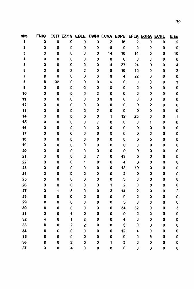
1

2

3

4

5

6

7

8

9

10

11

12

13

14

15

16

17

18

19

20

21

22

23

24

25

26

27

28

29

30

31

32

33

34

35

36

37

79

site ENIG ESTI EZON EBLE EWHI ECRA ESPE EFLA EGRA ECHL Esp 0 0 0 0 0 2 16 2 0 0 2

0 0 0 0 0 0 0 0 0 0 0 0 0 0 0 0 14 16 14 0 0 10

0 0 0 0 0 0 0 0 0 0 0

0 0 0 0 0 14 27 24 0 0 4

0 0 2 2 0 0 16 10 0 0 2

0 0 0 0 0 0 4 22 0 0 0

0 32 0 0 0 6 0 0 0 0 1

0 0 0 0 0 0 0 0 0 0 0

0 0 0 0 2 0 0 0 0 0 0

0 0 0 0 0 0 0 0 0 0 0

0 0 0 0 0 0 0 0 2 0 0

0 0 0 0 2 0 0 0 0 0 0

0 0 0 0 0 1 12 25 0 0 1

0 0 0 0 7 0 0 0 1 0 0

0 0 0 0 0 0 0 0 0 0 0

0 0 0 0 0 0 0 0 0 0 0

0 0 0 0 0 0 0 0 5 0 0

0 0 0 0 0 0 0 0 0 0 0

0 0 0 0 0 0 0 0 0 0 0

0 0 0 0 7 0 43 0 0 0 0

0 0 0 1 0 0 4 0 0 0 0

0 0 0 0 0 0 13 19 0 0 0

0 0 0 0 0 0 2 0 0 0 0

0 0 0 0 0 0 3 0 0 0 0

0 0 0 0 0 1 2 0 0 0 0

0 1 8 0 0 3 14 2 0 0 2

0 0 0 0 0 0 0 0 0 0 0

0 0 0 0 0 0 5 3 0 0 0

0 0 0 0 0 0 34 32 0 0 5

0 0 4 0 0 0 0 0 0 0 0

4 0 1 2 0 0 4 0 0 0 0

0 0 2 2 0 0 5 0 0 0 0

0 0 0 0 0 0 12 4 0 0 0

0 0 0 0 0 0 0 0 5 0 0

0 0 2 0 0 1 3 0 0 0 0

0 0 4 0 0 0 0 0 0 0 0

80

site ENIG ESTI EZON EBLE EWHI ECRA ESPE EFLA EGRA ECHL Esp 38 0 0 4 3 0 0 20 0 0 0 9 39 0 0 0 0 0 0 3 1 0 0 0

40 0 0 1 0 0 0 27 9 0 0 2 41 0 0 1 1 0 1 12 2 0 0 0 42 0 0 1 0 0 1 4 0 0 0 0 43 0 1 0 0 0 0 3 0 0 0 0 44 0 2 2 0 0 0 1 1 0 0 0 45 0 3 4 1 0 0 3 0 0 0 0 46 0 0 2 3 0 0 1 0 0 0 0 47 0 0 1 1 0 0 1 0 0 0 0

48 0 9 8 2 0 0 20 0 0 0 0 49 0 0 0 0 0 3 37 2 0 0 0 50 0 0 0 0 0 0 1 1 0 0 1 51 1 0 1 1 0 0 26 2 0 0 0 52 0 0 0 0 2 0 2 0 0 1 0 53 1 0 0 0 0 0 0 0 0 0 0

54 0 0 35 0 0 1 3 1 0 0 0 55 0 0 0 0 0 0 0 0 0 0 0 56 1 1 4 1 0 0 0 0 0 0 0 57 4 0 1 0 0 0 2 0 0 0 0

58 0 3 9 1 0 0 2 0 0 0 0

81

Appendix 3. Sites sampled in the Spring River basin during 1994 (sites 53-58) and 1995

(sites 1-52 ), with date of collection, geographic coordinates, and values of environmental

variables. Site numbers correspond to locations indicated in Figure 1. Abbreviations refer

to the following variables, with units of measurement in parentheses: date = day of the

month, lat = north latitudinal geographic coordinate (decimal degrees), long = west

longitudinal geographic coordinate (decimal degrees), riffle = riffle mesohabitat (%), run =

run mesohabitat (%), pool = pool mesohabitat (%), back = backwater mesohabitat (%),

mud = mud substratum (%), sand = sand substratum (%), gravel = gravel substratum (%),

smcob = small cobble substratum (%), 19cob = large cobble substratum (%), bould =

boulder substratum (%), bed = bedrock substratum (%), can = canopy cover (%), sub =

submergent vegetation (%), emerg = emergent vegetation (%), struct = woody structure

(%), DO = dissolved oxygen (mg/L), C02 = carbon dioxide (mg/L), alk = total alkalinity

(mg/L), hard = hardness (ppm), nitr = nitrate (mg/L), phos = phosphate (mg/L), temp =

water temperature (CO), pH = pH, DA = drainage area (km2), cs area = cross-sectional

area (m2), width = maximum stream width (m), alt = altitude (km), grad = gradient

(m/km). Missing values are denoted by 999.

123456

789

10111213141516171819202122232425262728293031323334353637

82

site date lat long riffle run pool back mud sand

17-18 May 36.76 94.02 60 38 2 0 0 1

18 May 37.41 94.72 0 45 0 55 60 34

23 May 36.77 94.02 20 40 20 20 0 5

23 May 36.73 93.97 1 0 99 0 70 5

24 May 36.79 94.03 40 35 5 20 5 2

25 May 37.07 94.11 10 60 0 30 15 2

25 May 37.04 94.06 15 65 5 15 2 1

26 May 37.03 93.99 60 15 10 15 20 5

30 May 37.03 94.78 20 5 65 10 21 40

30 May 37.06 94.80 7 13 60 20 60 30

31 May 37.08 94.74 0 90 0 10 75 22

1 June 37.05 94.82 0 2 98 0 94 5

5 June 37.44 94.72 10 88 0 2 61 2

6 June 36.86 94.35 80 10 0 10 1 1

1 August 37.18 94.82 20 70 0 10 34 20

13 June 37.55 94.71 5 70 20 5 80 2

13 June 37.56 94.72 5 0 95 0 70 20

14 June 37.21 94.83 5 0 93 2 84 5

14 June 37.13 94.80 0 0 95 5 69 5

15 June 37.53 94.72 10 20 68 2 85 5

16 June 37.31 94.65 30 30 20 20 20 10

19 June 37.53 94.25 5 80 0 15 10 5

20 June 37.41 94.10 37 43 10 10 18 2

20 June 37.36 94.04 40 5 50 5 1 4

21 June 37.12 93.90 50 40 3 7 2 1

21 June 36.96 93.86 12 6 80 2 3 10

22 June 36.90 94.13 20 70 2 5 2 5

27 June 37.34 94.63 2 3 85 10 93 3

28 June 36.99 94.68 50 40 0 10 3 6

29 June 36.97 94.56 50 45 0 5 1 3

7 July 37.28 94.53 87 10 0 3 1 2

8 July 37.27 94.52 55 35 0 10 2 10

9 July 37.06 93.84 999 999 999 999 2 1

10 July 37.34 94.02 60 20 15 5 1 0

10 July 37.40 94.30 0 100 0 0 48 48

11 July 37.28 94.51 10 50 0 40 5 30

11 July 37.28 94.52 5 60 5 30 4 20

83

site date lat long riffle run pool back mud sand 38 12 July 37.19 94.31 15 70 0 15 1 2

39 13 July 37.07 93.84 50 40 0 10 1 3

40 13 JUly 37.05 93.80 35 40 0 20 1 5

41 17 July 37.11 94.22 999 999 999 999 3 1

42 18 July 37.16 94.62 1 79 0 20 3 10

43 18 July 37.17 94.60 40 45 0 15 5 5

44 19 July 37.18 94.65 68 25 0 7 1 5

45 20 JUly 37.18 94.46 45 45 0 10 7 5

46 25 July 37.22 94.59 10 85 0 5 3 5

47 26 July 37.02 94.48 5 55 0 40 20 5

48 27 JUly 36.90 94.36 55 30 0 15 10 5

49 27 July 36.89 94.09 5 55 0 40 10 5

50 3 August 36.98 94.70 65 20 7 8 15 5

51 7 August 37.35 94.32 0 100 0 0 44 5

52 8 August 37.28 94.67 10 70 0 20 32 5

53 21 July 36.93 94.74 50 8 32 10 2 10

54 27-28 July 37.19 94.63 39 40 6 15 3 5

55 29 July 37.02 94.72 2 83 2 13 1 1

56 2 August 37.06 94.71 30 20 20 30 2 10

57 4 August 37.13 94.63 45 5 50 0 5 10

58 5 August 37.05 94.64 60 20 20 0 1 4

123456789

10111213141516171819202122232425262728293031323334

353637

84

site gravel smcob Igcob bould bed can sub emerg struct DO CO2 20 29 49 1 a 85 a 1 1 8 15

3 1 1 1 a 60 a a 15 6 25 50 24 20 1 a 30 a 20 10 7 20 10 10 5 a a 1 a a 2 11 25 31 31 30 1 a 2 a 5 1 9 25 30 31 15 5 45 2 2 a 5 9 25 30 50 11 5 1 85 a a 5 9 25 23 40 10 2 a 60 a a 5 8 20 20 10 5 2 2 55 2 a 5 7 15

9 a a 1 a 95 30 a 5 5 25 2 a a 1 a 30 a a 10 7 10 1 a a a a 5 20 29 a 5 20 2 30 5 a a 85 a a 15 6 30 4 9 4 1 80 20 5 5 5 9 20

20 10 10 5 1 85 60 5 20 5 25 7 5 5 1 a 10 20 25 2 7 15 3 2 a a 5 95 a a 15 7 15

10 1 a a a 90 a a 15 3 20 1 a a 20 5 60 a a 20 5 20 2 2 1 5 a 5 a 10 15 3 20

25 15 15 10 5 3 7 a 3 7 15 65 15 4 1 a 20 a 10 15 10 15 45 10 5 2 18 80 a 15 5 8 15 15 20 9 1 50 5 a a 1 10 15 50 36 10 1 a 30 1 3 10 7 25 25 40 20 2 a 35 a 5 2 8 25 43 39 10 1 a 25 a 5 999 8 20 2 a a 2 a 50 999 999 50 3 15

40 35 10 1 a 35 a 1 10 7 20 35 39 20 2 a 90 a a 2 6 15 27 55 10 3 2 15 a 3 2 5 20 44 35 4 5 a 5 80 30 5 6 20 35 50 12 a a 55 a 5 3 6 20 5 10 11 3 70 70 a 1 1 7 15 2 1 1 a a 80 a a 55 5 20

40 21 3 1 a 20 a 5 10 6 20 62 12 2 a a 20 a 3 5 5 20

85

site gravel smcob Igcob bould bed can sub emerg struct DO CO2 38 30 50 10 7 a 45 1 3 3 7 20 39 23 70 2 1 a 75 3 a 5 8 20 40 50 39 4 1 a 7 a 7 3 9 20 41 36 45 10 5 a 15 a 15 3 8 20 42 36 15 5 1 30 1 a 5 2 999 15 43 56 25 3 1 5 3 a a 2 7 25 44­ 73 20 1 a a 5 a a 1 8 15 45 35 40 10 3 a 3 a 4 2 7 15 46 48 30 12 2 a 15 a 15 1 7 20 47 44 30 1 a a 5 a 5 20 8 15 48 70 10 5 a a 15 a 5 15 7 15 49 45 35 5 a a 10 2 3 25 8 15 50 57 20 3 a a 75 a a 15 6 10 51 20 15 15 1 a 20 a 3 5 5 15 52 5 3 12 3 40 20 a 7 30 5 15 53 37 50 1 a a 1 a a 7 7 15 54 30 40 20 1 a 20 a a 5 8 20 55 2 3 3 3 87 1 a a 2 7 20 56 14 14 10 20 30 5 a a 20 8 15 57 40 40 5 a a 5 a a 7 7 20 58 29 50 15 1 a 15 a a 1 12 10

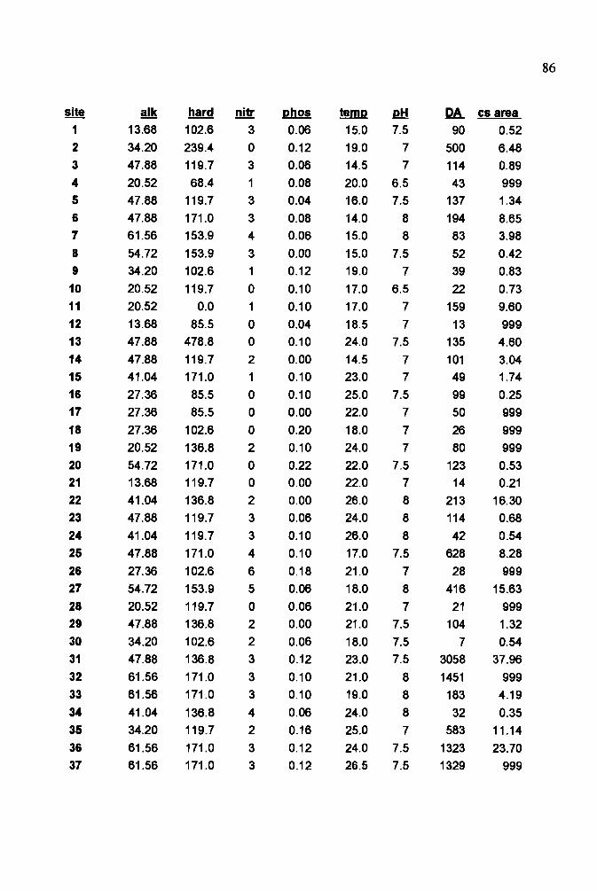
1

2

3

45

6

7

8

9

10

11

12

13

14

15

16

17

18

19

2021

22

23

24

25

26

27

28

29

30

31

32

33

34

35

36

37

86

site alk hard nitr phos temp .PH DA cs area 13.68 102.6 3 0.06 15.0 7.5 90 0.52

34.20 239.4 0 0.12 19.0 7 500 6.48 47.88 119.7 3 0.06 14.5 7 114 0.89 20.52 68.4 1 0.08 20.0 6.5 43 999 47.88 119.7 3 0.04 16.0 7.5 137 1.34 47.88 171.0 3 0.08 14.0 8 194 8.65 61.56 153.9 4 0.06 15.0 8 83 3.98

54.72 153.9 3 0.00 15.0 7.5 52 0.42

34.20 102.6 1 0.12 19.0 7 39 0.83

20.52 119.7 0 0.10 17.0 6.5 22 0.73 20.52 0.0 1 0.10 17.0 7 159 9.60

13.68 85.5 0 0.04 18.5 7 13 999 47.88 478.8 0 0.10 24.0 7.5 135 4.60

47.88 119.7 2 0.00 14.5 7 101 3.04 41.04 171.0 1 0.10 23.0 7 49 1.74

27.36 85.5 0 0.10 25.0 7.5 99 0.25

27.36 85.5 0 0.00 22.0 7 50 999

27.36 102.6 0 0.20 18.0 7 26 999

20.52 136.8 2 0.10 24.0 7 80 999

54.72 171.0 0 0.22 22.0 7.5 123 0.53 13.68 119.7 0 0.00 22.0 7 14 0.21

41.04 136.8 2 0.00 26.0 8 213 16.30 47.88 119.7 3 0.06 24.0 8 114 0.68

41.04 119.7 3 0.10 26.0 8 42 0.54

47.88 171.0 4 0.10 17.0 7.5 628 8.28

27.36 102.6 6 0.18 21.0 7 28 999 54.72 153.9 5 0.06 18.0 8 416 15.63

20.52 119.7 0 0.06 21.0 7 21 999

47.88 136.8 2 0.00 21.0 7.5 104 1.32

34.20 102.6 2 0.06 18.0 7.5 7 0.54 47.88 136.8 3 0.12 23.0 7.5 3058 37.96

61.56 171.0 3 0.10 21.0 8 1451 999

61.56 171.0 3 0.10 19.0 8 183 4.19

41.04 136.8 4 0.06 24.0 8 32 0.35

34.20 119.7 2 0.16 25.0 7 583 11.14

61.56 171.0 3 0.12 24.0 7.5 1323 23.70 61.56 171.0 3 0.12 26.5 7.5 1329 999

87

site alk hard nitr phos temp .PH DA cs area 38 68.40 171.0 4 0.06 22.0 7.5 1350 999 39 68.40 188.1 4 0.06 19.0 7.5 611 6.30 40 61.56 171.0 4 0.06 21.0 8 183 5.45 41 61.56 171.0 5 0.06 22.0 8 286 7.32 42 54.72 205.2 5 0.06 26.0 8 4757 999 43 61.56 188.1 5 0.14 25.5 8 771 9.01 44 61.56 171.0 4 0.06 25.0 8 3970 19.01 45 54.72 188.1 5 0.06 23.0 8 687 5.91 46 61.56 205.2 3 0.10 24.0 8 3191 20.66 47 61.56 153.9 4 0.06 23.0 8 1365 23.76 48 61.56 171.0 4 0.08 21.0 8 919 999 49 61.56 171.0 5 0.10 23.0 8 390 7.05 50 54.72 153.9 2 0.06 23.5 7.5 109 3.43 51 27.36 85.5 3 0.12 26.0 7 1157 17.25 52 41.04 376.2 4 0.14 27.0 7.5 707 3.43 53 47.88 205.2 2.5 0.12 26.0 8 7081 999 54 61.56 205.2 3 0.08 24.0 8 3202 999 55 47.88 171.0 3 0.08 25.0 8 6892 999 56 54.72 188.1 2.5 0.08 28.0 8.5 7885 999 57 75.24 273.6 4 0.46 24.0 8 4910 999 58 54.72 153.9 2.5 0.06 23.5 8 1464 999

1

23

45

67

89

10

11

1213

141516

171819

2021

2223

24

25

26

272829

30

31

32

33

34

353637

site width alt

7.2 418

14.6 268 13.8 418

4.0 451

19.5 412

22.9 326 29.4 341

15.8 378 15.2 245 6.6 253

16.2 241 3.3 270

10.4 274 9.3 322 7.7 259 6.0 293 2.0 293

6.0 268 33.5 253

4.2 287 1.8 262

51.0 280 19.6 302

1.8 322

16.5 328 7.6 421

19.2 331 12.0 268

8.0 236 8.5 312

50.0 256

999 259

10.0 341

7.0 323

13.0 271 40.0 256 30.5 256

88

grad

6.06

1.52

3.03

9.09

6.06

1.52 1.52

3.03 1.52

1.52

0.00 3.03 1.52

1.52 1.52 3.03 3.03

1.52 1.52

1.52 1.52

0.00 1.52

4.55 1.52

4.55 1.52 1.52

3.03

9.09 0.00

1.52

3.03

4.55

0.00 0.00 0.00

89

site width alt grad 38 21.5 280 0.00 39 9.5 332 1.52 40 18.0 352 1.52 41 15.8 299 1.52

42 46.3 247 0.00 43 17.0 247 0.00

44 54.9 247 0.00

45 22.0 265 0.00 46 50.5 250 0.00

47 46.0 274 0.00

48 50.0 296 0.00 49 18.0 338 3.03 50 15.0 232 1.52 51 23.7 268 0.00

52 11.0 256 0.00 53 75.0 223 0.00

54 35.0 247 0.00

55 63.0 235 0.00

56 345.0 238 0.00 57 32.0 244 0.00 58 22.0 247 0.00

I

I, Christopher David Wilkinson, hereby submit this thesis to Emporia State University as partial fulfillment of the requirements for an advanced degree. I agree that the Library of the University may make it available to use in accordance with its regulations governing materials of this type. I further agree that quoting, photocopying, or other reproduction of this document is allowed for private study, scholarship (including teaching) and research purposes of a nonprofit nature. No copying which involves potential financial gain will be allowed without written permission of the author.

~/e. I'f11­Date

Spatial Pattern ofFish Assemblage Structure and Environmental Correlates in the Spring

Riyer Basin, with Emphasis on the Neosho Madtom (Noturus placidus) Title of Thesis

I I

2A"2~/~U /7/ /99/ Date Received

,j ;(1'

/1/

) v~ g'.. .1.1.. .... ~