
American Journal of Environmental Science and Engineering...
16
American Journal of Environmental Science and Engineering 2018; 2(1): 1-16 http://www.sciencepublishinggroup.com/j/ajese doi: 10.11648/j.ajese.20180201.11 Report Analysis of Mt Kenya Glaciers Recession Using GIS and Remote Sensing Purity Njeri Mwaniki * , David Kuria, Charles Ndegwa Mundia, Godfrey Makokha Institute of Geomatics, GIS and Remote Sensing in Dedan Kimathi University of Technology, Nairobi, Kenya Email address: * Corresponding author To cite this article: Purity Njeri Mwaniki, David Kuria, Charles Ndegwa Mundia, Godfrey Makokha. Analysis of Mt Kenya Glaciers Recession Using GIS and Remote Sensing. American Journal of Environmental Science and Engineering. Vol. 2, No. 1, 2018, pp. 1-16. doi: 10.11648/j.ajese.20180201.11 Received: March 26, 2018; Accepted: April 16, 2018; Published: May 17, 2018 Abstract: This research analyses the changes in coverage Mt Kenya glaciers in a bid find what has been causing the retreat of these glaciers. Optical Landsat data for 1984 to 2017 and Climatic data of the same years were used. Glaciers and forest coverage were extracted from Landsat images and its thermal band was used to extract temperature data. Correlation with the respective year’s climatic data and forest cover area were done to justify the assumption that the shrinkage in the glaciers coverage has been caused by changes in climate and/or deforestation. Then using the historical EC Earth model climate data predictions for 1984-2017 and historical observed data for the same years, bias correction factors were computed and used to correct the future model data for the years (2018-2045). Since the data was extracted for only four points around Mt Kenya, Interpolation was then done to obtain the Precipitation and Temperature for the mountain peak (since the glaciers are found at the peak) using the IDW technique. Prediction of glacier area coverage was then done using these interpolated climate data. In order to predict the future glacier cover, linear equations of the form y = a 1 x 1 + a 2 x 2 +b o of the interpolated climate data (for 2018-2045) and computed glacier areas for (1984-2017) were formed. The a 1 a 2 and b o in the equation are constants obtained from SPSS (a statistical software). X1 and x2 are the predicted Temperature and Precipitation respectively. Predictions were done for RCP scenarios 8.5 and 4.5. The results of prediction showed that the current trend of glacier thinning is going to continue but at a slower rate compared to the rapid melting that was observed for the period 1984-2017. However, Mt Kenya glaciers are likely to have completely disappeared by the year 2100. Keywords: Glaciers and Forest Coverage, Climate, Prediction 1. Introduction The term glacier refers to a perennial natural body of surface ice which visibly moves under its own weight in response to gravitational force. Glaciers move from upper reaches with a net gain of ice mass to lower regions where mass loss dominates [1]. Although glaciers are generally thought of as polar entities, they also are found in mountainous areas throughout the world, on all continents except Australia and even at or near the Equator on high mountains in Africa and South America [2]. In East Africa, glaciers began to recede in the 1880's [3]. Well-documented examples of glacial recession in East Africa include the Mount Kenya, Ruwenzori and Kilimanjaro glaciers. The widespread retreat is all the more notable because these tropical mountain glaciers are old. They have survived thousands of years of natural climate fluctuations, only to dwindle at a time when other climate indicators are showing the results of human influence on climate. The problem thus, is to determine which of the many characteristics of climate change they are indicating and to what extent these changes can be attributed to the train of events set in motion by increased of human production of greenhouse gases [4]. Variations in many conditions can influence glacial melt this includes precipitation, humidity, temperature, cloud cover, increased solar radiation and direct evaporation from the glacier surface and the mountain’s relief [5].
Transcript of American Journal of Environmental Science and Engineering...

American Journal of Environmental Science and Engineering 2018; 2(1): 1-16
http://www.sciencepublishinggroup.com/j/ajese
doi: 10.11648/j.ajese.20180201.11
Report
Analysis of Mt Kenya Glaciers Recession Using GIS and Remote Sensing
Purity Njeri Mwaniki*, David Kuria, Charles Ndegwa Mundia, Godfrey Makokha
Institute of Geomatics, GIS and Remote Sensing in Dedan Kimathi University of Technology, Nairobi, Kenya
Email address:
*Corresponding author
To cite this article: Purity Njeri Mwaniki, David Kuria, Charles Ndegwa Mundia, Godfrey Makokha. Analysis of Mt Kenya Glaciers Recession Using GIS and
Remote Sensing. American Journal of Environmental Science and Engineering. Vol. 2, No. 1, 2018, pp. 1-16.
doi: 10.11648/j.ajese.20180201.11
Received: March 26, 2018; Accepted: April 16, 2018; Published: May 17, 2018
Abstract: This research analyses the changes in coverage Mt Kenya glaciers in a bid find what has been causing the retreat of
these glaciers. Optical Landsat data for 1984 to 2017 and Climatic data of the same years were used. Glaciers and forest coverage
were extracted from Landsat images and its thermal band was used to extract temperature data. Correlation with the respective
year’s climatic data and forest cover area were done to justify the assumption that the shrinkage in the glaciers coverage has been
caused by changes in climate and/or deforestation. Then using the historical EC Earth model climate data predictions for
1984-2017 and historical observed data for the same years, bias correction factors were computed and used to correct the future
model data for the years (2018-2045). Since the data was extracted for only four points around Mt Kenya, Interpolation was then
done to obtain the Precipitation and Temperature for the mountain peak (since the glaciers are found at the peak) using the IDW
technique. Prediction of glacier area coverage was then done using these interpolated climate data. In order to predict the future
glacier cover, linear equations of the form y = a1x1 + a2x2 +bo of the interpolated climate data (for 2018-2045) and computed
glacier areas for (1984-2017) were formed. The a1 a2 and bo in the equation are constants obtained from SPSS (a statistical
software). X1 and x2 are the predicted Temperature and Precipitation respectively. Predictions were done for RCP scenarios 8.5
and 4.5. The results of prediction showed that the current trend of glacier thinning is going to continue but at a slower rate
compared to the rapid melting that was observed for the period 1984-2017. However, Mt Kenya glaciers are likely to have
completely disappeared by the year 2100.
Keywords: Glaciers and Forest Coverage, Climate, Prediction
1. Introduction
The term glacier refers to a perennial natural body of
surface ice which visibly moves under its own weight in
response to gravitational force. Glaciers move from upper
reaches with a net gain of ice mass to lower regions where
mass loss dominates [1]. Although glaciers are generally
thought of as polar entities, they also are found in
mountainous areas throughout the world, on all continents
except Australia and even at or near the Equator on high
mountains in Africa and South America [2].
In East Africa, glaciers began to recede in the 1880's [3].
Well-documented examples of glacial recession in East Africa
include the Mount Kenya, Ruwenzori and Kilimanjaro
glaciers. The widespread retreat is all the more notable
because these tropical mountain glaciers are old. They have
survived thousands of years of natural climate fluctuations,
only to dwindle at a time when other climate indicators are
showing the results of human influence on climate. The
problem thus, is to determine which of the many
characteristics of climate change they are indicating and to
what extent these changes can be attributed to the train of
events set in motion by increased of human production of
greenhouse gases [4].
Variations in many conditions can influence glacial melt
this includes precipitation, humidity, temperature, cloud cover,
increased solar radiation and direct evaporation from the
glacier surface and the mountain’s relief [5].

2 Purity Njeri Mwaniki et al.: Analysis of Mt Kenya Glaciers Recession Using GIS and Remote Sensing
In East Africa, the dramatic shrinking of Kilimanjaro’s
glaciers has attracted global attention [6]. The ice on Mount
Kilimanjaro has been retreating both in thickness and in area,
with the latter’s decline being the most dramatic [7].
Compared to 1800 when the ice covered about 20 km2, by
2003, the area had shrunk to about 2.51 km2 [8]. An estimated
82 per cent of the ice cap that crowned the mountain when it
was first thoroughly surveyed in 1912 is now gone, and the
remaining ice is thinning by as much as a meter per year in one
area. According to some projections, if recession continues at
the present rate, the majority of the remaining glaciers on
Kilimanjaro could vanish by 2020 [9]. Other studies have
showed that deforestation around Mt Kilimanjaro has affected
the climate around it and as result, it is being considered as one
of the contributing factors to the thinning of glaciers being
experienced there [10-11].
On the other hand, Mt. Ruwenzori glaciers occur on only three
of the range’s peaks: Stanley, Speke and Baker. The glacial
recession on the Ruwenzori Mountain has been attributed to
higher air temperatures and less snow accumulation during the
20th century [12]. It is also possible that decreasing cloud
cover over the same time has contributed to vaporization of
these glaciers [12]. On one visit in 1974, it was estimated that
since 1958, the Speke Glacier had retreated by 30 to 40 m and
shrunk laterally by 10 to 20 m [5].
In Kenya, studies of the Lewis Glacier (which is the largest
glacier) on Mount Kenya found that higher temperatures
during the 1900s were a greater cause of its shrinking than sun
exposure [7]. Other studies have shown that some warming
during the 20th century and associated rises in atmospheric
humidity, along with a possible contribution of continued
solar radiation forcing are the causes of Mount Kenya’s recent
ice losses [13].
Mount Kenya lost 92 % of its ice cap in the last century. Of
the 18 ice entities that covered the mountain peaks, at the end
of the 19th century, 9 had disappeared altogether and all
suffered substantial loss [14]. The Gregory glacier, which
joined with the Lewis on one end, was the latest victim having
disappeared by March 2011 and only debris covered ice
remnants of unknown thickness are left [15].
In Kenya, the forest cover dramatically decreased such that
in 1986 a presidential declaration led to banning of
exploitation of indigenous forest. From time-to-time,
licensees would put up a case claiming to be allowed to
remove materials pre-felled and paid for, that they had not
been able to collect by the time the ban was announced.
Individual cases were authorized on occasion but
complications emerged as authorization was abused and fresh
logging took off again. Even though the ban was issued back
in 1986, individuals have continued to apply for permits that
have been approved as recently as this year. Large scale
logging of indigenous forests exists today more than ever
before despite the ban [16].
The magnitude of forest destruction is very high. This may
have significantly affected the climate of the areas around the
mountain and consequently it may have led to glacier
recession.
2. Data and Methodology
2.1. Study Area
The Mount Kenya is the second highest mountain in Africa
after Mt Kilimanjaro, it is an isolated, extinct, denuded
volcano (before glaciation it was 7000m high) was built up by
intermittent volcanic eruptions between 3.1 and 2.6 million
years ago [17]. It was covered by an icecap for thousands of
years and this resulted in very eroded slopes [18]. The highest
peaks of the mountain are Batian (5199m), Nelion (5188m)
and point Lenana (4985m).
It lies on the equator (0°6’S, 37°18’E), approx. 150 km
NNE of Nairobi. The mountain is located in the Mount Kenya
National Park, which is a designated protected area. The
national park covers an area of 700 square kilometres and was
established in 1949 [19].
The climate of Mt. Kenya region is largely determined by
altitude. Average temperatures decreases by 0.60C for each
100m increase in altitude. An afro-alpine type of climate,
typical of the tropical East African high mountains,
characterizes the higher ranges of Mt. Kenya. The altitudes
with the highest rainfall are between 2,700 and 3,100m, while
above 4,500m most precipitation falls as snow or hail. Frosts
are common above 2500 above mean sea level [20].
Rainfall pattern in Mt Kenya ecosystem is bimodal. It
ranges from 900 mm in the north Leeward side to 2,300 mm
on the southeastern slopes (Windward side) of the mountain
(Survey of Kenya, 1966) with maximum rains falling during
months of March to June and October to November. The driest
months are January and February with the windward side
experiencing the strongest effects of the trade wind system
[20].
The mountain is one of the five main water towers of Kenya,
the others being the Aberdare ranges, Mau complex, Mt.
Kenya and Cherangani hills. Mt. Kenya is the source of two of
Kenya’s largest rivers, the Tana and Ewaso Nyiro [20].
Vegetation types and species distribution are distinguished
according to the different climatic zones and altitudes, most
obviously through variation in vegetation structure, cover and
composition.
The following vegetation zones are apparent from the high
altitudes to lower altitudes.
(i) Moorland
This lies between 3000m and 3500m. It’s also referred to as
Ericaceous belt and is mainly covered with giant heath,
African sage (Artemisia afra) and several Gentians (Swertia
spp). It is also characterized by smaller trees in glades, such as
the East African Rosewood (Hagenia abyssinica) and St.
John’s Wort (Hypericum spp). Trees are covered with moss
and lichens (Usnea spp).
(ii) Pure Bamboo
This is a pure bamboo (Arudinaria spp) zone occurring
between 2550 and 2650 above mean sea level. The main
purpose was supplying commercial forest products to the
forest industries located within the forest adjacent areas. Main
commercial tree species planted include Cypress, Pines, and
Eucalypts.

American Journal of Environmental Science and Engineering 2018; 2(1): 1-16 3
(iii) Nyayo Tea Zone
This area was opened up by the Nyayo Tea Zones
Development Corporation in 1986 with the aim of promoting
forest conservation by providing a buffer zone to check
against human encroachment into forest reserves [20].
Mt. Kenya Forest Reserve is also home to a wide diversity
of fauna. These include African elephant, leopard, giant forest
hog, Bongo and the black fronted duiker. There are also over
ten species of ungulates in Mt. Kenya forest reserve. These
include the duiker, bushbuck, deffassa waterbuck, mountain
reedbuck, bush pig, the common zebra, eland, steenbok,
Harveys red duiker and common duiker. These animals are
spread over the entire ecosystem but their densities are low in
the southern slopes. Cape buffaloes occur on the western
slopes of the mountain but are rare on the eastern slopes
possibly because of their preference for open bushland.
Several primates are found in Mt. Kenya forest reserve, the
most common being the black and white colobus and Sykes
monkey. These primates are widely spread within the forest
reserve [20] .
Communities living adjacent to Mount Kenya Forest are
mainly agriculturists. The Kikuyu community occupy the
western side of Mount Kenya, Meru people on the eastern side,
while to the south is the Embu ethnic group. Other tribes that
interact with the ecosystem include the pastoralist
communities who occupy the northern part of the mountain.
The total population of the community that live within the
districts that border the ecosystem was 17.6 million in 1999
(1999 Kenya population census data).
Land ownership within the area falls under different
categories of land tenure. The agricultural lands - both
large-scale (horticulture and floriculture) and small scale are
held under freehold (Private ownership), whereas ranches and
sanctuaries are held under leasehold as government lands.
Other types of land tenures include public lands and trust land
[20].
Agriculture is the main economic activity in the areas
adjacent to the forest reserve. The type of agriculture practiced
and productivity potential depend mainly on altitude, which in
turn determines the temperatures and amount of rainfall. On
the eastern and southern side of the mountain, where rainfall is
high, intensive arable farming is practiced. In the upper areas,
potatoes, pyrethrum and tea are grown. In the mid-latitudes
zones, coffee, maize, beans, rice and bananas and mixed
livestock farming are practiced, while in the lower zones,
tobacco, cotton, sorghum, millet, pigeon peas and cow peas
are most dominant crops [20].
Mt Kenya ecosystem has attractive sceneries and great
potential for tourism development, which is yet to be fully
harnessed. The ecosystem is endowed with unique
geomorphologic features, cultural and historical sites that are
of great tourism attraction. In addition, there is a diversity of
wildlife populations which attract visitors. The ecosystem
supports tourism in the region by offering a diversity of
activities such as bird watching, trout fishing, walking and
wilderness trails [20]. Figure 1 shows the area of study.
Figure 1. Study Area.
2.2. Data
Most of the Landsat images used for this study (as shown in
table 1), can be downloaded from Earth Explorer and
GLOVIS websites. Historical climate data was also available
online in the NASA POWER website in terms of daily
observations from the year 1983. NASA POWER is a
renewable energy resource website of global meteorological
4 Purity Njeri Mwaniki et al.: Analysis of Mt Kenya Glaciers Recession Using GIS and Remote Sensing
and surface solar energy climatology data form NASA
satellites, at a resolution of 1⁰ by 1⁰. Precipitation data was
downloaded as raster from the Climate Hazards Infrared
Precipitation with Station data (CHIRPS) website, then
extracted to values using the coordinates of the point of
interest. CHIRPS is a Quasi – global rainfall dataset spanning
50⁰ S – 50⁰ N and dating back to 1981. It incorporates 0.05⁰ resolution satellite imagery with in-situ station data to create
gridded rainfall time series for trend analysis and seasonal
drought monitoring. The modelled climatic data (temperature
and rainfall) were extracted from the EC Earth model for
Representative Concentration Pathways (RCPs) 4.5 and 8.5.
Table 1. Types of Data and Sources.
Type of image sensor date of acquisition Path/row spatial resolution source
Landsat 5 TM 17/12/1984 160/60 30M RCMRD
Landsat 5 TM 25/05/1987 168/60 30M RCMRD
Landsat 5 TM 12/03/1992 168/60 30M Earth Explorer
Landsat 5 TM 22/05/1995 168/60 30M RCMRD
Landsat 7 ETM 21/02/2000 168/60 30M RCMRD
Landsat 7 ETM+ 06/05/2005 168/60 30M GLOVIS
Landsat 5 TM 20/11/2009 168/60 30M GLOVIS
Landsat 7 ETM+ 25/03/2012 168/60 30M GLOVIS
Landsat 7 ETM+ 02/03/2015 168/60 30m Earth Explorer
Landsat 7 ETM+ 26/05/2017 168/60 30m Earth Explorer
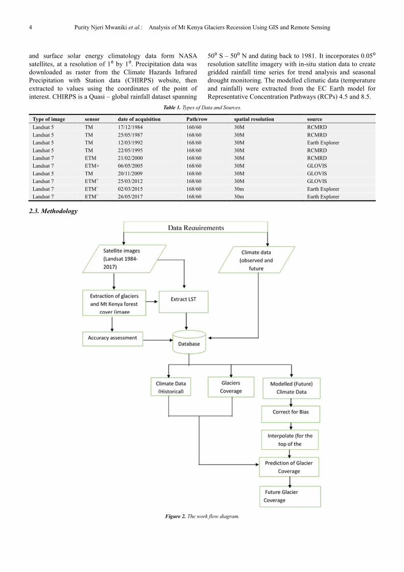
2.3. Methodology
Figure 2. The work flow diagram.

American Journal of Environmental Science and Engineering 2018; 2(1): 1-16 5
The Landsat7 image for the years 2005, 2012,2015 and
2017 had missing scan lines and had to be destripped using the
Landsat gap fill plugin and the gap mask which was provided
with the images.
The area of interest (AOI) was then subset but because of
cloud cover, it was not possible to use a shapefile of the whole
of Mt Kenya to subset all the images uniformly. On some of
the images, clouds occurred too close to the mountain peak,
which was the area with the most snow cover. Therefore, an
irregular AOI was generated manually and used to subset all
the other images.
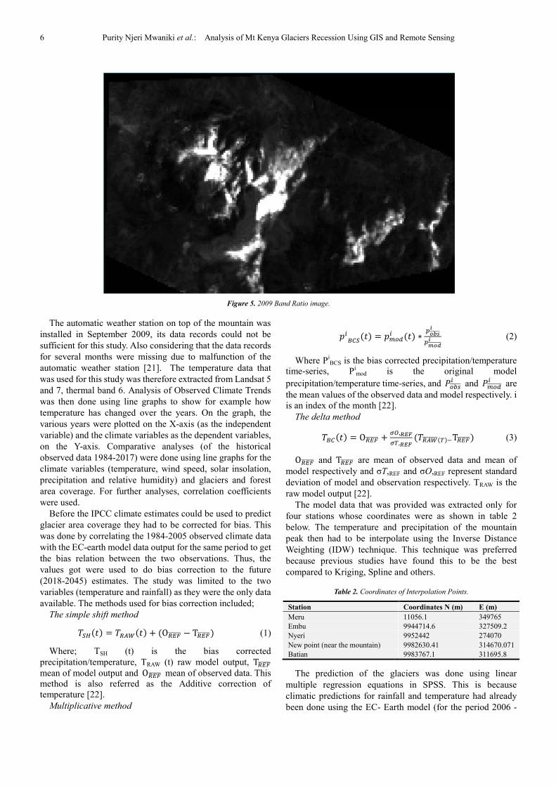
Computation of band ratio is the best method of
differentiating between glaciers and non-glacier areas in an
image [4].
������� �����4
����5
The raster images that resulted from band rationing were
single layer from which it was not possible to compute the
areas of the various layers of interest therefore, since one of
the objectives of this research was to compute area differences,
supervised classification was the best option. Band rationing
separates the melted glacier areas and the solid glacier areas
therefore; it was used as a guide when selecting the training
areas for the glaciers as can be shown by figures 7, 8 and 9 but
could not be used as the source of the training data since it is a
black and white.
Figure 3. 1984 Band Ratio image.
Figure 4. 1987 Band Ratio image.
6 Purity Njeri Mwaniki et al.: Analysis of Mt Kenya Glaciers Recession Using GIS and Remote Sensing
Figure 5. 2009 Band Ratio image.
The automatic weather station on top of the mountain was
installed in September 2009, its data records could not be
sufficient for this study. Also considering that the data records
for several months were missing due to malfunction of the
automatic weather station [21]. The temperature data that
was used for this study was therefore extracted from Landsat 5
and 7, thermal band 6. Analysis of Observed Climate Trends
was then done using line graphs to show for example how
temperature has changed over the years. On the graph, the
various years were plotted on the X-axis (as the independent
variable) and the climate variables as the dependent variables,
on the Y-axis. Comparative analyses (of the historical
observed data 1984-2017) were done using line graphs for the
climate variables (temperature, wind speed, solar insolation,
precipitation and relative humidity) and glaciers and forest
area coverage. For further analyses, correlation coefficients
were used.
Before the IPCC climate estimates could be used to predict
glacier area coverage they had to be corrected for bias. This
was done by correlating the 1984-2005 observed climate data
with the EC-earth model data output for the same period to get
the bias relation between the two observations. Thus, the
values got were used to do bias correction to the future
(2018-2045) estimates. The study was limited to the two
variables (temperature and rainfall) as they were the only data
available. The methods used for bias correction included;
The simple shift method
������ � ������� � �O��������� � T���������� (1)
Where; TSH (t) is the bias corrected
precipitation/temperature, TRAW (t) raw model output, T���������
mean of model output and O��������� mean of observed data. This
method is also referred as the Additive correction of
temperature [22].
Multiplicative method
��� ���� � �!"#� ��� ∗
%&'(������)
%*&+�������) (2)
Where PiBCS is the bias corrected precipitation/temperature
time-series, Pimod is the original model
precipitation/temperature time-series, and ,"-.������ and ,!"#�������
� are
the mean values of the observed data and model respectively. i
is an index of the month [22].
The delta method
�� ��� � O��������� �/0,234
/5,234�������������5�6T���������� (3)
O��������� and T��������� are mean of observed data and mean of
model respectively and σT,REF and σO,REF represent standard
deviation of model and observation respectively. TRAW is the
raw model output [22].
The model data that was provided was extracted only for
four stations whose coordinates were as shown in table 2
below. The temperature and precipitation of the mountain
peak then had to be interpolate using the Inverse Distance
Weighting (IDW) technique. This technique was preferred
because previous studies have found this to be the best
compared to Kriging, Spline and others.
Table 2. Coordinates of Interpolation Points.
Station Coordinates N (m) E (m)
Meru 11056.1 349765
Embu 9944714.6 327509.2
Nyeri 9952442 274070
New point (near the mountain) 9982630.41 314670.071
Batian 9983767.1 311695.8
The prediction of the glaciers was done using linear
multiple regression equations in SPSS. This is because
climatic predictions for rainfall and temperature had already
been done using the EC- Earth model (for the period 2006 -

American Journal of Environmental Science and Engineering 2018; 2(1): 1-16 7
2100) and the data for the two variables was acquired from
Kenya Meteorological Department (KMD). Using these
climate predictions, linear equations of the form
y = a1x1 + a2x2 +bo were formed,
Where y = glacier coverage being predicted
a1 a2 and bo are constants obtained from SPSS.
X1 and x2 are the predicted Temperature and rainfall.
Figure 2 summarises the procedure that is explained here.
3. Results and Discussion
From the results of image classification, glacier recession
has not been on a constant decline but there had been some
years where there was a constant accumulation of ice. This
trend can be shown by line graph (figure 6) and the classified
images (figure 7 – 12).
Figure 6. Mt Kenya Glacier Coverage Trend Curve.
3.1. The Classified Images
Some of the classified images that were used compute the areas of the glaciers for this study are shown by figures 7 -12.
Figure 7. 1984 Glacier Coverage Classified Image.
8 Purity Njeri Mwaniki et al.: Analysis of Mt Kenya Glaciers Recession Using GIS and Remote Sensing
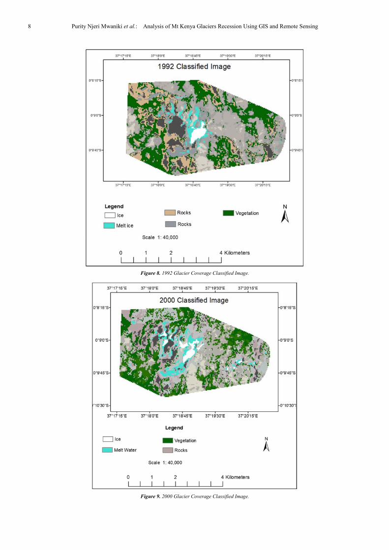
Figure 8. 1992 Glacier Coverage Classified Image.
Figure 9. 2000 Glacier Coverage Classified Image.

American Journal of Environmental Science and Engineering 2018; 2(1): 1-16 9
Figure 10. 2009 Glacier Coverage Classified Image.
Figure 11. 2012 Glacier Coverage Classified Image.

10 Purity Njeri Mwaniki et al.: Analysis of Mt Kenya Glaciers Recession Using GIS and Remote Sensing
Figure 12. 2017 Glacier Coverage Classified Image.
The area coverage of Mt Kenya forest declined from 1984 to 1987 but between 1995 and 2012 the pace of decline reduced, this
coverage is again on the decline as can be show by the trend curve below (figure 13).
Figure 13. The Trend of Mt forest cover.
3.2. The Relationship between Changes in Forest Cover and
Climate Variables
In order to determine the degree of relationships between
the various variables and glacier recession, correlation
coefficients (R) and coefficients of determination (R2) were
computed.
The changes in forest cover seemed to have had an effect on
the climate variables. Increased forest cover had a negative
correlation with temperature and humidity (it caused them to
decrease). The same forest cover had a negative relationship
with precipitation in that rainfall decreased despite increased
forest cover. The wind speeds however increased with the
increase in forest cover whereas solar insolation decreased
with increase in forest cover. These correlations are shown on
table 3.

American Journal of Environmental Science and Engineering 2018; 2(1): 1-16 11
Table 3. Climate variables Vs Forest Cover Correlation.
Forest cover vs Climate Variables Correlation Coefficient (R) Coefficient of Determination (R2) Magnitude of Correlation
Forest cover vs temperature -0.523 0.2737 = 28% moderate
Forest cover vs relative humidity -0.45433 0.2064 = 21% moderate
Forest cover vs precipitation -0.33414 0.1116 = 11% weak
Forest cover vs wind speed 0.5931 0.3518 = 35% moderate
Forest cover vs solar insolation -0.23994 0.0576 = 6% weak
3.3. The Relationship Between Forest Cover, Climate
Variables and Glacier Coverage
The relationship between relative humidity and glacier
cover was negative and weak with R= -0.225. The more the
relative humidity was, the less glacier accumulation. Relative
humidity was found responsible for R2 = 0.051 = 5% of the
changes in glacier coverage that occurred (figure 14).
Figure 14. Glacier Coverage Vs Relative Humidity.
Figure 15. Glacier Coverage Vs Temperature.
Figure 16. Glacier Coverage Vs Precipitation.
Figure 17. Glacier Coverage Vs Wind Speed.
Figure 18. Glacier Coverage Vs Solar Insolation.
Figure 19. Glacier Coverage Vs Forest Cover.
The temperature and glaciers coverage had a negative and
moderate correlation R= - 0.40583. It showed that the lower
the temperature the more the glacier accumulation and vice
versa. Temperature was responsible for R2= 0.1647 = 16% of
the changes in glacier coverage (figure 15).
The precipitation and glacier coverage had a moderate and
negative correlation of R = -0.45764. This showed that the

12 Purity Njeri Mwaniki et al.: Analysis of Mt Kenya Glaciers Recession Using GIS and Remote Sensing
more the rainfall, the less the glacier coverage. Rainfall was
found to have been responsible of R2 = 0.2094 = 21% of the
changes in glacier coverage recorded (figure 16).
Wind speed had a positive and moderate correlation with
the glacier coverage. R = 0.617739. The more the wind speed
the more the glacier accumulation was. This can be explained
as; the accelerated wind speed lead to more cooling of air at
the top of the mountain which resulted in more precipitation
thus accelerate glacier accumulation. Wind speed caused 38%
of glacier loss experienced during the period of study (figure
17).
For solar insolation, the assumption was that the more the sun
exposure, the more the rate of glacier melt but there was barely
any correlation with R= -0.09932. This meant that the more
the sun exposure the less the ice accumulation. Sun exposure
was responsible of 1% of the glacier loss. R2
= 0.009 =1 %
(figure 18).
The relationship between forest and glaciers cover was
positive and very strong (R = 0.864576). Forest cover was
responsible was responsible for 75% of the changes in glacier
coverage that occurred during the period of study. R2 = 0.7475
= 75%. This meant the more the forest cover, the more the
glacier coverage (figure 19).
3.4. Glacier Prediction
To predict glacier coverage, temperature and rainfall were
used as they were the only variables available. Bias correction
had to be done because like in any other estimate, climate
predictions are prone to bias.
In figures 20 and 21 the observed temperature and rainfall
data for 1978-2005 are compared against model estimates for
the same period for the one of the interpolating stations.
Figure 20. Comparison of Historical Observed rainfall and uncorrected estimates.
Figure 21. Comparison of Historical Observed Temperature and uncorrected estimates.
Where Janmodel is the model estimate and Janobs is the
observed data for the same period. Obs data stands for
observed rainfall for the same period. From figure 20, rainfall
model data appears to be overestimated compared to
temperature.
The climate estimates were extracted from the EC-Earth
model for both temperature and rainfall, for RCP4.5 and
RCP8.5. Computation of correction factors (i.e. the mean and
standard deviation) of historical data were then done using the
Simple Shift, Multiplicative and Delta methods explained in
section 2.2.
American Journal of Environmental Science and Engineering 2018; 2(1): 1-16 13
a
b
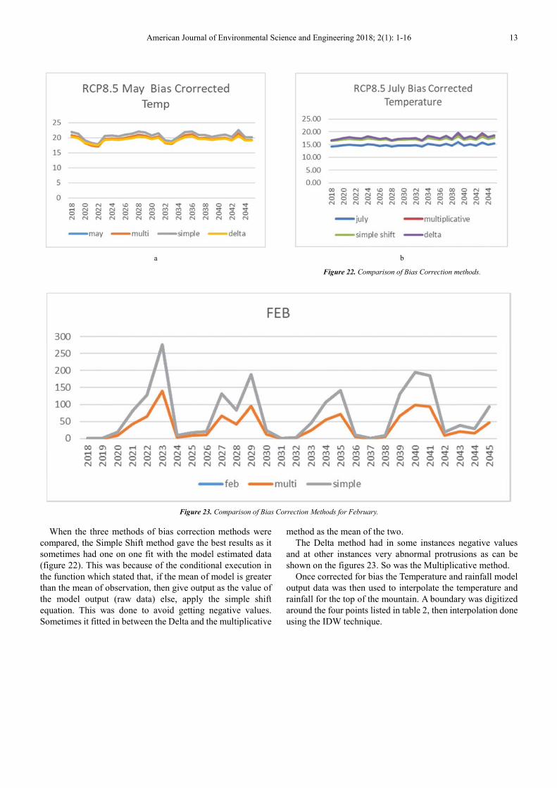
Figure 22. Comparison of Bias Correction methods.
Figure 23. Comparison of Bias Correction Methods for February.
When the three methods of bias correction methods were
compared, the Simple Shift method gave the best results as it
sometimes had one on one fit with the model estimated data
(figure 22). This was because of the conditional execution in
the function which stated that, if the mean of model is greater
than the mean of observation, then give output as the value of
the model output (raw data) else, apply the simple shift
equation. This was done to avoid getting negative values.
Sometimes it fitted in between the Delta and the multiplicative
method as the mean of the two.
The Delta method had in some instances negative values
and at other instances very abnormal protrusions as can be
shown on the figures 23. So was the Multiplicative method.
Once corrected for bias the Temperature and rainfall model
output data was then used to interpolate the temperature and
rainfall for the top of the mountain. A boundary was digitized
around the four points listed in table 2, then interpolation done
using the IDW technique.

14 Purity Njeri Mwaniki et al.: Analysis of Mt Kenya Glaciers Recession Using GIS and Remote Sensing
Figure 24. Results of Temperature Interpolation in ARCGIS using IDW Technique.
From the resultant raster like the one shown in figure 24,
extraction of temperature and rainfall for a point on top of the
mountain whose coordinates were (9983767.1 MN,
311695.8ME) was done. The interpolation results for both
variables based on RCP8.5 and RCP 4.5 bias corrected
temperature and rainfall for the top of the mountain are shown
in the figure 25 and 26 below.
Figure 25. Predicted Temperature trend based on both RCP 8.5 and RCP 4.5.
Figure 26. Predicted rainfall trend based on both RCP 8.5 and RCP 4.5.
RCP8.5 is a scenario that is characterized by increase in
greenhouse emission over the years. From figure 25 it can be
seen that compared to RCP 4.5 the temperature based on
RCP8.5 will be higher over the span of the period of study.
RCP4.5 is a stabilization scenario in which total radiative
forcing is stabilized shortly after 2100, without overshoot by
the application of a range of technologies and strategies for
reducing greenhouse gas emissions. Therefore, RCP 4.5 is a
more reliable scenario compared to 8.5.
Given that RCP4.5 is a stabilization scenario, if the climate
stabilises where it is now, the amount of precipitation being
received on Mt Kenya will decrease and reach its lowest in
2021 after which it will gradually increase and dip again in
2030. Based on RCP8.5 the same will have several peaks and
lows as can be shown by figure 26.
3.5. Predicted Glacier Coverage
The predicted temperature and precipitation above were
then input in SPSS (a statistical analysis Software) in order to
form an equation of the form y = a1x1 + a2x2 +bo. For the
RCP8.5, x1, x2 and bo were -0.455, 0.381 and -157.083. For
RCP 4.5 x1, x2 and bo were -0.175, 0.579 and -227.409. a1 and
a2 were the predicted temperature and precipitation
respectively.
The predicted glacier coverage is as shown in the figure 27.
From the figure it can be seen that just like 1984 to 2017 where
the glacier coverage did not have a steady decline but it
appeared to peak and decline alternately, so did the predicted
glacier coverage. This suggested that although the glacier
coverage is going to thin down, it would not do so in a straight
line of decline.

American Journal of Environmental Science and Engineering 2018; 2(1): 1-16 15
Figure 27. Predicted Glacier Coverage based on RCP4.5 and RCP8.5.
4. Conclusion and Recommendation
4.1. Conclusion
As can be shown on figure 6, the glacier cover on Mt Kenya
has not been steadily decreasing but there has been years
where there has been an increase.
From the results of correlation obtained, it came out forest
had the largest correlation with glacier coverage. Suggesting
that if forest can be increased, glacier coverage would increase.
The correlation between glacier coverage and forest cover was
very strong (R = 0.864576) therefore forest cover was
responsible was responsible for 75% of the changes in glacier
coverage that occurred during the period of study.
Temperature had a negative and moderate correlation R= -
0.40583. This meant that lower temperature would lead to
more glacier accumulation and vice versa. Temperature was
responsible for 16% of the changes in glacier coverage.
Overall the average temperature also warmed by -0.931°C
between 1984 and 2015. These changes can be attributed to
the accelerated rate of deforestation which was witnessed in
Mt Kenya.
Precipitation had a negative correlation with glacier
coverage of R = -0.45764. This showed that despite there
having been more amount of rainfall during the period of study,
the glacier accumulation was less. Rainfall was found to have
been responsible for 21% of the changes in glacier coverage
recorded
As mentioned earlier precipitation may increase in amounts
but if temperatures are high, they cause the precipitation to fall
in from of rainfall instead of snow that replenish the glaciers
hence the reason why glacier coverage still continues to
decline.
Solar Insolation and Relative Humidity barely had any
relationship with the glacier coverage having a correlation
coefficient of R = -0.09932 and R2 = 0.0099 and R = -0.225
and R2 = 0.0506 respectively. The fact that Relative Humidity
was found to have barely any relationship with the changes
that were experienced in glacier coverage contradicted with
the previous findings where they found relative humidity to
have been the major driver of Mt Kenya Glacier recession
[23].
From the results of climate prediction, the amount of
rainfall being recorded on the Mountain will decline overall
based on both scenarios as can be shown in figure 26. At the
same time, the temperature for the same period will generally
increase whether the current climate situation stabilizes or
accelerates.
As a result of that, when temperature and precipitation were
used to do prediction of glacier coverage, the results showed
that the future glacier coverage is going to decline but not as
steadily as it is doing at present. This is because from the
analysis of the correlations between glacier coverage, climate
variables and Forest cover, temperature and precipitation did
not come out as the major drivers of glacier recession. This
meant that if the predicted data for all the other variables
would have been available, the predicted glacier coverage
curve would have declined more steeply. Nevertheless, based
on the trend of prediction using the two variables there is
going to be no glacier remaining on the mountain by the year
2100 as was found by a previous research on the same [4].
Given that Mt Kenya glaciers will continue thinning based
on both RCP4.5 and 8.5 scenarios predictions, the current
trend of drying rivers especially the ones that have their
catchment in Mt Kenya forest is going to continue. So is the
water shortage that is being experienced currently due to
falling water levels in dams, power rationing and failing crop
yield due to lack of rainfall as a result deforestation.
Mitigation measures therefore need to be taken to reverse the
trends of deforestation and climate change although locally
there is only so much that we do about climate change since
global warming which causes climate change is a global
problem.
4.2. Recommendation
Since from analysis of the results of correlations it emerged
that deforestation, higher temperatures which cause
precipitation to fall as rain instead of snow are some of the
major drivers of glacier recession, some of the mitigation
measures that can be taken to address this issues are:
Climate predictions are based on greenhouse gases
emission scenarios. To reduce emission of these gases we
should increase the use of renewable energy sources (e.g. wind
and power), and halt investment in the new coal mining being
explored.
The government should also ensure the gains made so far of
ensuring that Kenya goes back to where it was in 1963 in
terms of 10% forest cover by the year 2030 are not lost but
accelerated given that by the end of 2012 progress had been
made by achieving a 6% cover up from 2% (in the entire
Kenya).
Forests act as carbon deposits and the more the forest cover
the cooler our country will be, the more the glacier area
coverage will improve. This also translates to more rain, a
more food productive country and healthier population.
Control population growth because the more the population
grows, the more the encroachment to forested areas in search
of more agricultural land for food production and fuel.
The cost of high resolution data was a limiting factor for

16 Purity Njeri Mwaniki et al.: Analysis of Mt Kenya Glaciers Recession Using GIS and Remote Sensing
this research, it would be recommended that for the purpose of
comparison of accuracies, the future researches on the same
area be done with such data.
Acknowledgements
I would also like to thank the Kenya Meteorological
Department and the Regional Centre for Mapping of
Resources for Development for providing the major datasets
that were used in this research. I also wish to express my
deepest gratitude to my supervisors David Kuria, Charles
Mundia and Godfrey Makokha who continuously directed and
shared ideas with me on how to go about the difficulties
encountered during the course of this research.
Conflicts of Interest
The authors declare no conflict of interest.
The funding sponsors had no role in the design of the study;
in the collection, analyses, or interpretation of data; in the
writing of the manuscript, and in the decision to publish.
References
[1] Singh, P. and V. P. Singh (2001). Snow and glacier hydrology. In Water Science and Technology Library, Vol. 37. Kluwer Academic Publishers.
[2] Richard S. Williams, J. (1977). Glaciers:Clue for Future Climate. USGS: Science for Changing the World, 2-3.
[3] Hastenrath, Stefan. (2008). Recession of equatorial glaciers: photo documentation. Sundog publishing, Madison, WI.
[4] Ouma, Y. O., & Tateishi, R. (2005). Optical satellite‐sensor based monitoring of glacial coverage fluctuations on Mount Kenya, 1987–2000. International Journal of Environmental Studies, 62(6), 663–675.
[5] Young, J. and Hastenrath, S. (1991). “Glaciers of the Middle East and Africa - Glaciers of Africa.” In Satellite Image Atlas of Glaciers of the World, edited by R. S. Jr. Williams and Jane G. Ferrigno. U.S. Geological Survery Professional Paper 1386-G-3, 1991.
[6] Thompson, L. G., H. H. Brechera, E. Mosley-Thompson, D. R. Hardy, and B. G. Mark. (2009). “Glacier loss on Kilimanjaro continues unabated.” (Proceedings of the National Academy of Sciences (PNAS)) 106, no. 47 (2009): 19770–5.
[7] Campbell, R. (2008). Mount Kilimanjaro, Tanzania: 1976, 2000. U.S. Geological Survey. 2008. http://earthshots.usgs.gov (accessed on 6th April, 2017).
[8] Cullen, N., T. Mölg, G. Kaser, K. Hussein, K. Steffen, Hardy, D. (2006). Kilimanjaro Glaciers: Recent areal extent from satellite data and new interpretation of observed 20th century retreat
rates, Geophysical Research Letters, 33, L16502.
[9] UNEP. (2005a). One Planet, Many People: Atlas of Environmental Change. Nairobi: United Nations Environment Programme.
[10] Jr, J. G. F., Nair, U. S., Christopher, S. A., & Mölg, T. (2011). Land use change impacts on regional climate over Kilimanjaro, 116(October 2010), 1–24. https://doi.org/10.1029/2010JD014712
[11] Duane, W. J., & Hardy, D. R. (2014). Measuring and modeling the retreat of the summit ice fields on Kilimanjaro, East Africa, 46(4), 905–917.
[12] UNEP. (2005). One Planet, Many People: Atlas of Environmental Change. Nairobi: United Nations Environment Programme.
[13] Hastenrath. S. (2010). Climatic forcing of glacier thinning on the mountains of East Africa. International Journal of Climatology 30: 146–152.
[14] Prinz, R., Nicholson, L., & Kaser, G. (2012). Variations of the Lewis Glacier, Mount Kenya, 2004–2012. Erdkunde, 66(3), 255–262.
[15] Prinz, R.; Fischer, A.; Nicholson, L. and Kaser, G. (2011): Seventy-six years of mean mass balance rates derived from recent and re-evaluated ice volume measurements on tropical Lewis Glacier, Mount Kenya. In: Geophysical Research Letters 38 (20), L20502.
[16] Kenya Wildlife Service, (1999). Aerial Survey of the Destruction of Mt Kenya and Ngare Ndare forest reserves february - june 1999.
[17] Bhatt, N. 1991. The geology of Mount Kenya. In: Allen I, editor. Guide to Mount Kenya and Kilimanjaro. Nairobi, Kenya: The Mountain Club of Kenya, pp. 54–66.
[18] Gregory, J. W. (1894). "Contributions to the Geology of British East Africa.-Part I. The Glacial Geology of Mount Kenya". Quarterly Journal of the Geological Society 50: 515–530.
[19] Rough Guide (2006). Rough Guide Map Kenya (Map). 1:900,000. Rough Guide Map. Cartography by World Mapping Project (9th Edition).
[20] Kenya Forest Services, M. (2010). Mt Kenya Reserve Management plan 2010–2020.
[21] Nicholson, L. I., & Prinz, R. (2013). The Cryosphere Micrometeorological conditions and surface mass and energy fluxes on Lewis Glacier, Mt Kenya, in relation to other tropical glaciers, 1205–1225. https://doi.org/10.5194/tc-7-1205-2013
[22] Berg, P., Feldmann, H., & Panitz, H. (2012). Bias correction of high resolution regional climate model data. Journal of Hydrology, 448-449, 80–92.
[23] Prinz, R., Nicholson, L. I., Mölg, T., Gurgiser, W., Kaser, G., & Prinz, C. R. (2016). Climatic controls and climate proxy potential of Lewis Glacier, Mt. Kenya, 133–148. https://doi.org/10.5194/tc-10-133-2016.


![Assessment and Mapping of Soil pH and Available ...article.ajenvir.com/pdf/10.11648.j.ajese.20200401.11.pdf2020/04/01 · “Bonaa’, ‘Arfaasa’, ‘Ganaa’, and Birraa ” [28].](https://static.fdocuments.in/doc/165x107/6018f7c3b22fc76d1f1b5e32/assessment-and-mapping-of-soil-ph-and-available-20200401-aoebonaaa-aarfaasaa.jpg)


