Ambiguity and Nonexpected Utility

Edi Karni, Fabio Maccheroni, Massimo Marinacci∗

October 24, 2013

∗We gratefully thank Pierpaolo Battigalli, Veronica R. Cappelli, Simone Cerreia-Vioglio, and Sujoy Muk-

erji for very helpful suggestions.

1

AMBIGUITY AND NON-EXPECTED UTILITY

1 Introduction

In the theory of decision making in the face of uncertainty, it is commonplace to distinguish

between problems that require choice among probability distributions on the outcomes (e.g.,

betting on the outcome of a spin of the roulette wheel) and problems that require choice

among random variables whose likely outcomes is a matter of opinion (e.g., betting on

the outcome of a horse race). Following Knight (1921), problems of the former type are

referred to as decision making under risk and problems the latter type as decision making

under uncertainty. In decision making under risk probabilities are a primitive aspect of the

depiction of the choice set, while in decision making under uncertainty they are not.

The maximization of expected utility as a criterion for choosing among risky alternatives

was first proposed by Bernoulli (1738), to resolve the St. Petersburg paradox. von Neu-

mann and Morgenstern (1944) were the first to depict the axiomatic structure of preference

relations that is equivalent to expected utility maximization, thus providing behavioral un-

derpinnings for the evaluation of mixed strategies in games. In both instances, the use of

probabilities as primitive is justifiable, since the problems at hand presume the existence of

a chance mechanism that produce outcomes whose relative frequencies can be described by

probabilities.

2

At the core of the expected utility theory under risk is the independence axiom, which

requires that the preferences between risky alternatives be independent of their common

features.1 This aspect of the model implies that outcomes are evaluated separately, and is

responsible for the “linearity in the probabilities” of the preference representation.

The interest in subjective probabilities that quantify the “degree of belief” in the likeli-

hoods of events, dates back to the second half of the 17th century, when the idea of prob-

ability first emerged. From its inception, the idea of subjective probabilities was linked to

decision making in the face of uncertainty, epitomized by Pascal’s wager about the existence

of God. Axiomatic treatments of the subject was originated in the works of Ramsey (1926),

de Finetti (1937) and culminated in the subjective expected utility theories of Savage (1954)

and Anscombe and Aumann (1963). Savage’s theory asserts that the preference between two

random variables, or acts, is independent of the aspects on which they agree. This assertion,

known as the sure thing principle, is analogous to the independence axiom in that it imposes

a form of separability of the evaluation of the consequences.2

During the second half of the 20th century, the expected utility model, in both its ob-

jective and subjective versions, became the paradigm of choice behavior under risk and

under uncertainty in economics and game theory. At the same time it came under scrutiny,

1Variants of this axiom were formulated by Marschak (1950), Samuelson (1952), and Herstein and Milnor

(1953). It was shown to be implicit in the model of von Neumann and Mogernstern (1947) by Malinvaud

(1952).

2The axiomatization of Anscombe and Aumann (1963) includes the independence axiom.

3

with most of the attention focus on its “core” feature, the independence axiom. Clever ex-

periments were designed, notably by Allais (1953) and Ellsberg (1961), in which subjects

displayed patterns of choice indicating systematic violations the independence axiom and

the sure thing principle. These early investigations spawned a large body of experimental

studies that identify other systematic violations of the expected utility models and, in their

wake, theoretical works that depart from the independence axiom and the sure thing princi-

ple. The new theories were intended to accommodate the main experimental findings while

preserving, as much as possible, other aspects of the expected utility model.

In this chapter we review some of these theoretical developments, focusing on those mod-

els that, over the last forty years, came to dominate the theoretical discussions. We also

review and discuss some implications of the departures from the “linearity in the probabil-

ities” aspect of expected utility theory to game theory.3 Our survey consists of two main

parts: The first part reviews models of decision making under risk that depart from the in-

dependence axiom, focusing on the rank-dependent utility models and cumulative prospect

theory. The second part reviews theories of decision making under uncertainty that de-

part from the sure thing principle and model the phenomenon of ambiguity and ambiguity

aversion.

3Readers interested in a broader surveys of the literature will find them in Karni and Schmeidler (1991),

Schmidt (2004) and Sugden (2004).

4

Part I

Non-Expected Utility Theory Under

Risk

2 Non-Expected Utility: Theories and Implications

2.1 Preliminaries

Evidence of systematic violations of the independence axiom of expected utility theory served

as impetus for the development of alternative theories of decision making under risk, bal-

ancing descriptive realism and mathematical tractability. These theories have in common an

analytical framework consisting of a choice set, whose elements are probability measures on

a set of outcomes, and a binary relation on this set having the interpretation of a preference

relation. More formally, let be a separable metric space and denote by () the set of

all probability measures on the Borel −algebra on , endowed with the topology of weak

convergence.4 Let < be a preference relation on (). The strict preference relation  and

the indifference relation, ∼ are the asymmetric and the symmetric parts of <, respectively.4A sequence in () converges to ∈ () in the topology of weak convergence if

R converges

toR for all bounded continuous real-valued functions on

5

A real-valued function on () is said to represent the preference relation < if, for all

0 ∈ (), < 0 if and only if () ≥ (0)

Among the properties of preference relations that are common to expected utility theory

and nonexpected utility theories are weak order and continuity. Formally,

Weak order - < on () is complete (that is, for all 0 ∈ () either < 0 or

0 < ) and transitive (that is, for all 0 00 ∈ () < 0 and 0 < 00 implies < 00).

The continuity property varies according to the model under consideration. For the

present purpose, we assume that < is continuous in the sense that its upper and lower

contour sets are closed in the topology of weak convergence. Formally,

Continuity - For all ∈ () the sets {0 ∈ () | 0 < } and {0 ∈ | < 0} are

closed in the topology of weak convergence.

The following result is implied by Theorem 1 of Debreu (1954).5

Theorem 1: A preference relation < on () is a continuous weak-order if and only

if there exist continuous real-valued function, on () representing < Moreover, is

unique up to continuous positive monotonic transformations.

The independence axiom asserts that the preference between two risky alternatives is

determined solely by those features that make them distinct. Ignoring common features is

a form of separability that distinguishes expected utility theory from nonexpected utility

5Note that () is separable topological space.

6

theories. To state the independence axiom, define a convex operation on () as follows:

For all 0 ∈ () and ∈ [0 1] define + (1− ) 0 ∈ () by (+ (1− ) 0) () =

() + (1− ) 0 (), for all Borel subsets of Under this definition, () is a convex

set.

Independence - For all 0 00 ∈ () and ∈ (0 1] < 0 if and only if +

(1− ) 00 < 0 + (1− ) 00

If the preference relation satisfies the independence axiom then the representation is a

linear functional. Formally, () =R () () where is a real-valued function on

unique up to positive linear transformation.

A special case of interest is when = R and () is the set of cumulative distribution

functions on R To distinguish this case we denote the choice set by Broadly speaking, first-

order stochastic dominance refers to a partial order on according to which one element

dominates another if it assigns higher probability to larger outcomes. Formally, for all

∈ dominates according to first-order stochastic dominance if () ≤ () for

all ∈ R, with strict inequality for some Monotonicity with respect to first-order stochastic

dominance is a property of the preference relation on requiring that it ranks higher

dominating distributions. If the outcomes in R have the interpretation of monetary payoff,

monotonicity of the preference relations with respect to first-order stochastic dominance

seems natural and compelling.

Monotonicity - For all ∈ Â whenever dominates according to first-

7

order stochastic dominance.

Another property of preference relations that received attention in the literature asserts

that the preference ranking of a convex combination of two risky alternatives is ranked

between them. Formally,

Betweenness - For all 0 ∈ () and ∈ [0 1] < + (1− ) 00 < 0

If a continuous weak-order satisfies betweenness then the representation is both quasi-

concave and quasi-convex. Preference relations that satisfy independence also satisfy monotonic-

ity and betweenness but not vice versa.

2.2 Three approaches

The issues raised by the experimental evidence were addressed using three different ap-

proaches. The axiomatic approach, the descriptive approach, and local utility analysis.

The axiomatic approach consists of weakening or replacing the independence axiom.

It includes theories whose unifying property is betweenness (e.g., Chew and MacCrimmon

(1979), Chew (1983), Dekel (1986), Gul (1991)), and rank-dependent utility models whose

unifying characteristic is transformations of probabilities that depend on their ranks (e.g.,

Quiggin (1982), Yaari (1987), Chew (1989b)).6

The descriptive approach addresses the violations of expected utility theory by postu-

6A more detailed review of the betweenness theories see Chew (1989a).

8

lating functional forms of the utility function consistent with the experimental evidence.

Prominent in this approach are regret theories (e.g., Hogarth (1980), Bell (1982, 1985),

Loomes and Sugden (1982)) whose common denominator is the notion that, facing a deci-

sion problem, decision makers anticipate their feelings upon learning the outcome of their

choice. More specifically, they compare the outcome that obtains to outcomes that could

have been obtained had they have chosen another feasible alternative, or to another potential

outcome of their choice that did not materialized. According to these theories, decision mak-

ers try to minimize the feeling of regret or trade of regret against the value of the outcome

(Bell (1982)). The main weakness of regret theories in which regret arises by comparison

with alternatives not chosen, is that they necessarily violate transitivity (see Bikhchandani

and Segal (2011)).

Gul’s (1991) theory of disappointment aversion is, in a sense, a bridge between the

axiomatic betweenness theories and regret theories. Gul’s underlying concept of regret is self-

referential. The anticipated sense of disappointment (and elation) is generated by comparing

the outcome (of a lottery) that obtains with alternative outcomes of the same lottery that

did not obtain. This model is driven by an interpretation of experimental results known as

the common ratio effect. It departs from the independence axiom but preserves transitivity.

Local utility analysis, advanced by Machina (1982), was intended to salvage results de-

veloped in the context of expected utility theory, while departing from its “linearity in the

probabilities” property. Machina assumes that the preference relation is a continuous weak

order and that the representation functional is “smooth” in the sense of having local linear

9

approximations.7 Locally, therefore, a smooth preference functional can be approximated by

the corresponding expected utility functionals with a local utility functions. Moreover, global

comparative statics results, analogous to those obtained in expected utility theory, hold if

the restrictions (e.g., monotonicity, concavity) imposed on the utility function in expected

utility theory, are imposed on the set of local utility functions.

Before providing a more detailed survey of the rank-dependent expected utility models, we

discuss, in the next three subsections, some implications of departing from the independence

axiom for the theory of games and sequential decisions.

2.3 The existence of Nash equilibrium

The advent of non-expected utility theories under risk raises the issue of the robustness of

results in game theory when the players do not abide by the independence axiom. Crawford

(1990) broached this question in the context of 2×2 zero-sum games. He showed that, since

players whose preferences are quasiconvex are averse to randomized choice of pure strategies

even if they are indifferent among these strategies, if a game does not have pure-strategy

equilibrium then, in general, Nash equilibrium does not exists. To overcome this difficulty,

Crawford introduced a new equilibrium concept, dubbed “equilibrium in beliefs,” and shows

that it coincides with Nash equilibrium if the players’ preferences are either quasiconcave

7Machina’s (1982) choice set is the set of cumulative distribution functions on compact interval in the

real line and his “smoothness” condition is Fréchet differentiability.

10

or linear, and it exists if the preferences are quasiconvex. The key to this result is that,

unlike Nash equilibrium, which requires that the perception of risk associated with the

employment of mixed strategies be the same for all the players, equilibrium in beliefs allows

for the possibility that the risk born by a player about his own choice of pure-strategy is

different form that of the opponent.

2.4 Atemporal dynamic consistency

Situations that involve a sequence of choices require contingent planning. For example,

in ascending bid auctions, bidders must choose at each announced price whether and how

much to bid. When looking for a car to buy, at each stage in the search process the decision

maker must choose between stopping and buying the best available car he have seen and

continuing the search. In these and similar instances decision makers choose, at the outset

of the process, a strategy that determine their choices at each subsequent decision node they

may find themselves in. Moreover, in view of the sequential nature of the processes under

consideration, it is natural to suppose that, at each decision node, the decision maker may

review and, if necessary, revise his strategies. Dynamic consistency requires that, at each

decision node, the optimal substrategy as of that node agrees with the continuation, as of

the same node, of the optimal strategy formulated at the outset.

If the time elapsed during the process is significant, new factors, such as time preferences

and consumption, need to be introduced. Since our main concern is decision making under

11

risk, we abstract from the issue of time and confine our attention to contexts in which the

time elapsed during the process is short enough to be safely ignored.8

For the present purpose, we adopt the analytical framework and definitions of Karni and

Schmeidler (1991). Let be an arbitrary set of outcomes and let ∆0 () = { | ∈ }

where is the degenerate probability measure that assigns the unit probability mass For

≥ 1 let ∆ () = ∆¡∆−1 ()

¢ where for any set, ∆ ( ) denotes the set of probability

measures on the power set of with finite supports. Elements of ∆ () are compound

lotteries For every compound lottery ∈ ∆ () the degenerate lottery is an element of

∆+1 () Henceforth, we identify and Consequently, we have ∆ () ⊃ ∪−1=0∆

()

for all Let Γ () denote the set of all compound lotteries and define Γ () = { ∈ Γ () |

∈ ∆ (), ∈ ∆−1 ()} Then Γ () is the union of the disjoint sets Γ () = 0 1 .

Given ∈ Γ () we write D if = or if there are ≥ 0 such that ∈ Γ (),

∈ Γ () and, for some − ≥ ≥ 1 = 0 = and there are ∈ Γ () ≥ ≥ 0

such that the probability, Pr{−1 | } that assigns to −1 is positive If D we refer

to as a sublottery of Given ∈ Γ () and D we say that 0 is obtained from by

replacing with 0 if the only difference between and 0 is that 0 = 0 instead of 0 = in

the definition of D in one place.9 If D , we denote by¡ | ¢ the sublottery given

8The first to address the issue of dynamic consistency in temporal context was Strotz (1955). See also

Kreps and Porteus (1978, 1979).

9If appears in in one place, then the replacement operation is well defined. If appears in in more

than one place, we assume that there is no confusion regarding the place at which the replacement occures.

12

and we identify with ( | ) Define Ψ () = {¡ | ¢ | ∈ Γ () D }

A preference relation, < on Ψ () is said to exhibit dynamic consistency if, for all

0 0 ∈ Γ () such that D and 0 is obtained from by replacing with 0, ( | ) <

(0 | 0) if and only if ¡ | ¢ < ¡0 | 0¢ In other words, dynamic consistency requires that

if a decision maker prefers the lottery over the lottery 0 whose only difference is that, at

point “down the road,” he might encounter the sublottery if he chose and the sublottery

0 had he chosen 0 then facing the choice between and 0 at some point in the decision

tree he would prefer over 0

Consequentialism is a property of preference relations on Ψ () that are “forward look-

ing” in the sense that, at each stage of the sequential process, the evaluation of alternative

courses of action is history-independent. Formally, a preference relation, < on Ψ () is

said to exhibit consequentialism if, for all 0 0 0 ∈ Γ () such that B , B 0

is obtained from by replacing with 0, and 0 is obtained from by replacing with 0¡ | ¢ < ¡0 | 0¢ if and only if ³ | ´ < ³0 | 0´ One way of converting compound lotteries to one stage lotteries is by the application of

the calculus of probabilities. Loosely speaking, a preference relation over compound lotteries

satisfies reduction of compound lotteries if it treats every ∈ Γ () and its single-stage

“offspring” (1) ∈ ∆ () obtained from by the application of the calculus of probabilities

as equivalent. Formally, a preference relation, < on Ψ () is said to exhibit reduction if,

for all 0 0 0 ∈ Γ () such that B , 0 B 0 is obtained from by replacing

13

with (1), and 0 is obtained from 0 by replacing 0 with 0(1),¡ | ¢ < ¡0 | 0¢ if and only if³

(1) | ´<³0(1) | 0

´

If a preference relation on Ψ () exhibits consequentialism and reduction, then it is

completely defined by its restriction to ∆ () We refer to this restriction as the induced

preference relation on∆ () and, without risk of confusion, we denote it by< The following

theorem, due to Karni and Schmeidler (1991).

Theorem 2: If a preference relation < on Ψ () exhibits consequentialism and reduction

then it exhibits dynamic consistency if and only if the induced preference relation < on ∆ ()

satisfies the independence axiom.

To satisfy dynamic consistency, models of decision making under risk that depart from

the independence axiom cannot exhibit both consequentialism and reduction. If the last two

attributes are compelling, then this conclusion constitutes a normative argument in favor of

the independence axiom.

Machina (1989) argues in favor of abandoning consequentialism. According to him, the-

ories that depart from the independence axiom are intended to model preference relations

that are inherently nonseparable and need not be history-independent.

Segal (1990) argues in favor of maintaining consequentialism and dynamic consistency

and replacing reduction with certainty-equivalent reduction (that is, by replacing sublotteries

by their certainty equivalents to obtain single-stage lotteries). Identifying compound lotteries

14

with their certainty-equivalent reductions, the induced preference relation on the single-stage

lotteries do not have to abide by the independence axiom.

Sarin and Wakker (1998) maintain consequentialism and dynamic consistency. To model

dynamic choice they introduced a procedure, dubbed sequential consistency, which, as in

Segal (1990), calls for evaluating strategies by replacing risky or uncertain alternatives by

their certainty equivalents and than folding the decision tree back. The distinguishing char-

acteristic of their approach is that, at each stage, the certainty equivalents are evaluated

using a model from the same family (e.g., rank-dependent, betweenness).

Karni and Safra (1989b) advanced a different approach, dubbed behavioral consistency.

Maintaining consequentialism and reduction, behavioral consistency requires the use of dy-

namic programming to choose the optimal strategy. Formally, they modeled dynamic choice

of a behaviorally-consistent bidder as the Nash equilibrium of the game played by a set of

agents, each of which represents the bidder at a different decision node.

2.5 Implications for the theory of auctions

The theory of auctions, consists of equilibrium analysis of games induced by a variety of

auction mechanisms. With few exceptions, the analysis is based on the presumption that

the players in the induced games, seller and bidders, abide by expected utility theory. With

the advent of nonexpected utility theories, the robustness of the results obtained under

expected utility theory became pertinent. This issue was partially addressed by Karni and

15

Safra (1986, 1989a) and Karni (1988). These works show that central results in the theory

of independent private values auctions fail to hold when the independence axiom is relaxed.

Consider auctions in which a single object is sold to a set of bidders. Assume that the

bidders’ valuations of the object are independent draws from a know distribution, on the

reals; that these valuations are private information; and that the bidders do not engage in

collusive behavior. Four main auction forms have been studied extensively in the literature:

(a) Ascending bid auctions, in which the price of the object being auctioned off increases

as long as there are at least two bidders willing to pay the price, and stops increasing as

soon as only one bidder is willing to pay the price. The remaining bidder gets the object

at the price at which the penultimate bidder quit the auction. (b) Descending bid auctions,

in which the price falls continuously and stops as soon as one of the bidders announces his

willingness to pay the price. That bidder claims the object and pays the price at which

he stopped the process. (c) First-price sealed-bid auctions, in which each bidder submits a

sealed bid and the highest bidder obtains the object and pays a price equal to his bid. (d)

Second-price sealed-bid auctions, in which the procedure is as in the first-price sealed-bid

auction, except that the highest bidder gets the object and pays a price equal to the bid of

the second highest bidder.

If the bidders are expected utility maximizers, then the following results hold:10 First, in

the games induced by ascending-bid auctions and second-price sealed bid auctions there is

a unique dominant strategy equilibrium. In games induced by ascending-bid auctions, this

10See Milgrom and Weber (1982).

16

strategy calls for staying in the auction as long as the price is below the bidder’s value and

quit the auction as soon as it exceeds his value. In games induced by second-price sealed-

bid auctions the dominant strategy is to submit a bid equal to the value. The equilibrium

outcome in both auctions forms is Pareto efficient (that is, the bidder with the highest

valuation get the object), value revealing, and the payoff to the seller is the same. Second,

the Bayesian-Nash equilibrium outcome of the games induced by descending-bid auctions

and first-price sealed-bid auctions, are the same and they are Pareto efficient.

Neither of these results hold if the object being sold is a risky prospect (e.g., lottery ticket)

and bidders do not abide by the independence axiom. The reason is that, depending on the

auction form, the above conclusions require the preference relations display separability or

dynamic consistency. To grasp this claim, consider a second-price sealed-bid auction with

independent private values and suppose that the object being auction is a lottery, . Suppose

that a bidder’s initial wealth is The value, , of is the maximal amount he is willing

to pay to obtain the lottery. Hence, for all ∈ and ∈ R, the value function ( )

is defined by (− ) ∼ where (− ) is a lottery defined by (− ) () = (+ ) for

all in the support of The argument that bidding is a dominant strategy is as follows:

Consider bidding when the value is If the maximal bid of the other bidders is either

above max{ } or below min{ } then the payoffs to the bidder under consideration are

the same whether he bids or . However, if the maximal bid of the other bidders, is

between and then either he does not win and ends up with instead of (− ) when

(− ) Â or he wins and ends up with (− ) ≺ In either case he stands to lose

17

by not bidding the value. This logic is valid provided the preference relation is separable

across mutually exclusive outcomes. In other words, if the ranking of lotteries is the same

independently of whether they are compared to each other directly or embedded in a larger

compound lottery structure. If the preference relation is not separable in this sense, then

comparing the merits of bidding strategies solely by their consequences in the events in which

their consequences are distinct, while ignoring the consequences in the events on which their

consequences agree is misleading.

To discuss of the implications of departing from independence (and dynamic consistency)

for auction theory we introduce the following notations. For each 0 let [0] denote

the set of differentiable cumulative distribution function whose support is the interval [0]

For all ∈ [0] and 0 denote by distribution function with support [] that

is obtained from by the application of Bayes rule. Let and be the corresponding

density functions. Let = {( ) ∈ [0]2 | ≥ } and define the cumulative distribution

function : × ×R× → by:

( ; ) () = [1− ()] () +

Z

(− ) () () ∀ ∈ R.

A bidding problem depicted by the parameters ( ) where denote the decision

maker’s initial wealth, the object being auctioned, and the distribution of the maximal

bid of the other bidders Then the function ( ; ) is the payoff distribution induced

by the strategy, in ascending-bid auctions with independent private values that, at the price

calls for staying in the auction until the price is attained and than quitting. The

18

corresponding payoff of the strategy in descending-bid auction that at the price calls for

claiming the object, at the price is given by:

( ; ) () = [1− ()] () + (− ) () () ∀ ∈ R.

In the case of second and first price sealed bid auctions the problem is simplified since

= 0. The cumulative distribution function associated with submitting the bid is

2 (; ) () = [1− ()] () +

Z

0

(− ) () () ∀ ∈ R

In first-price sealed-bid auction, the cumulative distribution function associated with sub-

mitting the bid is:

1 (; ) () = [1− ()] () + (− ) () () ∀ ∈ R.

A preference relation < on is said to exhibit dynamic consistency in ascending bid auc-

tions if for every given bidding problem, ( ) there exist = ( ) ∈ [0] such

that ( ; ) < ( ; ) for all ∈ [0 ] and ∈ [] and ( ; ) Â

( ; ) for all ∈ [0 ] such that the support of is [] It is said to exhibit dy-

namic consistency in descending bid auctions if for every given bidding problem, ( )

there exist = ( ) ∈ [0] such that ( ; ) < ( ; ) for all

∈ [] and ∈ [0 ] and ( ; ) Â ( ; ) for all ∈ []

The function : × R× → R is said to be the actual bid in ascending-bid auctions

if < ( ; ) for all ∈ [] Similarly, the function : × R× → R is

19

said to be the actual bid in descending-bid auctions if, for all ∈ £¤ ( ; ) Â

( ; ) for some and ¡ ;

¢<

¡ ;

¢ for all ∈£

0 ¤. We denote by ∗ : × R× → R , = 1 2 the optimal-bid functions in first and

second price sealed-bid auctions, respectively.

In this framework Karni and Safra (1989b) and Karni (1988) prove the following results.

Theorem 3: Let < be a continuous weak order on satisfying monotonicity with re-

spect to first-order stochastic dominance whose functional representation, , is Hadamard

differentiable.11 Then,

(a) < on exhibits dynamic consistency in ascending bid auctions if and only if is

linear.

(b) < on exhibits dynamic consistency in descending bid auctions if and only if is

linear.

(c) For all ( ) ( ) = ∗2 ( ) if and only if is linear.

(d) For all ( ) ( ) = ∗1 ( ) if and only if is linear.

11A path in is a function (·) : [0 1] → Let P denote the set of paths in such that ()

exists for all ∈ R. The functional : → R is Hadamard differentiable if there exist a bounded function

: R×→ R, continuous in its first argument such that, for all (·) ∈ P,

()− (0) =

Z (0) ( ()−0 ()) + ()

20

(e) For all ( ) ∗2 ( ) = ( ) if and only if is linear.

In addition, Karni and Safra (1989b) showed that, for all ( ) ( ) = ( )

if and only if the bidder’s preference relation satisfies betweenness.

These results imply that departure from the independence axiom while maintaining the

other aspects of expected utility theory means that (a) Strategic plans in auctions are not

necessarily dynamically consistent, (b) In general, the games induced by descending-bid

and first-price sealed-bid auction mechanisms are not the same in strategic form, and (c)

ascending-bid and second-price sealed-bid auction mechanisms are not equivalent. More-

over, except in the case ascending-bid auctions in which the bidder’s preferences satisfy

betweenness, the outcome in these auctions is not necessarily Pareto efficient.

3 Rank-Dependent Utility Models

3.1 Introduction

The idea that decision makers’ risk attitudes are not fully captured by the utility function

and may also involve the transformation of probabilities was first suggested by Edwards

(1954).12 In its original form, a lottery = (11; ; ) where denote the possible

monetary payoffs and their, corresponding, probabilities was evaluated according to the

12See also Handa (1977), Karmaker (1978) and Kahnman and Tversky (1979).

21

formula

X=1

() () (1)

where the denotes the utility function, which is taken to be monotonic increasing and

continuous, and the probability weighting function. This approach is unsatisfactory, how-

ever, because, as was pointed out by Fishburn (1978), any weighting function other than the

identity function (that is, whenever the formula deviates from the expected utility criterion)

implies that this evaluation is not monotonic with respect to first-order stochastic dominance.

In other words, in some instances the decision maker prefers the prospect that assigns higher

probability to worse outcomes. To see this, let and suppose, without essential loss of

generality, that, (1) = 1 and for some ∈ (0 1) () + (1− ) 1. Then the lottery

( ; (1− )) dominates the sure outcome, according to first order stochastic dominance.

Yet, for and sufficiently close and continuous, () (1) () ()+ () (1− )

Rank-dependent utility refers to a class of models of decision making under risk whose

distinguishing characteristic is that the transformed probabilities of outcomes depend on

their probability ranks. Specifically, consider again the lottery = (11; ; ) and

suppose that the monetary payoffs are listed in an ascending order, 1 2 . Define

=P

=1

= 1 and consider a function : [0 1] → [0 1] that is continuous,

strictly increasing, and onto. In the rank-dependent utility models, the decision weight of

the outcome whose probability is is given by () = ()− (−1) and the lottery

is evaluated by the formula (1). Thus, rank-dependent utility models have the advantage of

representing the decision-maker’s risk attitudes by the shapes of his utility function and the

22

probability transformation function, while maintaining the desired property of monotonicity

with respect to first-order stochastic dominance.

3.2 Representations and interpretation

Let (Σ ) be a probability space and denote by V the set of random variables on taking

values in an interval, whose elements represent monetary payoffs.13 The random variables

∈ V are said to be comonotonic if for all , ∈ ( ()− ()) ( ()− ()) ≥ 0

Comonotonicity implies that the two random variables involved are perfectly correlated and,

hence, cannot be used as hedge against one another. In other words, if two comonotonic

random variables are amalgamated, by taking their pointwise convex combination, the vari-

ability of the resulting random variable, + (1− ) ∈ (0 1), is not smaller than

that of its components. Note also that all random variables in V are comonotonic with the

constant functions on taking values in

Let denote the cumulative distribution function on induced by ∈ V. Formally,

() = { ∈ | () ≤ }, for all ∈ . Let be the set of cumulative distribution

functions on We assume that the probability space is rich in the sense that all elements

of can be generated from elements of V. Let be the subset of that consists of

cumulative distribution functions with finite range.

Consider a preference relations, %, on V, and denote by  and ∼ it asymmetric and

13Thus, V is the set of Σ-measurable functions on taking values in

23

symmetric parts, respectively. Assume that all elements of V that generate the same elements

of are equivalent (that is, for all ∈ V, = implies ∼ ). Then, every

preference relation % on V induces a preference relation, <, on as follows: For all

∈ < if and only if %

As in expected utility theory, in rank dependent models preference relations are complete,

transitive, continuous, and monotonic. One way of axiomatizing the general form of the rank-

dependent utility model is by replacing independence with an axiom called comonotonic

commutativity. To state this axiom, let ↑ denote the random variables in V whose real-

izations are arranged in an ascending order14 With slight abuse of notation, we denote the

rearrangement of ∈ V by the same symbol, ∈ ↑ We denote by (

P = 1

) the

certainty equivalent of , where = { ∈ | () = } = 1 .15

Comonotonic commutativity - For all ∈ ↑ such that ≥ for all = 1

and ∈ (0 1) (=1 )

+ (1− )(

=1 )∼P

=1 (+(1−))

The following representation of the general rank-dependent utility model is implied by

Chew (1989, Theorem 1).

Theorem 4: A a preference relation, < on satisfies weak order, continuity, monotonic-

ity and comonotonic commutativity if and only if there exist monotonic increasing, contin-

14Note that any comonotonic and in V may be rearranged in an ascending order, and, of course,

∈ ↑ are comonotonic.15The existence of the certainty equivalents is implied by the continuity and monotonicity of the preference

relation.

24

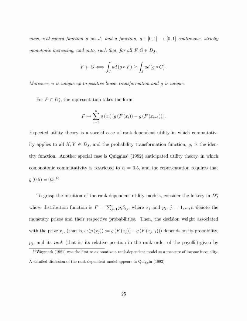
uous, real-valued function on , and a function, : [0 1] → [0 1] continuous, strictly

monotonic increasing, and onto, such that, for all ∈

< ⇐⇒Z

( ◦ ) ≥Z

( ◦)

Moreover, is unique up to positive linear transformation and is unique.

For ∈ the representation takes the form

7→X=1

() [ ( ())− ( (−1))]

Expected utility theory is a special case of rank-dependent utility in which commutativ-

ity applies to all ∈ and the probability transformation function, is the iden-

tity function. Another special case is Quiggins’ (1982) anticipated utility theory, in which

comonotonic commutativity is restricted to = 05 and the representation requires that

(05) = 0516

To grasp the intuition of the rank-dependent utility models, consider the lottery in

whose distribution function is =P

=1 where and = 1 denote the

monetary prizes and their respective probabilities. Then, the decision weight associated

with the prize (that is, ( ()) := ( ())− ( (−1))) depends on its probability,

and its rank (that is, its relative position in the rank order of the payoffs) given by

16Waymark (1981) was the first to axiomatize a rank-dependent model as a measure of income inequality.

A detailed discission of the rank dependent model appears in Quiggin (1993).

25

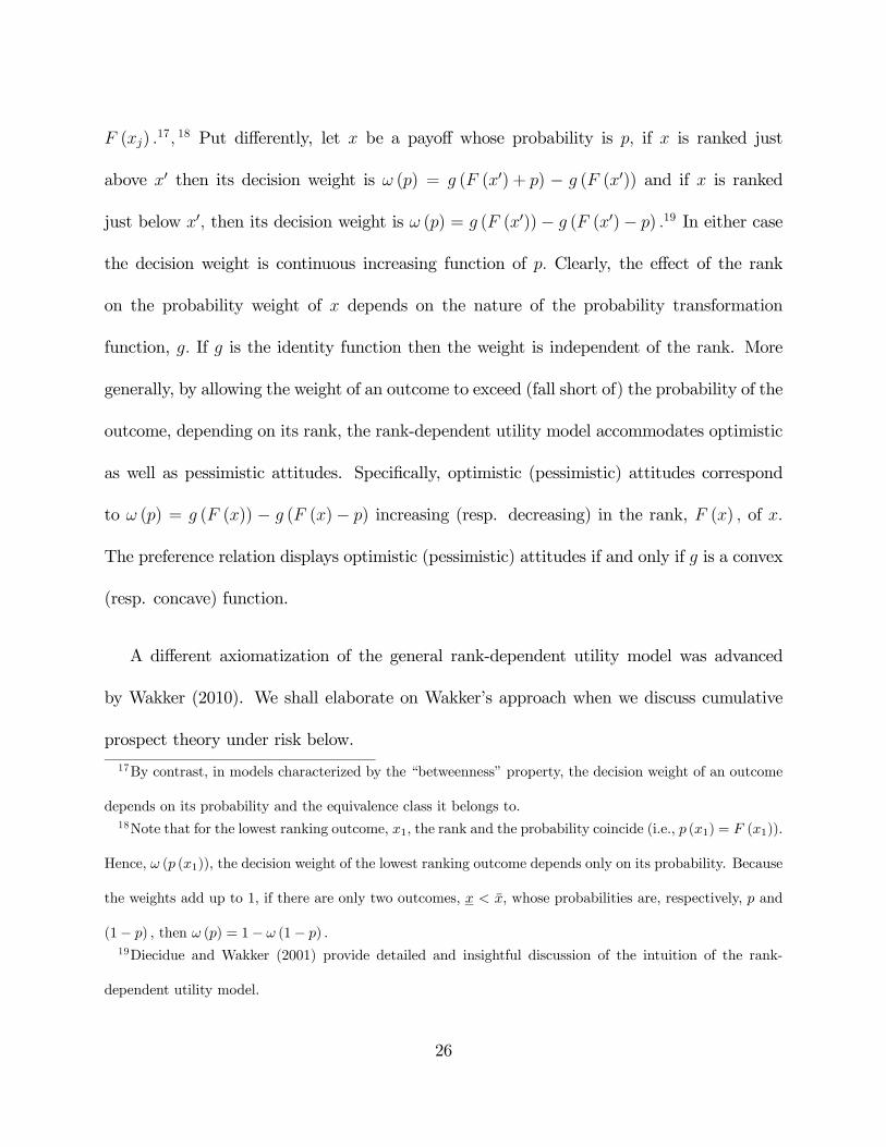
() 17 18 Put differently, let be a payoff whose probability is if is ranked just

above 0 then its decision weight is () = ( (0) + ) − ( (0)) and if is ranked

just below 0 then its decision weight is () = ( (0))− ( (0)− ) 19 In either case

the decision weight is continuous increasing function of Clearly, the effect of the rank

on the probability weight of depends on the nature of the probability transformation

function, If is the identity function then the weight is independent of the rank. More

generally, by allowing the weight of an outcome to exceed (fall short of) the probability of the

outcome, depending on its rank, the rank-dependent utility model accommodates optimistic

as well as pessimistic attitudes. Specifically, optimistic (pessimistic) attitudes correspond

to () = ( ()) − ( ()− ) increasing (resp. decreasing) in the rank, () of

The preference relation displays optimistic (pessimistic) attitudes if and only if is a convex

(resp. concave) function.

A different axiomatization of the general rank-dependent utility model was advanced

by Wakker (2010). We shall elaborate on Wakker’s approach when we discuss cumulative

prospect theory under risk below.

17By contrast, in models characterized by the “betweenness” property, the decision weight of an outcome

depends on its probability and the equivalence class it belongs to.

18Note that for the lowest ranking outcome, 1 the rank and the probability coincide (i.e., (1) = (1)).

Hence, ( (1)), the decision weight of the lowest ranking outcome depends only on its probability. Because

the weights add up to 1 if there are only two outcomes, , whose probabilities are, respectively, and

(1− ) then () = 1− (1− )

19Diecidue and Wakker (2001) provide detailed and insightful discussion of the intuition of the rank-

dependent utility model.

26

3.3 Risk attitudes and interpersonal comparisons of risk aversion

Loosely speaking, one distribution function in is more risky than another if the former is

a mean preserving spread of the latter Formally, let ∈ then is riskier than if

they have the same mean (that is,R( ()− ()) = 0) and is more dispersed than

(that is,R∩(−∞)

( ()− ()) ≥ 0 for all ). A preference relation < on is said

to exhibit risk aversion (strict risk aversion) if < ( Â ) whenever is riskier than

In expected utility theory risk attitudes are completely characterized by the properties

of the utility function. In particular, is riskier than if and only if the expected utility

of is no greater than that of for all concave utility functions. In rank-dependent util-

ity models, the attitudes towards risk depend on the properties of both the utility and the

probability transformation functions. Chew et. al. (1987) showed that individuals whose

preferences are representable by rank-dependent utility exhibit risk aversion if and only if

both the utility and the probability transformation functions are concave. Such individuals

exhibit strict risk aversion if and only if they exhibit risk aversion and either the utility func-

tion or the probability transformation function is strictly concave. Because the probability

transformation function is independent of the levels of the payoffs and variations of wealth

do not affect the rank order of the payoffs, the wealth related changes of individual attitudes

toward risk are completely characterized by the properties of the utility function. In other

words, as in expected utility theory, a preference relation exhibits decreasing (increasing,

27

constant) absolute risk aversion if and only if the utility function displays these properties

in the sense of Pratt (1964).

Unlike in expected utility theory, in the rank-dependent model the preference relation is

not smooth. Instead, it displays “kinks” at points at which the rank order of the payoffs

changes, for example, at certainty.20 At these points the preference relation exhibits first-

order risk aversion. Formally, consider the random variable + e, where e is a randomvariable whose mean is zero, denote the decision-maker’s initial wealth and ≥ 0 Let

(; e) denote the certainty equivalent of of this random variable as a function of

and (; e) = − (; e) the corresponding risk premium Clearly, (0; e) = 0Suppose that (; ; e) is twice continuously differentiable with respect to around = 0

Following Segal and Spivak (1990), a preference relation is said to exhibit first-order risk

aversion at if for every nondegenerate e (; e) |=+ 0 It is said to display

second-order risk aversion at if (; e) |=+= 0 and 2 (; e) 2 |=+ 0.

Unlike the expected utility model in which risk averse attitudes are generically second order,

risk aversion in the rank-dependent utility model is of first order. Hence, in contrast with

expected utility theory, in which risk averse decision makers take out full insurance if and

only if the insurance is fair, in the rank-dependent utility theory, risk averse decision makers

may take out full insurance even when insurance is slightly unfair.21

20In expected utility theory, risk averse attitude can only accomodate finite number of “kinks” in the

utility function. By contrast, in rank-dependent utility model the utility function may have no kinks at all

and yet, have “kinks” at points of where the rank order of the payoff changes.

21For a more elaborate discussion see also Machina (2001).

28

Given a preference relation < on and ∈ is said to differ from by a

simple compensating spread from the point of view of < if ∼ and there exist 0 ∈

such that () ≥ () for all 0 and () ≤ () for all ≥ 0 Let < and <∗

be preference relations on then < is said to exhibit greater risk aversion than <∗ if, for

all ∈ differs from by a simple compensating spread from the point of view

of < implies that <∗ If < and <∗ are representable by rank-dependent functionals

with utility and probability transformation functions ( ) and (∗ ∗) respectively, then

< exhibits greater risk aversion than <∗ if and only if ∗ and ∗ are concave transformations

of and respectively.22 The aspect of risk aversion captured by the utility function is the

same as in expected utility theory. The probability transformation function translates the

increase in spread of the underlying distribution function into spread of the decision weights.

When the probability transformation function is concave, it reduces the weights assigned to

higher ranking outcomes and increases those of lower ranking outcomes, thereby producing

a pessimistic outlook that tends to lower the overall value of the representation functional.

3.4 The dual theory

Another interesting instance of rank-dependent utility theory is Yaari’s (1987) dual theory

of choice.23 In this theory, the independence axiom is replaced with the dual-independence

axiom. To introduce the dual independence axiom consider first the set of random variables

22See Chew et. al. (1987) Theorem 1.

23See also Röell (1987).

29

V taking values in a compact interval, , in the real line The next axiom, comonotonic

independence, asserts that preference relation between two comonotonic random variables

is not reversed when each of them is amalgamated with a third random variable that is

comonotonic with both of them. Without comonotonicity, the possibility of hedging may

reverse the rank order, since decision makers who are not risk neutral are concerned with

the variability of the payoffs. Formally,

Comonotonic independence - For all pairwise comonotonic random variables, ∈

V, and all ∈ [0 1], % implies that + (1− ) % + (1− )

Comonotonic independence may be stated in terms of < on as dual independence.

Unlike the independence axiom in expected utility theory, which involves mixtures of proba-

bilities, the mixture operation that figures in the statement of dual independence is a mixture

of the comonotonic random payoffs. More concretely, the mixture operation may be por-

trayed as “portfolio mixture,” depicting the combined yield of two assets whose yields are

comonotonic. Formally, for all ∈ define the inverse function, −1 : [0 1] → by:

−1 () = sup≤{ ∈ | () = } For all ∈ and ∈ [0 1] let ⊕ (1− ) ∈

be defined by ( ⊕ (1− )) () = (−1 () + (1− )−1 ())−1 for all ∈ [0 1]

For any random variables, ∈ V, and ∈ [0 1], ⊕ (1− ) is the cumulative

distribution function of the random variable + (1− )

A preference relation % satisfies comonotonic independence if and only if the induced

30

preference relation < satisfies the dual independence axiom below.24

Dual independence - For all ∈ and ∈ [0 1] < implies that ⊕

(1− ) < ⊕ (1− )

Yaari’s (1987) dual theory representation theorem may be stated as follows:

Theorem 5: A preference relation < on satisfies weak order, continuity, monotonic-

ity and dual independence if and only if there exists a function, : [0 1]→ [0 1] continuous,

non-increasing, and onto, such that, for all ∈

< ⇐⇒Z

(1− ()) ≥Z

(1− ())

Integrating by parts, it is easy to verify that < if and only if − R (1− ()) ≥

− R (1− ()) Hence, the dual theory is the special case of the rank-dependent model

in which the utility function is linear and (1− ) = 1− () for all ∈ [0 1]

Maccheroni (2004) extended the dual theory to the case of incomplete preferences, show-

ing that the representation involves multi probability-transformation functions. Formally,

there is a set F of probability transformation functions such that, for all ∈ < if

and only if − R (1− ()) ≥ − R

(1− ()) for all ∈ F .

The expected value of cumulative distribution functions ∈ is the area of the epi-

graph of (that is, a product of the Lebesgue measures on and [0 1] of the epigraph of ).

The expected utility of is a product measure of the epigraph of , where the measure of an

24See Yaari (1987) Proposition 3.

31

interval [ ] ⊆ is given by ()− () instead of the Lebesgue measure, and the measure

on [0 1] is the Lebesgue measure. Segal (1989, 1993) axiomatized the product-measure rep-

resentation of the rank-dependent utility model. In this representation the measure on is

the same as that of expected utility but the measure of [ ] ⊆ [0 1] is given by ()− ()

4 Cumulative Prospect Theory

4.1 Introduction

Prospect theory was introduced by Kahneman and Tversky (1979) as an alternative to

expected utility theory. Intended as tractable model of decision making under risk capable

of accommodating large set of systematic violations of the expected utility model, the theory

has several special features: First, payoffs are specified in terms of gains and losses relative to

a reference point rather than as ultimate outcomes. Second, payoffs are evaluated by a real-

valued value function that is concave over gains and convex over losses and steeper for losses

than for gains, capturing a property dubbed loss aversion. Third, the probabilities of the

different outcomes are transformed using a probability weighting function which overweight

small probabilities and underweight moderate and large probabilities.25

In its original formulation the weighting function in prospect theory transformed the

probabilities of the outcomes as in equation (1) and, consequently, violates monotonicity. To

25See Tversky and Kahneman (1992).

32

overcome this difficulty, cumulative prospect theory is proposed as a synthesis of the original

prospect theory and the rank-dependent utility model.26

In what follows we present a version of cumulative prospect theory axiomatized by

Chateauneuf and Wakker (1999).

4.2 Trade-off Consistency and Representation

Consider an outcomes set whose elements are monetary rewards represented by the real

numbers. Denote by the set of prospects (that is, simple lotteries on R). Given any

= (1 1; ; ) ∈ assume that the outcomes are arranged in increasing order.27

Let < be a preference relation on Let 0 denote the payoff representing the reference point

and define the outcome as a gain if  0 and as a loss if 0 Â

Given a prospect, = (1 1 ), denote by − the prospect obtained by re-

placing the outcome in by an outcome such that +1 < < −1 (i.e., − =

(1 1; ;−1−1; ;+1 +1; ; )). Following Chateauneuf and Wakker (1999),

define a binary relation<∗ onR× R as follows: Let = (1 1; ; ), = (1 1; ; )

and such that 0 then ( ) Â∗ (0 0) if and only if − < − and −0 Â −0

and ( ) <∗ (0 0) if and only if − < − and −0 < −0. The relation <∗ rep-

resents the intensity of preference for the outcome over compared to that of 0 over 0

26See Schmidt and Zank (2009), Wakker (2010).

27More generally, the set of outcomes may be taken to be a connected topological pace and the outcomes

ranked by a complete and transitive preference relation.

33

holding the same their ranking in the prospects in which they are embedded.28 The following

axiom requires that this intensity of preferences be independent of the outcomes and their

place in the ranking in the prospects in which they are embedded.

Trade-off consistency - For no outcomes ∈ R ( ) Â∗ ( ) and ( ) <∗

( )

The following representation theorem for cumulative prospect theory is due to Chateauneuf

and Wakker (1999).

Theorem 6: A preference relation, < on satisfies weak order, continuity, monotonic-

ity and trade-off consistency if and only if there exist a continuous real-valued function,

on R, satisfying (0) = 0 and strictly increasing probability transformation functions,

+ − from [0 1] to [0 1] satisfying + (0) = − (0) = 0 and + (1) = − (1) = 1 such

that < has the following representation: For all ∈

7→X

{|≥0} ()

£+¡Σ=1

¢− +¡Σ−1=1

¢¤+

X{|≤0}

()£−¡Σ=1

¢− −¡Σ−1=1

¢¤

Note that restricted to prospects whose outcomes are either all gains or all losses, the

representation above is that of rank-dependent utility. Consequently, the rank-dependent

utility model can be axiomatized using trade-off consistency without the restrictions imposed

28Anticipating the next reult, let denote the value function of cumulative prospect theory, Chateauneuf

and Wakker (1999) showed that () Â∗ ( ) implies () − () () − () and ( ) <∗ ( )

implies ()− () ≥ ()− ()

34

by the ranks.29

Part II

Non-Expected Utility Theory Under

Uncertainty

5 Decision Problems under Uncertainty30

5.1 The decision problem

In a decision problem under uncertainty, an individual, the decision maker, considers a set

of alternative actions whose consequences depend on uncertain factors outside his control.

Formally, there is a set of available (pure) actions that can result in different (deter-

ministic) consequences , within a set , depending on which state (of nature or of the

environment) in a space obtains. For convenience, we consider finite state spaces.

29See Wakker and Tversky (1993) and Wakker (2010) .

30This and the subsequent sections are partly based on Battigalli, Cerreia-Vioglio, Maccheroni, and Mari-

nacci (2013). We refer to Gilboa and Marinacci (2013) for an alternative presentation.

35

The dependence of consequences on actions and states is described by a consequence

function

: × →

that details the consequence = ( ) of each action in each state .31 The quartet

( ) is called decision problem (under uncertainty).

Example 1 (i) Firms in a competitive market choose the level of production ∈ being

uncertain about the price ∈ that will prevail. The consequence function here is their

profit

( ) = − ()

where is the cost of producing units of good.

(ii) Players in a game choose their strategy ∈ being uncertain about the opponents’

strategy profile ∈ . Here the consequence function ( ) determines the material conse-

quences that result from strategy profile ( ).

Preferences over actions are modelled by a preorder % on . For each action ∈ , the

section of at

: →

7→ ( )

31Consequences are often called outcomes, and accordingly is called outcome function. Sometimes actions

are called decisions.

36

associates to each ∈ the consequence resulting from the choice of if obtains, and is

called Savage act induced by . In general, Savage acts are maps : → from states to

consequences. The celebrated work of Savage (1954) is based on them. In a consequentialist

perspective what matters about actions is not their label/name but the consequences that

they determine when the different states obtain.32 For this reason acts are, from a purely

methodological standpoint, the proper concept to use, so much that most of the decision

theory literature followed the Savage lead.

However, as Marschak and Radner (1972, p. 13) remark, the notions of actions, states and

implied consequences “correspond more closely to the everyday connotations of the words.”

In particular, they are especially natural in a game theoretic context, as the previous example

shows. For this reason, here we prefer to consider preferences % over in a decision problem

( ). But, in line with Savage’s insight, we postulate the following classic principle:

Consequentialism Two actions that generate the same consequence in every state are in-

different. Formally,

( ) = ( ) ∀ ∈ =⇒ ∼

or, equivalently, = =⇒ ∼ .

Under this principle, the current framework and Savage’s are essentially equivalent; see,

again, Marschak and Radner (1972, p. 13). They also show how to enrich and extend

in order to guarantee that {}∈ = . This extension is very useful for axiomatizations

32In the words of Machiavelli (1532) “si habbi nelle cose a vedere il fine e non il mezzo.”

37

and comparative statics’ exercises. For example, in this case, for each ∈ there exists a

sure action such that ( ) = for all ∈ , and this allows to set

% 0 ⇐⇒ % 0

By consequentialism, this definition is well posed. Although we will just write % 0, it is

important to keep in mind how the preference between consequences has been inferred from

that between actions. One might take the opposite perspective that decision makers have

“basic preferences” among consequences, that is, on the material outcomes of the decision

process, and these basic preferences in turn determine how they choose among actions. Be

that as it may, we regard % as describing the decision maker’s choice behavior and actions,

not consequences, are the objects of choice.

Finally, observe that % is also well defined when

= =⇒ = (2)

This assumption is not restrictive if consequentialist preferences are considered. Decision

problems satisfying it essentially correspond to reduced normal forms of games in which

realization equivalent pure strategies are merged.

We call canonical decision problem (c.d.p., for short) a decision problem ( ) in

which {}∈ = and (2) holds, so that can be seen as a “suitable index set for the set

of all acts”.33

33See Marschak and Radner (1972, p. 14). This assumption is obviously strong and Battigalli et al. (2013)

38

5.2 Mixed actions

Suppose that the decision maker can commit his actions to some random device. As a

result, he can choose mixed actions, that is, elements of the collection ∆ () of all chance34

distributions on with finite support. Pure actions can be viewed as special mixed actions:

if we denote by the Dirac measure concentrated on ∈ , we can embed in ∆ ()

through the mapping → .

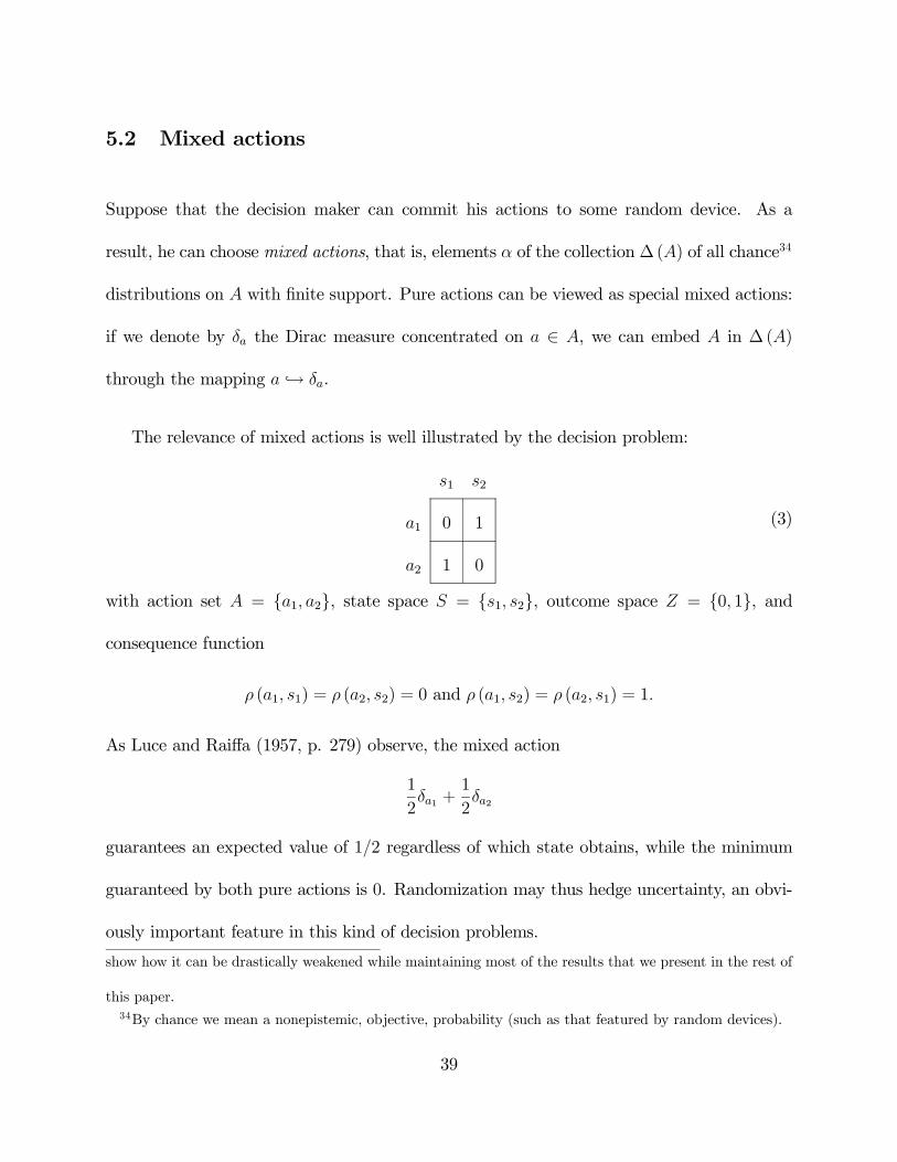
The relevance of mixed actions is well illustrated by the decision problem:

1 2

1 0 1

2 1 0

(3)

with action set = {1 2}, state space = {1 2}, outcome space = {0 1}, and

consequence function

(1 1) = (2 2) = 0 and (1 2) = (2 1) = 1

As Luce and Raiffa (1957, p. 279) observe, the mixed action

1

21 +

1

22

guarantees an expected value of 12 regardless of which state obtains, while the minimum

guaranteed by both pure actions is 0. Randomization may thus hedge uncertainty, an obvi-

ously important feature in this kind of decision problems.

show how it can be drastically weakened while maintaining most of the results that we present in the rest of

this paper.

34By chance we mean a nonepistemic, objective, probability (such as that featured by random devices).

39

Denote by ∆ () the collection of random consequences, that is, the collection of chance

distributions on with finite support. Mixed actions (chance distributions of pure actions)

induce such random consequences (chance distributions of deterministic consequences): if

the decision maker takes mixed action , the chance of obtaining consequence in state is

({ ∈ : ( ) = }) = ¡ ◦ −1 ¢ ()where is the section of at . This observation provides a natural extension of given by

: ∆ ()× → ∆ ()

( ) 7→ ◦ −1

associating to each mixed action and each state the corresponding random consequence.

Since is uniquely determined by , the hat is omitted. The domain of alternatives (and

hence of preferences %) has been extended to from pure actions to mixed actions, that is,

from to ∆ () and random consequences are implied.

In this extension, each mixed action ∈ ∆ () determines an Anscombe-Aumann act

: → ∆ ()

7→ ◦ −1

(the section of at ) that associates to each ∈ the chance distribution of consequences

resulting from the choice of if obtains. In general, Anscombe-Aumann acts are maps

: → ∆ () from states to random consequences. The analysis of Anscombe and Aumann

(1963) is based on them (which they call horse lotteries). Consequentialism naturally extends

to this mixed actions setup, with a similar motivation.

40

Chance consequentialism Two mixed actions that generate the same distribution of con-

sequences in every state are indifferent. Formally,

({ ∈ : ( ) = }) = ({ ∈ : ( ) = }) ∀ ∈ and ∈ =⇒ ∼

or, equivalently, = =⇒ ∼ .

Under this realization equivalence principle,35 a decision problem under uncertainty in

which mixed actions are available can be embedded in the Anscombe-Aumann framework, as

presented in Fishburn (1970), but with a major caveat. In such setup an act : → ∆ () is

interpreted as a non-random object of choice with random consequences (). As Fishburn

(1970, p. 176) writes

... We adopt the following pseudo-operational interpretation for ∈ ∆ (). If

is “selected” and ∈ obtains then () ∈ ∆ () is used to determine a

resultant consequence in ...

Randomization is interpreted to occur ex-post : the decision maker commits to , “ob-

serves” the realized state , then “observes” the consequence generated by the random

mechanism (), and receives .36 In contrast, the mixed actions that we consider here

35Remember that, in game theory, two mixed strategies of a player are called realization equivalent if —

for any fixed pure strategy profile of the other players — both strategies induce the same chance distribution

on the outcomes of the game. Analogously, here, two mixed actions can be called realization equivalent if —

for any fixed state — both actions induce the same chance distribution on consequences.

36We say “interpreted” since this timeline and the timed disclosure of information are unmodelled. In

41

are, by definition, random objects of choice. Randomization can be interpreted to occur

ex-ante: the decision maker commits to , “observes” the realized action , then “observes”

the realized state , and receives the consequence = ( ).37 The next simple convexity

result helps, inter alia, to understand the issue.38

Proposition 2 For each ∈ ∆ () and each ∈ [0 1],

+(1−) () = () + (1− ) () ∀ ∈

Since each mixed action can be written as a convex combination =P

∈ () of

Dirac measures, Proposition 2 implies the equality

() =X∈

() () ∀ ∈ (4)

Hence, () is the chance distribution on induced by the “ex ante” randomization of

actions with probabilities () if state obtains. Consider the act : → ∆ () given

by

() =X∈

() () ∀ ∈

Now () is the chance distribution on induced by the “ex post” randomization of

consequences ( ) with probabilities () if state obtains. But, for all ∈ , ∈ ,

principle, one could think of the decision maker committing to and receiving the outcome of the resulting

process.

37Again the timeline and the timed disclosure of information are unmodelled. In principle, one could think

of the decision maker committing to and receiving the outcome of the resulting process.

38See Battigalli et al. (2013).

42

and ∈ , denoting by (|) the chance of obtaining consequence in state if is

chosen we have

(|) = ({ ∈ : ( ) = }) =

⎧⎪⎪⎨⎪⎪⎩1 = ( )

0 otherwise

= () () (5)

That is,

() = () ∀ ( ) ∈ ×

Therefore, = since they assign the same chances to consequences in every state. Infor-

mally, they differ in the timing of randomization: decision makers “learn,” respectively, ex

ante (before “observing” the state) and ex post (after “observing” the state) the outcomes of

randomization . Whether such implementation difference matters is an empirical question

that cannot be answered in our abstract setup (or in the one of Fishburn). In a richer setup,

with two explicit layers of randomization, Anscombe and Aumann (1963, p. 201) are able

to formalize this issue and assume that “it is immaterial whether the wheel is spun before

or after the race”. Here we do not pursue this matter any more.

If ( ) is a canonical decision problem, then {}∈∆() = ∆ ().39 In particular,

since all sure actions {}∈ are available, all mixed actions with support in this set are

available too. A special feature of these actions is that the chance distribution of conse-

quences they generate do not depend on the realized state. For this reason, we call them

39But notice that the reduction assumption (2) does not imply that = if = when and are

mixed actions. In the simple canonical decision problem (11), for example, = 12+

12 and =

12+

12

have disjoint support, but = . See also Battigalli et al. (2013).

43

lottery actions and denote ∆ () =© ∈ ∆ () : supp ⊆ {}∈

ªthe set of all of them.

Setting

=X∈

() ∀ ∈ ∆ ()

the correspondence → is actually an affine embedding of ∆ () onto ∆ () such that,

for each ∈ ,

() =X

∈supp () () =

X∈supp

() ( ) =X

∈supp () =

This embedding allows to identify ∆ () and ∆ (), and so to set

%∆() 0 ⇐⇒ % 0

for 0 ∈ ∆ (). In view of this we can write ∈ ∆ ().

5.3 Subjective expected utility

The theory of decisions under uncertainty investigates the preferences’ structures underlying

the choice criteria that decision makers use to rank alternatives in a decision problem. In

our setting, this translates in the study of the relations between the properties of preferences

% on ∆ () and those of preference functionals which represent them, that is, functionals

: ∆ ()→ R such that

% ⇐⇒ () ≥ ()

The basic preference functional is the subjective expected utility one, axiomatized by Savage

(1954); we devote this section to the version of Savage’s representation due to Anscombe

and Aumann (1963).

44

Definition 3 Let ( ) be a c.d.p., a binary relation % on ∆ () is a rational prefer-

ence (under uncertainty) if it is:

1. reflexive: = implies ∼ ;

2. transitive: % and % implies % ;

3. monotone: () %∆() () for all ∈ implies % .

The latter condition is a preferential version of consequentialism: if the random conse-

quence generated by is preferred to the random consequence generated by irrespectively

of the state, then is preferred to .

Proposition 4 Let ( ) be a c.d.p. and % be a rational preference on ∆ (), then %

satisfies chance consequentialism.

Proof. If ∈ ∆ () and () = () for all ∈ , then () = (), reflexivity

implies () ∼ (). But then () ∼∆() () for all ∈ by the definition of %∆()

and monotonicity delivers ∼ . ¥

Next we turn to a basic condition about decision makers’ information.

Completeness For all ∈ ∆ (), it holds % or % .

Completeness thus requires that decision makers be able to compare any two alternatives.

We interpret it as a statement about the quality of decision makers’ information, which

45

enables them to make such comparisons, rather than about their decisiveness. Although it

greatly simplifies the analysis, it is a condition conceptually less compelling than transitivity

and monotonicity (see Section 7.1).

Next we state a standard regularity condition, due to Herstein and Milnor (1953).

Continuity The sets { ∈ [0 1] : + (1− ) % } and { ∈ [0 1] : % + (1− )}

are closed for all ∈ ∆ ().

The last key ingredient is the independence axiom. Formally,

Independence If ∈ ∆ (), then

∼ =⇒ 1

2+

1

2 ∼ 1

2 +

1

2.

This classical axiom requires that mixing with a common alternative does not alter the

original ranking of two mixed actions. When restricted to ∆ () ' ∆ () it reduces to

the von Neumann-Morgenstern original independence axiom on lotteries. Notice that the

independence axiom implies indifference to randomization, that is,

∼ =⇒ 1

2+

1

2 ∼ (6)

In fact, by setting = , the axiom yields

∼ =⇒ 1

2+

1

2 ∼ 1

2 +

1

2 =

This key feature of independence will be questioned in the next section by the Ellsberg

paradox.

46

The previous preferential assumptions lead to the Anscombe and Aumann (1963) version

of Savage’s result.

Theorem 7: Let ( ) be a c.d.p. and % be a binary relation on ∆ (). The

following conditions are equivalent:

1. % is a nontrivial, complete, and continuous rational preference that satisfies indepen-

dence;

2. there exist a nonconstant : → R and a probability distribution ∈ ∆ () such

that the preference functional

() =X

()

ÃX

() ( ( ))

!(7)

represents % on ∆ ().

The function is cardinally unique40 and is unique.

To derive this version of the Anscombe-Aumann representation based on actions from the

more standard one based on acts (see Schmeidler, 1989, p. 578), notice that by Proposition

2 the map

: ∆ () → ∆ ()

7→

is affine and onto (since the decision problem is canonical). Chance consequentialism of %

(implied by Proposition 4) allows to derive % on ∆ ()by setting, for = () and

40That is, unique up to an affine strictly increasing transformation.

47

= () in ,

% ⇐⇒ %

By affinity of , we can transfer to % all the assumptions we made on %. This takes us

back to the standard Anscombe-Aumann setup.41

The embedding → of pure actions into mixed actions allows to define

% ⇐⇒ %

Thus (7) implies

% ⇐⇒X

() ( ( )) ≥X

() ( ( )) (8)

which is the subjective expected utility representation of Marschak and Radner (1972, p.

16). The function is a utility function since (8) implies

% 0 ⇐⇒ () ≥ (0)

Following the classic insights of Ramsey (1926) and de Finetti (1931, 1937), rankings of bets

on events can be used to elicit the decision maker’s subjective assessment of their likelihoods.

To this end, denote by 0 ∈ the bet on event ⊆ that delivers if obtains and 0

otherwise, with 0 ≺ . By (8),

0 % 00 ⇐⇒ () ≥ (0)

and so can be regarded as a subjective probability.

41More on the relation between the mixed actions setup we adopt here and the standard Anscombe-

Aumann setup can be found in Battigalli et al. (2013).

48

Eachmixed action generates, along with the subjective probability ∈ ∆ (), a product

probability distribution × ∈ ∆ (× ). Since

X

()

ÃX

() ( ( ))

!=

X()∈×

( ( )) () () = E× ( ◦ )

we can rewrite (7) as follows

() = E× ( ◦ ) (9)

In this perspective, () is the expected payoff of the mixed action profile ( ) for the

decision maker in a game ({} {} { ◦ ◦ }) in which the decision maker

chooses mixed strategy and nature (denoted by and assumed to determine the state of

the environment) chooses mixed strategy . But notice that, while is a chance distribution

available to the decision maker, is a subjective belief of the decision maker on nature’s

behavior.

6 Uncertainty Aversion: Definition and Representa-

tion

6.1 The Ellsberg paradox

Consider a coin that a decision maker knows to be fair, as well as an urn that he knows to

contain 100 black and white balls in unknown ratio: there may be from 0 to 100 black balls.42

42A fair coin here is just a random device generating two outcomes with the same 12 chance. The original

paper of Ellsberg (1961) models it through another urn that the decision maker knows to contain 50 white

49

To bet on heads/tails means that the decision maker wins $100 if the tossed coin lands on

heads/tails (and nothing otherwise); similarly, to bet on black/white means that the decision

maker wins $100 if a ball drawn from the urn is black/white (and nothing otherwise).

Ellsberg’s (1961) thought experiment suggests, and a number of behavioral experiments

confirm, that many decision makers are indifferent between betting on either heads or tails

and are also indifferent between betting on either black or white, but they strictly prefer to

bet on the coin rather than on the urn. We can represent this preference pattern as

bet on white ∼ bet on black ≺ bet on heads ∼ bet on tails (10)

To understand the pattern, notice that the decision maker has a much better information

to assess the likelihood of the outcome of the coin toss than of the urn draw. In fact,

the likelihood of the coin toss is quantified by chance, it is an objective (nonepistemic)

probability, here equal to 12; in contrast, the decision maker has to assess the likelihood

of the urn draw by a subjective (epistemic) probability, based on essentially no information

since the urn’s composition is unknown.

balls and 50 black balls.

50

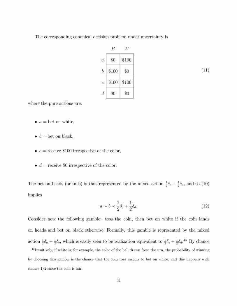
The corresponding canonical decision problem under uncertainty is

$0 $100

$100 $0

$100 $100

$0 $0

(11)

where the pure actions are:

• = bet on white,

• = bet on black,

• = receive $100 irrespective of the color,

• = receive $0 irrespective of the color.

The bet on heads (or tails) is thus represented by the mixed action 12 +

12, and so (10)

implies

∼ ≺ 12 +

1

2 (12)

Consider now the following gamble: toss the coin, then bet on white if the coin lands

on heads and bet on black otherwise. Formally, this gamble is represented by the mixed

action 12 +

12, which is easily seen to be realization equivalent to

12 +

12.

43 By chance

43Intuitively, if white is, for example, the color of the ball drawn from the urn, the probability of winning

by choosing this gamble is the chance that the coin toss assigns to bet on white, and this happens with

chance 12 since the coin is fair.

51

consequentialism, (12) therefore implies

∼ ≺ 12 +

1

2 (13)

which violates (6), and so subjective expected utility maximization.

It is important to observe that such violation, and the resulting preference for randomiza-

tion, is normatively compelling: randomization eliminates the dependence of the probability

of winning on the unknown composition of the urn, and makes this probability a chance, thus

hedging uncertainty. As observed at the beginning of Section 5.2, the mixed action 12+

12

guarantees an expected value of $50 regardless of which state obtains, while the minimum

guaranteed (expected value) by both pure actions is $0 (although the maximum is $100).

Preference pattern (13) is not the result of a bounded rationality issue: the Ellsberg paradox

points out a normative inadequacy of subjective expected utility, which ignores a hedging

motif that decision makers may deem relevant because of the quality of their information. In

what follows, we call ambiguity the type of information/uncertainty that makes such motif

relevant.44

44A caveat: in our setup randomization plays a major role and, accordingly, we are considering the Ellsberg

paradox from this angle. However, as Gilboa and Marinacci (2013) discuss, the paradox continues to hold

even without randomization as it entails a normatively compelling violation of Savage’s sure thing principle.

52

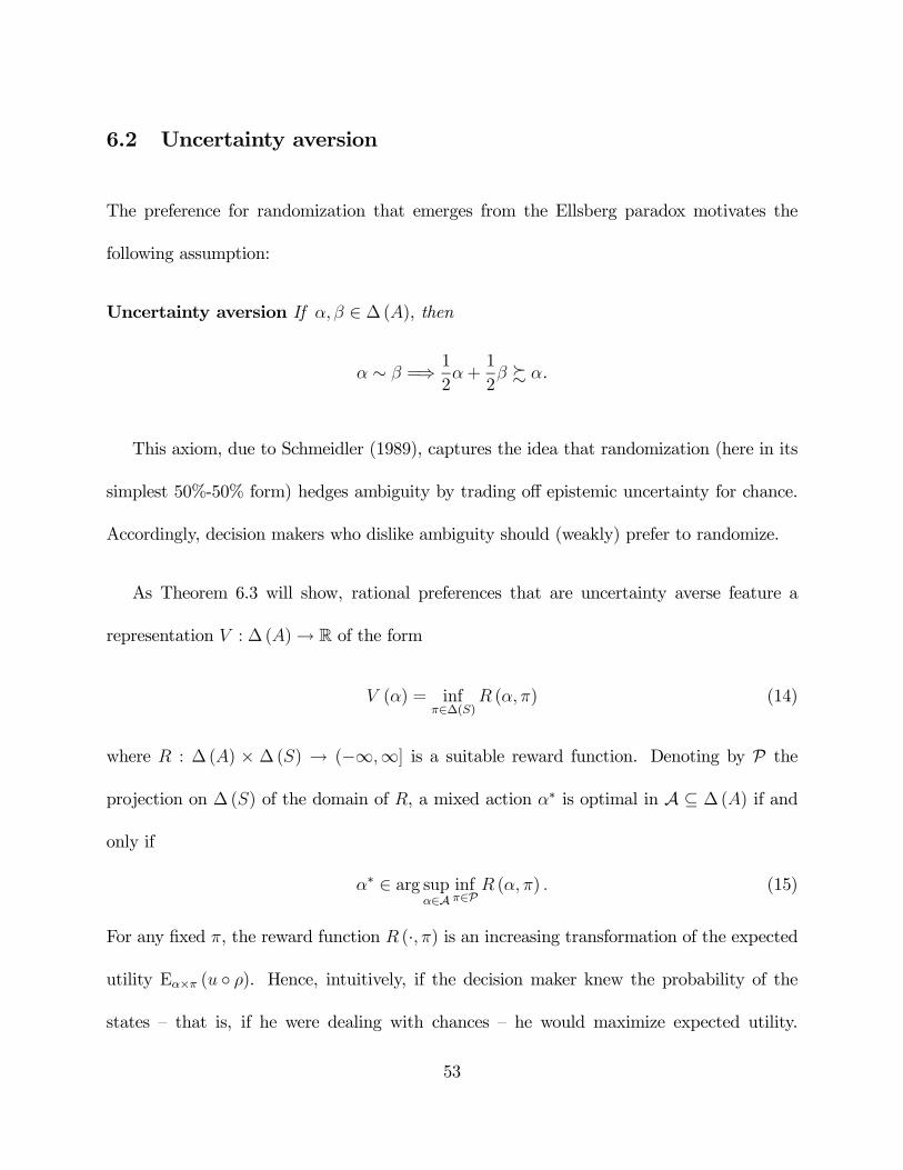
6.2 Uncertainty aversion

The preference for randomization that emerges from the Ellsberg paradox motivates the

following assumption:

Uncertainty aversion If ∈ ∆ (), then

∼ =⇒ 1

2+

1

2 % .

This axiom, due to Schmeidler (1989), captures the idea that randomization (here in its

simplest 50%-50% form) hedges ambiguity by trading off epistemic uncertainty for chance.

Accordingly, decision makers who dislike ambiguity should (weakly) prefer to randomize.

As Theorem 6.3 will show, rational preferences that are uncertainty averse feature a

representation : ∆ ()→ R of the form

() = inf∈∆()

( ) (14)

where : ∆ () × ∆ () → (−∞∞] is a suitable reward function. Denoting by P the

projection on ∆ () of the domain of , a mixed action ∗ is optimal in A ⊆ ∆ () if and

only if

∗ ∈ arg sup∈A

inf∈P

( ) (15)

For any fixed , the reward function (· ) is an increasing transformation of the expected

utility E× ( ◦ ). Hence, intuitively, if the decision maker knew the probability of the

states — that is, if he were dealing with chances — he would maximize expected utility.

53

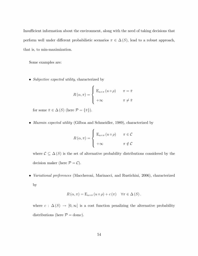
Insufficient information about the environment, along with the need of taking decisions that

perform well under different probabilistic scenarios ∈ ∆ (), lead to a robust approach,

that is, to min-maximization.

Some examples are:

• Subjective expected utility, characterized by

( ) =

⎧⎪⎪⎨⎪⎪⎩E× ( ◦ ) =

+∞ 6=

for some ∈ ∆ () (here P = {}).

• Maxmin expected utility (Gilboa and Schmeidler, 1989), characterized by

( ) =

⎧⎪⎪⎨⎪⎪⎩E× ( ◦ ) ∈ C

+∞ ∈ C

where C ⊆ ∆ () is the set of alternative probability distributions considered by the

decision maker (here P = C).

• Variational preferences (Maccheroni, Marinacci, and Rustichini, 2006), characterized

by

( ) = E× ( ◦ ) + () ∀ ∈ ∆ ()

where : ∆ () → [0∞] is a cost function penalizing the alternative probability

distributions (here P = dom).

54

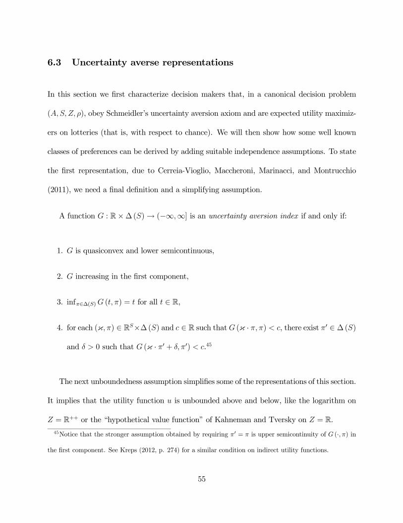
6.3 Uncertainty averse representations

In this section we first characterize decision makers that, in a canonical decision problem

( ), obey Schmeidler’s uncertainty aversion axiom and are expected utility maximiz-

ers on lotteries (that is, with respect to chance). We will then show how some well known

classes of preferences can be derived by adding suitable independence assumptions. To state

the first representation, due to Cerreia-Vioglio, Maccheroni, Marinacci, and Montrucchio

(2011), we need a final definition and a simplifying assumption.

A function : R×∆ ()→ (−∞∞] is an uncertainty aversion index if and only if:

1. is quasiconvex and lower semicontinuous,

2. increasing in the first component,

3. inf∈∆() ( ) = for all ∈ R,

4. for each (κ ) ∈ R×∆ () and ∈ R such that (κ · ) , there exist 0 ∈ ∆ ()

and 0 such that (κ · 0 + 0) .45

The next unboundedness assumption simplifies some of the representations of this section.

It implies that the utility function is unbounded above and below, like the logarithm on

= R++ or the “hypothetical value function” of Kahneman and Tversky on = R.

45Notice that the stronger assumption obtained by requiring 0 = is upper semicontinuity of (· ) in

the first component. See Kreps (2012, p. 274) for a similar condition on indirect utility functions.

55

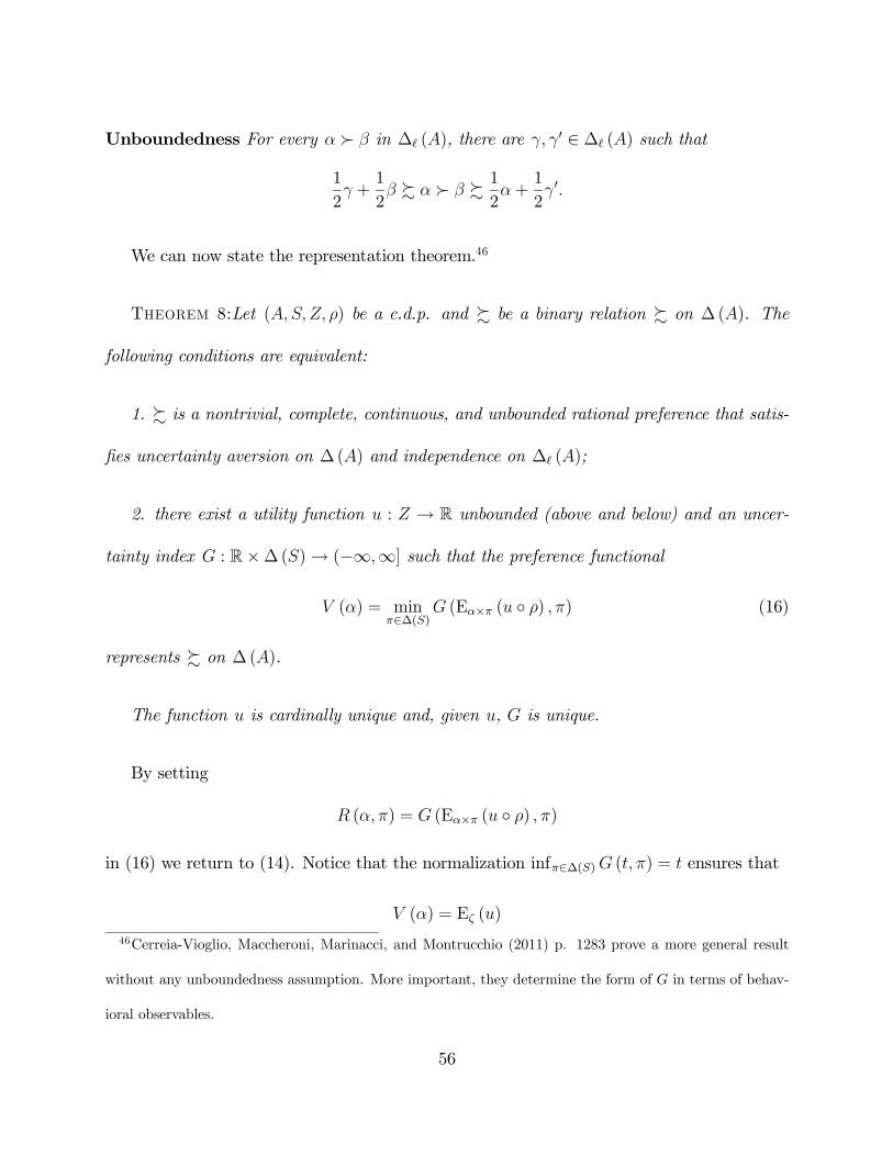
Unboundedness For every  in ∆ (), there are 0 ∈ ∆ () such that

1

2 +

1

2 % Â % 1

2+

1

20

We can now state the representation theorem.46

Theorem 8:Let ( ) be a c.d.p. and % be a binary relation % on ∆ (). The

following conditions are equivalent:

1. % is a nontrivial, complete, continuous, and unbounded rational preference that satis-

fies uncertainty aversion on ∆ () and independence on ∆ ();

2. there exist a utility function : → R unbounded (above and below) and an uncer-

tainty index : R×∆ ()→ (−∞∞] such that the preference functional

() = min∈∆()

(E× ( ◦ ) ) (16)

represents % on ∆ ().

The function is cardinally unique and, given , is unique.

By setting

( ) = (E× ( ◦ ) )

in (16) we return to (14). Notice that the normalization inf∈∆() ( ) = ensures that

() = E ()

46Cerreia-Vioglio, Maccheroni, Marinacci, and Montrucchio (2011) p. 1283 prove a more general result

without any unboundedness assumption. More important, they determine the form of in terms of behav-

ioral observables.

56

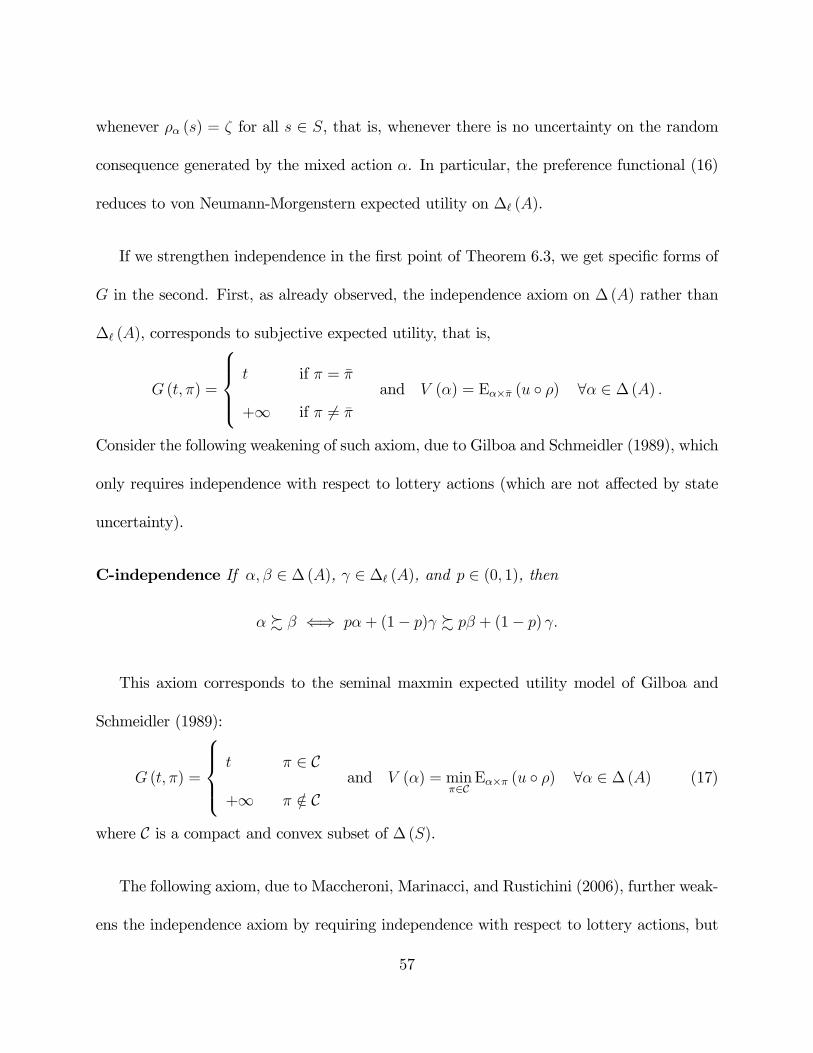
whenever () = for all ∈ , that is, whenever there is no uncertainty on the random

consequence generated by the mixed action . In particular, the preference functional (16)

reduces to von Neumann-Morgenstern expected utility on ∆ ().

If we strengthen independence in the first point of Theorem 6.3, we get specific forms of

in the second. First, as already observed, the independence axiom on ∆ () rather than

∆ (), corresponds to subjective expected utility, that is,

( ) =

⎧⎪⎪⎨⎪⎪⎩ if =

+∞ if 6=

and () = E× ( ◦ ) ∀ ∈ ∆ ()

Consider the following weakening of such axiom, due to Gilboa and Schmeidler (1989), which

only requires independence with respect to lottery actions (which are not affected by state

uncertainty).

C-independence If ∈ ∆ (), ∈ ∆ (), and ∈ (0 1), then

% ⇐⇒ + (1− ) % + (1− )

This axiom corresponds to the seminal maxmin expected utility model of Gilboa and

Schmeidler (1989):

( ) =

⎧⎪⎪⎨⎪⎪⎩ ∈ C

+∞ ∈ Cand () = min

∈CE× ( ◦ ) ∀ ∈ ∆ () (17)

where C is a compact and convex subset of ∆ ().

The following axiom, due to Maccheroni, Marinacci, and Rustichini (2006), further weak-

ens the independence axiom by requiring independence with respect to lottery actions, but

57

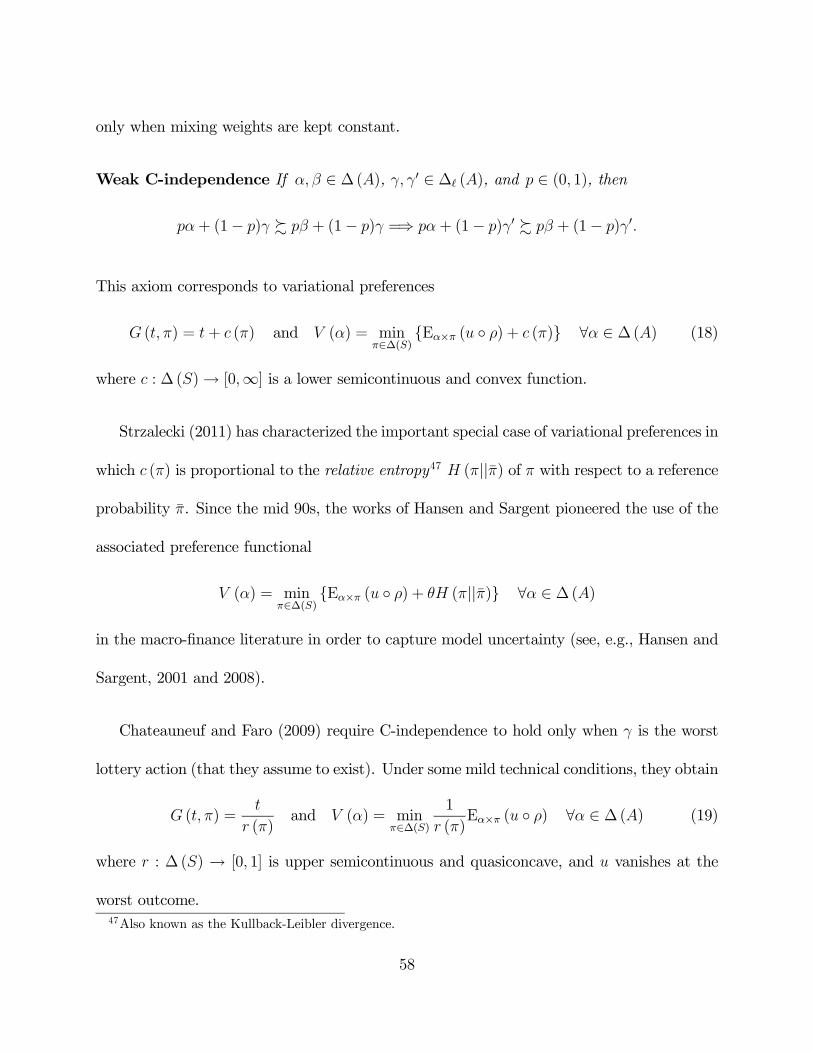
only when mixing weights are kept constant.

Weak C-independence If ∈ ∆ (), 0 ∈ ∆ (), and ∈ (0 1), then

+ (1− ) % + (1− ) =⇒ + (1− )0 % + (1− )0

This axiom corresponds to variational preferences

( ) = + () and () = min∈∆()

{E× ( ◦ ) + ()} ∀ ∈ ∆ () (18)

where : ∆ ()→ [0∞] is a lower semicontinuous and convex function.

Strzalecki (2011) has characterized the important special case of variational preferences in

which () is proportional to the relative entropy47 (||) of with respect to a reference

probability . Since the mid 90s, the works of Hansen and Sargent pioneered the use of the

associated preference functional

() = min∈∆()

{E× ( ◦ ) + (||)} ∀ ∈ ∆ ()

in the macro-finance literature in order to capture model uncertainty (see, e.g., Hansen and

Sargent, 2001 and 2008).

Chateauneuf and Faro (2009) require C-independence to hold only when is the worst

lottery action (that they assume to exist). Under some mild technical conditions, they obtain

( ) =

()and () = min

∈∆()1

()E× ( ◦ ) ∀ ∈ ∆ () (19)

where : ∆ () → [0 1] is upper semicontinuous and quasiconcave, and vanishes at the

worst outcome.47Also known as the Kullback-Leibler divergence.

58

7 Beyond Uncertainty Aversion

The uncertainty averse models that we just reviewed originate in Schmeidler (1989). For our

setup is especially relevant his insight about preference for randomization as an hedge toward

ambiguity. We now present two different approaches toward ambiguity, due to Bewley (1986)

and Klibanoff, Marinacci and Mukerji (2005), that do not rely on this assumption.

7.1 Incompleteness

Completeness of preferences requires that decision makers have enough information to rank

all mixed actions. Under uncertainty, however, decision makers might well lack this infor-

mation so that they might be unable to compare some pairs of alternatives.

This motivated Truman Bewley to present in 1986 a model of choice under uncertainty

that restricts completeness to the set of lotteries alone; these alternatives induce a chance

distribution that do not depend on states and so are not affected by epistemic uncertainty.

Gilboa, Maccheroni, Marinacci, and Schmeidler (2010) established the following form of

Bewley’s representation theorem.48

Theorem 9:Let ( ) be a c.d.p. and % be a binary relation % on ∆ (). The

following conditions are equivalent:

48Relative to the original version, this version of the theorem uses a weak preference % rather than a strict

one  and remains true also when is infinite.

59

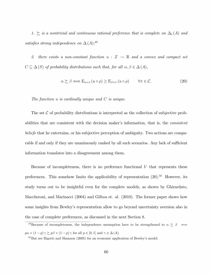
1. % is a nontrivial and continuous rational preference that is complete on ∆ () and

satisfies strong independence on ∆ ();49

2. there exists a non-constant function : → R and a convex and compact set

⊆ ∆ () of probability distributions such that, for all ∈ ∆ (),

% ⇐⇒ E× ( ◦ ) ≥ E× ( ◦ ) ∀ ∈ C (20)

The function is cardinally unique and is unique.

The set C of probability distributions is interpreted as the collection of subjective prob-

abilities that are consistent with the decision maker’s information, that is, the consistent

beliefs that he entertains, or his subjective perception of ambiguity. Two actions are compa-

rable if and only if they are unanimously ranked by all such scenarios. Any lack of sufficient

information translates into a disagreement among them.

Because of incompleteness, there is no preference functional that represents these

preferences. This somehow limits the applicability of representation (20).50 However, its

study turns out to be insightful even for the complete models, as shown by Ghirardato,

Maccheroni, and Marinacci (2004) and Gilboa et. al. (2010). The former paper shows how

some insights from Bewley’s representation allow to go beyond uncertainty aversion also in

the case of complete preferences, as discussed in the next Section 8.

49Because of incompleteness, the independence assumption have to be strengthened to % ⇐⇒

+ (1− ) % + (1− ) for all ∈ [0 1] and ∈ ∆ ().50But see Rigotti and Shannon (2005) for an economic application of Bewley’s model.

60

Gilboa et. al. (2010) noted that, although decisions eventually have to be made, in

many decision problems preferences that can be intersubjectively justified are incomplete.

For this reason they proposed a model based on two preference relations, one incomplete a

la Bewley and one complete a la Gilboa and Schmeidler (1989). They showed that under

certain axioms, stated on each preference relation separately as well as relating the two, they

are jointly represented by the same set of probabilities C: one via the unanimity rule (20),

and the other via the maxmin rule (17). This shows how maxmin expected utility behavior

may result from incomplete preferences.

Further results on incompleteness in a decision problem under uncertainty appear in

Ghirardato, Maccheroni, Marinacci, Siniscalchi (2003), Ok, Ortoleva and Riella (2012), and

Galaabaatar and Karni (2012).

7.2 Smooth ambiguity model

The models presented in the previous section of the form

() = inf∈∆()

( ) (21)

are often viewed as rather extreme, almost paranoid, since they evaluate through the

worst values in the range of rewards { ( ) | ∈ ∆ ()}. Indeed, (21) reminds Wald’s

(1950) interpretation of a decision problem under uncertainty as a zero-sum game against (a

malevolent) nature.51

51But remember that, as observed, subjective expected utility is a special case of this representation.

61

However, the reward function ( ) incorporates both the attitude toward ambiguity,

a taste component, and its perception, an information component. To fix ideas, consider

a maxmin expected utility preference that features a set C of subjective probabilities. A

smaller set C may reflect both better information — that is, a lower perception of ambiguity

— and/or a less averse uncertainty attitude. In other words, the size of C does not reflect just

information, but taste as well.52

The criterion (21) is thus not extreme; indeed, the axioms underlying it (that we have

seen above) are not extreme at all.53 That said, many economic applications that use such

criterion regard the set C — and more generally the projection on ∆ () of the domain of

— as being essentially determined by information, that is, as the set of probabilities that are

consistent with objectively available information. As such, the elements of C are basically

viewed as chance distributions, typically data generating processes in the macro-finance

applications. For example, in the Ellsberg paradox the set C for the unknown urn consists of

all chance distributions determined by the possible compositions of the urn (hence C = ∆ ()

when there is no information about such compositions).

Under this “chance” interpretation of C, criterion (21) is quite extreme and loses some of

its appeal. Klibanoff, Marinacci, and Mukerji (2005) proposed a different model that tries

to address this issue. They assume that decision makers have a subjective probability over

52See Gajdos, Hayashi, Tallon, and Vergnaud (2008) for a model that explicitly relates C with some

underlying objective information.

53Notice that if ( ) = +∞ for all then is never considered in minimization (21).

62

the (Borel) set C ⊆ ∆ () of all possible chance distributions. Via reduction, the (prior)

probability determines a (predictive) probability =R∆()

() on . The subjective

expected utility criterion can be rewritten as:Z∆()

(E× ( ◦ )) () = E× ( ◦ ) (22)

Decision makers, however, may well dislike the uncertainty about the expected payoffE× ( ◦ ),

while criterion (22) just averages out these payoffs, tacitly assuming a neutral attitude to-

wards this kind of uncertainty. If, in contrast, ambiguity aversion (or propension) prevails

(as one expects to be usually the case), a nonlinear function : co () → R should be

introduced to capture it.54 Criterion (22) then generalizes to

() =

Z∆()

(E× ( ◦ )) () (23)

Note that we have a separation between the uncertainty perception, an information feature

modelled by and its support C, and the uncertainty attitude, a taste trait modelled by

and its shape. In particular, the concavity of corresponds to a ambiguity aversion.

Criterion (23), due to Klibanoff et. al. (2005), has become to be known as the smooth

model of ambiguity because, under mild assumptions, is a smooth functional (whereas the

maxmin expected utility functionals are typically not everywhere differentiable). Related

models have been proposed by Segal (1987), Neilson (1993), Nau (2006), Ergin and Gul

(2009), and Seo (2009).

A main feature of the smooth model is the ability to take advantage of conventional

54See also Section 8.2 below. Here co () denotes the smallest interval that contains ().

63

risk theory in studying ambiguity attitudes, something that makes it especially tractable.55

Moreover, if the concavity of becomes stronger and stronger, reflecting greater and greater

uncertainty aversion, it can be shown that criterion (23) tends to the maxmin expected

utility criterion

inf∈supp

E× ( ◦ )

which can thus be regarded as a limit case of the smooth model.

8 Alternative Approaches

The models presented in the previous Section 7 depart from uncertainty aversion in a rad-

ical way: removing completeness or taking a neo-Bayesian “prior-over-models” approach.

It is natural to wonder whether the uncertainty averse models of Section 6.3 can be just

generalized beyond uncertainty aversion thus encompassing more general attitudes.

Ghirardato, Maccheroni and Marinacci (2004),56 investigated this issue by considering

a complete, continuous, and nontrivial rational preference % on ∆ () that satisfies the

55In this regard, Maccheroni, Marinacci, and Ruffino (2013) established a quadratic approximation of

criterion (23) that extends the classic expected utility results of de Finetti (1952), Pratt (1964), and Arrow

(1965). On these classic results see Montesano (2009).

56Recently extended by Cerreia-Vioglio, Maccheroni, Marinacci, and Siniscalchi (2011), and by Ghirardato

and Siniscalchi (2012).

64

independence axiom on ∆ (), and its subrelation

%∗ ⇐⇒ + (1− ) % + (1− ) ∀ ∈ [0 1] and ∈ ∆ ()

We have %∗ when the decision maker does not find any possibility of hedging against or

speculating on the ambiguity that the comparison of the two mixed actions involves. If so,

Ghirardato et. al. (2004) argue that such ambiguity does not affect the preference among

them; for this reason they call %∗ the “unambiguous preference.”

Because of ambiguity,%∗ is in general not complete. It is rational and satisfies the (strong)

independence axiom, so that it admits a unanimity representation (20). An incomplete

preference a la Bewley thus emerges in studying very general preferences, with an associated

utility and consistent beliefs given by a “Bewley set” C of probability distributions.57 The

consistency between beliefs and behavior is confirmed by the possibility of representing the

original preference % by a functional

() = ()min∈C

E× ( ◦ ) + (1− ())max∈C

E× ( ◦ )

where the maximum and the minimum expected utilities of are weighted in the evaluation.

This representation provides a separation between the revealed perception of ambiguity

embodied by the set C, and the decision maker reaction to it when evaluating captured by

().

57Notably for maxmin expected utility preferences C is exactly the set over which the minimum is taken.

We also remark that, in the original setting Ghirardato et al. (2004) assume C-independence of %, but

Cerreia-Vioglio et al. (2011) show how this assumption is redundant for this part of the analysis.

65

See Amarante (2009) and Eichberger, Grant, Kelsey, and Koshevoy (2011) for further

insights on this approach.

8.1 Choquet expected utility

The first axiomatic model of choice under ambiguity appears in the seminal paper of Schmei-

dler (1989) on Choquet expected utility.58 The implied preferences are a special subclass of

those considered by Ghirardato et. al. (2004). The crucial axiom here is the comonotonic

independence axiom, that is a stronger version of C-independence.

Extending the definition of comonotonic random variables (given in the first part of this

article), say that mixed actions ∈ ∆ () are comonotonic if it is never the case that

both ( ) Â ( 0) and ( ) ≺ ( 0) for some states and 0. As in the case of

random variables, the convex combination of comonotonic mixed actions cannot provide any

hedging.

Comonotonic independence If ∈ ∆ () are pairwise comonotonic and 0 1,

then  implies + (1− )  + (1− ).

Schmeidler (1989) proved a representation theorem for rational preferences that satisfy

this axiom. Call capacity (or nonadditive probability) a set function : 2 → [0 1] such that

1. (∅) = 0 and () = 1;

58For axiomatizations without randomization see Gilboa (1985) and Chew and Karni (1994).

66

2. ⊆ 0 implies () ≤ (0).

Expectations E with respect to can be computed via the Choquet integral, named

after Choquet (1953) and they coincide with standard expectations when is additive (that

is a probability distribution).59

We can now state Schmeidler’s famous result.

Theorem 10:Let ( ) be a c.d.p. and % be a binary relation % on ∆ (). The

following conditions are equivalent:

1. % is a nontrivial, complete, and continuous rational preference that satisfies comonotonic

independence;

2. there exists a nonconstant : → R and a capacity : 2 → [0 1] such that the

preference functional

() = E [E ( ◦ )]

represents % on ∆ ().

The function is cardinally unique and the capacity is unique.

In particular, in the first point, the full-fledged independence axiom holds if and only

59We refer to Gilboa and Marinacci (2011) for an introduction to Choquet integration, and to Schmeidler

(1986), Denneberg (1994) and Marinacci and Montrucchio (2004) for more detailed studies. Ryan (2009)

presents a simple pedagogical proof in the finite state case of the Schmeidler Theorem (and of other ambiguity

representations).

67

if is additive. In this case, we return to subjective expected utility. More interestingly,

Schmeidler (1989) shows that in the previous theorem the preference % satisfies uncertainty

aversion if and only if the capacity is supermodular

( ∪0) + ( ∩ 0) ≥ () + (0) ∀0 ⊆

In this case,

E [E ( ◦ )] = min∈core()

E× ( ◦ )

where core (), called the core of , is the set of probability distributions determined by

as follows:60

core () = { ∈ ∆ () : () ≥ () for all ⊆ }

Uncertainty aversion thus characterizes the overlap among Choquet expected utility and

maxmin expected utility, and in this case the set of consistent beliefs (representing %∗) is

C = core ().

Noticeably, in the special case in which ⊆ R+, is the identity, and = ◦ for some

∈ ∆ () and some increasing : [0 1]→ [0 1], then

() =

Z ∞

0

(1− ( ∈ : () ≤ )) ∀ ∈

thus obtaining Yaari’s (1987) dual theory representation. Another tractable representation,

due to Chateauneuf, Eichberger, and Grant (2007), is the so called neo-additive Choquet

60Mathematically, capacities are a special class of transferable utility games (see Marinacci and Montruc-

chio, 2004, for some details on this observation). The notion of core here is adapted from the the game

theoretic one.

68

expected utility model of the “Hurwicz”form

() = (1− − ) E [E ( ◦ )] + min∈

E ( ◦ ) + max∈

E ( ◦ )

Through the values of the weights and , the preference functional captures in a simple

way different degrees of pessimism and optimism.

8.2 Uncertainty aversion revisited

Schmeidler’s uncertainty aversion axiom models ambiguity aversion through preference for

randomization. As such, it crucially relies on the presence of randomization. But, ambi-

guity is a feature of an information state that may occur whether or not randomization is

available. This led Epstein (1999) and Ghirardato and Marinacci (2002) to address ambigu-

ity/uncertainty aversion from a different angle, inspired by the comparative analysis of risk

attitudes of Yaari (1969).

Although our setup features randomization, their works still shed light on some notewor-

thy aspects of ambiguity aversion. Specifically, the approach of Ghirardato and Marinacci

(2002), which we present here because of its sharper model implications, relies on two basic

ingredients:

1. A comparative notion of ambiguity aversion that, given any two preferences %1 and

%2 on ∆ (), says when %1 is more ambiguity averse than %2.

69

2. A benchmark for neutrality to ambiguity; that is, a class of preferences % on ∆ ()

that are viewed as neutral to ambiguity.

In turn, the choice of these ingredients determines the absolute notion of ambiguity

aversion: a preference % is classified as ambiguity averse provided that it is more ambiguity

averse than an ambiguity neutral one.

The first ingredient, the comparative notion, is based on the comparison of mixed actions

with lottery ones. Specifically, we say that %1 is more ambiguity averse than %2 if, for all

∈ ∆ () and all ∈ ∆ (),

%1 =⇒ %2

Lottery actions are unaffected by state uncertainty and so are definitely unambiguous alter-

natives (whatever meaning we attach to such adjective). Any other mixed action may only

embody equal or more ambiguity than them. The definition above ranks ambiguity attitudes

by calling decision maker 2 “less ambiguity averse” than decision maker 1 if every time 1

prefers an ambiguous alternative to an unambiguous one so does 2.

As to the second ingredient, the neutrality benchmark, consider as neutral to ambiguity

all subjective expected utility preferences: it is a minimal assumption since, although more

preferences can be possibly regarded as such, there is no doubt that subjective expected

utility preferences are neutral to ambiguity. Fortunately, it turns out that such minimal

assumption is enough to deliver some nontrivial implications.

70

Finally, the two ingredients lead to an absolute notion of ambiguity aversion: we say

that % is ambiguity averse if it is more ambiguity averse than a subjective expected utility

preference.

We can now state the main result of Ghirardato and Marinacci (2002).

Theorem 11:Given any two maxmin expected utility preferences %1 and %2 on ∆ (),

the following conditions are equivalent:

1. %1 is more ambiguity averse than %2,

2. 1 is an affine strictly increasing transformation of 2 and C1 ⊇ C2.

Therefore more ambiguity averse maxmin expected utility preferences are characterized

by larger sets of consistent beliefs.

As a result, the size of the set C can be interpreted as a measure of ambiguity aversion.

This provides a behavioral foundation for the comparative statics exercises in ambiguity

based on the comparison of sets of priors that most economic applications of the maximin

expected utility model feature. In fact, these applications are typically interested in how

changes in ambiguity attitudes affect the relevant economic variables.

Inter alia, Theorem 8.2 implies that maxmin expected utility preferences are ambiguity

averse, something not at all surprising since they satisfy the uncertainty aversion axiom.

Later works have extended Theorem 8.2 to other classes of preferences, also outside the

71

domain of choice under uncertainty. In particular, for uncertainty averse preferences the

condition C1 ⊇ C2 takes the more general form 1 ≤ 2 (once 1 = 2) and for variational

preferences this means 1 ≤ 2. The functions and can thus be viewed as indices of

ambiguity aversion that generalize the set C.

8.3 Other models

Other important models have appeared in the literature. Segal (1987, 1990) suggested a risk-

based approach to uncertainty, based on the idea that decision makers may fail to properly

reduce compound lotteries. Halevy (2007) provided some experimental evidence on the link

between lack of reduction of compound lotteries and ambiguity. Seo (2009) developed a full-

fledged theoretical analysis of this issue. Note that in general the failure to reduce compound

lotteries is regarded as a mistake; as a result, this approach to “ambiguity” has a bounded

rationality flavor, while our main focus is normative (modelling rational behavior in the

presence of limited information).

Stinchcombe (2003), Olszewski (2007), and Ahn (2008) model ambiguity through sets

of lotteries, capturing exogenous or objective ambiguity (see also Jaffray, 1988, for related

ideas).

Gajdos, Hayashi, Tallon, and Vergnaud (2008) axiomatize a model with objective infor-

mation by defining preferences over pairs of acts and sets of probabilities (that represent

objective information). They derive a map that connects such sets with the subjective ones

72

that the maxmin expected utility model features.

Gul and Pesendorfer (2008) suggested subjective expected uncertain utility theory, accord-

ing to which acts can be reduced to bilotteries, each specifying probabilities for ranges of

outcome values, where these probabilities need not be allocated to sub-ranges.

Siniscalchi (2009) axiomatizes vector expected utility, in which acts are assessed according

to an additively separable criterion whose first term is a baseline expected utility evaluation

and the second term is an adjustment that reflects decision makers’ perception of ambiguity

and their attitudes towards it. A related approach appears in Grant and Polak (2013).

9 Final remarks

Another important issue in choice under uncertainty is dynamic choice. We refer the inter-

ested reader to: Jaffray (1994), Epstein and Schneider (2003), Maccheroni, Marinacci and

Rustichini (2006), Hanany and Klibanoff (2009), Klibanoff, Marinacci and Mukerji (2009),

and Siniscalchi (2011).

Finally, several papers analyze notions of equilibrium in games where agents have non-

neutral attitudes toward uncertainty. In situations of strategic interaction, intra-personal

consistency has to be augmented by some notion of inter-personal consistency. Dow andWer-

lang (1994), Klibanoff (1996), Lo (1996), Eichberger and Kelsey (2000), Marinacci (2000),

and more recently Bade (2011) and Riedel and Sass (2011) extend the Nash equilibrium

73

concept by imposing different notions of “correctness” of beliefs about other agents’ strate-

gies. Lehrer (2012), and Battigalli, Cerreia-Vioglio, Maccheroni, and Marinacci (2012) only

require that each agent’s beliefs about others are “confirmed” by his imperfect information

feedback. Of course, it is impossible to summarize their results here, but — in a nutshell —

the general effect of ambiguity is to enlarge the set of equilibria because of the multiplicity

of (intra- and inter-personal) consistent beliefs.

74

REFERENCES

Ahn, D. (2008), “Ambiguity without a State Space,” Review of Economic Studies, 75: 3-28.

Amarante, M. (2009), “Foundations of Neo-Bayesian Statistics,”Journal of Economic The-

ory, 144: 2146-2173.

Allais, M. (1953), “Le Compotement de l’Homme Rationnel Devant le Risk: Critique des

Postulates et Axiomes de l’Ecole Americaine,” Econometrica, 21: 503-546.

Anscombe, F. J. and R. J. Aumann (1963), “A Definition of Subjective Probability,” Annals

of Mathematics and Statistics, 34: 199-205.

Arrow, K. (1965), Aspects of the Theory of Risk-bearing, Helsinki: Yrjo Jahnsson Foundation.

Aumann, R. J. (1962), “Utility Theory without the Completeness Axiom,” Econometrica,

30: 445-462.

Bade, S. (2011), “Ambiguous Act Equilibria,” Games and Economic Behavior, 71: 246-260.

Battigalli P., S. Cerreia-Vioglio, F. Maccheroni, and M. Marinacci (2012), “Selfconfirming

Equilibrium and Model Uncertainty,” mimeo.

Battigalli P., S. Cerreia-Vioglio, F. Maccheroni, and M. Marinacci (2013), “Mixed Extensions

of Decision Problems Under Uncertainty,” mimeo.

75

Bell, D. (1982) “Regret in Decision Making under Uncertainty,” Operations Research 30:

961-981.

Bell, D. (1985) “Disappointment in Decision Making under Uncertainty,” Operations Re-

search 33: 1-27.

Bernoulli, D. (1738), “Specimen Theoriae Novae de Mensura Sortis,” Commentarii Acad-

emiae Scientiatatum Imperalas Petropolitanae, 5: 175-192. (Translated in Econometrica, 22:

23-26, 1954).

Bewley, T. (1986), “Knightian Decision Theory: Part I,” Cowles Foundation DP 807.

(Published in Decision in Economics and Finance, 25: 79-110, 2002).

Bikhchandani, S. and U. Segal (2011) “Transitive Regret,” Theoretical Economics 6: 95-108.

Cerreia-Vioglio, S., P. Ghirardato, F. Maccheroni, M. Marinacci, and M. Siniscalchi (2011),

“Rational Preferences Under Ambiguity,” Economic Theory, 48: 341-375.

Cerreia-Vioglio, S., F. Maccheroni, M. Marinacci, and L. Montrucchio (2011), “Uncertainty

Averse Preferences,” Journal of Economic Theory, 146: 1275-1330.

Chateauneuf, A., J. Eichberger, and S. Grant (2007), “Choice Under Uncertainty with the

Best and Worst in Mind: Neo-additive capacities,” Journal of Economic Theory, 137: 538-

567.

76

Chateauneuf, A. and J. H. Faro (2009), “Ambiguity through Confidence Functions,” Journal

of Mathematical Economics, 45: 535-558.

Chateauneuf, A. and P. P. Wakker (1999), “An Axiomatization of Cumulative Prospect

Theory for Decision Under Risk,” Journal of Risk and Uncertainty, 18: 137-145.

Chew, S. H. (1983), “A Generalization of the Quasilinear Mean with Applications to the

Measurement of Income Inequality and Decision Theory Resolving the Allais Paradox,”

Econometrica, 51: 1065-1092.

Chew, S. H. (1989a), “Axiomatic Utility Theories with the Betweenness Property,” Annals

of Operations Research, 19: 273—298.

Chew, S. H. (1989b), “An Axiomatic Generalization of the Quasilinear Mean and Gini Mean

with Applications to Decision Theory,” mimeo.

Chew, S. H. and K. R. MacCrimmon (1979), “Alpha-nu Choice Theory: an Axiomatization

of Expected Utility,” University of British Columbia Faculty of Commerce, working paper

669.

Chew, S. H. and E. Karni (1994), “Choquet Expected Utility with a Finite State Space:

Commutativity and Act-independence,” Journal of Economic Theory, 62: 469—479.

Chew, S. H., E. Karni, and Z. Safra (1987), “Risk Aversion in the Theory of Expected Utility

with Rank Dependent Probabilities,” Journal of Economic Theory, 42: 370-381.

77

Choquet, G. (1953), “Theory of Capacities,” Annales de l’Institut Fourier, 5: 131-295.

Crawford, V. P. (1990), “Equilibrium without Independence,” Journal of Economic Theory,

50: 127-154.

Debreu, G. (1954), “Representation of a Preference Ordering by a Numerical Function.”

(Published in Thrall, R.M., C. H. Combs, and R. C. Davis, Decision Processes, New York:

John Wiley and Sons, 1954).

de Finetti, B. (1931), “Sul Significato Soggettivo della Probabilità,” Fundamenta Mathemat-

icae, 17: 298-329.

de Finetti, B. (1937), “La Prevision: Ses Lois Logiques, ses Sources Subjectives.” Annales de

l’Institut Henri Poincare, 7: 1-68. (Translated in Kyburg, H.E. and H.E. Smokler, Studies

in Subjective Probability, New York: John Wiley and Sons, 1963).

de Finetti, B. (1952), “Sulla preferibilità,” Giornale degli Economisti, 11: 685-709.

Dekel, E. (1986), “An Axiomatic Characterization of Preferences Under Uncertainty: Weak-

ening the Independence Axiom,” Journal of Economic Theory, 40: 304-318.

Denneberg, D. (1994), Non-additive Measure and Integral, Dordrecht: Kluwer Academic

Publishers.

Diecidue, E. and P. P. Wakker (2001), “On the Intuition of Rank-Dependent Expected

78

Utility,” Journal of Risk and Uncertainty, 23: 281-298.

Dow, J. and S. R. d. C. Werlang (1994), “Nash Equilibrium under Knightian Uncertainty:

Breaking Down Backward Induction,” Journal of Economic Theory, 64: 305-324.

Edwards, W. (1954), “The Theory of Decision Making,” Psychological Bulletin, 51: 380-417.

Eichberger, J. and D. Kelsey (2000), “Non-additive Beliefs and Strategic Equilibria,” Games

and Economic Behavior, 30: 183-215.

Eichberger, J., S. Grant, D. Kelsey, and G. A. Koshevoy (2011), “The -MEU Model: A

Comment,”Journal of Economic Theory, 146: 1684-1698.

Ellsberg, D. (1961), “Risk, Ambiguity, and the Savage Axioms,” Quarterly Journal of Eco-

nomics, 75: 643-669.

Epstein, L. (1999), “A Definition of Uncertainty Aversion,” Review of Economic Studies, 66:

579-608.

Epstein, L. G. and M. Schneider (2003), “Recursive Multiple-Priors,” Journal of Economic

Theory, 113: 1-31.

Fishburn, P. C. (1970), Utility Theory for Decision Making, New York: John Wiley and

Sons.

79

Fishburn, P. C. (1978), “On Handa’s ‘New Theory of Cardinal Utility’ and the Maximization

of Expected Returns,” Journal of Political Economy, 86: 321-324.

Gajdos, T., T. Hayashi, J. M. Tallon, and J. C. Vergnaud (2008), “Attitude toward Imprecise

Information,” Journal of Economic Theory, 140: 27-65.

Galaabaatar, T. and E. Karni (2013), “Subjective Expected Utility with Incomplete Prefer-

ences,” Econometrica, 81: 255-284.

Ghirardato, P. and M. Marinacci (2002), “Ambiguity Made Precise: A Comparative Foun-

dation,”Journal of Economic Theory, 102: 251-289.

Ghirardato, P., F. Maccheroni, and M. Marinacci (2004), “Differentiating Ambiguity and

Ambiguity Attitude,” Journal of Economic Theory, 118: 133-173.

Ghirardato, P., F. Maccheroni, M. Marinacci, and M. Siniscalchi (2003), “Subjective Foun-

dations for Objective Randomization: A New Spin on Roulette Wheels,” Econometrica, 71:

1897-1908.

Ghirardato, P. and M. Siniscalchi (2012), “Ambiguity in the Small and in the Large,” Econo-

metrica, 80, 2827-2847.

Gilboa, I. (1987), “Expected Utility with Purely Subjective Nonadditive Probabilities,” Jour-

nal of Mathematical Economics, 16: 65-88.

80

Gilboa, I. (2009), Theory of Decision under Uncertainty, Cambridge: Cambridge University

Press.

Gilboa, I., F. Maccheroni, M. Marinacci, and D. Schmeidler (2010), “Objective and Subjec-

tive Rationality in a Multiple Prior Model,” Econometrica, 78: 755-770.

Gilboa, I. and M. Marinacci (2013), “Ambiguity and the Bayesian Paradigm.” (Published

in Acemoglu, D., M. Arellano, and E. Dekel, Advances in Economics and Econometrics:

Theory and Applications. Cambridge: Cambridge University Press).

Gilboa, I. and D. Schmeidler (1989), “Maxmin Expected Utility with a Non-unique Prior,”

Journal of Mathematical Economics, 18: 141-153.

Grant, S. and B. Polak (2013), “Mean-Dispersion Preferences and Constant Absolute Un-

certainty Aversion,” Journal of Economic Theory, 148: 1361-1398.

Gul, F. (1991), “A Theory of Disappointment Aversion,” Econometrica, 59: 667-686.

Gul, F. and W. Pesendorfer (2008), “Measurable Ambiguity,” mimeo.

Halevy, Y. (2007), “Ellsberg Revisited: An Experimental Study,” Econometrica, 75: 503-536.

Hanany, E., and P. Klibanoff (2009), “Updating ambiguity averse preferences,” The B.E.

Journal of Theoretical Economics, 9.

Handa, J. (1977), “Risk Probability and a New Theory of Cardinal Utility,” Journal of

81

Political Economy, 85: 97-122.

Hansen, L. P. and T. J. Sargent (2001), “Robust Control and Model Uncertainty,” American

Economic Review, 91: 60-66.

Hansen, L. P. and T. J. Sargent (2008), Robustness, Princeton: Princeton University Press.

Herstein, I. N. and J. Milnor (1953), “An Axiomatic Approach to Measurable Utility,”

Econometrica, 21: 291-297.

Hogarth, R. M. (1980), Judgement and Choice. John Wiley and Sons. Chichester.

Jaffray, J. Y. (1994), “Dynamic DecisionMaking with Belief Functions.” (Published in Yager,

R.R., J. Kacprzyk, M. Fedrizzi, Advances in the Dempster-Shafer Theory of Evidence, New

York: John Wiley and Sons, 331-352).

Jaffray, J. Y. (1989), “Linear Utility Theory for Belief Functions,” Operations Research

Letters, 8: 107-112

Kahneman, D. and A. Tversky (1979), “Prospect Theory: An Analysis of Decision Under

Risk,” Econometrica, 47: 263-291.

Karmakar, U. S. (1978), “Subjectively Weighted Utility: A Descriptive Extension of the

Expected Utility Model,” Organizational Behavior and Human Performance, 21: 61-72.

Karni, E. (1988), “On the Equivalence Between Descending Bid Auctions and First Price

82

Sealed Bid Auctions,” Theory and Decisions, 25: 211-217.

Karni, E. and Z. Safra (1986) “Vickrey Auctions in the Theory of Expected Utility with

Rank-Dependent Probabilities.” Economic Letters 20: l5—l8.

Karni, E. and Z. Safra (1989a), “Dynamic Consistency, Revelations in Auctions and the

Structure of Preferences,” Review of Economic Studies, 56: 421-434.

Karni, E. and Z. Safra (1989b), “Ascending-bid Auctions with Behaviorally Consistent Bid-

ders,” Annals of Operations Research, 19: 435-446.

Karni, E. and D. Schmeidler (1991), “Atemporal Dynamic Consistency and Expected Utility

Theory,” Journal of Economic Theory, 54: 401-408.

Karni, E. and D. Schmeidler (1991a) “Utility Theory with Uncertainty,” Handbook of Mathe-

matical Economics Vol. IV, W. Hildenbrand and H. Sonnenschein (eds.), Amsterdam: North

Holland.

Klibanoff, P. (1996), “Uncertainty, Decision and Normal Form Games,” mimeo.

Klibanoff, P., M. Marinacci, and S. Mukerji (2005), “A Smooth Model of Decision Making

Under Ambiguity,” Econometrica, 73: 1849-1892.

Klibanoff, P., M. Marinacci, and S. Mukerji (2009), “Recursive Smooth Ambiguity Prefer-

ences,” Journal of Economic Theory, 144: 930-976.

83

Knight, F. H. (1921), Risk, Uncertainty and Profit, Chicago: University of Chicago Press.

Kreps, D. M. and E. L. Porteus (1978), “Temporal Resolution of Uncertainty and Dynamic

Choice Theory,” Econometrica, 46: 185-200.

Kreps, D. M. and E. L. Porteus (1979), “Temporal von Neumann-Morgenstern and Induced

Preferences,” Journal of Economic Theory, 20: 81-109.

Kreps, D. (1988), Notes on the Theory of Choice, Westview Press: Underground Classics in

Economics.

Kreps, D. (2012),Microeconomic Foundations I: Choice and Competitive Markets, Princeton:

Princeton University Press.

Lehrer, E. (2012), “Partially Specified Probabilities: Decisions and Games,” American Eco-

nomic Journal: Microeconomics, 4: 70-100.

Lo, K.C. (1996), “Equilibrium in Beliefs under Uncertainty,” Journal of Economic Theory,

71: 443-484.

Loomes, G. and R. Sugden, (1982) “Regret Theory: An Alternative Theory of Rational

Choice under Uncertainty,” Economic Journal 92: 805-824.

Luce, R. D., and H. Raiffa (1989), Games and Decisions, New York: John Wiley and Sons.

Maccheroni, F., (2004) “Yaari’s Dual Theory without the Completeness Axiom,” Economic

84

Theory, 23: 701-714.

Maccheroni, F., M. Marinacci, and D. Ruffino (2013), “Alpha as Ambiguity: Robust Mean-

Variance Portfolio Analysis,” Econometrica, 81, 1075-1113.

Maccheroni, F., M. Marinacci, and A. Rustichini (2006), “Ambiguity Aversion, Robustness,

and the Variational Representation of Preferences,” Econometrica, 74: 1447-1498.

Maccheroni, F., M. Marinacci, and A. Rustichini (2006), “Dynamic variational preferences,”

Journal of Economic Theory, 128: 4-44.

Machiavelli, N. (1532), Il Principe, Rome: Antonio Blado d’Asola.

Machina, M. J. (1982), “‘Expected Utility’ Analysis without the Independence Axiom,”

Econometrica, 50: 277-323.

Machina, M. J. (1989), “Dynamic Consistency and Non-expected Utility Models of Choice

Under Uncertainty,” Journal of Economic Literature, 27: 1622-1688.

Machina, M. J. (2001), “Payoff Kinks in Preferences over Lotteries,” Journal of Risk and

Uncertainty, 23: 207-260.

Malinvaud, E. (1952), “Note on von Neumann-Morgenstern’s Strong Independence Axiom,”

Econometrica, 20: 679.

Marinacci, M. (2000), “Ambiguous Games,” Games and Economic Behavior, 31: 191-219.

85

Marinacci, M. and L. Montrucchio (2004), “Introduction to the Mathematics of Ambiguity.”

(Published in Gilboa, I., Uncertainty in Economic Theory, New York: Routledge, 2004.)

Marschak, J. (1950), “Rational Behavior, Uncertain Prospects and Measurable Utility,”

Econometrica, 18: 111-141.

Marschak, J. and R. Radner (1972), Economic Theory of Teams, New Haven: Yale University

Press.

Milgrom P. R. and R. J. Weber (1982), “A Theory of Auctions and Competitive Bidding,”

Econometrica, 50: 1089-1122.

Montesano A. (2009), “de Finetti and the Arrow-Pratt Measure of Risk Aversion.” (Pub-

lished in Gavalotti, M. C., Bruno de Finetti Radical Probabilist. London: College Publica-

tions, 2009).

Nau, R.F. (2006), “Uncertainty Aversion with Second-Order Utilities and Probabilities,”

Management Science, 52: 136-145.

Ok, E., P. Ortoleva, and G. Riella (2012), “Incomplete Preferences Under Uncertainty:

Indecisiveness in Beliefs vs. Tastes,” Econometrica, 80: 1791-1808.

Pratt, J. W. (1964), “Risk Aversion in the Small and in the Large,” Econometrica, 32:

122-136.

86

Quiggin, J. (1982), “A Theory of Anticipated Utility,” Journal of Economic Behavior and

Organization, 3: 323-343.

Quiggin, J. (1993), Generalized Expected Utility Theory - The Rank-Dependent Model, Dor-

drecht: Kluwer Academic Publishers.

Ramsey, F. P. (1926), “Truth and Probability.” (Published in Braithwaite, R. B. and F.

Plumpton, The Foundation of Mathematics and Other Logical Essays. London: Routledge

and Kegan, 1931).

Riedel, F. and L. Sass (2011), “The Strategic Use of Ambiguity,” mimeo.

Rigotti, L., and C. Shannon (2005), “Uncertainty and Risk in Financial Markets,” Econo-

metrica, 73: 203-243.

Roell, A. (1987), “Risk Aversion in Quiggin and Yaari’s Rank-Order Model of Choice Under

Uncertainty,” The Economic Journal, 87: 143-157.

Ryan, M. J. (2009), “Generalizations of SEU: a Geometric Tour of some Non-standard

Models,” Oxford Economic Papers, 61: 327—354.

Samuelson, P. A. (1952), “Probability, Utility and the Independence Axiom,” Econometrica,

20: 670-678.

Sarin, R. K. and P. P. Wakker (1998), “Dynamic Choice and Nonexpected Utility,” Journal

87

of Risk and Uncertainty, 17: 87-119.

Savage, L. J. (1954), The Foundations of Statistics, New York: John Wiley and Sons.

Schmeidler, D. (1986), “Integral Representation without Additivity,” Proceedings of the

American Mathematical Society, 97: 255-261.

Schmeidler, D. (1989), “Subjective Probability and Expected Utility without Additivity,”Econometrica,

57: 571-587.

Schmidt U. and H. Zank (2009) “A Simple Model of Cumulative Prospect Theory,” Journal

of Mathematical Economics 45: 308-319.

Seo, K. (2009), “Ambiguity and Second-Order Belief,” Econometrica, 77: 1575-1605.

Segal, U. (1983), “The Measure Representation: A Correction,” Journal of Risk and Uncer-

tainty, 6: 99-107.

Segal, U. (1987), “The Ellsberg Paradox and Risk Aversion: An Anticipated Utility Ap-

proach,” International Economic Review, 28: 175-202.

Segal, U. (1989), “Anticipated Utility: A Measure Representation Approach,” Annals of

Operations Research, 19: 359-373.

Segal, U. (1990), “Two-Stage Lotteries without the Reduction Axiom,” Econometrica, 58:

349-377.

88

Segal, U. and A. Spivak (1990), “First-Order versus Second-Order Risk-Aversion,” Journal

of Economic Theory, 51: 111-125.

Segal, U. (1997), “Dynamic Consistency and Reference Points,” Journal of Economic Theory,

72: 208-219.

Schmidt, U. (2004), “Alternatives to Expected Utility: Formal Theories.” (Published in

Barberà, S., P. J. Hammond, and C. Seidl , Handbook of Utility Theory: Vol. II, Dordrecht:

Kluwer Academic Publishers, 2004).

Schmidt, U. and H. Zank (2009), “A Simple Model of Cumulative Prospect Theory,” Journal

of Mathematical Economics, 45: 308-319.

Siniscalchi, M. (2009), “Vector Expected Utility and Attitudes toward Variation,” Econo-

metrica, 77: 801-855

Siniscalchi, M. (2011), “Dynamic Choice under Ambiguity,” Theoretical Economics, 6: 379-

421.

Stinchcombe, M. (2003), “Choice and games with ambiguity as sets of probabilities”, UT

Austin, mimeo.

Strotz, R. H. (1955), “Myopia and Inconsitency in Dynamic Utility Maximization,” The

Review of Economic Studies, 23: 165-180.

89

Strzalecki, T. (2011), “Axiomatic Foundations of Multiplier Preferences,” Econometrica, 79:

47-73.

Sugden, R. (2004), “Alternatives to Expected Utility.” (Published in Barberà, S., P. J.

Hammond, and C. Seidl , Handbook of Utility Theory: Vol. II, Dordrecht: Kluwer Academic

Publishers, 2004).

Tversky, A. and D. Kahneman (1992), “Advances in Prospect Theory,” Journal of Risk and

Uncertainty, 5: 297-323.

von Neumann, J. and O. Morgenstern (1944), Games and Economic Behavior, New York:

John Wiley and Sons.

Wakker, P. P. and A. Tversky (1993), “An Axiomatization of Cumulative Prospect Theory,”

Journal of Risk and Uncertainty, 7: 147-176.

Wakker, P. P. (2010), Prospect Theory: For Risk and Ambiguity, Cambridge: Cambridge

University Press.

Weymark, J. A. (1981), “Generalized Gini Inequality Index,” Mathematical Social Sciences,

1: 409-430.

Wald, A. (1950), Statistical Decision Functions, New York: John Wiley and Sons.

Yaari, M. E. (1987), “The Dual Theory of Choice Under Risk,” Econometrica, 55: 95-115.

90