Amath 546/Econ 589

Factor Model Risk Analysis

Eric ZivotUniversity of Washington

June 3, 2013

Outline

• Factor Model Specification

• Factor Risk Budgeting

• Portfolio Risk Budgeting

• Factor Model Monte Carlo

Introduction

Factor models for asset returns (equity, fixed income, hedge funds, etc.) areused to

• Decompose risk and return into explanable and unexplainable components

• Generate estimates of abnormal return

• Describe the covariance structure of returns

• Predict returns in specified stress scenarios

• Provide a framework for portfolio risk analysis

Three Types of Asset Return Factor Models

1. Macroeconomic factor model

(a) Factors are observable economic and financial time series

2. Fundamental factor model

(a) Factors are created from observerable asset characteristics

3. Statistical factor model

(a) Factors are unobservable and extracted from asset returns

Factor Model Specification

The three types of multifactor models for asset returns have the general form

= + 11 + 22 + · · ·+ + (1)= + β0f +

• is the simple return (real or in excess of the risk-free rate) on asset ( = 1 ) in time period ( = 1 ),

• is the common factor ( = 1 ),

• is the factor loading or factor beta for asset on the factor,

• is the asset specific factor.

Assumptions

1. The factor realizations, f are stationary with unconditional moments

[f] = μ(f) = [(f − μ)(f − μ)

0] = Ω×

2. Asset specific error terms, , are uncorrelated with each of the commonfactors, ,

( ) = 0 for all and

3. Error terms are serially uncorrelated and contemporaneously uncorre-

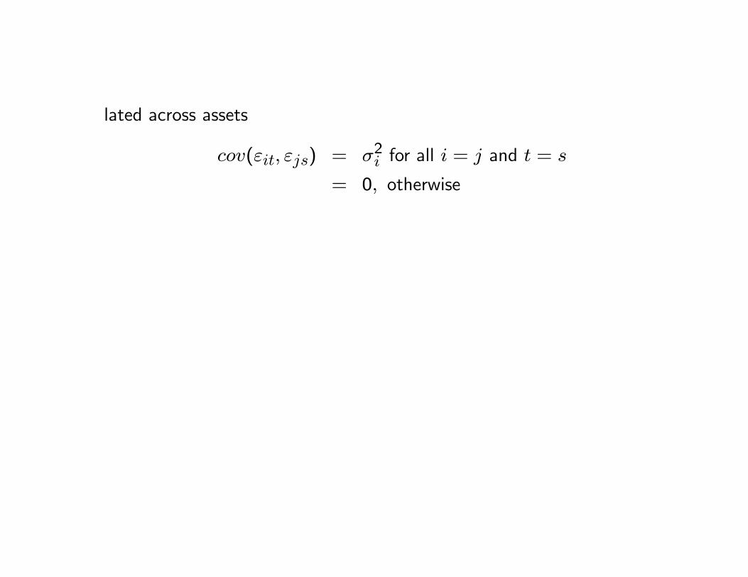
lated across assets

( ) = 2 for all = and =

= 0 otherwise

Remarks:

• Statistical modeling of returns involves statistical modeling of factors andresiduals

• Typical factor models have a small number of factors (e.g., 10)

• Multivariate modeling of factors is a relatively low dimensional problem

— Copula models are feasible for factors

— Multivariate GARCH (e.g. DCC) is feasible for factor covariances

• ( ) = 0 ( 6= ) ⇒ only need univariate statistical models for

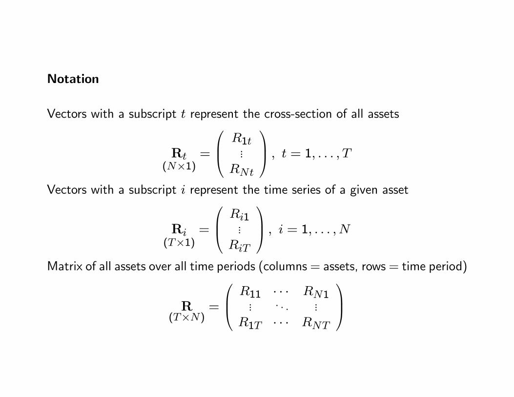
Notation

Vectors with a subscript represent the cross-section of all assets

R(×1)

=

⎛⎜⎝ 1...

⎞⎟⎠ = 1

Vectors with a subscript represent the time series of a given asset

R(×1)

=

⎛⎜⎝ 1...

⎞⎟⎠ = 1

Matrix of all assets over all time periods (columns = assets, rows = time period)

R(×)

=

⎛⎜⎝ 11 · · · 1... . . . ...

1 · · ·

⎞⎟⎠

Cross Section Regression

The multifactor model (1) may be rewritten as a cross-sectional regressionmodel at time by stacking the equations for each asset to give

R(×1)

= α(×1)

+ B(×)

f(×1)

+ ε(×1)

= 1 (2)

B(×)

=

⎡⎢⎣ β01...β0

⎤⎥⎦ =⎡⎢⎣ 11 · · · 1... . . . ...1 · · ·

⎤⎥⎦[εε

0|f] = D = (21

2)

Note: Cross-sectional heteroskedasticity

This representation is useful for risk analysis across assets.

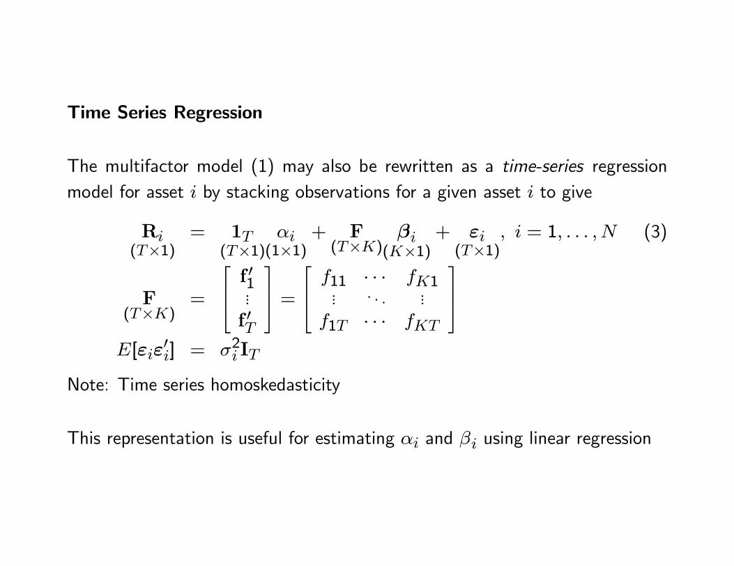
Time Series Regression

The multifactor model (1) may also be rewritten as a time-series regressionmodel for asset by stacking observations for a given asset to give

R(×1)

= 1(×1)

(1×1)

+ F(×)

β(×1)

+ ε(×1)

= 1 (3)

F(×)

=

⎡⎢⎣ f 01...f 0

⎤⎥⎦ =⎡⎢⎣ 11 · · · 1

... . . . ...1 · · ·

⎤⎥⎦[εε

0] = 2 I

Note: Time series homoskedasticity

This representation is useful for estimating and using linear regression

Multivariate Regression

Collecting data from = 1 allows the model (3) to be expressed as themultivariate regression

[R1 R ] = 1 [1 ] + F[β1 β ] + [ε1 ε ]

or

R(×)

= 1(×1)

α0(1×)

+ F(×)

B0(×)

+ E(×)

= XΓ0 + E

X(×(+1))

= [1... F] Γ0

((+1)×)=

"α0

B0

#

Alternatively, collecting data from = 1 allows the model (2) to beexpressed as the multivariate regression

[R1 R ] = [α α] +B[f1 f ] + [ε1 ε ]

or

R0(× )

= α(×1)

10(1× )

+ B(×)

F0(× )

+ E0(× )

= ΓX0 + E0

X0((+1)× )

=

"10F0

# Γ(×(+1))

= [α ... B]

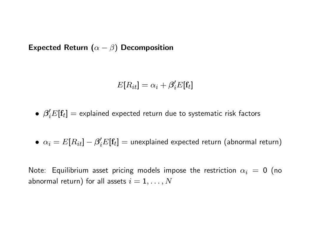
Expected Return (− ) Decomposition

[] = + β0[f]

• β0[f] = explained expected return due to systematic risk factors

• = []− β0[f] = unexplained expected return (abnormal return)

Note: Equilibrium asset pricing models impose the restriction = 0 (noabnormal return) for all assets = 1

Covariance Structure

Using the cross-section regression

R(×1)

= α(×1)

+ B(×)

f(×1)

+ ε(×1)

= 1

and the assumptions of the multifactor model, the ( ×) covariance matrixof asset returns has the form

(R) = Ω = BΩB0 +D (4)

Note, (4) implies that

() = β0Ωβ + 2() = β0Ωβ

() =β0Ωβh³

β0Ωβ + 2

´(β0Ωβ + 2)

i12

Conditional Covariance Structure

Let denote the information available at time We can allow the factorcovariances and residual variances to be time varying

f×1

= μ|−1 + ε

ε = Ω12 z⇒ (ε|−1) = Ω

× = ⇒ (|−1) = 2 = 1

Then the factor model conditional covariance matrix is

(R|−1) = Ω = BΩB0 +D

Note: We can also allow the factor betas to be time varying (i.e., B = B)

Portfolio Analysis

Let w = (1 ) be a vector of portfolio weights ( = fraction ofwealth in asset ). If R is the ( × 1) vector of simple returns then

= w0R =

X=1

Portfolio Factor Model

R = α+Bf + ε⇒ = w0α+w0Bf +w0ε = + β0f +

= w0α β0 = w0B = w0ε

() = β0Ωβ + () = w0BΩB

0w+w0Dw

Active and Static Portfolios

• Active portfolios have weights that change over time due to active assetallocation decisions

• Static portfolios have weights that are fixed over time (e.g. equally weightedportfolio)

• Factor models can be used to analyze the risk of both active and staticportfolios

Unconditional Asset Risk Measures: Factor Model and Normal Distrib-ution

= + β0f +

f ∼ (μ Ω) () = 2 ( ) = 0 for all

Then

[] = = + β0μ() = 2 = β0Ωβ + 2

=

rβ0Ωβ + 2

= + ×

= −

1

()

Note: In practice, = 0 is typically imposed so that = β0μ .

Conditional Asset Risk Measures: Factor Model and Normal Distribution

(|−1) = 2 = β0Ωβ + 2

=

rβ0Ωβ + 2

= + ×

= −

1

()

whereΩ is modeled as an EWMA or DCC and 2 is modeled as an EWMA

or GARCH.

Note 1: For daily data it is typically assumed that = 0

Note 2: We could also allow β = β (e.g. estimate β over rolling windowsfor each )

Factor Risk Budgeting

• Additively decompose (slice and dice) individual asset or portfolio returnrisk measures into factor contributions

• Allow portfolio manager to know sources of factor risk for allocation andhedging purposes

• Allow risk manager to evaluate portfolio from factor risk perspective

Factor Risk Decompositions

Assume asset or portfolio return can be explained by a factor model

= + β0f +

f ∼ (μ Ω) ∼ (0 2) ( ) = 0 for all

Re-write the factor model as

= + β0f + = + β0f + ×

= + β0f

β = (β0 )0 f = (f )0 =

∼ (0 1)

Then

2 = β0Ωβ Ω

=

ÃΩ 00 1

!

Linearly Homogenous Risk Functions

Let(β) denote the risk measures and as functions

of β

Result 1: (β) is a linearly homogenous function of β for =

and That is, (·β) =·(β) for any constant ≥ 0

Example: Consider (β) = (β) Then

( · β) =³ · β0Ω

· β

´12= ·

³β0Ωβ´12

= · (β)

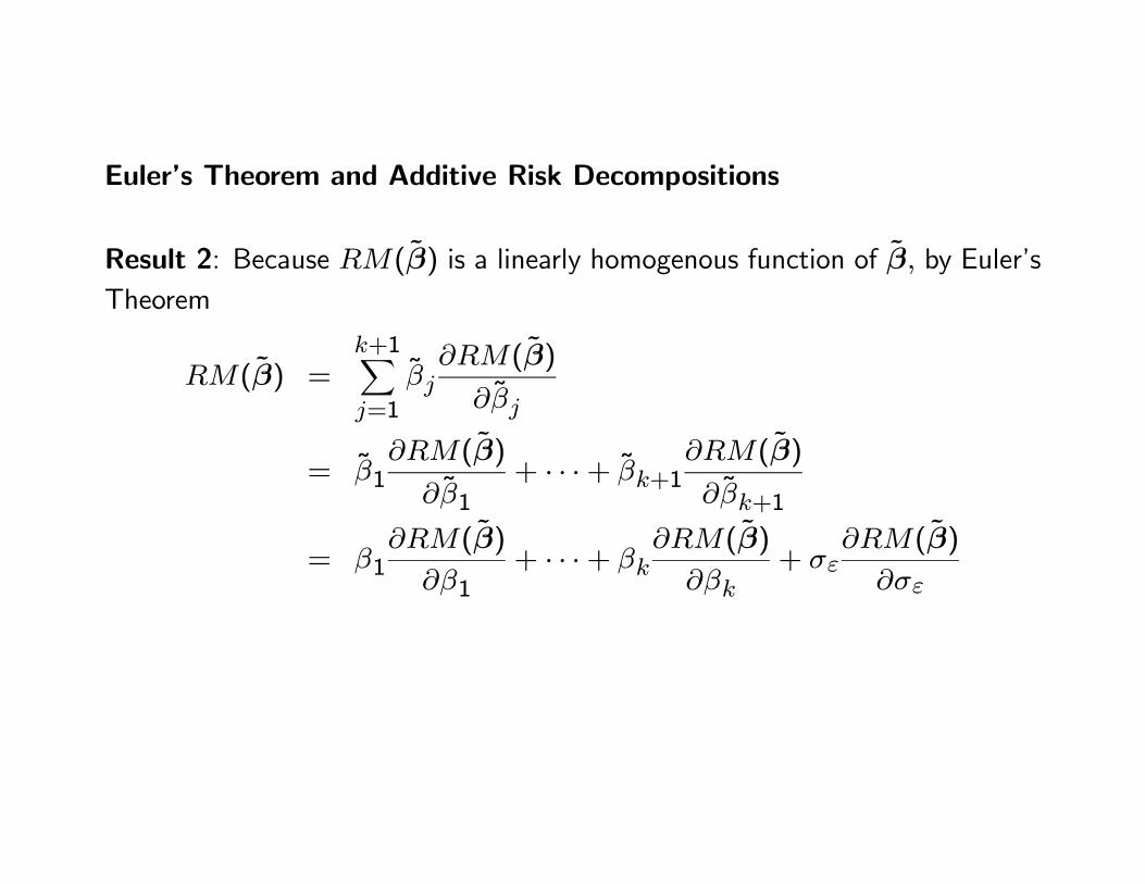
Euler’s Theorem and Additive Risk Decompositions

Result 2: Because (β) is a linearly homogenous function of β by Euler’sTheorem

(β) =+1X=1

(β)

= 1(β)

1+ · · ·+ +1

(β)

+1

= 1(β)

1+ · · ·+

(β)

+

(β)

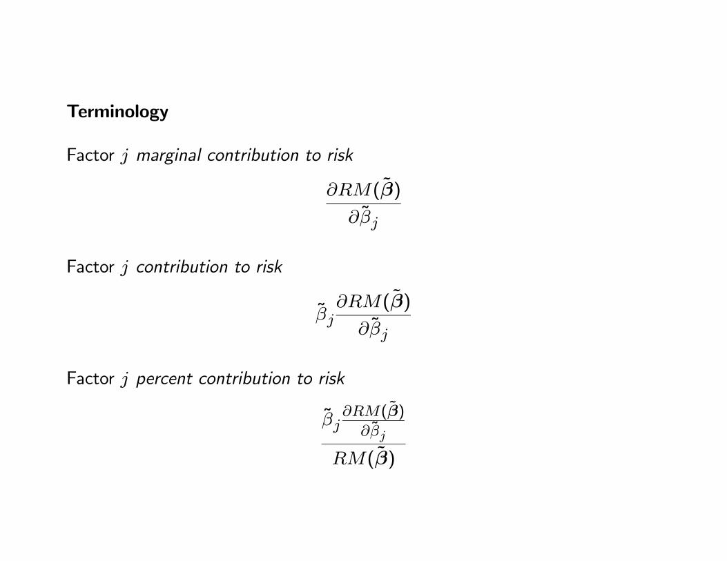
Terminology

Factor marginal contribution to risk

(β)

Factor contribution to risk

(β)

Factor percent contribution to risk

(β)

(β)

Analytic Results for (β) = (β)

(β) =³β0Ωβ´12

(β)

β=

1

(β)Ωβ

Factor = 1 percent contribution to (β)

1(1 ) + · · ·+ 2() + · · ·+ ( )

2(β)

Asset specific factor contribution to risk

2

2(β) = + 1

Results for (β) = (β) (β)

Based on arguments in Scaillet (2002), Meucci (2007) showed that

(β)

= [| =

(β)] = 1 + 1

(β)

= [| ≤

(β)] = 1 + 1

Remarks

• Intuitive interpretation as stress loss scenario

• Analytic results are available under normality

Marginal Contributions to Tail Risk: Non-Parametric Estimates

Assume and f are iid but make no distributional assumptions:

(1 f1) ( f ) = observed iid sample

Estimate marginal contributions to risk using historical simulation

[| = ] =

1

X=1

· 1½ d

− ≤ ≤ d +

¾

[| ≤ ] =1

[]

X=1

· 1½ d

≤

¾Problem: Not reliable with small samples or with unequal histories for

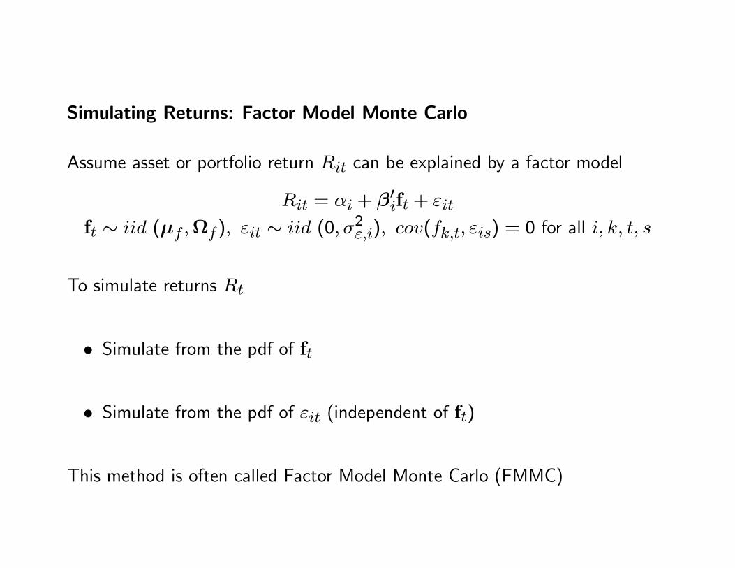
Simulating Returns: Factor Model Monte Carlo

Assume asset or portfolio return can be explained by a factor model

= + β0f +

f ∼ (μ Ω) ∼ (0 2) ( ) = 0 for all

To simulate returns

• Simulate from the pdf of f

• Simulate from the pdf of (independent of f)

This method is often called Factor Model Monte Carlo (FMMC)

Advantages of FMMC

• Number of factors is typically much smaller than the number of assets (e.g.5 factors vs. 1000 assets)

• Multivariate modeling of is feasible with a small number of factors

• Univariate models can be used for residuals because of independenceacross assets

• Dependence structure across assets is defined by factor loadings and de-pendence structure of factors

• Can deal with unequal histories for asset returns (e.g. hedge fund data)

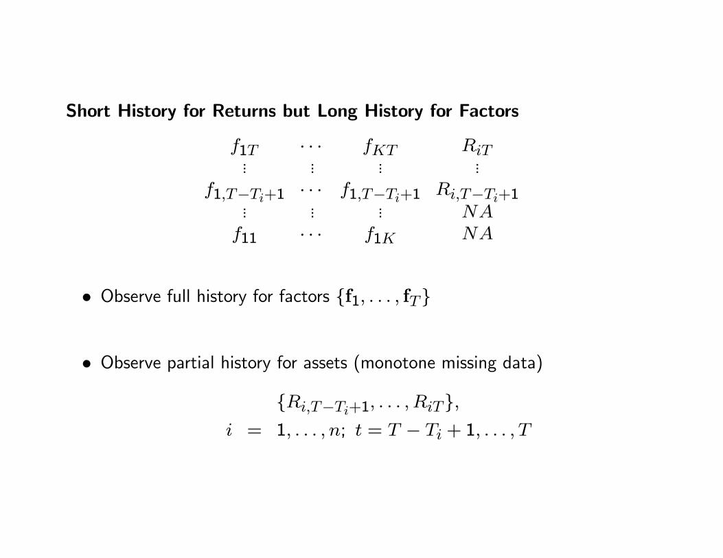
Short History for Returns but Long History for Factors

1 · · · ... ... ... ...1−+1 · · · 1−+1 −+1... ... ...

11 · · · 1

• Observe full history for factors f1 f

• Observe partial history for assets (monotone missing data)

−+1 = 1 ; = − + 1

Simulation Algorithm

• Estimate factor models for each asset using partial history for assets andrisk factors

= + β0f + = − + 1

• Simulate values of the risk factors from the pdf of f:

f∗1 f∗

• Simulate values of the factor model residuals from the pdf of

∗1 ∗

• Create pseudo factor model returns from fitted factor model parameters,simulated factor variables and simulated residuals:

∗1 ∗∗ = β

0f∗ + ∗ = 1

Simulating Factor Realizations: Distribution choices

• Multivariate distributions (e.g., multivariate normal, t, copula distributionsetc) (parametric, unconditional)

• Conditional multivariate distributions (e.g. normal DCC model)

• Empirical distribution (non-parametric, unconditional)

— Resample with replacement from observed history of factors

• Filtered historical simulation (semi-parametric, conditional)

— use local time-varying factor covariance matrices to standardize factorsprior to re-sampling and then re-transform with covariance matricesafter re-sampling

Simulating Residuals: Distribution choices

• Normal distribution (parametric, unconditional)

• Non-normal: Student’s t, Skewed Student’s t etc. (parametric, uncondi-tional)

• Empirical (resample with replacement from observed residuals) (nonpara-metric, unconditional)

• GARCH(1,1) (parametric, conditional)

• Filtered historical simulation (semi-parametric, conditional)

References

[1] Goldberg, L.R., Yayes, M.Y., Menchero, J., and Mitra, I. (2009). “ExtremeRisk Analysis,” MSCI Barra Research.

[2] Goldberg, L.R., Yayes, M.Y., Menchero, J., and Mitra, I. (2009). “ExtremeRisk Management,” MSCI Barra Research.

[3] Goodworth, T. and C. Jones (2007). “Factor-based, Non-parametric RiskMeasurement Framework for Hedge Funds and Fund-of-Funds,” The Euro-pean Journal of Finance.

[4] Jiang, Y. (200). Overcoming Data Challenges in Fund-of-Funds PortfolioManagement. PhD Thesis, Department of Statistics, University of Wash-ington.

[5] Meucci, A. (2007). “Risk Contributions from Generic User-Defined Fac-tors”, Risk.