Am I Getting a Good Deal? Reference-Dependent Decision Making when the Reference

Price is Uncertain

Jayson L. Lusk, Vincenzina Caputo, and Rodolfo M. Nayga, Jr.*

Abstract: Models of consumer decision making commonly incorporate reference-dependent

preferences. In these models, the reference point is typically assumed to be known to the

consumer. However, research on price recall and the reference formation process reveals that for

most consumers the reference price is often uncertain at the time of purchase. Reference price

uncertainty, which arises from price variability, creates ambiguity for the consumer about

whether they are getting a good or bad deal. This paper develops a model of consumer choice in

the presence of reference-dependent preferences when the reference price is uncertain. Data

from three separate studies that vary the product category, use of brand names, and the way

reference prices and reference price uncertainty are measured show that the new model generally

better describes consumer choice than conventional discrete choice models that either ignore

reference prices or treat reference prices as certain. Incorporating reference price uncertainty

tends to yield own-price elasticities that are more elastic (sometimes twice as elastic) than those

from more conventional reference-dependent models that treat the reference price as certain.

The new model provides insights into the effect of reducing reference price uncertainty on

consumer choice.

Keywords: reference-dependent preferences; reference price uncertainty; consumer demand;

discrete choice models

JEL codes: D03, D11, C25, Q11

Contact: Jayson Lusk, 411 Ag Hall, Oklahoma State University; Stillwater, OK, 74074;

jayson.lusk@okstate.edu; (405) 744-7465.

*Authors are Regents Professor and Willard Sparks Endowed Chair, Oklahoma State University;

Assistant Professor, Korea University; and Professor and Tyson Endowed Chair, University of

Arkansas and adjunct professor, Korea University and Norwegian Agricultural Economics

Research Institute.

1

Introduction

Motivated in part by the work of Kahneman and Tversky (1979) and Tversy and Kahneman

(1991), models of reference-dependent preferences have become ubiquitous in the study of

consumer choice. Nowhere is this more true than in the analysis of reference-prices and their

influence on shopping behavior (Briesch et al., 1997; Kalyanaram and Winer 1995; Mazumdar,

Raj, and Sinha, 2005; Neumann and Böckenholt, 2014; Winer 1995). Recent empirical

applications have incorporated reference price effects into models that explain travel choice

(Rose and Masiero, 2010), automobile demand (Mabit and Fosgerau, 2011), selection of travel

destination (Nicolau, 2011), environmental valuations (Hasund et al., 2011), and food choice (Hu

et al., 2006), among others. This literature captures the idea that consumers are loss-averse with

regard to price changes; prices above a reference price signal a “bad deal” (Weaver and

Frederick, 2012), and as such, price sensitivity is more pronounced above a reference price than

below.

Despite the widespread acceptance of reference-dependent models in economics,

psychology, and marketing, typical approaches tend to omit a potentially important behavioral

insight. Consumers are unlikely to know their reference prices with certainty. Introspectively,

many shoppers can attest to having faced uncertainty over whether they are “getting a good

deal”. How does reference price uncertainty affect choice, and what is the consequence of

ignoring this phenomenon when predicting consumer behavior? This paper addresses these

questions by developing and empirically estimating a model of consumer choice in the presence

of reference-dependent preferences when the reference price is uncertain.

That reference-price uncertainty has been largely overlooked is curious given several

strains of literature suggesting that this feature of the decision-making process is likely to be the

2

rule rather than the exception. First, it has commonly been assumed that reference-dependence is

a result of memory-based reference prices or a result of internal reference prices measured as a

function of prices previously paid (Briesch et al. 1997; Mazumdar, Raj, and Sinha, 2005).

However, there is ample evidence suggesting that consumers are unaware of past prices paid for

products – even products they just placed in their grocery cart (Dickson and Sawyer 1990;

Estelami and Lehmann, 2001; Urbany and Dickson 1991; Vanhuele and Drèze 2002; Moon et al.

2006). Studies typically find that less than 50% of shoppers can recall the exact prices paid for

products (Jensen and Grunert, 2014). If prices previously paid are not known with any degree of

accuracy, it is unlikely that reference-prices are known with certainty. Second, the growing

research on the reference-point formation process (e.g., Abeler et al., 2011; Baucells, Weber, and

Welfens, 2011; Ericson, and Fuster, 2011; Kőszegi and Rabin, 2006) highlights the fluidity of

the reference points and emphasizes the role of expectations in determining the reference price.

Given that expectations implicitly imply underlying stochasicity, it follows that reference-points

are unlikely deterministic. Finally, even in models which implicitly assume that reference prices

are known by the consumer, researchers typically use household scanner data to estimate each

consumer’s reference price (e.g., Briesch et al., 1997; Erdem, Mayhew, and Sun, 2001; Bruno,

Che, and Dutta, 2012). The econometrically-estimated reference prices are thus projected with

some level of uncertainty, which is typically ignored by analysts when fitting subsequent choice

models.

Our inquiry bears some similarity with many strains of related literature. For example,

some research has suggested that consumers have thresholds of price acceptance, and thus appear

to utilize something like reference-price bounds, rather than a single reference price (e.g., Han,

Gupta, and Lehmann, 2002; Terui and Dahana, 2006). Ghoshal et al. (2014) argued that

3

consumers encounter communications and brands sequentially, and a variety of prior experiences

serve to create multiple reference points. There is also a rich body of research on the extent to

which consumers undertake search costs to better form expectations to improve subsequent

choice (e.g., De los Santos, Hortacsu and Wildenbeest, 2012; Kim, Albuquerque, and

Bronnenberg, 2010; Mehta, Rajiv, Srinivasan, 2003), findings which relate to the argument that

reference price uncertainty arises from a lack of price knowledge. Related to search costs is the

concept of option-values or “commitment costs”, which arise when consumers have the ability to

delay a purchase and are uncertain about their ability to acquire information about the good in

the future (Zhao and Kling, 2004). As discussed in the reviews of Briesch et al. (1997) and

Mazumdar, Raj, and Sinha (2005), there are a number of studies analyzing whether reference

price(s) are internal (e.g., based on expectations or memories of prices previously paid) or

external (e.g. based on external notions of fairness or willingness-to-pay). The model developed

in this paper bears some superficial similarity to the general conceptual model derived by

Kőszegi and Rabin (2006), who consider a model with uncertainty in prices, where the reference

point is stochastic and endogenously determined.

Previous research, thus, recognizes the fact that consumers face price variability (as

indicated by the search cost literature), may have multiple reference points (as indicated by the

literature on price acceptance thresholds), and may interpret price changes or variability as

quality signals which may also affect reference points (Hardie, Johnson, and Fader, 1993). It is

not likely that any single model will unify all these strands of literature in a way that well

describes all contexts, nor is it likely that all the previously discussed issues are separately

identifiable (i.e., if there is absolutely no price variability, there is no need to search, and it is

unlikely that internal reference prices would exist). To the extent that past prices inform current

4

reference points, it seems reasonable to believe that previous (or currently expected) price

variability is intrinsically linked to reference-price variability (or what we call reference price

uncertainty).

The particular situation we aim to model is akin to shopping for a grocery item in a

particular store. In such cases, prices for each brand at a given retailer (and at the time of choice)

are known with certainty. Because the costs of the individual items are typically small relative to

income, consumers are unlikely to (at least at the time of item choice) engage in price search

across retailers. Thus, there is no uncertainty in the prices being charged for each item at the

given retailer (i.e., the prices are within eyesight), and at least for known brands, it is unlikely the

case that there is much of a price-quality correlation (and in our empirical analysis, prices are

uncorrelated with brands). However, there might be uncertainty about prices paid in the past or

charged by other retailers. In this context, most prior research has utilized consumers’ expected

price (or the price previously paid for the item) before they walked in the door to the retailer as

the reference point. Our model expands on this idea and considers not only what price a

consumer expects to be charged for an item but also about the expected variability of prices they

would expect to be charged across retailers. Just as much of previous work has used the mean

price expectation as the reference point, we use people’s stated level of expected price variability

in their market as the measure of reference price uncertainty.

The next section of the paper presents the model of reference-dependent preferences in

the presence of reference-price uncertainty. The following section discusses a few issues related

to the econometric estimation as a way of transitioning to the empirical analysis. The following

three sections present three separate empirical studies where the new model is implemented and

compared to conventional models that either ignore reference prices or assume reference-price

5

certainty. Three separate studies are conducted to determine the generalizability of our findings

and to determine how robust the results are with regard to: (i) variation in the product category,

(ii) use of brand names, and (iii) the way reference prices and reference price uncertainty are

measured.

All three studies are based on choice-experiments (Louviere, Hensher, and Swait, 2000)

conducted among random samples of the U.S. population. We test our model in three different

studies in three different product categories given that purchase frequencies and price knowledge

likely varies across product categories. Study 1 involves choices between four infrequently-

bought branded products (ketchup), where the mean and standard deviation of reference prices

are elicited by asking respondents to state prices associated with 90% confidence intervals.

Study 2 involves choices between frequently-bought fresh milk options that vary in fat content.

The final study investigates choices between six un-branded fresh meat items and two un-

branded, non-meat items selected from a grocery store for a meal; reference prices are elicited

for each product as is the uncertainty in each reference-price on a simple slider scale.

Adamowicz and Swait (2012) report the wide variation in repeat same-brand purchases for the

products utilized in this study; 55% of consumers’ milk purchases are of the same previously

purchased brand whereas the only 22% of ketchup purchases meet this criterion. Most fresh beef

and pork sold in grocery stores is unbranded. This variation in product category familiarity

provides variation in reference price uncertainty to test the robustness of the model. The final

section summarizes the findings and concludes with thoughts for future research.

Conceptual Model

6

Assume that individual i evaluates the desirability of a purchase option based on the product’s

price, 𝑝𝑗, relative to some internal, subjective price reference point, 𝑟𝑖𝑗, for the product.

Consumers perceive prices above the reference point (losses) differently than changes below the

reference point (gains), such that an individual’s utility from purchasing option j is:

(1) 𝑈𝑖𝑗 = 𝑉𝑖𝑗 + 휀𝑖𝑗 = 𝛼𝑗(𝑝𝑗 − �̃�𝑖𝑗)𝐼𝑟𝑖𝑗<𝑝𝑗 + 𝛽𝑗(𝑝𝑗 − �̃�𝑖𝑗)𝐼𝑟𝑖𝑗>𝑝𝑗 + 𝜏𝑗 + 휀𝑖𝑗

where 𝐼𝑟𝑖𝑗<𝑝𝑗 is an indicator variable taking the value of one when prices are higher than the

reference point (losses), 𝐼𝑟𝑖𝑗>𝑝𝑗is an indicator variable taking the value of one when prices are

lower than the reference point (gains), and 𝛼𝑗 and 𝛽𝑗 are price-sensitivity parameters, where it is

assumed that 𝛼𝑗 < 𝛽𝑗, implying that consumers are loss averse. The parameter 𝜏𝑗 represents an

alternative-specific constant indicating the utility of option j that is unexplained by price

variation, and 휀𝑖𝑗 reflects an idiosyncratic effect unobserved to the analyst.

Variations on the specification in (1) above have been explored in detail in previous

demand studies, and there is ample evidence to suggest support for the reference-price model,

i.e., that 𝛼 ≠ 𝛽 (Mazumdar, Raj, and Sinha, 2005). The key departure we take from these

previous studies is the intuitive assumption that individuals are uncertain about the reference

price and that, from the perspective of the individual, 𝑟𝑖𝑗 is a subjective random variable, as

denoted by �̃�𝑖𝑗 in equation (1). �̃�𝑖𝑗 is assumed to be distributed according to the probability

density function, 𝑓𝑖(𝑟𝑖𝑗) and the cumulative distribution function 𝐹𝑖(𝑟𝑖𝑗).

They key question is how individuals evaluate the desirability of a choice option when

the reference price is uncertain (i.e., when consumers are unsure of whether they are getting a

“good deal”). One approach is to assume consumers are risk neutral and that they evaluate the

7

desirability of an option based on the expected utility of the option, as given by the following

(the i subscript has been dropped for notational convenience):

(2) 𝐸[𝑉𝑗] = ∫ 𝛼𝑗(𝑝𝑗 − 𝑟𝑗)𝑝

−∞𝑓(𝑟𝑗)𝑑𝑟𝑗 + ∫ 𝛽𝑗(𝑝𝑗 − 𝑟𝑗)

∞

𝑝𝑓(𝑟𝑗)𝑑𝑟𝑗 + 𝜏𝑗.

The first integral is taken over all potential reference points less than the product price, in which

case the shopper experiences a loss and evaluates price changes according to the parameter 𝛼𝑗.

The second integral is taken over all potential reference points greater than the product price, in

which case the shopper experiences a gain and evaluates price changes according to the

parameter 𝛽𝑗. Expanding equation (2) yields:

(3) 𝐸[𝑉𝑗] = 𝛼𝑗𝑝𝑗 ∫ 𝑓(𝑟𝑗)𝑑𝑟𝑗𝑝

−∞− 𝛼𝑗 ∫ 𝑟𝑗𝑓(𝑟𝑗)𝑑𝑟𝑗

𝑝

−∞+ 𝛽𝑗𝑝𝑗 ∫ 𝑓(𝑟𝑗)𝑑𝑟𝑗

∞

𝑝− 𝛽𝑗 ∫ 𝑟𝑗𝑓(𝑟𝑗)𝑑𝑟𝑗

∞

𝑝+

𝜏𝑗

Note that ∫ 𝑓(𝑟𝑗)𝑑𝑟𝑗 = 𝐹(𝑝𝑗)𝑝

−∞ is the probability that the reference point is less than the

observed price and that ∫ 𝑓(𝑟𝑗)𝑑𝑟𝑗 = 1 − 𝐹(𝑝𝑗)∞

𝑝 is the probability that the reference point is

greater than the observed price. If the subjective reference price distribution is Normally

distributed then, 𝐹(𝑝𝑗) = 𝛷((𝑝𝑗 − �̅�𝑗)/𝜎𝑗) where �̅�𝑗 is the mean subjective reference price (from

the particular consumer’s perspective), 𝜎𝑗 is the standard deviation of the subjective reference

price (again, from the consumer’s perspective), and 𝛷 is the standard Normal cdf. Substituting,

we how have:

(4) 𝐸[𝑉𝑗] = 𝛼𝑗𝑝𝑗𝐹(𝑝𝑗) − 𝛼𝑗 ∫ 𝑟𝑗𝑓(𝑟𝑗)𝑑𝑟𝑗𝑝

−∞+ 𝛽𝑗𝑝𝑗(1 − 𝐹(𝑝𝑗)) − 𝛽𝑗 ∫ 𝑟𝑗𝑓(𝑟𝑗)𝑑𝑟𝑗

∞

𝑝+ 𝜏𝑗.

The expression ∫ 𝑟𝑗𝑓(𝑟𝑗)𝑑𝑟𝑗𝑝

−∞ is the mean of the truncated distribution for r (truncated

from above at p) multiplied by the probability of r being less than p. That is, ∫ 𝑟𝑗𝑓(𝑟𝑗)𝑑𝑟𝑗𝑝

−∞=

𝐸[𝑟𝑗|𝑟𝑗 < 𝑝𝑗]𝐹(𝑟𝑗). For a Normal distribution, 𝐸[𝑟𝑗|𝑟𝑗 < 𝑝𝑗] = �̅�𝑗 − 𝜎𝑗[𝜙(𝜃)/𝛷(𝜃)], where

8

𝜃 = (𝑝𝑗 − 𝑟�̅�)/𝜎𝑗, and where 𝜙 is the standard normal pdf. For the case where truncation is from

below (i.e., when the reference price exceeds observed price), then ∫ 𝑟𝑗𝑓(𝑟𝑗)𝑑𝑟𝑗∞

𝑝=

𝐸[𝑟𝑗|𝑟𝑗 > 𝑝𝑗](1 − 𝐹(𝑟𝑗)) and for a Normal distribution, 𝐸[𝑟𝑗|𝑟𝑗 > 𝑝𝑗] = �̅�𝑗 + 𝜎𝑗[𝜙(𝜃)/(1 −

𝛷(𝜃))]. Plugging these values into equation (4), and assuming the perceived reference price is

normally distributed, yields:

(5) 𝐸[𝑉𝑗] = 𝛼𝑗𝑝𝑗𝛷(𝜃) − 𝛼𝑗𝛷(𝜃){�̅�𝑗 − 𝜎𝑗 [𝜙(𝜃)

𝛷(𝜃)]} + 𝛽𝑗𝑝𝑗(1 − 𝛷(𝜃)) − 𝛽𝑗(1 − 𝛷(𝜃)){�̅�𝑗 +

𝜎𝑗 [𝜙(𝜃)

1−𝛷(𝜃)]} + 𝜏𝑗.

Slightly simplifying, equation (5) can be written as:

(6) 𝐸[𝑉𝑗] = 𝛼𝑗𝛷(𝜃) {𝑝𝑗 − �̅�𝑗 + 𝜎𝑗 [𝜙(𝜃)

𝛷(𝜃)]} + 𝛽𝑗(1 − 𝛷(𝜃)){𝑝𝑗 − �̅�𝑗 − 𝜎𝑗 [

𝜙(𝜃)

1−𝛷(𝜃)]} + 𝜏𝑗.

Equation (6) has an intuitive interpretation. To see this, (6) can be described in general

terms as:

(7) 𝐸[𝑉𝑗] = 𝛼𝑗𝑃𝑟𝑜𝑏[𝑟𝑗 < 𝑝𝑗]{𝑝𝑗 − 𝐸[𝑟𝑗|𝑟𝑗 < 𝑝𝑗]} + 𝛽𝑗𝑃𝑟𝑜𝑏[𝑟𝑗 > 𝑝𝑗]{{𝑝𝑗 − 𝐸[𝑟𝑗|𝑟𝑗 > 𝑝𝑗]} +

𝜏𝑗.

For the first part of the expression, the “loss averse” price parameter, 𝛼𝑗, is multiplied by the

probability that the observed price exceeds the reference point, 𝑃𝑟𝑜𝑏[𝑟𝑗 < 𝑝𝑗], which in turn is

multiplied by the difference between the price of the option, 𝑝𝑗, and the expected reference price

given that observed price is greater than the reference price (the mean of the reference price

truncated from below at the observed price), 𝐸[𝑟𝑗|𝑟𝑗 < 𝑝𝑗]. The second part of the expression

analogously multiplies the “gain” price parameter, 𝛽𝑗, by the difference in the observed price and

expected reference point, conditional on the reference point being greater than the price. In this

9

way, (6) and (7) can be seen as a probabilistic expression of the original formulation stated in

(1).

Empirical Model and Estimation

Equation (6) forms the basis for estimation for Studies 1 and 2. In particular, equation (6) is

substituted into the following random utility model

(7) 𝑈𝑖𝑗 = 𝐸[𝑉𝑖𝑗] + 𝑒𝑖𝑗 + 휀𝑖𝑗.

Assuming 휀𝑖𝑗 are distributed iid type I extreme value, the multinomial logit specification results:

(8) Prob j is chosen by i = 𝑒𝐸[𝑉𝑖𝑗]+𝑒𝑖𝑗

∑ 𝑒𝐸[𝑉𝑖𝑘]+𝑒𝑖𝑘𝐽𝑘=1

.

The term 𝑒𝑖𝑗 reflects a mean-zero, Normally distributed alternative-specific effect.

This specification is a mixed-logit, error-components model. Scarpa, Ferrini, and Willis

(2005) suggest a version of this specification, where 𝑒𝑖𝑗 is the same for all alternatives except the

status-quo (or “no purchase”) option, for which there is no error component. This approach

reflects a parsimonious way to accommodate differential substitution patterns among the status-

quo (or “no purchase”) alternative and the other alternatives in the choice set. We specify our

model such that error-component is assumed to be individual-specific to account for the repeated

nature of the choice data. Moreover, the specification reflects the panel nature of our data and

captures some degree of respondent heterogeneity. The utility of the “no purchase” option is

normalized to zero for identification purposes. The likelihood function defined by the

probability statement in (8) does not have a closed form due to the presence of the random term

𝑒𝑖𝑗. We integrate this term out of the likelihood function using Gaussian quadrature.

To judge the suitability of the new model specification in (6), we estimate four models

that are increasing in complexity. The four models estimated are:

10

Model 1: A standard approach that has single linear price effect that assumes no

reference-dependence (i.e., it is assumed that 𝑉𝑖𝑗 = (𝛼 = 𝛽)𝑝𝑗 + 𝜏𝑗).

Model 2: A model with alternative-specific linear price effects that assumes no reference-

dependence (i.e., it is assumed that 𝑉𝑖𝑗 = (𝛼𝑗 = 𝛽𝑗)𝑝𝑗 + 𝜏𝑗).

Model 3: A reference-dependent model where reference price is assumed known with

certainty (i.e., it is assumed that 𝑉𝑖𝑗 = 𝛼𝑗(𝑝𝑗 − �̅�𝑖𝑗)𝐼�̅�𝑖𝑗<𝑝𝑗 + 𝛽𝑗(𝑝𝑗 − �̅�𝑖𝑗)𝐼�̅�𝑖𝑗>𝑝𝑗 + 𝜏𝑗).

Model 4: A reference-dependent model with reference price uncertainty (i.e., it is

assumed that 𝑉𝑖𝑗 is defined as in equation (6)).

Models are compared based on the percentage of choices correctly predicted and the AIC

and BIC model selection criteria. Model 1 is a nested version of Model 2, and as such likelihood

ratio tests can be used to test the null that price effects are not alternative specific. Models 3 and

4 do not nest models 1 or 2 via parametric restrictions because of the introduction of the variable

�̅�𝑖𝑗, which is subtracted from 𝑝𝑗.

Study 1

The first study investigates consumer demand for a relatively infrequently bought item, ketchup,

for which there are well known brand names. Given that ketchup is not bought at a high

frequency (only 11% of our sample report buying ketchup at least once a week) and there are

relatively few repeat-brand purchases, we expected that price may not be as important a factor

driving choice as is the case for other products and reference-prices are likely to be relatively

uncertain.

Methods and Procedures

11

Study 1 utilizes data from 216 subjects, each of whom made 25 choices (for a total of 5,400

choices) between four ketchup brands (i.e., Hunt’s, Heinz, Del Monte, and Red Gold). Each

choice task also included a fifth “no purchase” option that indicated, “if options A, B, C, and D

were all that were available I would not buy ketchup from this store. In each question, the

options were offered at one of five levels ($1.50, $2.25, $3.00, $3.75, and $4.50) chosen to

encompass the range of ketchup prices in major retailer supermarket outlets. Out of the 54=625

different choice questions possible, we selected 25 that comprised an orthogonal fractional

factorial design in which the price of each brand is uncorrelated with all other brands. The choice

questions were randomly ordered across respondents. Data were collected from responses to an

online questionnaire showing images of the ketchup bottles with the respective brands and

prices. Participants were recruited by the online survey software provider Qualtrics and their

associated partners.

After answering the choice questions, respondents’ reference prices were elicited by

asking, “What price would you expect a grocery store to charge for your favorite brand of a 36

ounce (oz) bottle of tomato ketchup?” This approach to eliciting the reference price presumes

that expectations are the appropriate reference point (Ericson, and Fuster, 2011; Kőszegi and

Rabin, 2006) and that the most recently purchased brand’s price is the likely reference (Briesch

et al., 1997). Moreover, in study 1 we only asked about one reference price, and assume it is the

same for all brands – an assumption generally supported by the empirical work of Briesch et al.

(1997). Responses to this question are used to specify the mean price reference point, �̅�𝑖.

To elicit uncertainty in the reference price, respondents were asked to respond to the

following: “In 90% of stores I would expect to find the price of my favorite brand of a 36 ounce

(oz) bottle of tomato ketchup to be no higher than . . .”. Another similar question was asked

12

except that “higher than” was replaced by “lower than”. To calculate reference price uncertainty

we utilize the answers to these two questions, denoted 𝑟𝑖,0.9 and 𝑟𝑖,0.1, to back out the value 𝜎𝑖

that appears in equation (6). In particular, note that familiar z-score implies that at the 90th

percentile 1.282 = (𝑟𝑖,0.9 − �̅�𝑖)/𝜎𝑖, such that 𝜎𝑖 = (𝑟𝑖,0.9 − �̅�𝑖)/1.282. An analogous value can

be derived using the price stated for the 10th

percentile, and we take the mid-point of these two

estimates to define 𝜎𝑖 for each person.

Additional details on the survey questions, along with descriptive statistics are provided

in the appendix.

Estimation Results and Model Comparisons

Table 1 reports the estimates for each of the four models fit to the ketchup data. A likelihood

ratio test rejects model 1 in favor of model 2 (chi-square value of 37 with 3 degrees of freedom;

p-value<0.001), supporting the existence of alternative-specific price effects. All model fit

criteria favor model 3 over model 2, suggesting that the reference-dependent model outperforms

the specifications that ignore consumers’ internal reference prices. Model 4, which incorporates

reference price uncertainty, is the best fitting model. Although it contains the same number of

parameters as model 3, it has a higher percentage of correct predictions and lower AIC and BIC

values.

Discussion

Models 3 and 4 reveal the strong asymmetry that exists between price changes above and below

the reference point. For example, according to model 4, a $1 increase in price for brand 2

13

reduces utility by -2.184 if the price is above the reference point (a loss) but only reduces utility

by -0.482 if the price is below the reference point.

Although model 4 provides a better fit to the data, it is unclear what practical implications

are implied by the model, particularly because the model coefficients appear similar for models 3

and 4. To provide insight into this issue, Table 2 reports the own-price arc-elasticities implied by

each of the models. Because of the potential asymmetry in price effects implied by the

reference-price models, arc-elasticities are calculated for a price increase relative to the mid-

point of the prices used in the experimental design ($3) and for a price decrease relative to this

mid-point (note: the mean elicited reference price was $2.62 and the median was $2.5; the mean

implied standard deviation of the subjective reference price distribution was $0.46).

In the absence of the new Model 4 derived in this paper, Model 3 which assumes

reference-dependent preferences but ignores uncertainty in the reference price would be the

preferred specification. As such the comparison of elasticities across models 3 and 4 are most

germane. Model 4 implies substantially more price sensitivity to price increases and decreases

than does model 3. For example, for a price increase, the own-price elasticity of demand for

brand 2 is -1.337 for Model 3 but the same value is -2.468 for Model 4, 1.84 times more elastic.

Somewhat ironically, Model 4 yields own-price elasticities that are, at least for price increases,

more comparable to Models 1 and 2, which completely ignore reference-dependent preferences.

The last rows in table 2 show the effect of reducing the uncertainty in the reference price.

By definition, Models 1, 2, and 3 imply no change in probability of purchase because reference

price uncertainty does not enter into these models. To simulate the effect of such a change for

Model 4, each person’s implied reference price uncertainty,𝜎𝑖, was reduced by 25%, and the

probabilities of purchase were re-calculated. Table 2 expresses the change in market share in

14

elasticity terms. For example, a 1% reduction in 𝜎𝑖 for each person results in a 0.02% increase in

probability of purchasing brand 2 and a 0.025% reduction in the probability of purchasing brand

3. The effects of a change in reference price uncertainty on probabilities of purchase are small

relative to own-price changes.

Figure 1 also illustrates the practical implications of making inferences based on the

competing models by showing the implied demand curves for Heinz ketchup over the price

ranges utilized in the experimental design (holding prices of all other brands at their means). At

lower price levels (those less than the mean), Model 3 under-predicts market share relative to all

other models, which tend to yield similar market share estimates. At higher prices (higher than

the mean), the new reference price uncertainty model (model 4) yields smaller market shares

than the other models. Over the range of prices likely to be most relevant (say from $2.50 to

$3.50), demand is much more elastic for model 4 than for the other models.

Study 2

The second study moves to a more frequently bought item, milk, for which brand names are less

ubiquitous in a given location and other quality factors – like fat content – are likely to be more

determinative. About 64% of respondents in our sample reported buying milk at least once a

week, and as such, we expected reference price uncertainty to be lower for this product category

than for ketchup.

Methods and Procedures

Study 2 utilizes data from 222 subjects, each of whom made 25 choices (for a total of 5,500

choices) between four fat-content differentiated conventional milk products commonly sold in

grocery stores (skim, 1% reduced fat, 2% reduced fat, and whole) listed at different prices. In

15

addition to these options, each choice task also included a fifth “no purchase” option. Prices of

each fat option varied among five levels ($1.50, $2.25, $3.00, $3.75, or $4.50) across choice

questions. As in study 1, an orthogonal fractional factorial design was generated to reduce the

54=625 possible choice sets to 25 in which the price of each milk option is uncorrelated with the

prices of the other three types of milk. Also, as in Study 1, the order of the choices was

randomly varied across respondents. Data were collected from responses to an online

questionnaire showing images of milk jugs with fat-content labels and prices. Participants were

recruited by the online survey software provider Qualtrics and their associated partners.

Reference prices and reference price uncertainties were elicited in an analogous way to that

described in Study 1. Additional details on the survey questions, along with descriptive statistics

are provided in the appendix.

Estimation Results and Model Comparisons

Table 3 reports the estimates for each of the four models fit to the milk data. A likelihood ratio

test rejects model 1 in favor of model 2 (chi-square value of 43 with 3 degrees of freedom; p-

value<0.001), supporting the existence of alternative-specific price effects. All model fit criteria

favor model 3 over model 2, suggesting that the reference-dependent model outperforms the

specifications that ignore the reference point. As was the case with study 1, Model 4, which

incorporates reference price uncertainty, is the best fitting model according to all three model fit

criteria.

Discussion

16

The estimates in table 3 again reveal a high degree of asymmetry between price changes above

and below the reference point. For example, for model 4 and option 1, the degree of price

sensitivity is 1.490/0.394 = 3.55 times higher for losses relative to “gains”. Table 4 further

illustrates the differences in practical implications implied by each model by reporting own-price

arc-elasticities for price increases and decreases relative to the mid-point of the prices used in the

experimental design ($3.50) (note: the mean elicited reference price was $3.11 and the median

was $3; the mean implied standard deviation of the subjective reference price distribution was

$0.42).

As was the case in study 1, Table 4 shows that for study 2, Model 4 implies substantially

more price sensitivity to price increases and decreases than does model 3. Most notably, for a

price decrease, the implied own-price elasticity of demand for option 1 was -1.753 for Model 3

but was -4.059 for Model 4. Again, Model 4, which includes reference prices and reference

price uncertainty, yields own-price elasticities that are more comparable to Models 1 and 2,

which completely ignore reference-dependent preferences. The last rows in table 4 show the

effect of reducing the uncertainty in the reference price, and again, the effects are relatively

small.

Figure 2 illustrates the demand for whole milk for the four competing models. As was

the case with study 1, the standard reference-dependent model (model 3), under-estimates market

share relative to the other models at lower price levels. By contrast, model 4 suggests lower

market share estimates than the other models at higher price levels. Over the mid-range of

prices, the new model 4 implies more elastic demand that the other models, particularly model 3.

Study 3

17

The third study departs from the first two in several important ways. First, rather than asking

about choices within a narrow product category, respondents were asked to make a main meal

choice among several meat and non-meat items in a grocery setting. Second, rather than

assuming a common reference price for all items, we elicit a reference price for each item.

Finally, because we hypothesized that it might be relatively difficult for respondents to state

reference prices and the 90th

and 10th

percentiles, the Study 3 utilized an easy-to-answer slider

scale of reference price uncertainty for each item.

Methods and Procedures

This study utilizes data from a choice-experiment conducted among 1,018 respondents, each of

whom made nine choices between six meat and two non-meat items bought in a grocery store for

dinner. Preceding the choice questions was the verbiage: “Imagine you are at the grocery store

buying the ingredients to prepare a meal for you or your household. For each of the following

nine questions that follow, please indicate which meal you would be most likely to buy.”

Each of the questions was identical except that the prices varied across each question.

Each question had nine pictured options (ground beef, steak, pork chop, ham, chicken breast,

chicken wing, rice and beans, pasta, and one “no purchase” option) and the price of each option

was varied at three levels. The prices appearing in each choice were determined by a main

effects orthogonal fractional factorial design. A perfectly orthogonal design (in which prices of

each choice alternative were uncorrelated with each other alternative) required 27 choices. The

27 choices were blocked into three sets of nine, and each person was randomly assigned to one

of the three blocks. The order in which the meal options appeared in the choice set was

randomly varied across subjects.

18

Reference prices for each product were measured by asking respondents about the

expected value of each product’s price in their area. They were asked, “What is your best

estimate of the average price that grocery stores, supermarkets, and wholesale stores charge for

the following products in your area?” Following this, respondents were asked, “On a scale from

0 to 100, where 0 indicates absolute uncertainty and 100 indicates absolute certainty, how

confident are you in your previous price estimate for the following products?” Respondents

indicated their answers using a slider scale that ranged between 0 and 100 in increments of one.

We asked the uncertainty question in this way because we hypothesized that this question is

easier for subjects to answer than asking them to state percentiles or standard deviations.

Participants were recruited by Survey Sampling International and completed an online

survey hosted on Qualtrics. Additional details on the survey questions, along with descriptive

statistics are provided in the appendix.

To incorporate the subjects’ stated level of reference-price uncertainty into our estimated

model, we specify the standard deviation in equation (6), as follows: 𝜎𝑖𝑗 = √𝛿𝑗exp (𝛾𝑗(100−𝑡𝑖𝑗)

100),

where 𝛿𝑗 is a parameter to be estimated corresponding to the standard deviation of the reference-

price distribution for good j, 𝑡𝑖𝑗 is individual i’s stated level of certainty in the reference price for

good j which is reverse coded (to convert certainty to uncertainty) and rescaled to range between

0 and 1, and where 𝛾𝑗 is a parameter to be estimated that translates individual-specific

uncertainty, as measured on the survey, to changes in the standard deviation of the subjective

reference-price distribution.

For sake of clarity, Model 4 estimated is estimated as:

19

(9) 𝐸[𝑉𝑗] = 𝛼𝑗𝛷(𝑝𝑗−�̅�𝑖𝑗

√𝛿𝑗 exp(𝛾𝑗100−𝑡𝑖𝑗

100)

)

{

𝑝𝑗 − �̅�𝑖𝑗 +√𝛿𝑗 exp (𝛾𝑗100−𝑡𝑖𝑗

100)

[ 𝜑

(

𝑝𝑗−�̅�𝑖𝑗

√𝛿𝑗 exp(𝛾𝑗

100−𝑡𝑖𝑗100 )

)

𝛷

(

𝑝𝑗−�̅�𝑖𝑗

√𝛿𝑗 exp(𝛾𝑗

100−𝑡𝑖𝑗100

))

]

}

+

𝛽𝑗 (1 − 𝛷(𝑝𝑗−�̅�𝑖𝑗

√𝛿𝑗 exp(𝛾𝑗100−𝑡𝑖𝑗

100)

))

{

𝑝𝑗 − �̅�𝑖𝑗 −√𝛿𝑗 exp (𝛾𝑗100−𝑡𝑖𝑗

100)

[ 𝜑

(

𝑝𝑗−�̅�𝑖𝑗

√𝛿𝑗exp (𝛾𝑗

100−𝑡𝑖𝑗100

))

1−𝛷

(

𝑝𝑗−�̅�𝑖𝑗

√𝛿𝑗exp (𝛾𝑗

100−𝑡𝑖𝑗100

))

]

}

+ 𝜏𝑗 .

The data consist of the experimentally-designed prices used in the choice experiment, 𝑝𝑗, and the

stated means and uncertainty in the reference price, �̅�𝑖𝑗 and 𝑡𝑖𝑗. The estimated parameters are 𝛼𝑗,

𝛽𝑗, 𝜏𝑗, 𝛿𝑗 and 𝛾𝑗.

Estimation Results and Model Comparisons

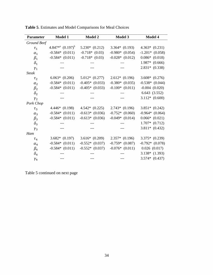
Table 5 reports the estimation results for Models 1-4. A likelihood ratio test favors Model 2 over

Model 1 (chi-square value of 135 with 7 degrees of freedom; p-value<0.001). Thus, the data

suggest alternative-specific price effects. For example, respondents are more sensitive to a

change in price for ground beef (-0.718) than they are for steak (-0.405). Qualitatively, Model 3

appears to be an improvement over Model 2 as the results are consistent with loss aversion (i.e.,

𝛼𝑗 < 𝛽𝑗) for every good, and the magnitude of the difference is pronounced. In fact, for a couple

of goods (e.g., chicken breast and pasta), 𝛽𝑗 is not significantly different from zero, meaning

people basically ignore price changes when they are below their reference point. Despite this,

the AIC and BIC are higher for Model 3 than for Models 1 and 2, meaning that the reference-

20

dependent model does not appear to fit the data as well as the more conventional specifications

according to these criteria.

The new specification, Model 4, has the best model fit according to percent of choices

correctly predicted; however, Model 4 has higher AIC and BIC values than Model 2. For Model

4, all the 𝛾𝑗 parameters are positive, as expected, meaning that higher stated reference price

uncertainty on the survey translated into a higher standard deviation around the reference price

distribution. The estimated 𝛿𝑗 parameters are all positive and most are significant, meaning that

there is indeed significant uncertainty in reference prices, which confirms the intuition and need

for this type of model.

One curious aspect associated with model 4 is that several of the 𝛽𝑗 parameters are

positive and statistically significant (although, they are qualitatively small). Taken literally, this

would mean that people prefer paying higher prices when prices are below their reference point.

Such a finding could be rationalized if people associate low prices (prices below reference

points) with signals of low quality. In study 1, quality was likely inferred from brand, and in

study 2, fat-content signaled a key quality attribute; however, in study 3, all products were

unbranded with regard to any quality information, raising the possibility that price was used to

infer quality (Bagwell and Riordan, 1991; Milgrom and Roberts, 1986; Zeithamal, 1988). This

result could also perhaps reflect disadvantageous inequality aversion as described by Fehr and

Schmidt (1999) (i.e., the buyer does not want to take advantage of a seller or to appear “cheap”).

Discussion

Table 6 reports own-price elasticities for the four model specifications. For price increases, we

observe a similar pattern of results as in Studies 1 and 2. Model 4 yields own-price elasticities

21

that are more elastic than those implied by Model 3 but that are more comparable to Models 1

and 2. However, for price decreases, the implied own-price elasticities were most inelastic for

Model 4. The final rows in table 6 report the effect of reducing reference price uncertainty for

each item (assuming all other item’s reference price uncertainty remains unchanged). For each

good, reducing the uncertainty around the product’s reference price increases the likelihood of

purchase. In general, a 1% reduction in the standard deviation of the reference price for a good

translates into a 0.04% to 0.07% increase in choice probability for that good.

Figure 3 illustrates the demand curve for ground beef (one of the most commonly chosen

items in the choice experiment) for the four competing models. Interestingly, models 3 and 4

never intersect, and the market share predictions of model 4 are always less than that for model

3. The bottom of table 5 shows that model 4 is superior to model 3 in terms of every fit critieria

considered. The predictions of model 4 closely mirror that for model 1 for higher price levels,

but for prices less than about $3, model 4 implies a near-linear price response whereas models 1

and 2 imply more elastic price responses.

Conclusions

While models incorporating reference dependent preferences are widely used, it is typically

assumed that the decision maker knows their reference points with certainty. In the case of

price-based reference points, this is a tenuous assumption given that there is ample evidence that

consumers are unaware of past prices paid for products, even for recently purchased products.

Consumers tend to poorly remember previously paid prices (which are often thought to form the

basis for reference points). This paper introduced a new conceptual model that incorporates

reference-price uncertainty into a random utility model of consumer choice and applied the

model to three different studies.

22

The first two studies showed that that the new model uniformly outperformed models that

either ignore reference prices or assumed reference prices were certain. In the third study, the

new model uniformly outperformed the model assuming reference-price certainty and

outperformed the models ignoring reference prices according to one out of three fit criteria.

Overall, the results from the three studies support the idea that reference-price uncertainty is an

important feature of consumer choice. They also suggest that the degree of reference price

uncertainty is linked to the nature of the products under evaluation (e.g., how frequently the

product is being purchased by consumers).

Results from the new model yield predictions that are often starkly at odds with

reference-price models that assume certainty in the reference price. In general, we tend to find

that incorporating reference price uncertainty results in more elastic own-price demand

elasticities than those implied by reference-price models which assume reference-price certainty.

In many cases, allowing for uncertainty more than doubles the size of the own-price elasticity.

We also tend to find, somewhat ironically, that elasticities implied from the new model are more

similar to models which ignore reference prices all together than they are to models that allow

reference prices but assume they are certain. This finding likely results because the new model,

while allowing for asymmetric price responses above and below a reference point, essentially

averages across this kink in the demand curve depending on the degree of reference price

uncertainty. This leads to an “effective” demand curve that is more continuous than the sharply

discontinuous demand curve implied by models that assume the reference price is known with

certainty.

This research highlights a number of issues that warrant future investigation. In

particular, contrasting study 3 with studies 1 and 2 suggests that the way in which reference

23

prices and reference-price uncertainty are measured in a survey may play a role in whether

reference-dependent models (with or without uncertainty) best describe choice; and at this point,

it is unclear which types of questions are likely to be most appropriate. Moving beyond survey-

based approaches to the analysis of scanner data, for example, presents challenges in how to

measure reference-price uncertainty. There is a large literature suggesting alternative models for

estimating reference prices from household scanner data. The typical approach relies on past-

prices previously paid by the consumer (Briesch et al., 1997; Mazumdar, Raj and Sinha, 2005),

but it is unclear whether reference-price uncertainty should be inferred from the distribution of

previously paid prices, the variance of the error term in the reference-price formation

econometric model, or some other metric like the standard deviation of prices currently being

paid by other consumers in the same geographic area.

Despite these challenges, developments in the literature on endogenous and expectation-

based reference point formation appear promising. This paper brought the idea of stochastic

reference points into a model of consumer choice, which also appears to have promise in

explaining phenomena of interest to a broad array of consumer and decision researchers.

24

References

Abeler, J., A. Falk, L. Goette, and D. Huffman. (2011). “Reference Points and Effort Provision.”

American Economic Review 101:470-492.

Adamowicz, W. L., and J.D. Swait. (2012). “Are Food Choices Really Habitual? Integrating

Habits, Variety-Seeking, and Compensatory Choice in a Utility-Maximizing

Framework.” American Journal of Agricultural Economics. 95:17-41.

Bagwell, K., and M.H. Riordan. (1991). “High and Declining Prices Signal Product Quality.”

American Economic Review 81:224-239.

Baucells, M., M. Weber, and F. Welfens. (2011). “Reference-Point Formation and Updating.”

Management Science 57(3):506-519.

Briesch, R.A., L. Krishnamurthi, R. Mazumdar, and S.P. Raj. (1997). “A Comparative Analysis

of Reference Price Models.” Journal of Consumer Research 24:202-214.

Bruno, H.A., H. Che, and S. Dutta. (2012). “Role of Reference Price on Price and Quantity:

Insights from Business-to-Business Markets.” Journal of Marketing Research 49(5):640-

654.

De los Santos, B., A. Hortacsu and M. R. Wildenbeest. (2012). “Testing Models of Consumer

Search Using Data on Web Browsing and Purchasing Behavior.” American Economic

Review 102:2955-2980.

Erdem, T., G. Mayhew, and B. Sun. (2001). “Understanding the Reference Price Sensitive

Shopper: A Within and Cross-Category Analysis.” Journal of Marketing Research

38:445-457.

Ericson, K.M. M., and A. Fuster, A. (2011). Expectations as Endowments: Evidence on

Reference-Dependent Preferences from Exchange and Valuation Experiments. Quarterly

Journal of Economics 126(4):1879-1907.

Estelami, H. and D.R. Lehmann. (2001). “The Impact of Research Design on Consumer Price

Recall Accuracy: An Integrative Review.” Journal of the Academy of Marketing Science

29:36-49.

Fehr, E., and K.M. Schmidt. (1999). “A Theory of Fairness, Competition, and Cooperation.”

Quarterly journal of Economics 114(3):817-868.

Ghoshal, T., E. Yorkston, J.C. Nunes, and P. Boatwright. (2014). “Multiple Reference Points in

Sequential Hedonic Evaluation: An Empirical Analysis.” Journal of Marketing Research

51:563-577.

25

Han, S., S. Gupta, S., and D.R. Lehmann. (2002). “Consumer Price Sensitivity and Price

Thresholds.” Journal of Retailing 77(4):435-456.

Hasund, K. P., Kataria, M., & Lagerkvist, C. J. (2011). Valuing public goods of the agricultural

landscape: a choice experiment using reference points to capture observable

heterogeneity. Journal of Environmental Planning and Management 54(1), 31-53.

Hu, W., W.L. Adamowicz, and M.M. Veeman. (2006). “Labeling Context and Reference Point

Effects in Models Of Food Attribute Demand.” American Journal of Agricultural

Economics 88(4):1034-1049.

Hardie, B.G., E.J. Johnson, and P.D. Fader. (1993). “Modeling Loss Aversion and Reference

Dependence Effects on Brand Choice.” Marketing Science 12(4):378-394.

Jensen, B.B. and K.G. Grunert. (2014). “Price Knowledge during Grocery Shopping: What We

Learn and What We Forget.” Journal of Retailing. forthcoming.

Kahneman, D., and A. Tversky. (1979). “Prospect Theory: An Analysis of Decision Under

Risk.” Econometrica 47:263-291.

Kalyanaram, G., and R.S. Winer. (1995). “Empirical Generalizations from Reference Price

Research.” Marketing Science 14:G161-G169.

Kim, J. B., P. Albuquerque, and B. J. Bronnenberg. 2010. “Online Demand under Limited

Consumer Search.” Marketing Science 29:1001-1023.

Kőszegi, B., and M. Rabin. (2006). “A Model of Reference-Dependent Preferences.” Quarterly

Journal of Economics 121:1133-1165.

Louviere, J.J., D.A. Hensher, and J.D. Swait. (2000). “Stated Choice Methods: Analysis and

Applications.” Cambridge University Press.

Mabit, S.L. and M. Fosgerau. (2011). “Demand for Alternative-Fuel Vehicles When Registration

Taxes Are High.” Transportation Research Part D: Transport and Environment

16(3):225-231.

Mazumdar, T., S.P. Raj, and I. Sinha. (2005). “Reference Price Research: Review and

Propositions. Journal of Marketing 69(4):84-102.

Mehta, N., D. Rajiv, and K. Srinivasan. (2003). “Price Uncertainty and Consumer Search: A

Structural Model of Consideration Set Formation.” Marketing Science 22(1):58-84.

Milgrom, P., and J. Roberts, J. (1986). “Price and Advertising Signals of Product Quality.”

Journal of Political Economy 94:796-821.

26

Moon, S., G. J. Russell, and S.D. Duvvuri. (2006). “Profiling the Reference Price Consumer.”

Journal of Retailing 82(1):1–11

Neumann, N., and U. Böckenholt. (2014). “A Meta-analysis of Loss Aversion in Product

Choice.” Journal of Retailing 90:182-197.

Nicolau, J.L. (2011). “Differentiated Price Loss Aversion in Destination Choice: The Effect Of

Tourists’ Cultural Interest.” Tourism Management 32(5):1186-1195.

Pulter, D.S. (1992). “Incorporating Reference Price Effects into a Theory of Consumer Choice.”

Marketing Science 11:287-309.

Rose, J.M. and L. Masiero. (2010). “A Comparison of the Impacts of Aspects of Prospect Theory

in WTP/WTA Estimated in Preference and WTP/WTA Space.” European Journal of

Transport and Infrastructure Research 10(4):330-346.

Scarpa, R., S. Ferrini, and K. Willis. (2005). “Performance of Error Component Models for

Status-Quo Effects in Choice Experiments.” in Applications of Simulation Methods in

Environmental and Resource Economics (R. Scarpa and A. Alberini, eds.). Springer

Netherlands 6:247-273.

Terui, N. and W.D. Dahana. (2006). “Research Note-Estimating Heterogeneous Price

Thresholds.” Marketing Science 25(4):384-391.

Tversky, A., and D. Kahneman. (1991). “Loss Aversion in Riskless Choice: A Reference-

Dependent Model.” Quarterly Journal of Economics 106(4):1039-1061.

Urbany, J.E. and P.R. Dickson. (1991). “Consumer Normal Price Estimation: Market versus

Personal Standards.” Journal of Consumer Research 18(1991):45-51.

Weaver, R, and S. Frederick. (2012). “A Reference Price Theory of the Endowment Effect.”

Journal of Marketing Research 49:696-707.

Winer, R. S. (1986). “A Reference Price Model of Brand Choice for Frequently Purchased

Products.” Journal of Consumer Research 13:250-256.

Vanhuele M. and X. Drèze. (2002). “Measuring the Price Knowledge Shoppers Bring to the Store.”

Journal of Marketing 66:72−85.

Zeithaml, V.A. (1988). “Consumer Perceptions of Price, Quality, and Value: A Means-End

Model and Synthesis of Evidence.” Journal of Marketing 52:2-22.

Zhao, J. and C.L. Kling. (2004). “Willingness to Pay, Compensating Variation, and the Cost of

Commitment.” Economic Inquiry 42(3):503-517.

27

Figure 1. Implied Demand Curves for Heinz Ketchup from Four Competing Models

$1.50

$2.00

$2.50

$3.00

$3.50

$4.00

$4.50

0 0.1 0.2 0.3 0.4 0.5 0.6 0.7 0.8 0.9 1

Market share

Model 1

Model 2

Model 3

Model 4

28

Figure 2. Implied Demand Curves for Whole Milk from Four Competing Models

$1.50

$2.00

$2.50

$3.00

$3.50

$4.00

$4.50

0 0.1 0.2 0.3 0.4 0.5 0.6 0.7 0.8

Market share

Model 1

Model 2

Model 3

Model 4

29

Figure 3. Implied Demand Curves for Ground Beef from Four Competing Models

$2.00

$2.50

$3.00

$3.50

$4.00

$4.50

$5.00

0 0.05 0.1 0.15 0.2 0.25 0.3 0.35

Market share

Model 1

Model 2

Model 3

Model 4

30

Table 1. Estimates and Model Comparisons for Ketchup

Parameter Model 1 Model 2 Model 3 Model 4

Brand 1 (Red Gold)

𝜏1 4.690*a (0.333)

b 4.677* (0.371) 1.832* (0.315) 1.898* (0.323)

𝛼1 -1.184* (0.025) -1.183* (0.086) -1.492* (0.166) -1.491* (0.173)

𝛽1 -1.184* (0.025) -1.183* (0.086) -0.759* (0.104) -0.726* (0.114)

Brand 2 (Del Monte)

𝜏2 5.499* (0.332) 6.178* (0.357) 2.803* (0.307) 3.012* (0.314)

𝛼2 -1.184* (0.025) -1.512* (0.071) -2.030* (0.147) -2.184* (0.161)

𝛽2 -1.184* (0.025) -1.512* (0.071) -0.618* (0.082) -0.482* (0.092)

Brand 3 (Heinz)

𝜏3 7.746* (0.335) 7.372* (0.342) 4.758* (0.302) 4.875* (0.306)

𝛼3 -1.184* (0.025) -1.067* (0.034) -1.507* (0.054) -1.575* (0.060)

𝛽7 -1.184* (0.025) -1.067* (0.034) -0.615* (0.070) -0.503* (0.077)

Brand 4 (Hunt’s)

𝜏4 6.305* (0.332) 6.361* (0.344) 3.474* (0.303) 3.632* (0.307)

𝛼4 -1.184* (0.025) -1.215* (0.047) -1.504* (0.082) -1.610* (0.090)

𝛽4 -1.184* (0.025) -1.215* (0.047) -0.615* (0.070) -0.503* (0.077)

Error Component

σe2 9.732* (1.668) 9.605* (1.650) 7.441* (1.332) 7.544* (1.346)

LLF -4776 -4757 -4660 -4652

# parms 6 9 13 13

% correctc

61.06% 61.06% 62.57% 62.72%

AICc 9564 9532 9347 9330

BICc 9584 9563 9391 9373

aOne star reflects statistical significance at the 0.05 level or lower.

bNumbers in parentheses are standard errors.

cBolded values indicate best model according to the respective criteria.

31

Table 2. Own-Price Arc Elasticities Implied by Competing Models for Ketchup

Model 1 Model 2 Model 3 Model 4

Price Increase from $3 to $4

Brand 1 -2.061 -2.059 -1.614 -2.208

Brand 2 -2.033 -2.309 -1.337 -2.468

Brand 3 -1.245 -1.090 -1.147 -1.548

Brand 4 -1.966 -1.995 -1.275 -2.163

Price Decrease from $3 to $2 a

Brand 1 -6.138 -6.107 -3.513 -5.469

Brand 2 -5.430 -8.393 -2.453 -5.951

Brand 3 -0.893 -0.785 -0.930 -0.939

Brand 4 -4.191 -4.319 -1.968 -3.363

Decrease in reference price uncertainty b

Brand 1 0 0 0 -0.001

Brand 2 0 0 0 0.020

Brand 3 0 0 0 -0.025

Brand 4 0 0 0 0.012 aAlthough a price decrease was simulated, we the values are reported as negatives to reflect the more common way

own-price elasticities of demand are reported. bSimulated by determining the percent change in probability of purchase for each brand induced by a 25% reduction

in the standard deviation of reference price, expressed in elasticity terms (i.e., the % change in probability of

purchase for a 1% reduction in reference price uncertainty).

32

Table 3. Estimates and Model Comparisons for Milk

Parameter Model 1 Model 2 Model 3 Model 4

Option 1 (Skim)

𝜏1 3.816*a (0.186)

b 3.684* (0.230) 1.109* (0.18) 1.148* (0.186)

𝛼1 -1.055* (0.022) -1.008* (0.054) -1.524* (0.104) -1.490* (0.108)

𝛽1 -1.055* (0.022) -1.008* (0.054) -0.391* (0.082) -0.394* (0.089)

Option 2 (2% reduced fat)

𝜏2 5.188* (0.186) 5.548* (0.208) 2.288* (0.172) 2.413* (0.176)

𝛼2 -1.055* (0.022) -1.170* (0.037) -1.669* (0.069) -1.762* (0.076)

𝛽2 -1.055* (0.022) -1.170* (0.037) -0.776* (0.062) -0.684* (0.068)

Option 3 (whole)

𝜏3 4.899* (0.185) 4.348* (0.206) 2.025* (0.173) 2.106* (0.176)

𝛼3 -1.055* (0.022) -0.877* (0.036) -1.497* (0.071) -1.538* (0.076)

𝛽7 -1.055* (0.022) -0.877* (0.036) -0.407* (0.071) -0.282* (0.079)

Option 4 (1 % reduced fat)

𝜏4 4.276* (0.184) 4.642* (0.222) 1.516* (0.175) 1.685* (0.180)

𝛼4 -1.055* (0.022) -1.183* (0.050) -1.498* (0.088) -1.638* (0.097)

𝛽4 -1.055* (0.022) -1.183* (0.050) -0.407* (0.071) -0.282* (0.079)

Error Component

σe2 4.231* (0.655) 4.236* (0.656) 3.859* (0.594) 3.870* (0.596)

LLF -6478 -6457 -6312 -6309

# parms 6 9 13 13

% correctc

48.52% 48.86% 51.13% 51.22%

AICc 12968 12931 12649 12645

BICc 12889 12962 12693 12689

aOne star reflects statistical significance at the 0.05 level or lower.

bNumbers in parentheses are standard errors.

cBolded values indicate best model according to the respective criteria.

33

Table 4. Own-Price Arc Elasticities Implied by Competing Models for Milk

Model 1 Model 2 Model 3 Model 4

Price Increase from $3.50 to $4.50

Option 1 -2.203 -2.139 -1.120 -2.467

Option 2 -1.896 -2.063 -1.564 -2.454

Option 3 -2.015 -1.739 -1.377 -2.369

Option 4 -2.152 -2.316 -1.108 -2.508

Price Decrease from $3.50 to $2.50 a

Option 1 -5.073 -4.722 -1.753 -4.059

Option 2 -2.512 -2.887 -2.081 -2.908

Option 3 -3.179 -2.469 -1.893 -2.960

Option 4 -4.400 -5.262 -1.621 -3.506

Decrease in reference price uncertainty b

Option 1 0 0 0 0.001

Option 2 0 0 0 0.003

Option 3 0 0 0 0.000

Option 4 0 0 0 0.005 aAlthough a price decrease was simulated, we the values are reported as negatives to reflect the more common way

own-price elasticities of demand are reported. bSimulated by determining the percent change in probability of purchase for each brand induced by a 25% reduction

in the standard deviation of reference price, expressed in elasticity terms (i.e., the % change in probability of

purchase for a 1% reduction in reference price uncertainty).

34

Table 5. Estimates and Model Comparisons for Meal Choices

Parameter Model 1 Model 2 Model 3 Model 4

Ground Beef

𝜏1 4.847*a (0.197)

b 5.230* (0.212) 3.364* (0.193) 4.363* (0.231)

𝛼1 -0.584* (0.011) -0.718* (0.03) -0.980* (0.054) -1.201* (0.058)

𝛽1 -0.584* (0.011) -0.718* (0.03) -0.028* (0.012) 0.086* (0.018)

𝛿1 --- --- --- 1.987* (0.666)

𝛾1 --- --- --- 2.831* (0.338)

Steak

𝜏2 6.063* (0.206) 5.012* (0.277) 2.612* (0.196) 3.608* (0.276)

𝛼2 -0.584* (0.011) -0.405* (0.033) -0.380* (0.035) -0.538* (0.044)

𝛽2 -0.584* (0.011) -0.405* (0.033) -0.100* (0.011) -0.004 (0.020)

𝛿2 --- --- --- 6.643 (3.552)

𝛾2 --- --- --- 3.112* (0.600)

Pork Chop

𝜏3 4.446* (0.198) 4.542* (0.225) 2.743* (0.196) 3.851* (0.242)

𝛼3 -0.584* (0.011) -0.613* (0.036) -0.752* (0.060) -0.964* (0.064)

𝛽3 -0.584* (0.011) -0.613* (0.036) -0.049* (0.014) 0.066* (0.021)

𝛿3 --- --- --- 1.707* (0.712)

𝛾3 --- --- --- 3.811* (0.432)

Ham

𝜏4 3.682* (0.197) 3.616* (0.209) 2.357* (0.196) 3.375* (0.239)

𝛼4 -0.584* (0.011) -0.552* (0.037) -0.759* (0.087) -0.792* (0.078)

𝛽4 -0.584* (0.011) -0.552* (0.037) -0.076* (0.011) 0.026 (0.017)

𝛿4 --- --- --- 3.138* (1.393)

𝛾4 --- --- --- 3.574* (0.437)

Table 5 continued on next page

35

Table 5 continued

Parameter Model 1 Model 2 Model 3 Model 4

Chicken Breast

𝜏5 5.333* (0.196) 5.652* (0.204) 4.013* (0.192) 4.913* (0.217)

𝛼5 -0.584* (0.011) -0.696* (0.023) -0.986* (0.041) -1.186* (0.045)

𝛽5 -0.584* (0.011) -0.696* (0.023) -0.003 (0.011) 0.107* (0.017)

𝛿5 --- --- --- 1.584* (0.435)

𝛾5 --- --- --- 3.025* (0.279)

Chicken Wing

𝜏6 3.615* (0.195) 3.716* (0.204) 2.758* (0.194) 3.917* (0.235)

𝛼6 -0.584* (0.011) -0.655* (0.041) -1.124* (0.094) -1.186* (0.084)

𝛽6 -0.584* (0.011) -0.655* (0.041) -0.072* (0.011) 0.041* (0.017)

𝛿6 --- --- --- 1.736* (0.654)

𝛾6 --- --- --- 3.643* (0.357)

Beans and Rice

𝜏7 3.481* (0.196) 3.248* (0.201) 2.775* (0.195) 3.773* (0.251)

𝛼7 -0.584* (0.011) -0.417* (0.032) -0.510* (0.037) -0.820* (0.060)

𝛽7 -0.584* (0.011) -0.417* (0.032) -0.040* (0.012) 0.050* (0.018)

𝛿7 --- --- --- 2.310* (1.153)

𝛾7 --- --- --- 3.407* (0.497)

Pasta

𝜏8 4.281* (0.200) 3.602* (0.236) 2.855* (0.200) 3.627* (0.247)

𝛼8 -0.584* (0.011) -0.382* (0.037) -0.510* (0.037) -0.664* (0.048)

𝛽8 -0.584* (0.011) -0.382* (0.037) -0.008 (0.020) 0.081* (0.025)

𝛿8 --- --- --- 1.132 (0.757)

𝛾8 --- --- --- 4.262* (0.720)

Error Component

σe2 8.068* (0.792) 8.110* (0.796) 7.788* (0.776) 7.736* (0.777)

LLF -16876 -16809 -17187 -16792

# parms 10 17 25 41

% correctc

16.13% 16.13% 22.63% 23.19%

AICc

33773 33652 34423 33666

BICc

33822 33735 34547 33868 aOne star reflects statistical significance at the 0.05 level or lower.

bNumbers in parentheses are standard errors.

cBolded values indicate best model according to the respective criteria.

36

Table 6. Own-Price Arc Elasticities Implied by Competing Models for Meal Choices

Model 1 Model 2 Model 3 Model 4

Price increase from mid to highest level in design

Ground beef -1.269 -1.459 -0.640 -1.201

Steak -2.431 -1.865 -1.205 -1.241

Pork chop -1.403 -1.450 -0.973 -1.141

Ham -0.996 -0.959 -0.332 -0.543

Chicken breast -1.088 -1.244 -0.611 -1.010

Chicken wings -0.644 -0.696 -0.169 -0.545

Beans and rice -0.747 -0.585 -0.226 -0.574

Pasta -1.513 -1.114 -0.917 -1.213

Price decrease from mid to lowest level in design a

Ground beef -2.304 -3.088 -1.320 -1.247

Steak -4.939 -3.029 -1.822 -1.353

Pork chop -3.550 -3.570 -3.068 -1.581

Ham -2.066 -1.908 -0.654 -0.533

Chicken breast -1.576 -1.969 -1.075 -0.869

Chicken wings -1.230 -1.441 -0.359 -0.559

Beans and rice -1.506 -0.958 -0.444 -0.626

Pasta -3.215 -1.813 -1.781 -1.593

Decrease in reference price uncertainty b

Ground beef 0 0 0 0.062

Steak 0 0 0 0.056

Pork chop 0 0 0 0.072

Ham 0 0 0 0.062

Chicken breast 0 0 0 0.046

Chicken wings 0 0 0 0.075

Beans and rice 0 0 0 0.066

Pasta 0 0 0 0.046 aAlthough a price decrease was simulated, we the values are reported as negatives to reflect the more common way

own-price elasticities of demand are reported. bSimulated by determining the percent change in probability of purchase for each brand induced by a 25% reduction

in the standard deviation of reference price for that brand, expressed in elasticity terms (i.e., the percent change in

probability of purchase for a 1% reduction in reference price uncertainty)