AM Antenna

Computer Modeling

A Tutorial on Moment Method Computer Modeling

for Performance Verification

of AM Directional Arrays

by

W.C. Alexander

CPBE, AMD, DRB

©2008-2012 Crawford Broadcasting Company All Rights Reserved

Chapter 1 : Overview ................................................................................................... 1-1 Chapter 2 : Limitations of Traditional Field Strength Measurements ............................ 2-1 Chapter 3 : Method of Moments Basics ........................................................................ 3-1 Chapter 4 : FCC Modeling Rules .................................................................................. 4-6 Chapter 5 : Using Moment Method Modeling for Directional Antenna Proofs .............. 5-1 Chapter 6 : Measurements for Moment Method Modeling of AM Arrays ..................... 6-1 Chapter 7 : Matrix Impedance Measurements ............................................................... 7-1 Chapter 8 : A Step-by-Step Moment Method Modeling Example (MBPro) .................. 8-1 Chapter 9 : A Step-by-Step Moment Method Modeling Example (ACSModel) ............ 9-1 Chapter 10 : Tower-Mounted Loop Sampling ............................................................. 10-1 Chapter 11 : Sampling Systems for Modeled DA Proofs............................................. 11-1 Chapter 12 : Analyzing Potential Reradiators Using Moment Method Modeling ........ 12-1

1-1

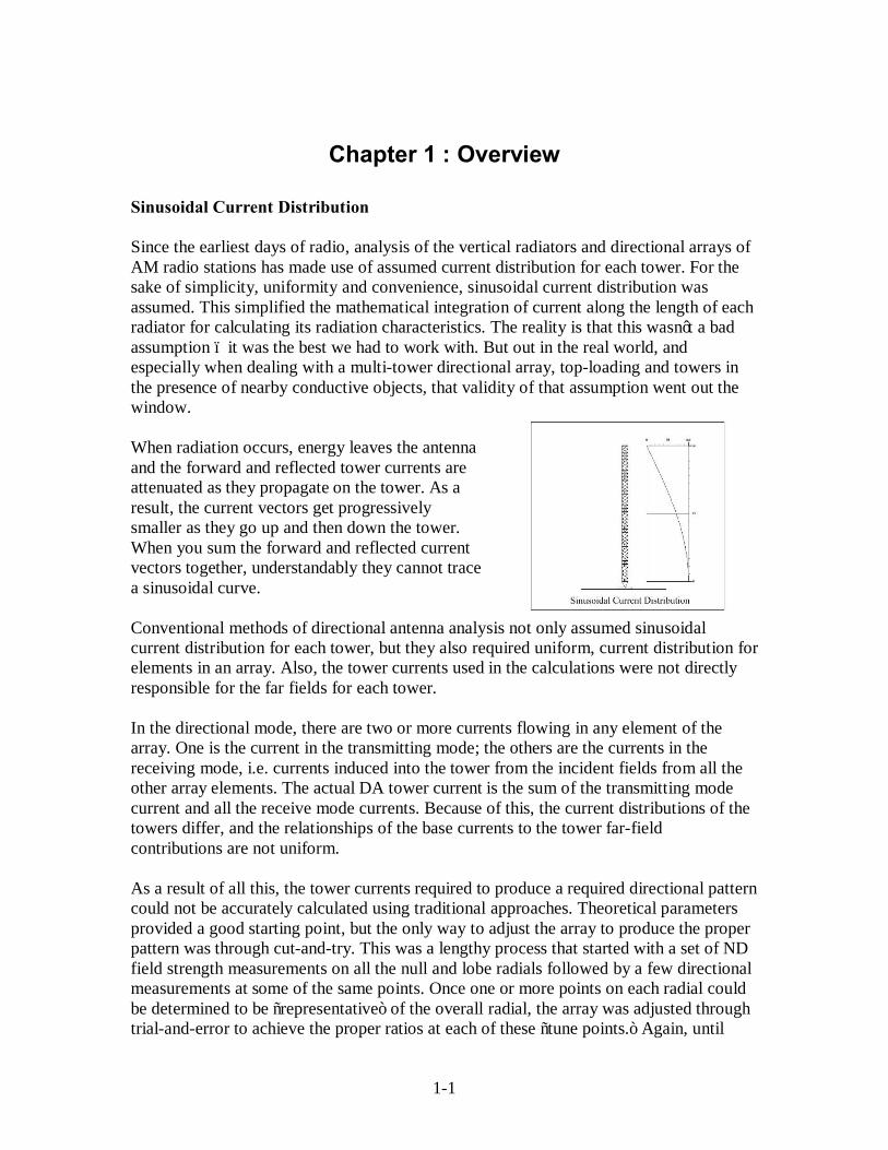
Chapter 1 : Overview Sinusoidal Current Distribution Since the earliest days of radio, analysis of the vertical radiators and directional arrays of AM radio stations has made use of assumed current distribution for each tower. For the sake of simplicity, uniformity and convenience, sinusoidal current distribution was assumed. This simplified the mathematical integration of current along the length of each radiator for calculating its radiation characteristics. The reality is that this wasn’t a bad assumption – it was the best we had to work with. But out in the real world, and especially when dealing with a multi-tower directional array, top-loading and towers in the presence of nearby conductive objects, that validity of that assumption went out the window. When radiation occurs, energy leaves the antenna and the forward and reflected tower currents are attenuated as they propagate on the tower. As a result, the current vectors get progressively smaller as they go up and then down the tower. When you sum the forward and reflected current vectors together, understandably they cannot trace a sinusoidal curve. Conventional methods of directional antenna analysis not only assumed sinusoidal current distribution for each tower, but they also required uniform, current distribution for elements in an array. Also, the tower currents used in the calculations were not directly responsible for the far fields for each tower. In the directional mode, there are two or more currents flowing in any element of the array. One is the current in the transmitting mode; the others are the currents in the receiving mode, i.e. currents induced into the tower from the incident fields from all the other array elements. The actual DA tower current is the sum of the transmitting mode current and all the receive mode currents. Because of this, the current distributions of the towers differ, and the relationships of the base currents to the tower far-field contributions are not uniform. As a result of all this, the tower currents required to produce a required directional pattern could not be accurately calculated using traditional approaches. Theoretical parameters provided a good starting point, but the only way to adjust the array to produce the proper pattern was through cut-and-try. This was a lengthy process that started with a set of ND field strength measurements on all the null and lobe radials followed by a few directional measurements at some of the same points. Once one or more points on each radial could be determined to be “representative” of the overall radial, the array was adjusted through trial-and-error to achieve the proper ratios at each of these “tune points.” Again, until

1-2

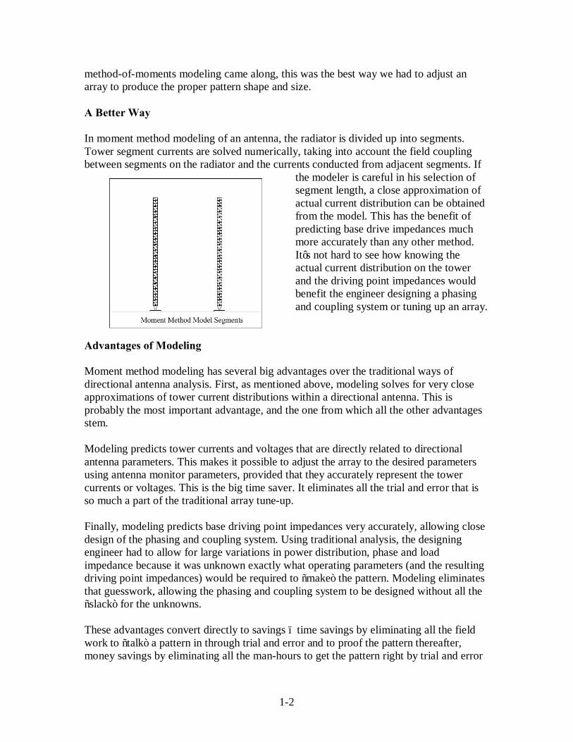
method-of-moments modeling came along, this was the best way we had to adjust an array to produce the proper pattern shape and size. A Better Way In moment method modeling of an antenna, the radiator is divided up into segments. Tower segment currents are solved numerically, taking into account the field coupling between segments on the radiator and the currents conducted from adjacent segments. If

the modeler is careful in his selection of segment length, a close approximation of actual current distribution can be obtained from the model. This has the benefit of predicting base drive impedances much more accurately than any other method. It’s not hard to see how knowing the actual current distribution on the tower and the driving point impedances would benefit the engineer designing a phasing and coupling system or tuning up an array.

Advantages of Modeling Moment method modeling has several big advantages over the traditional ways of directional antenna analysis. First, as mentioned above, modeling solves for very close approximations of tower current distributions within a directional antenna. This is probably the most important advantage, and the one from which all the other advantages stem. Modeling predicts tower currents and voltages that are directly related to directional antenna parameters. This makes it possible to adjust the array to the desired parameters using antenna monitor parameters, provided that they accurately represent the tower currents or voltages. This is the big time saver. It eliminates all the trial and error that is so much a part of the traditional array tune-up. Finally, modeling predicts base driving point impedances very accurately, allowing close design of the phasing and coupling system. Using traditional analysis, the designing engineer had to allow for large variations in power distribution, phase and load impedance because it was unknown exactly what operating parameters (and the resulting driving point impedances) would be required to “make” the pattern. Modeling eliminates that guesswork, allowing the phasing and coupling system to be designed without all the “slack” for the unknowns. These advantages convert directly to savings – time savings by eliminating all the field work to “talk” a pattern in through trial and error and to proof the pattern thereafter, money savings by eliminating all the man-hours to get the pattern right by trial and error

1-3

and the labor required to produce a traditional directional proof of performance based on field measurements, and money savings by allowing proper component selection at design time. Another advantage is the fixed cost represented by the modeling option. A traditional directional antenna tune-up and proof is an open-ended process. At the outset, no one knows how long it will take or how much it will cost because there is no way to know how many iterations it will take to get the pattern right. If there are reradiators or other factors that distort the measured field, months or even years can be added to the process. All this is eliminated through modeling. We all have to do more with less these days. The time and cost savings represented by the modeling option makes this a very attractive choice indeed.

2-1

Chapter 2 : Limitations of Traditional Field Strength Measurements

Since the very beginning, broadcast engineers have employed field strength measurements as a means of verifying the performance of AM antenna systems, non-directional and directional. Indeed, this has been the only means we had to gain some assurance that an antenna was performing as it should. But also since the very beginning, we have known that there are big problems with field strength measurements used for this purpose. Anyone who has made radial field strength measurements on an AM station knows that there is often no rhyme nor reason to their values. In a perfect world, we would see an E x D relationship from the tower to the end of the radial, or at the very worst an E x D relationship modified for changes in ground conductivity. But we don’t live in a perfect world. Measurements plotted on a piece of log-log graph paper often better resemble a shotgun blast than any kind of inverse distance line or conductivity curve. There are many reasons for this, some understandable and others that are tough to quantify. The field intensity measurements that have been traditionally used to verify AM antenna performance are, in reality, magnetic field measurements that are presumed to relate in a certain way to the real parameter of interest, the electric field. Maxwell’s Equations Maxwell’s field equations, derived from Faraday’s Induction Law, Ampere’s Rule and the Biot-Savart Law, show the basic relationship between electric currents and magnetic fields. These are the same equations that give us the speed of light as 3 x 103 meters per second. These equations describe the relationship between currents and fields. Remember that the currents flowing in an antenna create fields. At a distance from the antenna, those E (electric) and H (magnetic) fields are described by the relationship E = 120πH. Note that Ohm’s law states that Z = E/H, so the impedance of free space is given as 120π or 377 ohms. Once we get some distance from the antenna, this starts to fall apart, however. Radial field intensity measurements simply do not work well in any situation other than over uniform, smooth, high-conductivity terrain. Indeed, in Norton’s 1942 paper, The Calculation of Ground-Wave Field Intensity over a Finitely Conducting Spherical Earth, certain simplifying assumptions are made. Real-world effects such as changes in conductivity, most diffraction effects and discontinuities in dielectric constant are not considered at all. These simplifying assumptions are, however, necessary to the process. Ben Dawson, P.E. wrote in his paper The Inadequacy of Magnetic Field Measurements for Antenna Performance Verification that, “Even the simple case of mixed conductivity with no diffraction and uniform dielectric constant is difficult…”

2-2

As was mentioned above, one of the assumptions is a perfectly conducting plane surface. The far field in such a case would diminish in a 1/R relationship. But there are a couple of problems with that analysis. First, the earth is a sphere, not a plane, and second, the earth is not a perfect conductor and it is not homogenous. Maxwell’s120πH relationship comes from an assumption of a permittivity of 4π x 107 henrys/meter = μ, and a dielectric constant of 1/(36π x 109) farads/meter = e. Because neither the permittivity nor the dielectric constant are in fact constant (they are anything but), it is apparent that the E=120πH relationship is not a good fit beyond a certain distance from the antenna. Magnetic Field Disturbances There are a number of factors that can and do disturb the magnetic field at any given location. Here are just a few:

• Surface layer impedance dielectric discontinuities due to vegetation • Conductivity changes due to soil or other surface geology changes • Dielectric constant changes due to soil or surface geology changes • Conductivity and dielectric constant changes due to bodies of water • Diffraction effects due to topography • Diffraction effects due to rugose topography • Diffraction due to abrupt changes in conductivity/dielectric constant changes • Electric field distortion due to electrically small vertical scatterers • Magnetic field distortion due to finite sized loops of conducting material • Absorption by poor conductor structures (i.e. wet concrete) • Quasi-transmission line or ducting effects by urban streets with parallel rows of

structures • Reflection or multipath effects from slopes of good conductivity soil • Quasi-free space propagation in curving sloped terrain • Near-field effects from arrays of radiators • Localized near-field effects from re-radiators • Layered conductivity effects resulting from 1/R propagation

There are many other possible sources of magnetic field variations that will distort the indication on a field intensity meter in any given location. Analysis of Measured Data To anyone who has done any analysis of measured radial field strength data, it would come as no surprise at all that there is an enormous range of variability – in some cases more than 20 dB – of the relationship between the magnetic and electric fields. That variability one of the primary reasons that we analyze such data graphically. It simply won’t fit any equation on a consistent basis.

2-3

Distribution of measured MW radial field intensity data is not Gaussian. It tends, instead, to be Rayleigh distributed, as do most all other propagation situations, with the bulk of the data to one side of the inverse distance line as opposed to even distribution on both sides. As such, arithmetic analysis of measured data will not in many cases provide a correct answer. Keep in mind that such analysis is trying to solve for two variables – the apparent conductivity and the inverse distance field, and the conductivity variable itself is actually more than one unknown. So the best we can do is plot the measured data on a piece of log-log paper and graphically analyze it to see what curves best fit the data. Clearly this is a “best guess” methodology at best.

3-1

Chapter 3 : Method of Moments Basics This course is not intended to be a comprehensive course on antenna modeling. There are other venues for that, including the excellent ARRL Antenna Modeling Course (www.arrl.org). That course as well as others can give the student a much more in-depth look “under the hood” of the method-of-moments modeling process, including the features of and differences between the many programs and cores available (NEC-2, NEC-4, MININEC in its several versions, etc.). Instead, this course will be limited to those facets of modeling that specifically concern the modeling of AM broadcast antennas and directional arrays. So what does a moment method program do? The short answer is that it solves for the current distribution on a wire based on a numerical solution of an integral equation representation of the electric fields. In other words, at its heart, a method moment program provides the user with an accurate prediction of the current distribution on an antenna. Moment method modeling is based on the premise that an antenna is characterized by a collection of arbitrary thin, straight wires in free space or over a ground plane. The process starts with several assumptions:

• The radius of the wires is very small with respect to the wavelength and the wire length

• The wire must be subdivided into short segments so the radius is assumed small with respect to segment lengths.

• The currents in the wires are axially directed (no circumferential currents on the wires)

In the AM broadcast antenna world, all our work is over a ground plane. Ground planes are accommodated in moment method programs by a process called the “method of images.” Where a wire attaches to the ground plane (i.e. one end of a “wire” has a Z coordinate of zero), a current basis function is automatically added to the wire end point connection to ground. Segmentation and Wire Radius Current distribution is solved by dividing the wire into a number of segments. There are some rules established by the limitations of the NEC and MININEC cores related to segmentation and wire radius:

• Segment length, Δ, should be less than about 0.05 wavelengths and longer than 10-3 wavelengths at the desired frequency.

• Extremely short segments (less than 10-3y) should be avoided.

3-2

• The wire radius, α, should be such that λ/α is greater than 30 and 2π(α/λ) is much less than 1.

• The ratio Δ/α must be greater than about 8. • Segments may not overlap.

The FCC rules for modeling of AM broadcast antennas has some further limitations on segmentation and radius. Except for some large aperture free-standing towers, each tower is represented as a wire “cylinder.”

• The radius of each cylinder must be between 80% and 150% of the radius of a circle with a circumference equal to the sum of the widths (S) of the tower sides (3S/2π).

• There must be no less than one segment per 10 electrical degrees of the tower’s physical height.

There is a practical limit to the maximum number of segments, established by the rules above. Generally speaking, the more segments that are used, the better the “resolution” of the model. However, there is a point of “convergence” beyond which increasing the number of segments will produce no improvement in model accuracy. Most models of broadcast towers of reasonable height will produce good results using between 10 and 20 segments. One quick word about a fundamental difference between NEC (NEC-2, NEC-4, etc.) and MININEC cores. The NEC core puts voltage sources in the middle of the specified segment whereas the MININEC core puts it at the end. This has a very practical effect on AM broadcast antenna models. A NEC model of a broadcast tower with the voltage source placed on segment 1 will, in actuality, have its source placed some distance up the tower whereas a MININEC model will have the source placed at the actual base of the tower. To make a NEC model of a broadcast tower work, it is thus necessary to use a greater number of segments, which will result in smaller segments. The FCC rules require that base calculations must be made for a reference point at ground level or within one electrical degree elevation of the actual feed point. With the one degree restriction, a segment length of no more than two degrees must thus be used for NEC models. Another means of overcoming this NEC limitation without resorting to very short segments is to employ a separate short (less than one electrical degree) wire between ground and the bottom of the tower wire for the base connection.

3-3

One more word about NEC and MININEC. Do not be deceived by the names. MININEC is not a scaled-down version of the NEC core. The MININEC core was originally written so that moment method computations could be made on the mini-computers of that day. Even the slowest and smallest of today’s PCs far exceeds the capabilities of the fastest and biggest computers of the early 1980s. The MININEC core has continued to evolve and represents a computing engine every bit as powerful as its NEC counterpart. Once the program solves for the current distribution on the towers, it can then solve for the impedance at each source (tower base). Directional Antenna Sources Current distribution and impedance are not all we need, however. What we need to properly model a directional array are the voltages and phases of the sources at each tower base. A separate source is required for each element in the array. In the broadcast world, we work with current ratios and phases, not voltages and phases. Ratios and phases of the source voltages and currents are generally not the same as the ratios and phases of the desired field parameters. So what we need is a way to translate the tower current moments to source voltages and phases. Source parameter determination requires summing the current moments of the individual towers with a constant source driving each tower base with the others shorted to ground. The summed current moments are normalized to the reference tower to determine the field parameters. Because the relationships of tower currents to base voltages are linear, linear algebra can be used to determine the source parameters as follows: For a two-tower directional antenna: F1 = V11T11 + V12T12 F2 = V21T21 + V22T22 With tower 1 driven and tower 2 shorted: F1 = T11 F2 = T21 With tower 2 driven and tower 1 shorted: F1 = T21 F2 = T22 For a directional array with n towers: F1 = V11T11 + V12T12... + V1nT1n F2 = V21T21 + V22T22... + V2nT2n .

3-4

.

. Fn = Vn1Tn1+Vn2Tn2... + VnnTnn [F] = [T] x [V] [S] = [T]-1 [V] = [F] x [S] For more information on calculating the voltage source required to produce a particular set of current moments in an array, I recommend J.L. Smith’s excellent book, Basic NEC with Broadcast Application, available at the SBE Store. In the early days of moment method modeling of AM antennas, the consulting engineers who pioneered the use of modeling used iteration to determine the proper source voltages and phases. While this worked, it was very time consuming and not particularly accurate. Today, a series of matrices is used to determine the source parameters to produce the requisite element fields. There are external matrix inversion programs available for this purpose (such as Westberg Consulting’s DRIVE), and at least two commercial MININEC applications (Expert MININEC Broadcast Professional, which is no longer available, and ACSModel) have an internal pattern synthesis routine. Coordinate Systems

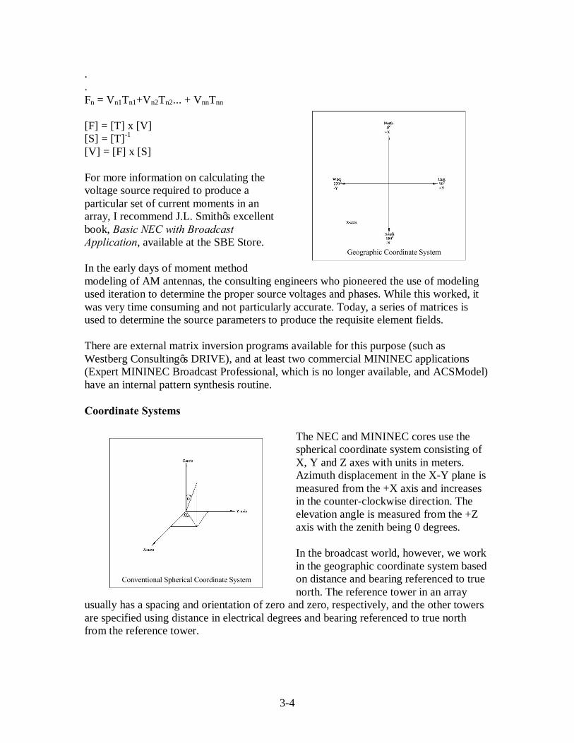
The NEC and MININEC cores use the spherical coordinate system consisting of X, Y and Z axes with units in meters. Azimuth displacement in the X-Y plane is measured from the +X axis and increases in the counter-clockwise direction. The elevation angle is measured from the +Z axis with the zenith being 0 degrees. In the broadcast world, however, we work in the geographic coordinate system based on distance and bearing referenced to true north. The reference tower in an array

usually has a spacing and orientation of zero and zero, respectively, and the other towers are specified using distance in electrical degrees and bearing referenced to true north from the reference tower.

3-5

While some moment method wrappers, such as ACSModel and Expert MININEC Broadcast Professional, will allow entry in the geographic coordinate system, programs which do not will require conversion to the metric X-Y-Z coordinate system. Conversion is not difficult. The reference tower is specified at X-Y coordinates 0,0. The distance to other array elements is then converted from degrees to meters, and the X-Y coordinates are determined using the following equations: X = Spacing cos(θ) Y = Spacing sin(θ) Z axis coordinates are straightforward. Each tower base has a Z coordinate of zero. The Z coordinate of the tower top is simply the tower electrical height in meters. Calibrating the Model To use a moment method model for proofing with internal current or voltage measurements, the model must be “calibrated” by comparing measured base impedances to those predicted by the model. This is done by first making a set of matrix measurements. The base impedance of each tower in the array is measured with all the other towers either floated or shorted, depending on tower height. Shorter towers are generally floated while taller towers are shorted – whichever condition is closest to the “detuned” condition for that height of radiator. The model is then run and changed to account for environmental factors, such as velocity factor, loading of guy wire insulators, etc. The modeled tower height will generally be different (usually greater) than the physical height because of this velocity factor. Generally speaking, larger aperture towers will have lower velocity factors due to the greater number and length of structural cross-members. The modeled tower height and wire radius will be based on the observed impedance matrix. Radiation Pattern Amateur radio experimenters and others who use moment method modeling are primarily interested in two things by way of program output: input VSWR/bandwidth and radiation pattern. In the broadcast engineering world, we don’t really care about VSWR because we employ matching networks at each array element, although the driving point impedances are important for a number of reasons. And while we do care about radiation pattern, the fact is that if we can produce the correct field from each tower in the array, the pattern will be right. Most if not all NEC and MININEC packages have a radiation pattern provision, allowing the user to output the horizontal plane radiation pattern at any elevation. This output is not really of interest to the broadcast array modeler other than as a confirmation that the model has been properly constructed. If, for example, a pattern should have nulls at 45

4-6

and 315 degrees and a lobe at 180, the moment method package radiation pattern output should show that and not something else.

Chapter 4 : FCC Modeling Rules The FCC’s modeling rules are contained in 47 C.F.R. §73.151 and §73.155. The actual text of the rules is available on the FCC’s website at www.fcc.gov, so they are not included herein. Rather, a digest of the new rules is provided herein. In essence:

• A method of moments program must be used. • The model must be constructed in such a manner that it does not violate any of the

internal constraints of the program used. • Only arrays consisting of series-fed elements are eligible for the modeling option. • Matrix impedance measurements must be made at the base and/or feed point of

each array element. • The physical characteristics of array elements (height and radius) may be varied

to calibrate the model. • Model impedances must agree with the measured impedance matrix within ±2

ohms and ±4%. • Actual spacings and orientations must be used. • Towers may be modeled using vertical wires or with multiple wires representing

legs and cross-members. • Drive point impedances must be determined from the model output. • The radius of each array element must be between 80% and 150% of the radius of

a circle with a circumference equal to the sum of the widths of the sides. • No less than one segment per 10 electrical degrees of the tower’s physical height

must be used. • Base calculations must be made at ground level or within one electrical degree of

the actual feed point elevation. • For non-tapered towers, the modeled height of each element must be between

75% and 125% of the physical height. • For tapered towers, stepped-radius wire sections may be used to simulate a

tower’s taper, or the tower may be modeled using wires for the legs and cross-members.

• The series feed impedance between the ATU output and tower base must be less than 10 uH unless measured higher.

• The shunt feed capacitance to model the base region effects must be less than 250 pF unless measured or specified by the manufacturer to be higher.

• If the shunt feed capacitive reactance is less than five times the magnitude of the base operating impedance, it must be considered in the model.

• The tower positioning must be confirmed post-construction by a surveyor or registered professional engineer.

• Operating parameters must be determined from the output of the computer model.

4-2

• Samples may be current transformers or voltage sampling devices at the base of each element, or tower-mounted loops.

• Loops must be located at the elevation where the current in the tower would be at a minimum if the tower were detuned.

• Loops may be used only on towers of identical cross-sectional structure, including leg and cross-members.

• Loops on unequal height towers must be mounted with identical orientations at the proper elevations.

• If tower heights other than the physical heights are used in the model, loops must be mounted at the same percentage height as indicated in the model.

• Sample lines must be equal in length within one electrical degree and characteristic impedance within two ohms, as confirmed by measurement.

• Base current sample transformers may be used for towers of 120 degrees or less or 190 degrees or greater in height.

• Base voltage sample devices may be used for towers of greater than 105 electrical degrees.

• Tower-mounted sample loops may be used on towers of any height. • Base current sample transformers or voltage sampling devices must be calibrated

against one another within the manufacturer’s specifications. • Antenna monitor sample indications must agree with the model-determined ratios

within ±5% and with the model-determined phases within ±3 degrees. • Three reference field strength measurements must be made on each pattern

minima and maxima radial. More detail on the FCC rules regarding calibration and certification of the sample system and the required biennial recertification thereof are presented in the tutorial on field procedures for AM moment method modeling.

5-1

Chapter 5 : Using Moment Method Modeling for Directional Antenna Proofs

Benefits of Modeling There are many reasons why using moment method modeling for tune-up and performance verification of AM directional antennas is superior to traditional methods. We have covered most of these in prior sections of this course. Among them are:

• Accurate locations for tower-mounted sample loops • Accurate driving point impedance data for every array element • Accurate pre-construction bandwidth analysis • Eliminating dependence on field measurements for accurate adjustment

The bottom line, though, is cost savings. With more accurate data going in, without the open-ended prospect of trial-and-error adjustment and without the requirement for hundreds of non-directional and directional field measurements, the DA tune-up/proof project employing moment method modeling will have much lower expenses and a more-or-less fixed cost. A direct benefit of lower, fixed costs is better compliance. It stands to reason that station licensees that would otherwise opt to roll the dice on an inspection, notice of violation and forfeiture for having an array out of tolerance because of the often huge costs of bringing it into compliance, would be more inclined to spend a much lower and fixed amount to eliminate that risk. That, in turn, results in reduced interference, which benefits everyone on co- and adjacent-channels. Facility and Model Eligibility The FCC rules now permit moment method modeling as a means of performance verification of AM directional arrays in certain cases. A digest of these rules is contained in another section of this course. To be eligible for the modeling proof option, a facility and model must meet the following criteria:

• Only series-fed antenna elements • Only accurate current/voltage samples • The moment method model must match the measured base Z matrix • For cylinder models, the effective radius assumption is limited to 80%-150% of

the physical radius • For cylinder models, the effective height assumption is limited to 75%-125% of

the physical height • At least one segment for each 10 degrees of physical height

5-2

• The model feedpoint must be at ground level or within one degree of physical elevation

• Series inductance must be 10 uH or less unless measured higher • Parallel stray capacitance must be 250 pF or lower unless measured higher

Modeling Software While the FCC rules do not specify a modeling platform, and while good results can be obtained from any platform employing a NEC or MININEC core, the FCC Media Bureau has opted to use Expert MININEC Broadcast Professional (hereinafter “MBPro” and reportedly no longer in production) and ACSModel (available from the SBE Store at http://www.sbe.org/sections/store_books_listings.php or directly from Au Contraire Software at http://www.aucont.com) . Employing the same platforms as the FCC will ensure comparable results, presumably reducing processing delays. Examples in this course were taken from both ACSModel and MBPro v. 14.5.

6-1

Chapter 6 : Measurements for Moment Method Modeling of AM Arrays

Base Impedance Matrix Measurements The one thing that differentiates a typical moment method antenna model and an AM broadcast directional array moment method model is that the latter is calibrated against real-world conditions. This calibration process removes some of the assumptions, moving them from the realm of the unknown to the known. We can assume a velocity factor for a tower, for example, because the modeled tower height at a certain effective height behaves the same as the prototype tower in the real world. Precedent to construction of a method moment model, then, is a set of base impedance matrix measurements. The procedure for making these measurements is presented in detail here with the assumption that the one making the measurement knows how to operate his test equipment, presumably a General Radio 1606B or equivalent impedance bridge or Delta Operating Impedance Bridge (OIB) in one of its forms, and either with a suitable signal generator and detector. Sample System Measurements Once the model has been constructed, calibrated and run, the sample system must be calibrated – proofed – before the directional array can be adjusted to the model parameters. The FCC has set certain guidelines for the lengths and impedance of sample lines, sample current transformer accuracy and loop dimensions and orientation. All these are covered in the chapter FCC Modeling Rules in the Modeling tutorial within this course. If you have not yet read that chapter, you are encouraged to do so now because the material therein is foundational to much of what will be presented in this tutorial. The base impedance matrix measurements are requisite to model construction and are essentially a one-time affair. Unless something changes on one of the towers – the addition of an STL antenna or replacement of an isocoupler with a different type, for example – there is no reason to repeat them. The sample system measurements, on the other hand, are a biennial event. The FCC requires that the station licensee “…recertify the performance of that directional pattern at least once within every 24 month period” including measurements “…made to verify the continuing integrity of the antenna monitor sampling system.” This requirement has proven to be a bit off-putting to some engineers, but this is more because of a lack of understanding of the requirements than any particularly difficult aspect of the recertification. The reality is that the recertification measurements need consist of nothing more than spot-checks of the information that was found in the full certification when the array was

6-2

tuned up. For example, the sample lines must be measured to determine their resonant frequency and characteristic impedance. Much of the work in this regard is in finding the unknowns. Once certified, those variables have been solved. Recertification can be done by simply measuring the impedance of the open-circuited sample lines at the frequencies on which they were found to be resonant and confirm that they are still resonant. Characteristic impedance measurements can likewise be quick measurements on two frequencies, one above and one below the resonant frequency, which were determined in the initial system proof. The entire sample system of even a large array can be measured in a few hours. While there is certainly nothing wrong with hiring a consulting engineer to do the recertification, any competent RF engineer who can operate a bridge can do it; the biennial recertification is well within the capabilities of most AM station chief engineers. Reference Field Strength Measurements The FCC’s AM modeling rules require that: “Reference field strength measurement locations shall be established in directions of pattern minima and maxima.” In essence once the pattern has been adjusted to the model parameters, three radial field strength measurements must be made on each of the null and lobe radials. These measurements must be repeated during the biennial recertification. It should be stressed that these reference field strength measurements are not “monitor points”; there are no licensed maxima applied to them and there is no need to measure the field strength at any of the points between biennial recertifications. Further, if, during the recertification measurements, one or more of the measurements is found to exceed the original values, it means nothing. The measurements were included in the rules simply to give the licensee a means of verifying the gross pattern shape and size. If measurement of the reference field strength points were to show, for example, an overall shift in the pattern (some fields up and others down), that might be an indication of another problem… but then again, it might not. There is no statutory duty to act on a changed reference field strength. We will not cover in this course the reference field strength measurements beyond this brief discussion. It is assumed that the engineer responsible for the care and feeding of an AM directional array is well acquainted with the proper operation of a field intensity meter and the selection of good radial measurement point locations. The measurements described above will be fully discussed in chapters 7 and 10 herein.

7-1

Chapter 7 : Matrix Impedance Measurements We will deal with field measurements of impedance in more detail in the tutorial on field work for moment method modeling for performance verification, but a brief discussion of the requirements is needed here. The term “base impedance matrix” sounds complicated and perhaps a bit off-putting to the engineer new to modeling, but the opposite is actually true. Measurement of the base impedance matrix consists of nothing more frightening than bridging the base of each tower with all the other towers either floated or shorted. Measuring at the ATU output or the tower base itself is optional, and many modelers measure both, but the general rule is that if you are base sampling (from a current or voltage sample device at the ATU output), you must measure the matrix at the ATU output. Loop sampled towers should be measured at the base itself. In the simple case of a two-tower array employing 90-degree towers, start with tower 1. Assuming that measurements will be made at the base of each tower, disconnect all appurtenances from both towers, including isocouplers, lighting chokes, sample lines, feed tubing and the like, watching out for unwanted capacitive coupling (such as a disconnected sample line still lying in close proximity to a tower member). With the base of tower 2 now open, back at tower 1, bridge the base of the tower right at the top of the base insulator, at the point where the feed tubing would normally connect, and note the resistance and reactance (remember to correct the reactance for frequency), marking the notation as taken with tower 2 open. If desired, now short tower 2 with at least two low-inductance straps made from copper strap or 1-inch or wider braid. Short directly across the base insulator to the RF ground under the insulator. Repeat the base impedance measurement at tower 1 and note the R and X, correcting the X for frequency. Be sure to note that tower 2 was shorted. Then reverse the process. Open tower 1 and bridge the base of tower 2. Then short tower 1 and bridge the base of tower 2. That’s it, a complete set of base impedance matrix measurements. If there are more towers in the array, continue with this process, measuring the base impedance of each tower in turn with all the other towers either floated or shorted. What is the criterion for measuring with the unused towers open or floating? A good rule of thumb is to employ the condition that would best approximate a “detuned” condition for the tower. Electrically short towers, say less than 120 electrical degrees, are better floated while electrically tall towers, say more than 150 electrical degrees, are better shorted. Towers of intermediate heights should be both open and shorted in the matrix. As the model is run, the condition that the model best matches can be used to calibrate the model.

7-2

What is the criterion for measuring at the tower base versus at the ATU output? For arrays employing loop sampling, if it is possible to measure at the tower base with the feed tubing completely disconnected, it is better to do so because it eliminates the several unknown variables of series and shunt stray reactance. Those reactances can often be measured separately and dealt with outside the model structure. In many cases, however, the feed tubing has been welded or otherwise electrically bonded to the tower structure, and removing it would be difficult. In such cases, measure at the ATU output. The strays can still be measured with some degree of accuracy and treated outside the model.

8-1

Chapter 8 : A Step-by-Step Moment Method Modeling Example (MBPro)

Constructing the Model We’ll start with a simple but typical directional array. It is a three-tower inline array with 77-degree, 18-inch face triangular towers spaced 75.9 degrees apart. This is a good example to learn the basics with. The principles and procedures learned here will be applied to other examples later. Getting Started With all the details of the directional array in hand, including element spacing, orientation, height, ratio, phase, tower face width, tower configuration and impedance matrix, the next step is to construct the model. Run MBPro and click File | New. Later versions will prompt for whether this is a general or broadcast antenna. Click broadcast antenna. Next you will be prompted for a project description. Enter any pertinent informational data. The information entered here will be printed on each page of the output. For our example, enter: KLVZ 3-Tower Daytime Array 810 kHz, 2.2 kW If your version does not bring up the general/broadcast antenna prompt, you will be taken directly to the project description. It will then be necessary to set the units and coordinate system (others can skip these steps). Click Problem Definition | Geometry | Dimensions, Environments, Coordinates. For dimensions, select “degrees”; for coordinates, select “geographic”; for environment, select “perfect ground.” Next, click Problem Definition | Electrical | Frequency (or click ctrl-f). Set the units to kHz, set the initial frequency to 810, then click Modify and OK. Geometry Nodes With the preliminaries out of the way, now it’s time to construct the actual model. Click Problem Definition | Geometry | Geometry Points (or click ctrl-n). Our tower geometry is as follows: Twr. Spacing Orientation Height 1 75.9 220 77 2 0 0 77 3 75.9 40 77

8-2

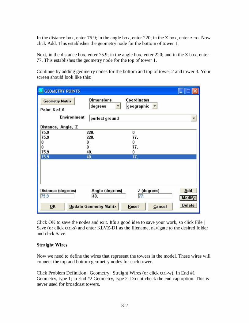
In the distance box, enter 75.9; in the angle box, enter 220; in the Z box, enter zero. Now click Add. This establishes the geometry node for the bottom of tower 1. Next, in the distance box, enter 75.9; in the angle box, enter 220; and in the Z box, enter 77. This establishes the geometry node for the top of tower 1. Continue by adding geometry nodes for the bottom and top of tower 2 and tower 3. Your screen should look like this:

Click OK to save the nodes and exit. It’s a good idea to save your work, so click File | Save (or click ctrl-s) and enter KLVZ-D1 as the filename, navigate to the desired folder and click Save. Straight Wires Now we need to define the wires that represent the towers in the model. These wires will connect the top and bottom geometry nodes for each tower. Click Problem Definition | Geometry | Straight Wires (or click ctrl-w). In End #1 Geometry, type 1; in End #2 Geometry, type 2. Do not check the end cap option. This is never used for broadcast towers.

8-3

Now we need to enter the radius. Start with a nominal radius of 3T/2π. Convert the face width, T, to meters. 18” / 39.36 = 0.457 meters. (3 x 0.457) / (2 x π) = .2188 meters. Enter 0.2188 for the radius. Next, we need to decide the number of segments. The FCC rules call for not less than one segment per ten electrical degrees, so the minimum number of segments is 8. An experienced modeler would likely start with that minimum and run a convergence test to determine the point of diminishing returns with regard to increasing the number of segments. For now, enter 20 in the Number of Segments box. 20 Segments meets all of the rules and provides good convergence. In fact, 20 segments works reasonably well for most broadcast antenna modeling applications. Click Add to create the wire. Repeat this operation for tower 2. Enter 3 and 4 in the End #1 and End #2 Geometry boxes, respectively. Enter 0.2188 in the Radius box, 20 in the Number of Segments box and click Add to create the wire. Repeat for tower 3, entering 5 an 6 in the Geometry boxes and duplicating all the other information before clicking Add. Your screen should look like this:

Click OK to close the Straight Wires entry window. Click ctrl-s to save your work.

8-4

Calibrate the Model The next step involves either floating or shorting two of the towers and driving the other to get a look at the impedance compared with the base impedance matrix for that same condition. In this case, because the towers are electrically short, the matrix was measured with the towers floated (open), so we will need to insert an open circuit at the base of two of the towers at a time. In MININEC, wires with one end at a Z value of 0 are presumed to be connected to ground (shorted), so we have to do something to lift that ground. We do this with a lumped load. Click Problem Definition | Electrical | Lumped Loads (or type ctrl-l). Click List Current Nodes to see the list of nodes. Note that node 1 (with a Z axis value of 0) is the base of tower 1, node 21 is the base of tower 2 and node 41 is the base of tower 3. We want to place an open circuit at the bases of towers 1 and 3, the end towers. The easiest way to do this is to enter a very high capacitive reactance at the nodes for the bases of those towers. In the Load current node box, enter 1 for the base of tower 1. In the Resistance box, enter 0. In the Reactance box, enter -10000. This value is not critical. It needs to be a high enough reactance that no significant amount of current will flow through it at toperating frequency. Click Add to add the load. Repeat this for node 41 for the base of tower 3. Your screen should look like this:

Click Ok to close the screen. Save your work. Now we need to drive tower 2 with a voltage source. Click Problem Definition | Electrical | Voltage/current sources (or type ctrl-v). The program defaults with a source at node 1. Type 21 in the Source current node box. The Sector box should default to 1. In the Magnitude box, type 1. This is not critical; any convenient value will work. The Phase box should default to zero. Click Modify. Your screen should look like this:

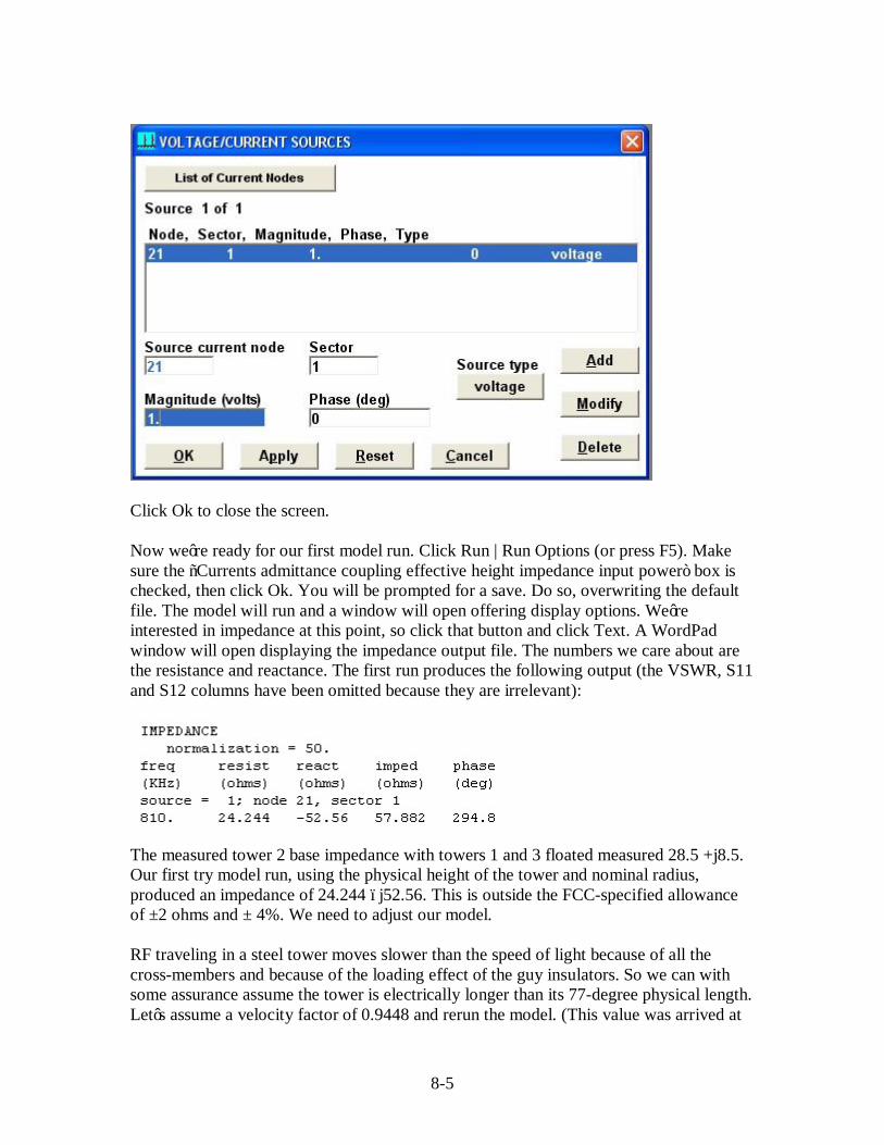
8-5

Click Ok to close the screen. Now we’re ready for our first model run. Click Run | Run Options (or press F5). Make sure the “Currents admittance coupling effective height impedance input power” box is checked, then click Ok. You will be prompted for a save. Do so, overwriting the default file. The model will run and a window will open offering display options. We’re interested in impedance at this point, so click that button and click Text. A WordPad window will open displaying the impedance output file. The numbers we care about are the resistance and reactance. The first run produces the following output (the VSWR, S11 and S12 columns have been omitted because they are irrelevant):

The measured tower 2 base impedance with towers 1 and 3 floated measured 28.5 +j8.5. Our first try model run, using the physical height of the tower and nominal radius, produced an impedance of 24.244 –j52.56. This is outside the FCC-specified allowance of ±2 ohms and ± 4%. We need to adjust our model. RF traveling in a steel tower moves slower than the speed of light because of all the cross-members and because of the loading effect of the guy insulators. So we can with some assurance assume the tower is electrically longer than its 77-degree physical length. Let’s assume a velocity factor of 0.9448 and rerun the model. (This value was arrived at

8-6

after several iterations. Finding the right number is a sometimes lengthy trial and error process. The intermediate steps are omitted here in the interest of brevity.) Click ctrl-n to look at the nodes again. Modify each tower top node to have a Z of 81.5 degrees (77 / 0.9448), then click Ok. 81.5 degrees is within the 75%-125% of physical height limit. Type F5, select “Currents admittance coupling...” and click Ok. You will be prompted for another save. During the process of determining the correct velocity factor/height, experienced modelers often change the file name slightly so that they can go back to a particular configuration without manually modifying the geometry nodes. When the Display Options window comes up, again click Impedance and Text to see the calculated impedance at the base of tower 2 with towers 1 and 3 floated.

Note that the impedance is now shown as 28.6 –j27.9. The resistance is within the ±2-ohm/±4% window. In fact, it’s almost dead on the matrix value of 28.5. But the reactance is off. Remember that the FCC rules allow a series inductance of up to10 uH. If we assume a series reactance of the opposite of +j8.5+-j27.9 (+j36.4), the model output impedance for tower 2 driven with towers 1 and 3 floated becomes 28.6 +j8.5, very close to the measured value. 36.4 / 2PiF = 7.2 uH, within the allowable 10 uH limit. Next, we need to drive tower 1 and float towers 2 and 3. Type ctrl-l to bring up the lumped loads window. Click on the node 1 load, click in the Load current node box, change it to 21 and click Modify and Ok. That action got rid of the open at the base of tower 1 and moved it to the base of tower 2. Now we need to move the voltage source to the base of tower 1. Click ctrl-v to bring up the Voltage/current sources window. In the Source current node window, type 1, click Modify and Ok. Now we’ll run the model again. Press F5, select “Currents admittance coupling...” and click Ok. You will be prompted for another save. Change the file name to indicate that this is tower 1 driven with 2 and 3 floated and click Save. When the Display Options window comes up, click Impedance and Text.

Note that the impedance from the model run is shown to be 29.3 –j27.0. The matrix impedance for tower 1 with tower 2 and 3 open measured 29.0 +j7.0, so this value of R is

8-7

within the ±2 ohm/±4% window. If we add a series reactance of +j34.0, the reactance component becomes +j7.0, right on the nose. Again +j34 corresponds to an inductance value of less than the 10 uH FCC maximum, so we’re good. Now we repeat the exercise by changing the node of the lumped load at the base of tower 3 (node 41) to the base of tower 1 (node 1). Then move the voltage source from node 1 to node 41, rerun the model, save with a different file name and look at the impedance for tower 3 driven with towers 1 and 2 floating.

The impedance is shown to be 29.3 –j27.0. The matrix Z of tower 3 driven with towers 1 and 2 open measured 29.0 +j7.0. The predicted R is within the ±2-ohm/±4% window, so it’s fine. If we use a series impedance of +j34.0, we get an X of +j7.0, right on the money. We can now consider our model to be calibrated. In some cases, it could be that once we get the first tower calibrated to the model and run the second tower with the others floated or shorted, the R is outside the ± 2-ohm/±4% window. It may then be necessary to adjust the height of the driven tower a bit to bring the R within the window. Once that is done, the bad news is that you get to re-run the previous tower again with the changed height on the second tower. That tower may now need a tweak as well. Then, if the first tower is changed, the second tower must be re-run and perhaps adjusted again. The process repeats with all the towers in the array until the full matrix is matched. This can be a time-consuming process, so be patient. An experienced modeler quickly gains a “feel” for what effect each parameter has, speeding the iteration process considerably. Radius Change Another tool in the box is tower radius, which affects the R to X ratio a bit. You won’t see a lot of change in most cases by changing the radius, but it does sometimes, in combination with height changes, allow you to bring the R and the X into tolerance with the matrix measurements. For a typical radiator, a change in effective height makes a substantial change in base impedance. Consider the following, calculated at 833 kHz (where 1 degree = 1 meter): G = 92m, Zbase = 49.3 +j30.3

8-8

G = 100m, Zbase = 69.4 +j 65.0 G = 105m, Zbase = 86.4 +j89.7 A radius change makes a much smaller change in impedance. For the 92m case above: R = 0.8m, Zbase = 48.3 +j30.9 R = 1.0m, Zbase = 49.3 +j30.3 R = 1.25m, Zbase = 50.5 +j29.6 Still, varying the radius in conjunction with the effective height can be a good tool to bring the model into calibration. Tapered Towers The FCC rules make provision for tapered towers such as free-standing structures or Blaw-Knox type “diamond” structures to be modeled using many wires to represent legs and cross members. As you can imagine, this would require a great deal of work to simply set up the initial model. You can forget about the geographical coordinate system in such a complex model. Every wire representing each leg, horizontal and diagonal member would have to be described by a set of spherical (X-Y-Z) coordinates for each end point with a straight wire between them. And once the model is created, it would be very difficult to calibrate it – you would have to just about start over to make any change in the effective height or radius. There are, however, other, simpler options that work well for many tapered tower situations. One involves using a “Michelin Man” approach, employing wires of different radii to represent different cross-sections of the tower. For example, near the base of a typical free-standing tower with a face width of, say, 20 feet, a radius of 2.8 meters might be used for the first 20 feet of height. The center of the next 20 foot span might have a radius of, say, 15 feet, so another wire would be used with a radius of 2.2 meters. The process would repeat itself up the tower. A much longer wire might me used for the upper portion of the tower if its taper is minimal or non-existent. One caveat about using multiple wires on a radiator: It is important that the segment length on all the wires be close to the same. For example, let’s say that in the above example the overall tower height is 90 degrees. If this were being modeled with one wire, we would likely use 20 segments for the entire tower. If the frequency is 810 kHz, each segment would be about 15 feet long. But if we’re going to break up the tower into 20-foot segments for the purpose of simulating taper with stepped radii, we will need at least two segments per wire, making each segment 10 feet in length. When we get to the longer wires representing the untapered portion near the top, we must choose a number of segments that will result in a segment length of close to ten feet. Maintaining uniform segment length is critical to good model performance. Another approach to tapered towers is to assume an “average” radius for the entire structure. This approach works satisfactorily for lightly tapered towers, those with

8-9

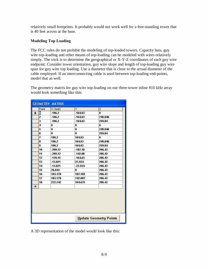
relatively small footprints. It probably would not work well for a free-standing tower that is 40 feet across at the base. Modeling Top Loading The FCC rules do not prohibit the modeling of top-loaded towers. Capacity hats, guy wire top-loading and other means of top-loading can be modeled with wires relatively simply. The trick is to determine the geographical or X-Y-Z coordinates of each guy wire endpoint. Consider tower orientation, guy wire slope and length of top-loading guy wire span for guy wire top loading. Use a diameter that is close to the actual diameter of the cable employed. If an interconnecting cable is used between top-loading end-points, model that as well. The geometry matrix for guy wire top-loading on our three-tower inline 810 kHz array would look something like this:

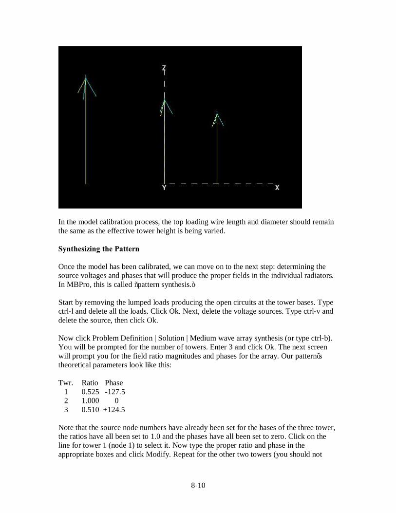
A 3D representation of the model would look like this:

8-10

In the model calibration process, the top loading wire length and diameter should remain the same as the effective tower height is being varied. Synthesizing the Pattern Once the model has been calibrated, we can move on to the next step: determining the source voltages and phases that will produce the proper fields in the individual radiators. In MBPro, this is called “pattern synthesis.” Start by removing the lumped loads producing the open circuits at the tower bases. Type ctrl-l and delete all the loads. Click Ok. Next, delete the voltage sources. Type ctrl-v and delete the source, then click Ok. Now click Problem Definition | Solution | Medium wave array synthesis (or type ctrl-b). You will be prompted for the number of towers. Enter 3 and click Ok. The next screen will prompt you for the field ratio magnitudes and phases for the array. Our pattern’s theoretical parameters look like this: Twr. Ratio Phase 1 0.525 -127.5 2 1.000 0 3 0.510 +124.5 Note that the source node numbers have already been set for the bases of the three tower, the ratios have all been set to 1.0 and the phases have all been set to zero. Click on the line for tower 1 (node 1) to select it. Now type the proper ratio and phase in the appropriate boxes and click Modify. Repeat for the other two towers (you should not

8-11

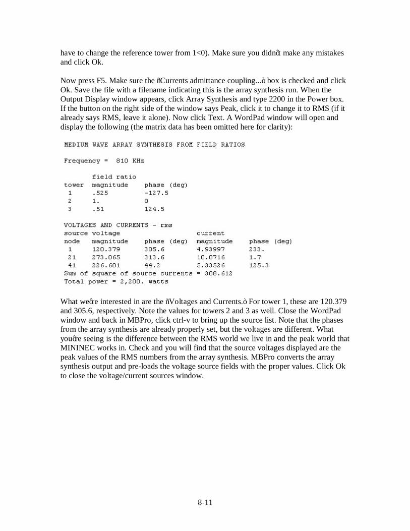
have to change the reference tower from 1<0). Make sure you didn’t make any mistakes and click Ok. Now press F5. Make sure the “Currents admittance coupling...” box is checked and click Ok. Save the file with a filename indicating this is the array synthesis run. When the Output Display window appears, click Array Synthesis and type 2200 in the Power box. If the button on the right side of the window says Peak, click it to change it to RMS (if it already says RMS, leave it alone). Now click Text. A WordPad window will open and display the following (the matrix data has been omitted here for clarity):

What we’re interested in are the “Voltages and Currents.” For tower 1, these are 120.379 and 305.6, respectively. Note the values for towers 2 and 3 as well. Close the WordPad window and back in MBPro, click ctrl-v to bring up the source list. Note that the phases from the array synthesis are already properly set, but the voltages are different. What you’re seeing is the difference between the RMS world we live in and the peak world that MININEC works in. Check and you will find that the source voltages displayed are the peak values of the RMS numbers from the array synthesis. MBPro converts the array synthesis output and pre-loads the voltage source fields with the proper values. Click Ok to close the voltage/current sources window.

8-12

Now we have to re-run the model with the new sources. Later versions of MBPro will bring up a window after the array synthesis has run reminding you of this. Press F5, make sure the “Currents admittance coupling...” box is checked and click Ok. You will be prompted for a file save. Change the name to reflect that this run has the correct DA source voltages and phases and save. When the Output Display window appears, click Impedance and Text. A WordPad window will open displaying the base driving point impedances for the array.

Print this page. Those numbers, once modified for the series inductance values that we determined for each tower in the calibration process, will become the driving point impedances for the towers. Keep in mind here that these numbers are for the tower bases. If there are significant amounts of stray capacitance, that must be considered and factored into the driving point impedance seen at the output of the antenna tuning units. More on that later.

8-13

Close the WordPad window. In the Output Display window, click Current Moments and Text. A WordPad window will open displaying the current moments for the array. If desired, divide the current magnitude value for the two end towers by that for the reference tower to confirm that the field ratios are correct. Check the phases to make sure they are correct as well. Close the WordPad window.

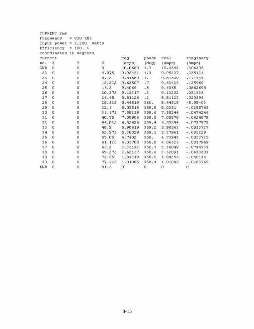
Next, on the Display Options window, click Currents. You should see something like this. Note the magnitude and phase at the base node of each tower (1, 21 and 41). These, normalized to the values for tower 2 (reference tower), become the operating parameters for the array if you are employing base sampling.

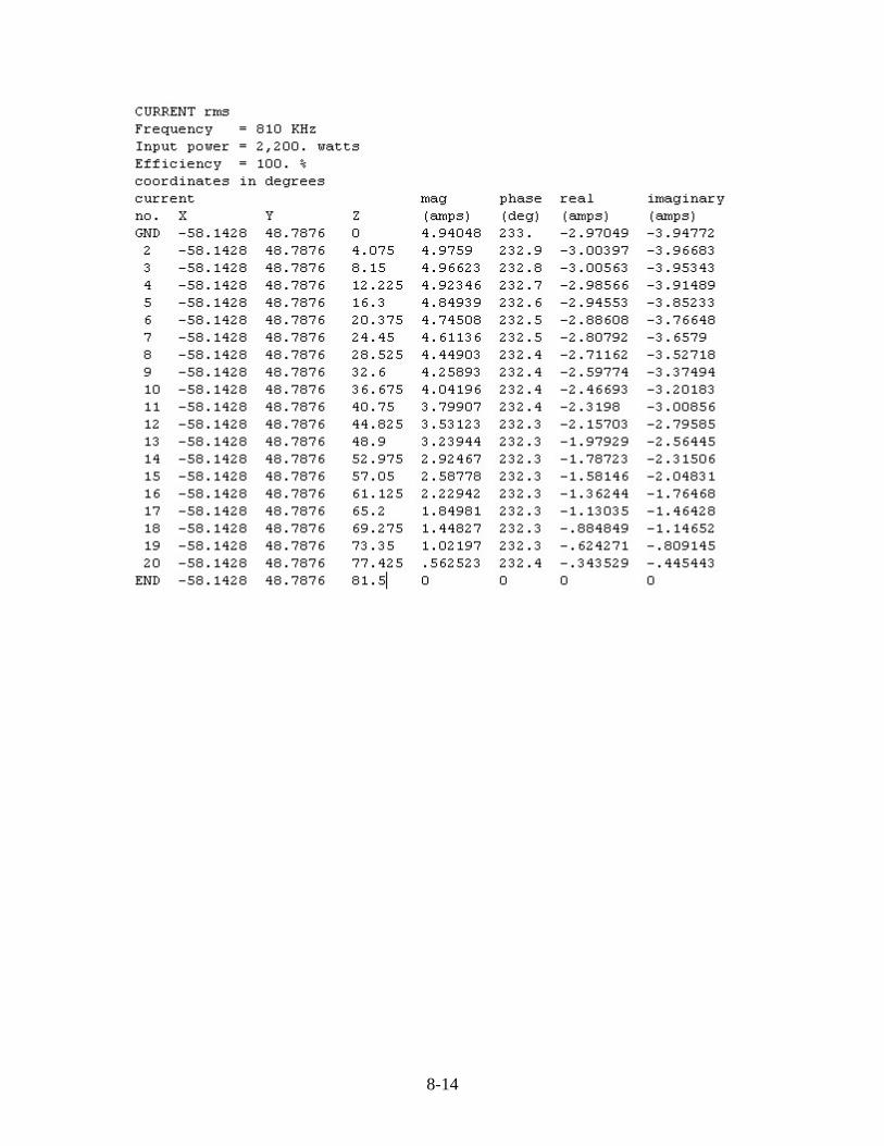
8-14

8-15

8-16

The base magnitudes and phases are listed as: Twr. Mag. Phase 1 4.94 233.0 2 10.07 1.7 3 5.33 125.3 Normalized to the reference tower, the base operating parameters become: Twr. Ratio Phase 1 0.491 -128.7 2 1.000 0.0 3 0.529 +123.6 As with the driving point impedances above, remember that these numbers are at the tower base. If there is a significant amount of stray capacitance, it must be considered outside the model to determine the effect on the impedance, current and phase at the ATU output. The base driving point impedance is modified by a shunt capacitive and series inductive reactance as follows:

8-17

RA = RBXS

2/(RB2+(XB+XS)2)

XA = +jXS(RB2+XB

2+XBXS)/(RB2+(XB+XS)2)+jXL

Where: ZBASE = RB +jXB ZATU = RA +jXA XS = Shunt reactance XL = Inductive series reactance The ATU output current and phase are modified by a shunt capacitive reactance as follows: IATU Magnitude = ((1 + XB/XS)2 + (RB/XS)2)1/2 IATU Angle = arctan(-RB/XS)/(1+XB/XS) Where: IATU = ATU output current for unity base current with no phase shift ZBASE = RB +jXB XS = Shunt Reactance Radiation Pattern As mentioned previously, the radiation pattern calculated by the moment method program really has very little value to the broadcast antenna modeler. The directional pattern is produced by the combination of field current ratios and phases in the elements. If the current moments in the model are correct, the pattern will be correct. However, it’s not a bad idea to check the output radiation pattern of the model to be sure it closely resembles the desired pattern. If it does not, chances are that you have a problem in your model. In MBPro, click Problem Description | Solution | Radiation Pattern (or click ctrl-p). A window will open presenting you with two sets of variables: elevation and azimuth. First, make sure the coordinate system is set to geographic. Then, since we’re only concerned at this point with the horizontal plane pattern, enter 0 for the elevation initial value, enter 0 for the angle increment, and enter 1 for the number of angles. For the azimuth, enter 0 for the initial value, 1 for the angle increment and 361 for the number of angles. Click Ok to close. Press F5 and click Ok. When the Display Options window is displayed, check mvolts/m or volts/m, whichever is displayed. If volts/m is displayed, click the volts/m command button in the lower right of the window to change it to mvolts/m. Check that the input

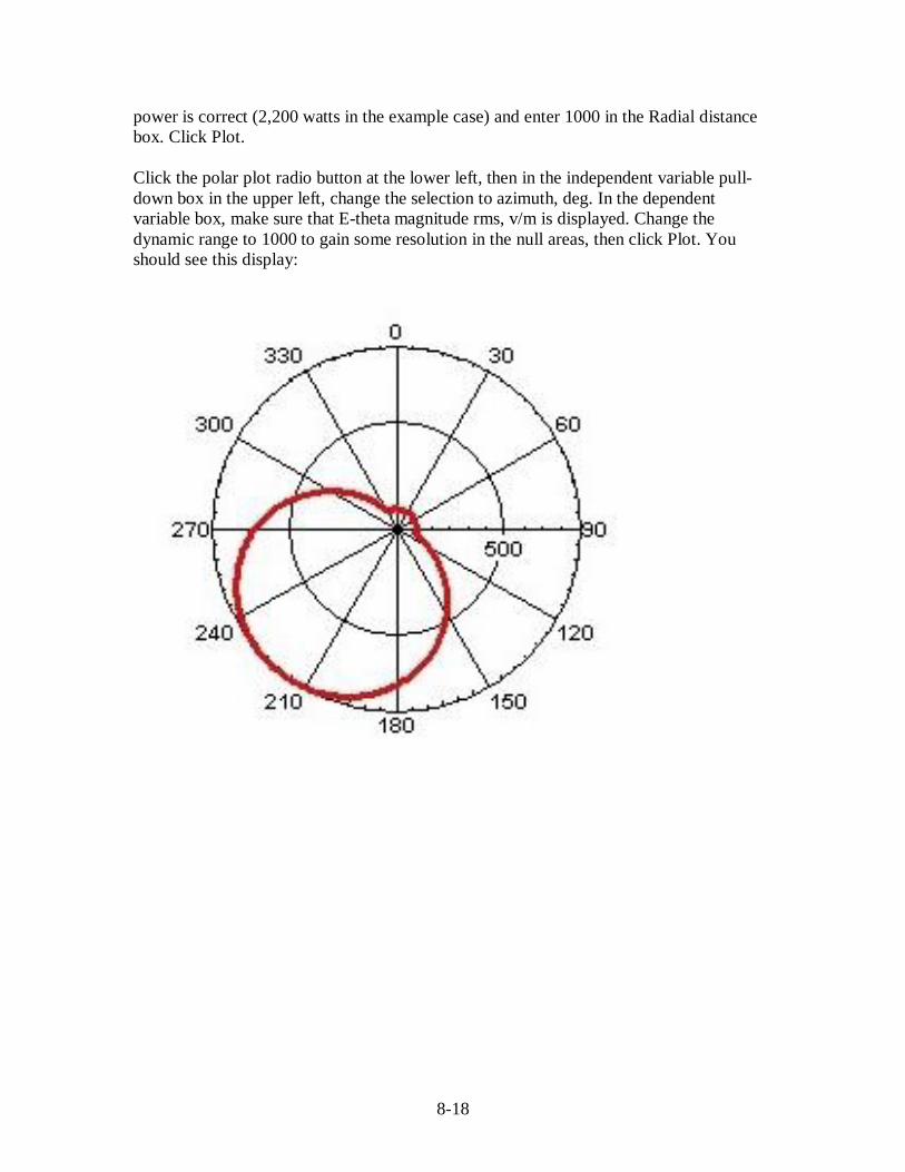
8-18

power is correct (2,200 watts in the example case) and enter 1000 in the Radial distance box. Click Plot. Click the polar plot radio button at the lower left, then in the independent variable pull-down box in the upper left, change the selection to azimuth, deg. In the dependent variable box, make sure that E-theta magnitude rms, v/m is displayed. Change the dynamic range to 1000 to gain some resolution in the null areas, then click Plot. You should see this display:

9-1

Chapter 9 : A Step-by-Step Moment Method Modeling Example (ACSModel)

Constructing the Model The example used in this section is, for the most part, the same as the one from the previous chapter, but ACSModel is used instead of MBPro. Getting Started With all the details of the directional array in hand, including element spacing, orientation, height, ratio, phase, tower face width, tower configuration and impedance matrix, the next step is to construct the model. Run ACSModel and click File | New. You will be prompted for a callsign, a description and a comment. Enter any pertinent informational data. The information entered here will be printed on each page of the output. For our example, enter: Callsign: KLVZ Description: 3-Tower Daytime Array Comment: Tower 2 driven, all others floated This information is printed on the output, so including pertinent information in the description and comment fields will help you keep track of what each model run represents. This is important when you find stacks of paper being produced, as is common in a modeling project. If you want to change the callsign, description or comment, click Problem Definition | Description (or type ctrl-d). ACSModel, which was written specifically for AM broadcast, assumes perfect ground and a ground model environment. Next, click Problem Definition | Frequency (or click ctrl-f). Set the units to kHz, set the initial frequency to 810, then click OK. Wires With the preliminaries out of the way, now it’s time to construct the actual model. Click Problem Definition | Wires (or click ctrl-w). Our tower geometry is as follows: Twr. Spacing Orientation Height 1 75.9 220 77 2 0 0 77 3 75.9 40 77

9-2

First select the Geographic coordinate system and 3 wires. In the wire 1 End One Spacing box, enter 75.9; in the orientation box, enter 220; in the Z box, enter zero. Now in the wire 1 End Two Spacing box, enter 75.9; in the orientation box, enter 220; in the Z box, enter zero. In the Radius box, enter 0.2911 (in this example, the tower has a 24-inch face, or 0.6097 meters – 3 x 0.6097 / 2 x π = 0.2911 meters effective radius). Enter 20 as the number of segments. This is a convenient number that exceeds the FCC minimum and will provide for good model performance. This establishes the wire representing tower 1. Continue by adding the bottom and top geographic coordinates for towers 2 3. Your screen should look like this:

Click OK to save the wires. It’s a good idea to save your work, so click File | Save (or click ctrl-s) and enter KLVZ-2 as the filename, navigate to the desired folder and click Save. Calibrate the Model The next step involves either floating or shorting two of the towers and driving the other to get a look at the impedance compared with the base impedance matrix for that same condition. In this case, because the towers are electrically short, the matrix was measured with the towers floated (open), so we will need to insert an open circuit at the base of two of the towers at a time. In MININEC, wires with one end at a Z value of 0 are presumed to be connected to ground (shorted), so we have to do something to lift that ground. We do this with a lumped load.

9-3

Click Problem Definition | Loads (or type ctrl-l). Remember that we are using 20 segments per tower, so pulse 1 (with a Z axis value of 0) is the base of tower 1, pulse 21 is the base of tower 2 and pulse 41 is the base of tower 3. We want to place an open circuit at the bases of towers 1 and 3, the end towers. The easiest way to do this is to enter a very high capacitive reactance at the nodes for the bases of those towers. In the Load box, select 2 for the number of loads. For the Load 1 Pulse, enter 1 for the base of tower 1. In the Resistance box, enter 0. In the Reactance box, enter -10000. This value is not critical. It needs to be a high enough reactance that no significant amount of current will flow through it at the operating frequency. Repeat this for Load 2 at node 41 for the base of tower 3. Your screen should look like this:

Click Ok to close the screen. Save your work. Now we need to drive tower 2 with a voltage source. Click Problem Definition | Sources (or type ctrl-v). The program defaults with a source at node 1. Type 21 in the Source current node box. The Sector box should default to 1. In the Magnitude box, type 1. This is not critical; any convenient value will work. The Phase box should default to zero. Click Modify. Your screen should look like this:

9-4

Click OK to close the screen. Now we’re ready for our first model run. Click Run | Run Model (or press F5). The model will run and a WordPad window will open displaying the output file. The numbers we care about are the resistance and reactance displayed under Source Data. Scroll down to find this data:

The measured tower 2 base impedance with towers 1 and 3 floated measured 28.5 +j8.5. Our first try model run, using the physical height of the tower and nominal radius, produced an impedance of 24.316 –j48.793. This is outside the FCC-specified allowance of ±2 ohms and ± 4%. We need to adjust our model. RF traveling in a steel tower moves slower than the speed of light because of all the cross-members and because of the loading effect of the guy insulators. So we can with some assurance assume the tower is electrically longer than its 77-degree physical length. Let’s assume a velocity factor of 0.9448 and rerun the model. (This value was arrived at after several iterations. Finding the right number is a sometimes lengthy trial and error process. The intermediate steps are omitted here in the interest of brevity.) Close the WordPad window, then click ctrl-w to look at the wires again. Modify each tower’s top coordinates to have a Z of 81.5 degrees (77 / 0.9448), then click Ok. 81.5 degrees is within the 75%-125% of physical height limit. Press F5 to run the model.

Twr. Meas. Baze Z, Towers Open 1 29.0 +j7.0 2 28.5 +j8.5 3 29.0 +j7.0

9-5

When the WordPad window comes up, again scroll down to Source Data to see the calculated impedance at the base of tower 2 with towers 1 and 3 floated.

Note that the impedance is now shown as 28.8 –j25.4. The resistance is within the ±2-ohm/±4% window. In fact, it’s very close to the matrix value of 28.5. But the reactance is off. Remember that the FCC rules allow a series inductance of up to10 uH. If we assume a series reactance of the opposite of +j8.5+-j25.4 (+j33.9), the model output impedance for tower 2 driven with towers 1 and 3 floated becomes 28.8 +j8.5, very close to the measured value. 33.9 / 2πF = 6.7 uH, within the allowable 10 uH limit. Next, we need to drive tower 1 and float towers 2 and 3. Type ctrl-l to bring up the Loads window. Click in the Pulse box for load 1, change it to 21 and click OK. That action got rid of the open at the base of tower 1 and moved it to the base of tower 2. Now we need to move the voltage source to the base of tower 1. Click ctrl-v to bring up the Sources window. In the Pulse window for the source at pulse 21, type 1 and click OK. This moved the source to the base of tower 1, so now we have towers 2 and 3 floated with tower 1 driven. Click ctrl-d and change the description and comment to “Tower 1 driven, all others floated.” Click ctrl-s to save and change the file name to KLVZ-1. Now we’ll run the model again. Press F5. When the WordPad window comes up, scroll down to the Source Data.

Note that the impedance from the model run is shown to be 29.5 –j24.4. The matrix impedance for tower 1 with tower 2 and 3 open measured 29.0 +j7.0, so this value of R is within the ±2 ohm/±4% window. If we add a series reactance of +j31.4, the reactance component becomes +j7.0, right on the nose. Again +j31.4 corresponds to an inductance value of less than the 10 uH FCC maximum, so we’re good. Close the WordPad window. Now we repeat the exercise by moving the pulses of the loads at the bases of towers 2 (pulse 21) and 3 (pulse 41) to the bases of towers 1 (pulse 1) and 2 (pulse 21). Then move the voltage source from pulse 1 to pulse 41, change the comment to “Tower 3 driven, all others floated and save as KLVZ-3. Run the model (F5). When the WordPad window opens, scroll down to Source Data:

9-6

The impedance is shown to be 29.5 –j24.4. The matrix Z of tower 3 driven with towers 1 and 2 open measured 29.0 +j7.0. The predicted R is within the ±2-ohm/±4% window, so it’s fine. If we use a series impedance of +j31.4, we get an X of +j7.0, right on the money. We can now consider our model to be calibrated. In some cases, it could be that once we get the first tower calibrated to the model and run the second tower with the others floated or shorted, the R is outside the ± 2-ohm/±4% window. It may then be necessary to adjust the height of the driven tower a bit to bring the R within the window. Once that is done, the bad news is that you get to re-run the previous tower again with the changed height on the second tower. That tower may now need a tweak as well. Then, if the first tower is changed, the second tower must be re-run and perhaps adjusted again. The process repeats with all the towers in the array until the full matrix is matched. This can be a time-consuming process, so be patient. An experienced modeler quickly gains a “feel” for what effect each parameter has, speeding the iteration process considerably. Modeling the Directional Pattern Once the model has been calibrated, we can move on to the next step: determining the source voltages and phases that will produce the proper fields in the individual radiators. In ACSModel, this is done internally when you enter the theoretical directional antenna parameters. Start by removing the loads producing the open circuits at the tower bases. Type ctrl-l, set the number of loads to zero and click OK. Next, go to the description (ctrl-d) and change the comment to “Directional Day” and click OK. Save the file as KLVZ-D. Now click Problem Definition | Directional Parameters (or type ctrl-b). Set the number of towers to 3 and enter the power as 2,200 watts. Next, enter the field ratios and phases for the array. Our pattern’s theoretical parameters look like this: Twr. Ratio Phase 1 0.525 -127.5 2 1.000 0 3 0.510 +124.5

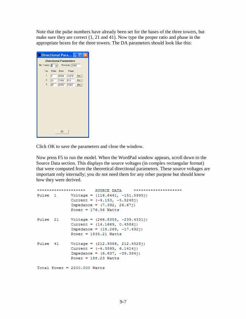
9-7

Note that the pulse numbers have already been set for the bases of the three towers, but make sure they are correct (1, 21 and 41). Now type the proper ratio and phase in the appropriate boxes for the three towers. The DA parameters should look like this:

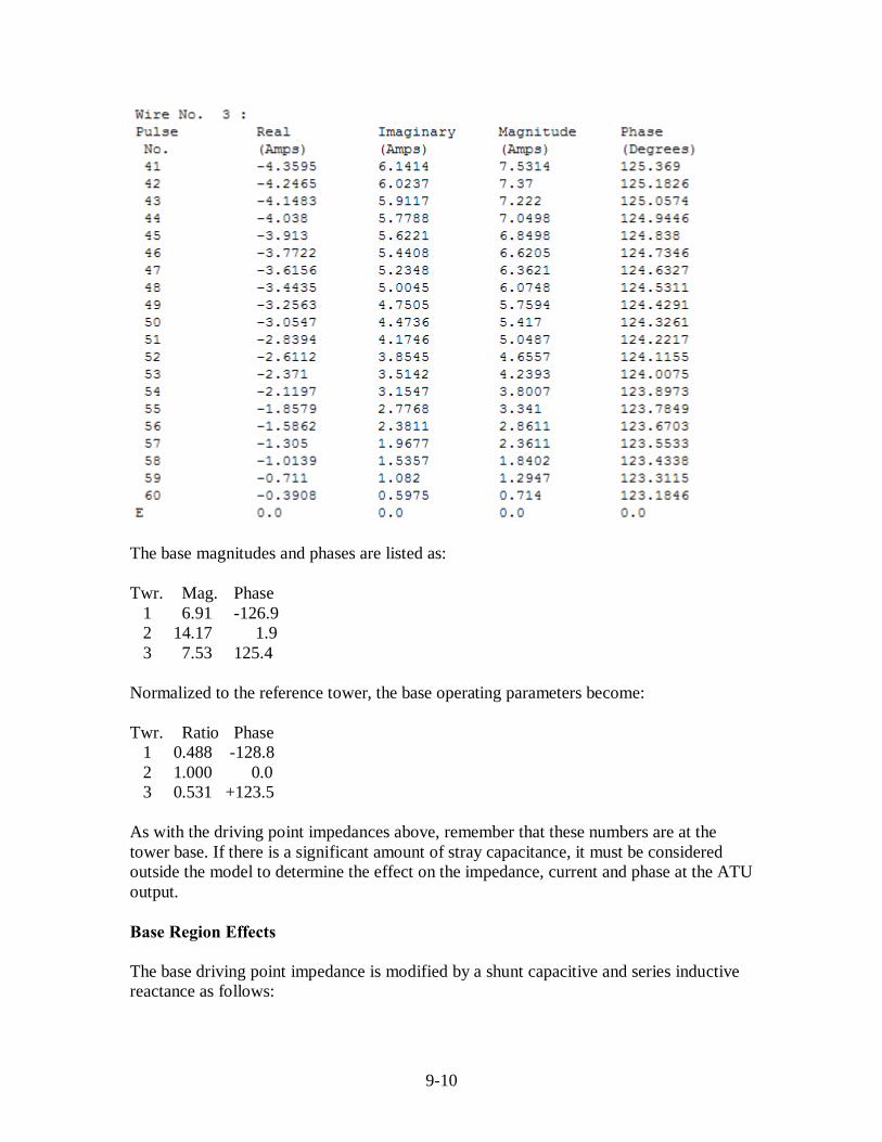
Click OK to save the parameters and close the window. Now press F5 to run the model. When the WordPad window appears, scroll down to the Source Data section. This displays the source voltages (in complex rectangular format) that were computed from the theoretical directional parameters. These source voltages are important only internally; you do not need them for any other purpose but should know how they were derived.

9-8

There is, however, information in this section that you will need. Print this page. The impedances shown, once compensated to include the series inductance values that we determined for each tower in the calibration process, will become the driving point impedances for the towers. Keep in mind here that these numbers are for the tower bases. If there are significant amounts of stray capacitance, that must be considered and factored into the driving point impedance seen at the output of the antenna tuning units. More on that later. Close the WordPad window. Now click Run | Moments (or type ctrl-m). A WordPad window will open displaying the current moments for the array. If desired, divide the current magnitude value for the two end towers by that for the reference tower to confirm that the field ratios are correct. Check the phases to make sure they are correct as well.

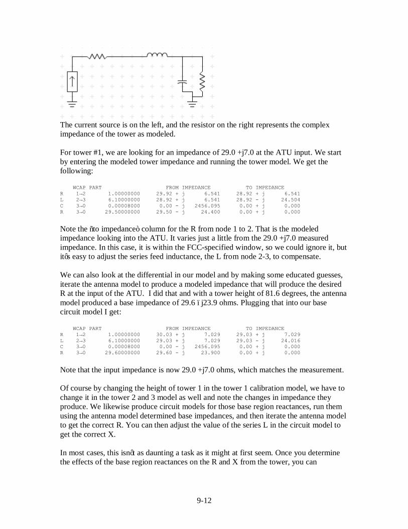
Close the WordPad window. Next, press F5 again to run the model. When the WordPad window opens, scroll down to the on the Current Data section. You should see something like the listing below. Note the magnitude and phase at the base node of each tower (1, 21 and 41). These, normalized to the values for tower 2 (reference tower), become the tower base operating parameters for the array if you are employing base sampling. ACSModel calculates and prints the base operating parameters for you, so there’s no need to do the math.

9-9

9-10

The base magnitudes and phases are listed as: Twr. Mag. Phase 1 6.91 -126.9 2 14.17 1.9 3 7.53 125.4 Normalized to the reference tower, the base operating parameters become: Twr. Ratio Phase 1 0.488 -128.8 2 1.000 0.0 3 0.531 +123.5 As with the driving point impedances above, remember that these numbers are at the tower base. If there is a significant amount of stray capacitance, it must be considered outside the model to determine the effect on the impedance, current and phase at the ATU output. Base Region Effects The base driving point impedance is modified by a shunt capacitive and series inductive reactance as follows:

9-11

RA = RBXS2/(RB

2+(XB+XS)2) XA = +jXS(RB

2+XB2+XBXS)/(RB

2+(XB+XS)2)+jXL Where: ZBASE = RB +jXB ZATU = RA +jXA XS = Shunt reactance XL = Inductive series reactance The ATU output current and phase are modified by a shunt capacitive reactance as follows: IATU Magnitude = ((1 + XB/XS)2 + (RB/XS)2)1/2 IATU Angle = arctan(-RB/XS)/(1+XB/XS) Where: IATU = ATU output current for unity base current with no phase shift ZBASE = RB +jXB XS = Shunt Reactance While you can calculate the offsets in the ATU output currents and phases using these formulas, it is much more elegant to do so using a nodal analysis program such as WCAP, available from Westberg Consulting (http://www.westbergconsulting.com). Let’s assume for a moment that we wish to base sample this array, and that the base impedance matrix measurements were made at the ATU outputs (as you should when base sampling). Our array employs Austin transformers and no lighting chokes, so we have only two base region reactances to deal with: the series feed inductance and the shunt capacitance of the base insulator. The series feed inductance can be all over the map up to 10 uH, so we will determine that separately. Base insulator capacitance is generally in the 50 to 100 pF range, depending on the length and diameter of the insulator. For this exercise, we will use a value of 80 pF. In WCAP Pro, we will construct a circuit model with each of these elements, and to provide ourselves with a node at which to measure the impedance looking into the network, we will employ a one-ohm resistor between the network input and the series feed inductance. The model looks like this:

9-12

The current source is on the left, and the resistor on the right represents the complex impedance of the tower as modeled. For tower #1, we are looking for an impedance of 29.0 +j7.0 at the ATU input. We start by entering the modeled tower impedance and running the tower model. We get the following: WCAP PART FROM IMPEDANCE TO IMPEDANCE R 1→2 1.00000000 29.92 + j 6.541 28.92 + j 6.541 L 2→3 6.10000000 28.92 + j 6.541 28.92 - j 24.504 C 3→0 0.00008000 0.00 - j 2456.095 0.00 + j 0.000 R 3→0 29.50000000 29.50 - j 24.400 0.00 + j 0.000 Note the “to impedance” column for the R from node 1 to 2. That is the modeled impedance looking into the ATU. It varies just a little from the 29.0 +j7.0 measured impedance. In this case, it is within the FCC-specified window, so we could ignore it, but it’s easy to adjust the series feed inductance, the L from node 2-3, to compensate. We can also look at the differential in our model and by making some educated guesses, iterate the antenna model to produce a modeled impedance that will produce the desired R at the input of the ATU. I did that and with a tower height of 81.6 degrees, the antenna model produced a base impedance of 29.6 –j23.9 ohms. Plugging that into our base circuit model I get: WCAP PART FROM IMPEDANCE TO IMPEDANCE R 1→2 1.00000000 30.03 + j 7.029 29.03 + j 7.029 L 2→3 6.10000000 29.03 + j 7.029 29.03 - j 24.016 C 3→0 0.00008000 0.00 - j 2456.095 0.00 + j 0.000 R 3→0 29.60000000 29.60 - j 23.900 0.00 + j 0.000 Note that the input impedance is now 29.0 +j7.0 ohms, which matches the measurement. Of course by changing the height of tower 1 in the tower 1 calibration model, we have to change it in the tower 2 and 3 model as well and note the changes in impedance they produce. We likewise produce circuit models for those base region reactances, run them using the antenna model determined base impedances, and then iterate the antenna model to get the correct R. You can then adjust the value of the series L in the circuit model to get the correct X. In most cases, this isn’t as daunting a task as it might at first seem. Once you determine the effects of the base region reactances on the R and X from the tower, you can

9-13

determine a new target impedance (with the R component being most important, since you can adjust the X with the series inductor) and then recalibrate the model. At the end of this process, you will have a calibrated antenna model for each tower and a calibrated circuit model for each tower. Directional Parameter Offsets The next step is to run the recalibrated antenna model in the directional mode, then plug the antenna model determined driving point impedances into the circuit models. In our example, we get the following impedances from the DA model: ******************** SOURCE DATA ******************** Pulse 1 Voltage = (120.4038, -154.3533j) Current = (-4.1438, -5.5128j) Impedance = (7.401, 27.403j) Power = 176.0 Watts Pulse 21 Voltage = (267.4752, -218.4383j) Current = (14.0962, 0.4609j) Impedance = (18.449, -16.099j) Power = 1834.86 Watts Pulse 41 Voltage = (209.4141, 210.3891j) Current = (-4.3525, 6.1304j) Impedance = (6.692, -38.911j) Power = 189.15 Watts Total Power = 2200.000 Watts So in the tower 1 circuit model, we set the load resistor to 7.401 +j27.403. I then set the input current to 100 amps with a phase of zero. I do this to get some resolution in the model. Running the circuit model, we see the following output: WCAP PART BRANCH VOLTAGE BRANCH CURRENT R 1→2 1.00000000 100.00 ∡ 0.000° V 100.00 ∡ 0.000° A L 2→3 6.10000000 3104.52 ∡ 90.000° V 100.00 ∡ 0.000° A C 3→0 0.00008000 2870.50 ∡ 74.712° V 1.17 ∡ 164.712° A R 3→0 7.40100000 2870.50 ∡ 74.712° V 101.13 ∡ -0.175° A The figures of interest are the branch current magnitude and phase for the input R (nodes 1-2) and the output R (nodes 3-0). The differential shows us the shift in current magnitude and phase through the base region reactances. In this case, we note that the output current is 1.13% higher than the input current, and the phase is retarded by 0.175 degrees. So to compensate for that, we reduce the current at the input by 1.13% and advance the phase by 0.175 degrees. The directional antenna model shows the following for pulse 1 (the base) of tower 1: ******************** CURRENT DATA ******************** Wire No. 1 : Pulse Real Imaginary Magnitude Phase No. (Amps) (Amps) (Amps) (Degrees) 1 -4.1438 -5.5128 6.8966 -126.931

9-14

So we increase the 6.8966 amps by 1.13% (6.986A) and advance the -126.931 degrees by 0.175 degrees (-126.756) and plug those values into the current source of our directional circuit model for tower 1. That yields: WCAP PART BRANCH VOLTAGE BRANCH CURRENT R 1→2 1.00000000 6.82 ∡ -126.756° V 6.82 ∡ -126.756° A L 2→3 6.10000000 211.73 ∡ -36.756° V 6.82 ∡ -126.756° A C 3→0 0.00008000 195.77 ∡ -52.044° V 0.08 ∡ 37.956° A R 3→0 7.40100000 195.77 ∡ -52.044° V 6.90 ∡ -126.931° A Note that the output current of the circuit model, which represents the tower base, now matches the antenna model determined current at the tower base. We do the same thing for the other two towers: plug the DA model driving point impedances into the circuit models for the respective towers, determine the current magnitude and phase offsets, then adjust the antenna model determined base current magnitude and phase by those offsets and plug them into the circuit model. The base-sampled operating parameters of the array are then determined from the input current magnitudes and phases of the circuit models. In the case of our example, the DA base circuit model outputs look like this: Tower 1 WCAP PART BRANCH VOLTAGE BRANCH CURRENT R 1→2 1.00000000 6.82 ∡ -126.756° V 6.82 ∡ -126.756° A L 2→3 6.10000000 211.73 ∡ -36.756° V 6.82 ∡ -126.756° A C 3→0 0.00008000 195.77 ∡ -52.044° V 0.08 ∡ 37.956° A R 3→0 7.40100000 195.77 ∡ -52.044° V 6.90 ∡ -126.931° A Tower 2 WCAP PART BRANCH VOLTAGE BRANCH CURRENT R 1→2 1.00000000 14.20 ∡ 2.299° V 14.20 ∡ 2.299° A L 2→3 6.43000000 464.53 ∡ 92.299° V 14.20 ∡ 2.299° A C 3→0 0.00008000 344.79 ∡ -39.314° V 0.14 ∡ 50.686° A R 3→0 18.40000000 344.79 ∡ -39.314° V 14.10 ∡ 1.872° A Tower 3 WCAP PART BRANCH VOLTAGE BRANCH CURRENT R 1→2 1.00000000 7.63 ∡ 125.528° V 7.63 ∡ 125.528° A L 2→3 6.10000000 236.91 ∡ -144.472° V 7.63 ∡ 125.528° A C 3→0 0.00008000 296.52 ∡ 45.147° V 0.12 ∡ 135.147° A R 3→0 6.70000000 296.52 ∡ 45.147° V 7.51 ∡ 125.374° A

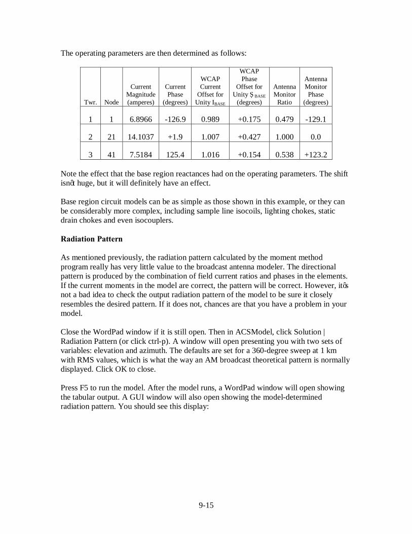
9-15

The operating parameters are then determined as follows:

Twr.

Node

Current Magnitude (amperes)

Current Phase

(degrees)

WCAP Current

Offset for Unity IBASE

WCAP Phase

Offset for Unity ǾBASE

(degrees)

Antenna Monitor

Ratio

Antenna Monitor Phase

(degrees)

1 1 6.8966 -126.9 0.989 +0.175 0.479 -129.1

2 21 14.1037 +1.9 1.007 +0.427 1.000 0.0

3 41 7.5184 125.4 1.016 +0.154 0.538 +123.2 Note the effect that the base region reactances had on the operating parameters. The shift isn’t huge, but it will definitely have an effect. Base region circuit models can be as simple as those shown in this example, or they can be considerably more complex, including sample line isocoils, lighting chokes, static drain chokes and even isocouplers. Radiation Pattern As mentioned previously, the radiation pattern calculated by the moment method program really has very little value to the broadcast antenna modeler. The directional pattern is produced by the combination of field current ratios and phases in the elements. If the current moments in the model are correct, the pattern will be correct. However, it’s not a bad idea to check the output radiation pattern of the model to be sure it closely resembles the desired pattern. If it does not, chances are that you have a problem in your model. Close the WordPad window if it is still open. Then in ACSModel, click Solution | Radiation Pattern (or click ctrl-p). A window will open presenting you with two sets of variables: elevation and azimuth. The defaults are set for a 360-degree sweep at 1 km with RMS values, which is what the way an AM broadcast theoretical pattern is normally displayed. Click OK to close. Press F5 to run the model. After the model runs, a WordPad window will open showing the tabular output. A GUI window will also open showing the model-determined radiation pattern. You should see this display:

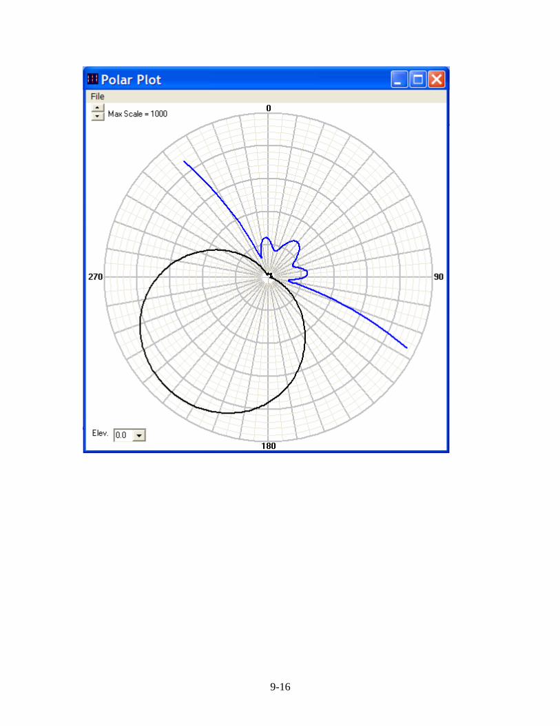
9-16

10-1

Chapter 10 : Tower-Mounted Loop Sampling The example thus far has dealt with base sampling, but what if tower-mounted loop sampling is desired? The procedure is a little different. To determine the sample loop location, we must find the elevation where the current in the tower would be at a minimum if the tower were detuned. The procedure to do this is to drive one tower only. We’ll show you here how to do this in both MBPro and ACSModel. MBPro Example Click ctrl-b to go to the array synthesis window. 3 should be displayed in the box for the number of towers. Click Ok to display the tower parameter input screen. Click on the line for tower 1 (node 1) and change the Field magnitude ratio to 0 and click Modify. Click on the line for tower 3 (node 41) and change the Field magnitude ratio to 0 and click Modify. This sets the array synthesis to drive tower 2 and not towers 1 and 3. Click Ok to close. Press F5, select “Currents admittance coupling...” and click Ok. Save the file with a new filename (use detune in the filename so you will know what the file is). When the Display options window is displayed, click Array synthesis and Text. A WordPad window will open showing the array synthesis and the sources to drive the array. Check to make sure that the tower 1 and 3 ratios are set to zero and tower 2 is set to 1. Close the WordPad window. Press F5, select “Currents admittance coupling...” and click Ok. When the Display options window appears, click impedance and Text. A WordPad window will open showing the following:

To detune an array element, the tower must be terminated in the opposite of its zero-field impedance. In this case, towers 1 and 3 would need to be terminated in 25 +j638 ohms. Simply terminating them in +j638 will generally detune the tower, but this reactance will

10-2

have to be fine-tuned to minimize the reradiated field. To do this in the model, we create a new model of just one tower. Click File | New and select Broadcast Antenna. For the description, enter “81.5-degree tower detune” or some other meaningful descriptor. Type ctrl-f and set the frequency to 810 kHz. Type ctrl-n and make sure Dimensions is set to degrees, Coordinates is set to geographic and Environment is set to perfect ground. Create a node at 0, 0, 0 and another at 0, 0, 81.5, then click Ok to close the window. Type ctrl-w and create a wire from node 1 to node 2. Set the radius to 0.2188 and set segments to 20. Close the window with Ok. Now we’ll do something new. Click Problem definition | Electrical | Plane wave source (or press F11). With this, we will simulate a plane wave arriving at the tower from a particular azimuth and elevation to see what current it induces into the tower. This will allow us to determine what it will take to detune the tower and then it will tell us the elevation where the current in the tower would be at a minimum if the tower were detuned. Enter a zenith initial value of 90, set the increment to zero and the number of angles to 1. Next, enter the azimuth initial value of 0, set the increment to zero and the number of angles to 1. The zenith value is critical here, but the azimuth does not matter on this non-directional radiator. Set the polarization angle to zero and the magnitude to 10 volts (not critical, but using 10 volts here will give us some resolution (and 10 volts is not an unreasonable value for an incident electric field on a floated tower in a directional array). Click Ok to close the window. Next, we need to enter a terminating load at the base of the tower. Type ctrl-l and create a zero ohm resistance +j638 ohm reactance load at node 1. Click Ok to close the window. Now type ctrl-p to bring up the radiation pattern calculation window. Make sure the coordinate system is set to geographic, then set the zenith initial angle to zero, the increment to zero and the number of angles to 1. Set the azimuth initial angle to zero, the increment to zero and the number of angles to 1. We could do a 36, 72 or 360 radial sweep, but on this single, non-directional tower all the values will be the same, so one radial will be adequate. Click Ok to close the window. Now we’re ready to run the model. Press F5. Check Currents and Radiation pattern and click Ok. Save the file with a new name that indicates that this is a single detuned tower model. On the Display options window, click current and Text. A WordPad window should open and display something like this:

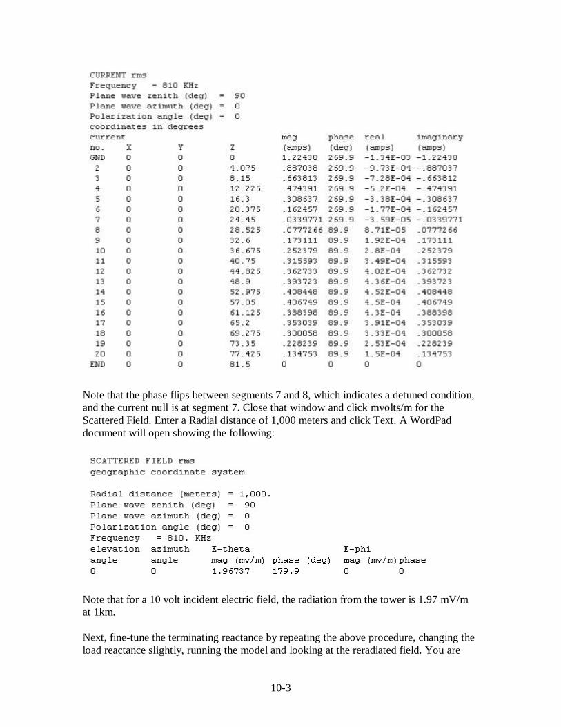
10-3

Note that the phase flips between segments 7 and 8, which indicates a detuned condition, and the current null is at segment 7. Close that window and click mvolts/m for the Scattered Field. Enter a Radial distance of 1,000 meters and click Text. A WordPad document will open showing the following:

Note that for a 10 volt incident electric field, the radiation from the tower is 1.97 mV/m at 1km. Next, fine-tune the terminating reactance by repeating the above procedure, changing the load reactance slightly, running the model and looking at the reradiated field. You are

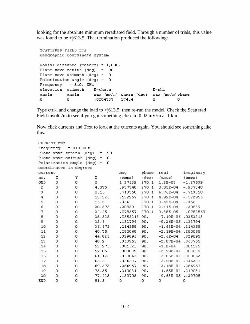
10-4

looking for the absolute minimum reradiated field. Through a number of trials, this value was found to be +j613.5. That termination produced the following:

Type ctrl-l and change the load to +j613.5, then re-run the model. Check the Scattered Field mvolts/m to see if you got something close to 0.02 mV/m at 1 km. Now click currents and Text to look at the currents again. You should see something like this:

10-5

The correct operating parameters for this array would be the currents and phases for segment 8 of each tower. Note that the phase of the current on the tower flips between segments 7 and 8, and the segment with the minimum current is number 8. We have thus identified the elevation where the current in the tower would be at a minimum if the tower were detuned. That is the elevation where the sample loops on all the towers of that height in the array would be located. The FCC rules require that if the effective height of the array element has been adjusted to match the Z matrix, the loops must be mounted at the same percentage height as indicated in the model. In this example, our towers are 77 degrees physical height and the model effective height is 81.5 degrees. Segment 8 on the 81.5-degree radiator is centered at 28.525 degrees above the base, so the loop height on the actual tower is computed as: 28.525 / 81.5 x 77 = 26.95 degrees, or 90.84 feet above the base of the tower. What parameters would we look for, then, on our antenna monitor with the loops mounted at this height? Look at the currents again on pages 7-14 through 7-16. Note the segment 8 tower 2 current (node 28) is 8.44519 amps at 360 degrees. That corresponds to a ratio of 1.000 and a phase of 0 for the reference tower. Note the segment 8 tower 1 current (node 8) is 4.44903 amps at 232.4 degrees. That represents a ratio of 0.527 and a phase of -127.6 degrees. Note the segment 8 tower 3 current (node 48) is 4.29942 amps at 124.5 degrees. That represents a ratio of 0.509 and a phase of +124.5 degrees. The loop-sampled array parameters would then be: Twr. Ratio Phase 1 0.527 -127.6 2 1.000 0.0 3 0.509 +124.5 ACSModel Example The process is considerable simpler in ACSModel, owing to the fact that ACSModel was written specifically for AM broadcast work. First, set up a new model (ctrl-n) with a single towers of the same height (81.6 deg.), radius (0.2911 meters) and number of segments (20) as used in the calibrated model. Now click Run | Detune. The model will run several times, iterating internally to find the reactance necessary to detune the tower. A window will open showing that value of reactance.

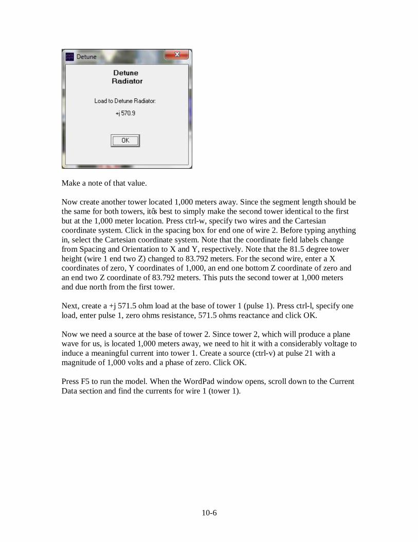
10-6

Make a note of that value. Now create another tower located 1,000 meters away. Since the segment length should be the same for both towers, it’s best to simply make the second tower identical to the first but at the 1,000 meter location. Press ctrl-w, specify two wires and the Cartesian coordinate system. Click in the spacing box for end one of wire 2. Before typing anything in, select the Cartesian coordinate system. Note that the coordinate field labels change from Spacing and Orientation to X and Y, respectively. Note that the 81.5 degree tower height (wire 1 end two Z) changed to 83.792 meters. For the second wire, enter a X coordinates of zero, Y coordinates of 1,000, an end one bottom Z coordinate of zero and an end two Z coordinate of 83.792 meters. This puts the second tower at 1,000 meters and due north from the first tower. Next, create a +j 571.5 ohm load at the base of tower 1 (pulse 1). Press ctrl-l, specify one load, enter pulse 1, zero ohms resistance, 571.5 ohms reactance and click OK. Now we need a source at the base of tower 2. Since tower 2, which will produce a plane wave for us, is located 1,000 meters away, we need to hit it with a considerably voltage to induce a meaningful current into tower 1. Create a source (ctrl-v) at pulse 21 with a magnitude of 1,000 volts and a phase of zero. Click OK. Press F5 to run the model. When the WordPad window opens, scroll down to the Current Data section and find the currents for wire 1 (tower 1).

10-7

Note that at pulse 8, the current magnitude is at a minimum (and the phase of the current flips positive). Pulse 8, then, is the location at which the sample loop must be positioned on this particular tower. If we scroll up to the Antenna Geometry section for wire 1, we can see that pulse 8 is 29.3272 meters above the base. In this example, all three towers calibrate at the same height, so we need do this only once. If, however, we had towers of different calibrated heights, we would have to repeat this entire process for each tower, thus determining the detuning reactance and sample loop elevation for each tower. If the differences in tower heights are less than half a segment, you can get away with going through the process just once, for the tower closest to the median height of the array. The same procedure as discussed in the MBPro section above applies here in determining the physical elevation of the sample loops and the loop operating parameters.

11-1

Chapter 11 : Sampling Systems for Modeled DA Proofs The Traditional Sample System A traditional directional sample system consists of either tower-mounted pickup loops or current transformers installed at the output of the antenna tuning units (ATUs), an antenna monitor, and a transmission line connecting each pickup device to the antenna monitor. In most cases, the sample transmission lines are of equal length, and in many cases, the sample lines are phase-stabilized, which means that they have been temperature cycled over a specified range in an oven of sorts at the factory. Over the years, those constructing and adjusting AM directional arrays have made a good effort to insure the accuracy of the sample system, at least to the degree possible with test equipment on hand. Sample loops are constructed as close to identically as possible, current transformers are certified by the manufacturer to be accurate to within 2% for magnitude and to within 3 degrees for phase, and sample lines are carefully cut to have equal electrical length. The Modeled Array Sample System While the sample system performs the same job in the moment method modeling world, its accuracy and stability take on new import. In a traditional measurement-verified directional antenna system, the sample system’s primary job is to monitor the stability of the operating parameters. In a model-proofed array, it is used to monitor stability but also serves as the means by which the array is set up. As such, its accuracy, stability and linearity are critical. A sample system must be able to measure voltage or current as it is modeled for each directional antenna element. Current samples can be, as noted above, tower-mounted loops or current transformers at the ATU output. Kintronic Laboratories is now making a voltage sampler in a weatherproof cabinet that can be connected in shunt with the ATU output. The sample produced by these devices must exclude influences that cannot be modeled accurately. Some examples are towers with non-radiating sampled currents that cannot be modeled, such as skirt-fed towers (folded unipoles) and slant-wire fed towers. Base Sampling A tower that is base sampled should have its current transformers located at the same point where the base impedance matrix measurements were made. As such, it is important in base-sampled towers to measure the matrix at the ATU outputs. A tower-mounted sample loop cannot be used to base sample a tower.

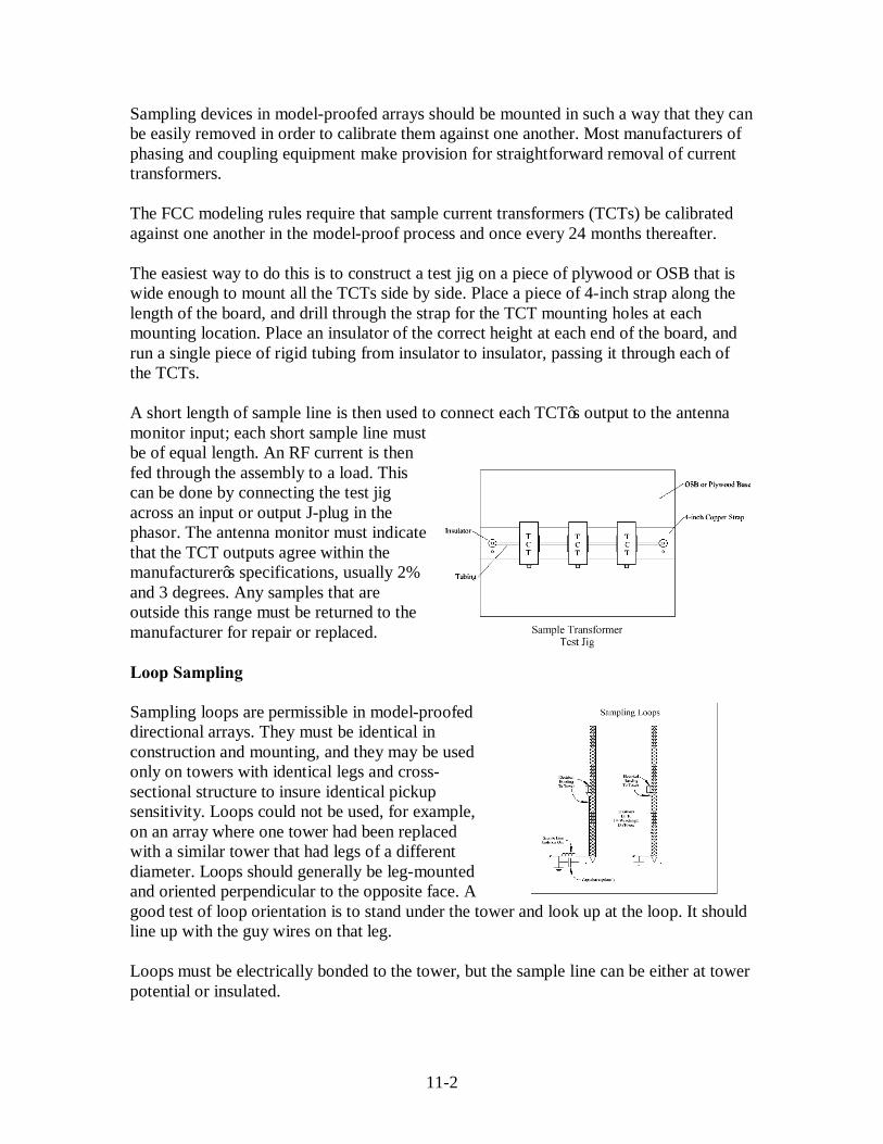
11-2

Sampling devices in model-proofed arrays should be mounted in such a way that they can be easily removed in order to calibrate them against one another. Most manufacturers of phasing and coupling equipment make provision for straightforward removal of current transformers. The FCC modeling rules require that sample current transformers (TCTs) be calibrated against one another in the model-proof process and once every 24 months thereafter. The easiest way to do this is to construct a test jig on a piece of plywood or OSB that is wide enough to mount all the TCTs side by side. Place a piece of 4-inch strap along the length of the board, and drill through the strap for the TCT mounting holes at each mounting location. Place an insulator of the correct height at each end of the board, and run a single piece of rigid tubing from insulator to insulator, passing it through each of the TCTs. A short length of sample line is then used to connect each TCT’s output to the antenna monitor input; each short sample line must be of equal length. An RF current is then fed through the assembly to a load. This can be done by connecting the test jig across an input or output J-plug in the phasor. The antenna monitor must indicate that the TCT outputs agree within the manufacturer’s specifications, usually 2% and 3 degrees. Any samples that are outside this range must be returned to the manufacturer for repair or replaced. Loop Sampling Sampling loops are permissible in model-proofed directional arrays. They must be identical in construction and mounting, and they may be used only on towers with identical legs and cross-sectional structure to insure identical pickup sensitivity. Loops could not be used, for example, on an array where one tower had been replaced with a similar tower that had legs of a different diameter. Loops should generally be leg-mounted and oriented perpendicular to the opposite face. A good test of loop orientation is to stand under the tower and look up at the loop. It should line up with the guy wires on that leg. Loops must be electrically bonded to the tower, but the sample line can be either at tower potential or insulated.

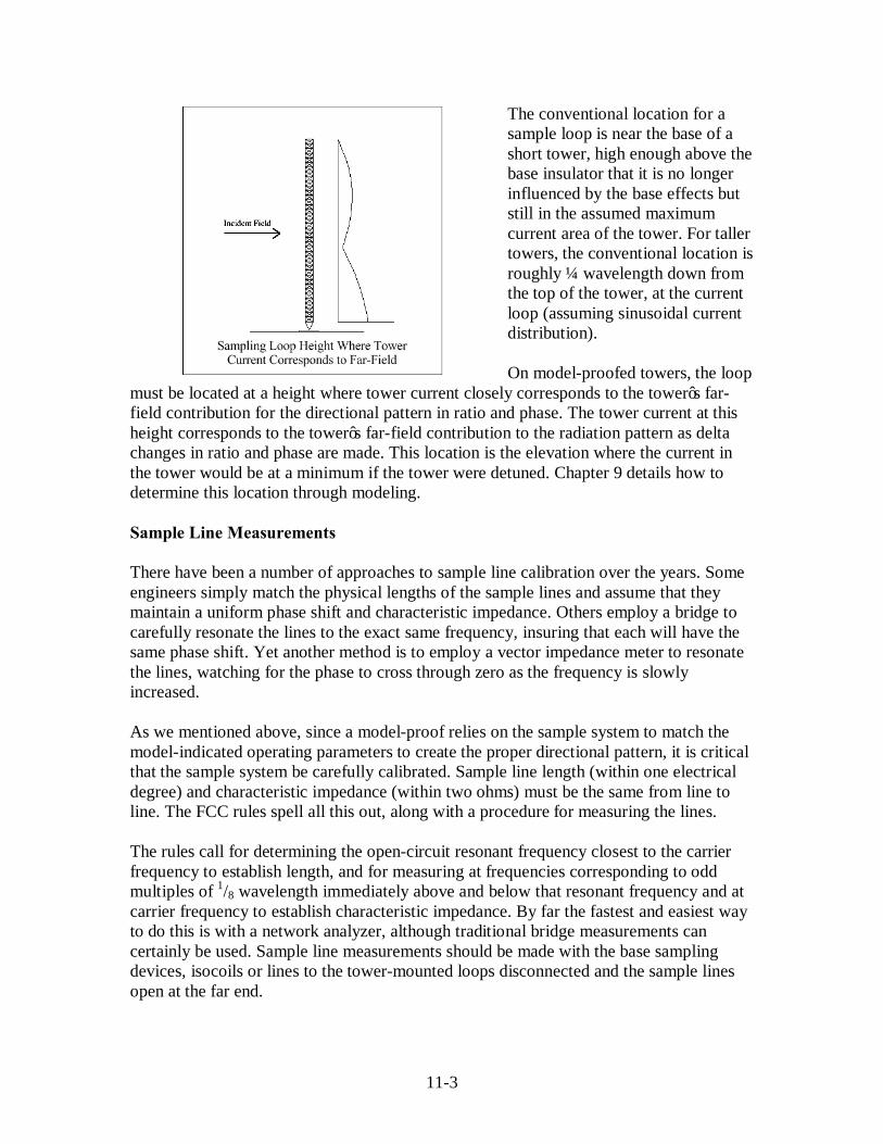
11-3

The conventional location for a sample loop is near the base of a short tower, high enough above the base insulator that it is no longer influenced by the base effects but still in the assumed maximum current area of the tower. For taller towers, the conventional location is roughly ¼ wavelength down from the top of the tower, at the current loop (assuming sinusoidal current distribution). On model-proofed towers, the loop

must be located at a height where tower current closely corresponds to the tower’s far-field contribution for the directional pattern in ratio and phase. The tower current at this height corresponds to the tower’s far-field contribution to the radiation pattern as delta changes in ratio and phase are made. This location is the elevation where the current in the tower would be at a minimum if the tower were detuned. Chapter 9 details how to determine this location through modeling. Sample Line Measurements There have been a number of approaches to sample line calibration over the years. Some engineers simply match the physical lengths of the sample lines and assume that they maintain a uniform phase shift and characteristic impedance. Others employ a bridge to carefully resonate the lines to the exact same frequency, insuring that each will have the same phase shift. Yet another method is to employ a vector impedance meter to resonate the lines, watching for the phase to cross through zero as the frequency is slowly increased. As we mentioned above, since a model-proof relies on the sample system to match the model-indicated operating parameters to create the proper directional pattern, it is critical that the sample system be carefully calibrated. Sample line length (within one electrical degree) and characteristic impedance (within two ohms) must be the same from line to line. The FCC rules spell all this out, along with a procedure for measuring the lines. The rules call for determining the open-circuit resonant frequency closest to the carrier frequency to establish length, and for measuring at frequencies corresponding to odd multiples of 1/8 wavelength immediately above and below that resonant frequency and at carrier frequency to establish characteristic impedance. By far the fastest and easiest way to do this is with a network analyzer, although traditional bridge measurements can certainly be used. Sample line measurements should be made with the base sampling devices, isocoils or lines to the tower-mounted loops disconnected and the sample lines open at the far end.

11-4

In an unterminated transmission line, impedance zeros will occur at odd multiples of 90 degrees electrical length (i.e. 90 deg., 270 deg., 450 deg., etc.) as the electrical length is varied by changing frequency. An impedance zero is where the reactance passed through zero and, for lines with loss, resistance is low. The procedure for this is to determine the multiple of 90 degrees for the zero closest to the carrier frequency, then ratio that length to the length at carrier frequency. Again, a network analyzer presents the fastest and easiest means of making all the required measurements. Start with the known physical length of the line (or if unknown, use a TDR to find the physical length).Use the equation F = 4 x 984 / L / VF to find the approximate ¼ λ frequency for that length of line, where L is the physical length of the line and VF is the assumed velocity factor as a decimal. Now disconnect the tower end of the sample line and leave it open. Set up the analyzer for a one-port (S11) measurement, Smith chart R +jX. Go through the open and short calibration procedure for your analyzer, then set up the sweep. The lower (start) frequency needs to be well below the ¼ λ frequency and the upper (stop) needs to be well above the ¾ λ frequency. If the ¼ λ frequency is below the lower frequency range of the analyzer, set the sweep to start well below the ¾ λ frequency and to end well above the 5/4 λ frequency. Connect the monitor end of the sample line to the S1 port of the analyzer. Use enough power to overcome any stray RF that might otherwise contaminate the measurement. The display should show a spiral that crosses the left side of the zero X line at least twice. Use the markers feature to determine the frequency of each left side zero crossing. The X will be zero or very close to it at this point; the R represents the resistive loss of the sample line. Because you know the quarter-wavelength multiple at each zero crossing, it’s easy to find the one closest to the carrier frequency. In the example below, the carrier frequency of the station is 670 kHz. The zero crossings (markers 1 and 2) occur at 600 kHz and 1006 kHz for the ¾ λ (270 degree) and 5/4 λ (450 degree) multiples, respectively. The 600 kHz crossing is closest to carrier frequency. From that we can determine the electrical length of the sample line in degrees: 670 / 600 x 270 = 301.5 degrees

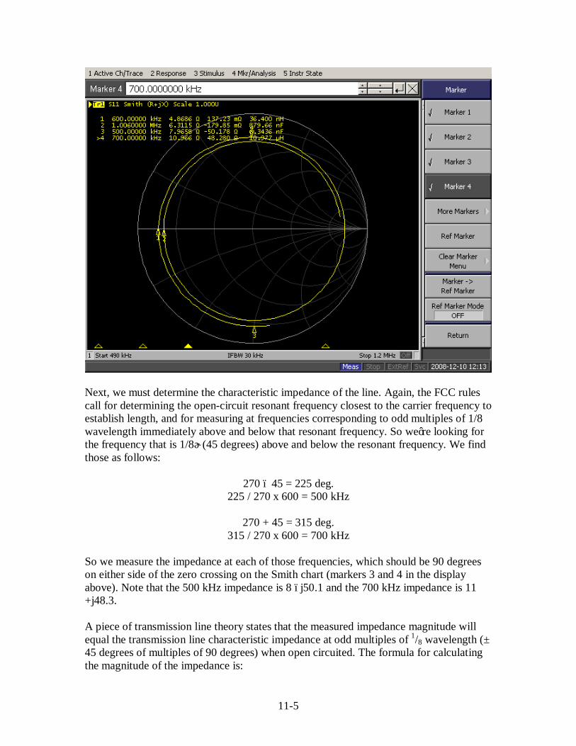
11-5

Next, we must determine the characteristic impedance of the line. Again, the FCC rules call for determining the open-circuit resonant frequency closest to the carrier frequency to establish length, and for measuring at frequencies corresponding to odd multiples of 1/8 wavelength immediately above and below that resonant frequency. So we’re looking for the frequency that is 1/8λ (45 degrees) above and below the resonant frequency. We find those as follows:

270 – 45 = 225 deg. 225 / 270 x 600 = 500 kHz

270 + 45 = 315 deg.

315 / 270 x 600 = 700 kHz So we measure the impedance at each of those frequencies, which should be 90 degrees on either side of the zero crossing on the Smith chart (markers 3 and 4 in the display above). Note that the 500 kHz impedance is 8 –j50.1 and the 700 kHz impedance is 11 +j48.3. A piece of transmission line theory states that the measured impedance magnitude will equal the transmission line characteristic impedance at odd multiples of 1/8 wavelength (± 45 degrees of multiples of 90 degrees) when open circuited. The formula for calculating the magnitude of the impedance is:

11-6

ZO = (RIN2+XIN

2)1/2 So… For the -45 degree frequency, ZO = (82+50.12) ½ = 50.7 Ohms For the +45 degree frequency, ZO = (112+48.32) ½ = 49.5 Ohms While from an engineering perspective it would be desirable to have a measured characteristic impedance that matches the output impedance of the sample device and the input impedance of the antenna monitor, the important factor from a model-proof standpoint is that the characteristic impedances of the lines are all within ±2 ohms of one another. In many sample systems, there are several segments of sample lines per tower. Systems with loops and isolation coils have separate horizontal runs, isolation coils and tower runs. The entire length can be measured as a single line or the sections may be measured separately and their lengths added together to determine the total length. Measuring Sample Lines into Sample Loops Tower-mounted sample loops present a somewhat more difficult situation than base sample current transformers. Tower-mounted loops are difficult to access, and generally speaking, once a loop connection has been made and weatherproofed, it’s best to leave it alone (we have all likely had bad experiences with tower crews opening and re-sealing a weatherproofed connection). When an array is model-proofed for the first time, it is likely that the loops will have to be relocated on the tower to place them at the proper elevation. At that time, there is a unique, one-time opportunity to measure the entire length of the open sample line for each tower, and you should take advantage of that. But once the loop is connected, it would be expensive and unwise to send a tower worker up each tower to open each connector, especially since the loop impedance (actually the impedance of the sample line terminated in the loop) must be measured anyway. Sample line measurements can be made with the loops connected. Obviously, all excitation must be removed from the array before this is done. Loops, as they are required to be identical, may be assumed to be identical terminating loads for the unmatched sample lines. As the sample lines are equal in length, measurements on different lines will confirm equal lengths and equal loop characteristics by examining the observed reflection coefficients as follows:

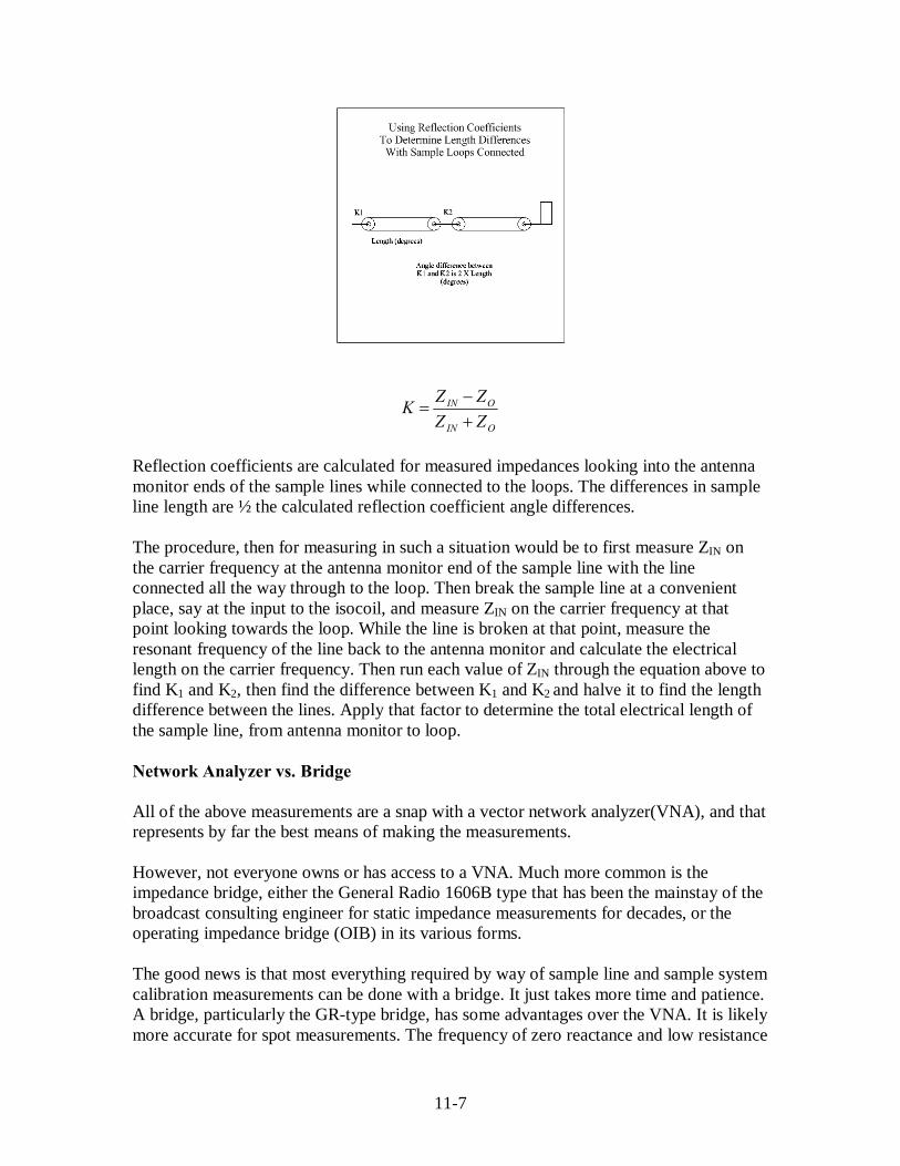
11-7

OIN

OIN

ZZZZK

+−

=

Reflection coefficients are calculated for measured impedances looking into the antenna monitor ends of the sample lines while connected to the loops. The differences in sample line length are ½ the calculated reflection coefficient angle differences. The procedure, then for measuring in such a situation would be to first measure ZIN on the carrier frequency at the antenna monitor end of the sample line with the line connected all the way through to the loop. Then break the sample line at a convenient place, say at the input to the isocoil, and measure ZIN on the carrier frequency at that point looking towards the loop. While the line is broken at that point, measure the resonant frequency of the line back to the antenna monitor and calculate the electrical length on the carrier frequency. Then run each value of ZIN through the equation above to find K1 and K2, then find the difference between K1 and K2 and halve it to find the length difference between the lines. Apply that factor to determine the total electrical length of the sample line, from antenna monitor to loop. Network Analyzer vs. Bridge All of the above measurements are a snap with a vector network analyzer(VNA), and that represents by far the best means of making the measurements. However, not everyone owns or has access to a VNA. Much more common is the impedance bridge, either the General Radio 1606B type that has been the mainstay of the broadcast consulting engineer for static impedance measurements for decades, or the operating impedance bridge (OIB) in its various forms. The good news is that most everything required by way of sample line and sample system calibration measurements can be done with a bridge. It just takes more time and patience. A bridge, particularly the GR-type bridge, has some advantages over the VNA. It is likely more accurate for spot measurements. The frequency of zero reactance and low resistance

11-8

is unmistakable with such an instrument. The bad news is that finding that frequency means constant initial balance adjustments, repeated at every new frequency. It takes a lot of iterations to nail down the resonant frequency of the line. Still, it can be done with a bridge, and that fact should encourage those who perhaps might otherwise avoid the model-proof option because they do not have access to a VNA. Another advantage of a bridge over a VNA is its ability to work in the presence of (relatively) high RF fields. Consider the case of a directional array in a large city where there are many AM signals, some of their sites quite close by (within five miles or so) and with high incident fields. Most VNA inputs have a maximum level of +20 dBm, which can easily be exceeded in such a situation – particularly when coupling to a tower-mounted sample loop. An impedance bridge, which with its accompanying detector is highly frequency selective, has no such limitation.

12-1

Chapter 12 : Analyzing Potential Reradiators Using Moment Method Modeling

Traditional Methods Over the years, we have employed a number of methods of potential reradiator analysis. Most of these have been based on a fixed amount of loss (no-loss or 50%), representing essentially worst-case conditions. These methods tended to overestimate the reradiation from a given structure. In the 9th Edition of the NAB Engineering Handbook, a formula was published that has become universally used throughout the industry. That formula tended to go the other way and underestimate potential reradiation. The deciding factor in the case of many reradiators has been field measurements, usually of the monitor points before and after the construction or modification. There were problems with this, however. First, only structures licensed pursuant to Part 73, Part 22 and Part 27 were required to coordinate with the licensees of nearby AM broadcast stations; other licensees could ignore them altogether. This has been addressed through new omnibus Part 1 rules. The other problem with simply measuring the monitor points is that such a “snapshot” of the reradiation picture often did not reveal serious reradiation issues. There are documented cases where the monitor point field intensities remained within the licensed maxima after construction/modification, but analysis of the entire radial and other non-null pattern radials showed distortion of the pattern shape. This occurs for all the reasons stated in Chapter 2 herein. Modeling Reradiators Moment method modeling offers an excellent means of analyzing the effect of a potential reradiator on the entire directional (or non-directional) pattern of an array or antenna. The procedure is simple:

• Model the array per the procedure in Chapter 8 herein, omitting the Z-matrix calibration.

• Model the reradiator in its proper location in the same model • Calculate the E-field along each radial of interest (“proof” radials) out to 10 km • Plot the predicted E-field vs. distance on log-log paper with the standard pattern

IDF line • Graphically analyze the resultant to determine whether the standard pattern is

exceeded

12-2

We don’t care about calibrating the DA model in this procedure because we are not looking for the operating parameters of the array. Use the physical height of the towers unless there is some compelling reason not to (or unless you have the velocity factor data available), and use 3F/2π as the radius. For the potential reradiator, use the physical height and either the actual radius (for a monopole) or 3F/2π (for a triangular tower). Be careful to place the reradiator with reference to the reference tower (i.e. x = 0, y = 0) in the array. A Practical Example (MBPro) Let’s take the case of the 810 kHz three-tower inline array with 77-degree, 18-inch face triangular towers spaced 75.9 degrees apart that we used in Chapter 8. Model the array using either the physical heights. To refresh your memory, the DA geometry is as follows: Twr. Spacing Orientation Height 1 75.9 220 77 2 0 0 77 3 75.9 40 77 We’ll model a reradiator, a 200-foot monopole located 1 km from the array reference tower at a bearing of 250 degrees. Calculate the height of the monopole in electrical degrees at 810 kHz:

60360810.0984

200=

÷÷degrees

The distance is 1 km, so use the same equation to calculate the distance in degrees, using 300 as the constant for meters rather than 984 (which we used for feet):

972360810.0300

1000=

÷÷degrees

Set the frequency to 810 kHz (ctrl-f) and enter the geometry points (ctrl-n). Before we create a wire for the potential reradiator, we must synthesize the pattern for the array towers, so for now, create wires (ctrl-w) only for the three array radiators. The geometry and wires of the model should look like this at this point:

12-3

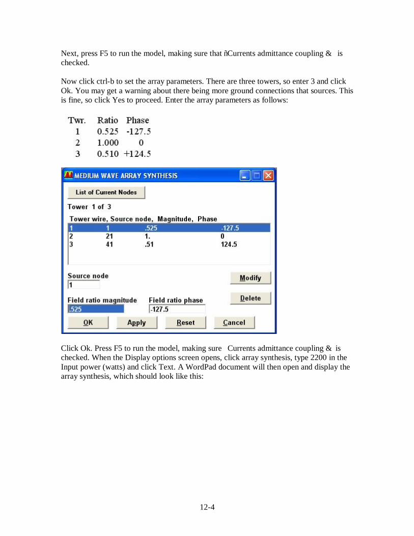
12-4

Next, press F5 to run the model, making sure that “Currents admittance coupling…” is checked. Now click ctrl-b to set the array parameters. There are three towers, so enter 3 and click Ok. You may get a warning about there being more ground connections that sources. This is fine, so click Yes to proceed. Enter the array parameters as follows:

Click Ok. Press F5 to run the model, making sure “Currents admittance coupling…”is checked. When the Display options screen opens, click array synthesis, type 2200 in the Input power (watts) and click Text. A WordPad document will then open and display the array synthesis, which should look like this:

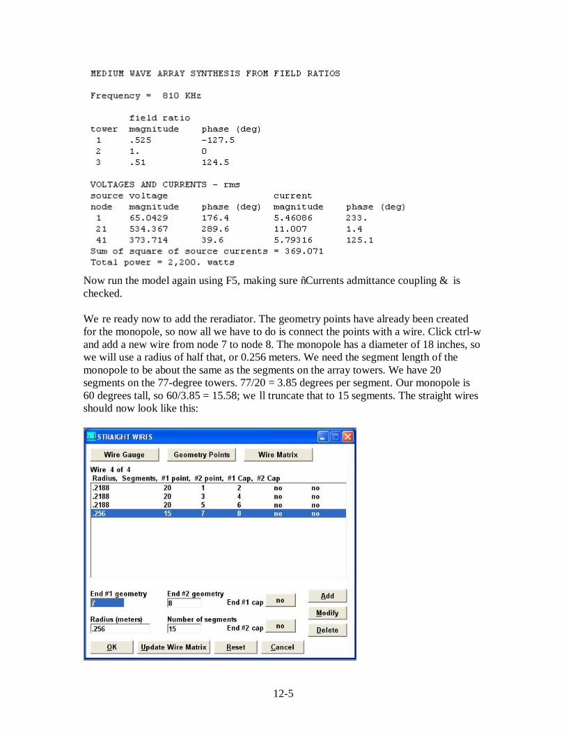
12-5

Now run the model again using F5, making sure “Currents admittance coupling…”is checked. We’re ready now to add the reradiator. The geometry points have already been created for the monopole, so now all we have to do is connect the points with a wire. Click ctrl-w and add a new wire from node 7 to node 8. The monopole has a diameter of 18 inches, so we will use a radius of half that, or 0.256 meters. We need the segment length of the monopole to be about the same as the segments on the array towers. We have 20 segments on the 77-degree towers. 77/20 = 3.85 degrees per segment. Our monopole is 60 degrees tall, so 60/3.85 = 15.58; we’ll truncate that to 15 segments. The straight wires should now look like this:

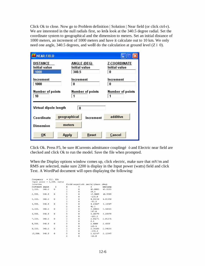
12-6

Click Ok to close. Now go to Problem definition | Solution | Near field (or click ctrl-r). We are interested in the null radials first, so let’s look at the 340.5 degree radial. Set the coordinate system to geographical and the dimension to meters. Set an initial distance of 1000 meters, an increment of 1000 meters and have it calculate out to 10 km. We only need one angle, 340.5 degrees, and we’ll do the calculation at ground level (Z – 0).

Click Ok. Press F5, be sure “Currents admittance coupling…” and Electric near field are checked and click Ok to run the model. Save the file when prompted. When the Display options window comes up, click electric, make sure that mV/m and RMS are selected, make sure 2200 is display in the Input power (watts) field and click Text. A WordPad document will open displaying the following:

12-7

Next, we’ll plot these values on a piece of log-log paper and draw an IDF line at the standard pattern maximum of 20.9. In the example on the following page, the near field plot was started at 100 meters and 100-meter intervals were used to 3 km. 200-meter intervals were used to 4 km, and the radial was then run out to 20 km. The standing wave is clearly visible. This graphical analysis reveals that this particular radial exceeds the standard pattern as a result of the reradiation, indicating that detuning is required. Of course it would be necessary to repeat this E-field analysis on all the proof radials to determine the overall effect of the potential reradiator on the entire pattern. The extent of the pattern distortion is often visible in the radiation pattern, and this is a useful tool to show where the distortion occurs. It is not, however, helpful in determining whether the resultant pattern exceeds the standard pattern. The distortion in the example pattern is clearly visible in the plot below.

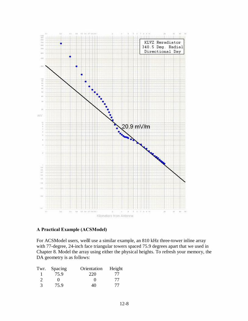
12-8

A Practical Example (ACSModel) For ACSModel users, we’ll use a similar example, an 810 kHz three-tower inline array with 77-degree, 24-inch face triangular towers spaced 75.9 degrees apart that we used in Chapter 8. Model the array using either the physical heights. To refresh your memory, the DA geometry is as follows: Twr. Spacing Orientation Height 1 75.9 220 77 2 0 0 77 3 75.9 40 77

12-9

We’ll model a reradiator, a 200-foot monopole located 1 km from the array reference tower at a bearing of 250 degrees. Calculate the height of the monopole in electrical degrees at 810 kHz:

60360810.0984

200=

÷÷degrees

The distance is 1 km, so use the same equation to calculate the distance in degrees, using 300 as the constant for meters rather than 984 (which we used for feet):

972360810.0300

1000=

÷÷degrees

Set the frequency to 810 kHz (ctrl-f) and create the wires representing the three array towers (ctrl-w). Before we create a wire for the potential reradiator, we must calculate the source voltages for the array towers. The wires of the model should look like this at this point:

Next, type ctrl-b to enter the directional antenna parameters. Select three towers and enter the array parameters as follows:

12-10

Click OK. Press F5 to run the model. When the WordPad window opens, look it over to make sure everything looks okay. Close the WordPad window. We’re ready now to add the reradiator. Click ctrl-w and add a new wire. The monopole has a diameter of 18 inches, so we will use a radius of half that, or 0.256 meters. We need the segment length of the monopole to be about the same as the segments on the array towers. We have 20 segments on the 77-degree towers. 77/20 = 3.85 degrees per segment. Our monopole is 60 degrees tall, so 60/3.85 = 15.58; we’ll truncate that to 15 segments. The straight wires should now look like this:

Click OK to close.

12-11

ACSModel, which was specifically authored for AM broadcast applications, has a feature that makes reradiator analysis a snap. Click Solutions | E and H Fields (or type ctrl-r). That will bring up a window wherein you can plot the E and H fields. Select the Geographic coordinate system, E field and RMS units. Enter 340.5 degrees for the radial. Set the start distance to 1000 meters (1 km), the increment to 1000 meters and have it calculate out to 20 km.

Click OK, then press F5 to run the model. A log-log field strength vs. distance graph will be displayed. Click in the IDF window and enter 20.9, which is the standard pattern inverse distance field on the 340.5 degree radial. The IDF line will move down to 20.9 mV/m and you can see the field strength points as they start well above the IDF line, cross and drop well below the line, then come back up and stabilize right on or just above the line out to 20 km. The analysis shows that there would likely be some significant additive and destructive effects on the field close to the site (inside 4 km), which would probably be observable at the monitor point, and there would be a minimal but unacceptable effect

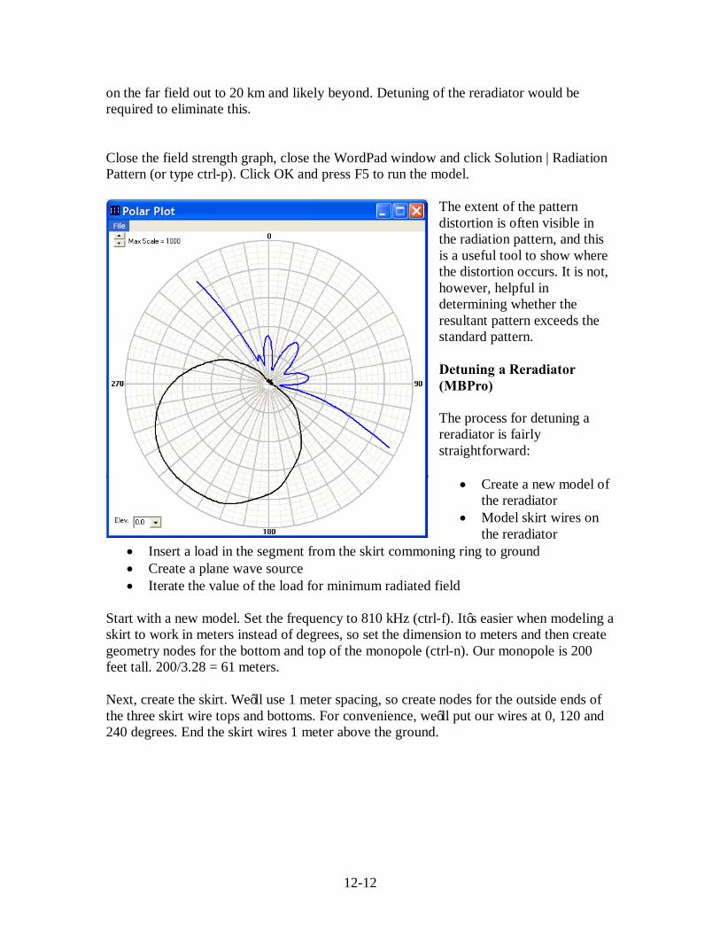
12-12

on the far field out to 20 km and likely beyond. Detuning of the reradiator would be required to eliminate this. Close the field strength graph, close the WordPad window and click Solution | Radiation Pattern (or type ctrl-p). Click OK and press F5 to run the model.

The extent of the pattern distortion is often visible in the radiation pattern, and this is a useful tool to show where the distortion occurs. It is not, however, helpful in determining whether the resultant pattern exceeds the standard pattern. Detuning a Reradiator (MBPro) The process for detuning a reradiator is fairly straightforward:

• Create a new model of the reradiator

• Model skirt wires on the reradiator

• Insert a load in the segment from the skirt commoning ring to ground • Create a plane wave source • Iterate the value of the load for minimum radiated field

Start with a new model. Set the frequency to 810 kHz (ctrl-f). It’s easier when modeling a skirt to work in meters instead of degrees, so set the dimension to meters and then create geometry nodes for the bottom and top of the monopole (ctrl-n). Our monopole is 200 feet tall. 200/3.28 = 61 meters. Next, create the skirt. We’ll use 1 meter spacing, so create nodes for the outside ends of the three skirt wire tops and bottoms. For convenience, we’ll put our wires at 0, 120 and 240 degrees. End the skirt wires 1 meter above the ground.

12-13

Now we’ll create the wires for the monopole and skirt (ctrl-w). Connect nodes 1 and 2 with a radius of 0.256 and 15 segments for the monopole. For the skirt wires, we’ll use 1/2-inch wires (0.006 meters). The short segments between monopole and skirt wires, from wire to wire (commoning ring) and from commoning ring to ground will have one segment each. The skirt wires themselves will have 15 segments like the monopole. Connect nodes 2 and 3 for the monopole top to the north skirt wire. Connect nodes 3 and 4 for the north skirt wire. Connect nodes 2 and 5 for the monopole top to the southeast skirt wire. Connect nodes 5 and 6 for the southeast skirt wire. Connect nodes 2 and 7 for the monopole top to the southwest skirt wire. Connect nodes 7 and 8 for the southwest skirt wire. Now build the commoning ring by connecting nodes 4, 6 and 8. A final wire is needed from the commoning ring to ground, so connect nodes 4 and 1. The wire table should look like this:

12-14

We can confirm the model geometry by looking at a 3D view. Click Diagnostics | 3D display (or press F3). Zoom in and rotate to see the monopole and skirt wires. Now we will place a load at the bottom of the skirt. Type ctrl-l and create a load with an R of 0 and an X of -j100 at node 71 (bottom of the skirt). The value of this load will be iterated to detune the monopole.

12-15

Now we’ll create a plane wave source. Press F11 and create a source with a zenith of 90, azimuth of zero, phase of zero and an incident field of 10 volts.

Type ctrl-p and set up a radiation sweep at a single zero zenith and a 72-radial 5-degree increment azimuth. Press F5 to run the model. Make sure that Currents and Radiation pattern are checked. When the Display options window opens, click Scattered Fields mV/m, type 1000 in the Radial distance window and click Text. A WordPad window will open. Note the E-theta values for the ND pattern is approximately 88 mV/m. Close the window. Now iterate the load value (ctrl-l) and use F5 to re-run the model. A value of –j289 results in a reradiated field of 0.229 mV/m with a 10-volt incident plane wave. We can consider that detuned. A skirt and detuning network can now be designed using the model results. If desired, the detuned reradiator can be modeled into the array model, but this is a lot of work. It is recommended that you do this using meters as the units and that you map out all the geometry nodes on a piece of paper before attempting to construct the model. Be sure to build and synthesize the directional array before bringing in the detuned reradiator. For our example, here are the node list and wire table for the array with the skirted and detuned reradiator.

12-16

Note that the units are meters and the coordinate system is spherical. It is possible to model a skirted reradiator using the geographic coordinate system, but the angles tend to become very small, leading to problems with precision. Consider that in this case, with the reradiator 1 km distant, the azimuth difference between the reradiator itself and the endpoints of the skirt wires is .051 degrees and the distance difference between the reradiator and the endpoints of the skirt wires is 0.332 meters. The reality is that more precision than that is really required to precisely place the

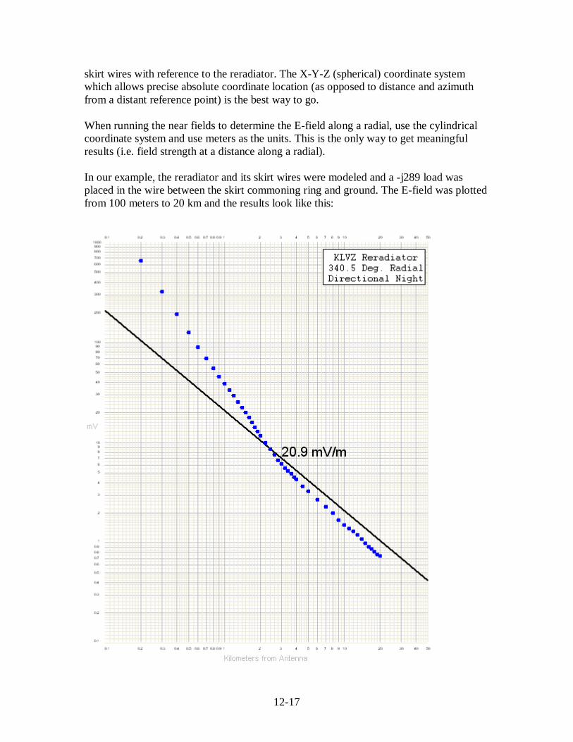
12-17

skirt wires with reference to the reradiator. The X-Y-Z (spherical) coordinate system which allows precise absolute coordinate location (as opposed to distance and azimuth from a distant reference point) is the best way to go. When running the near fields to determine the E-field along a radial, use the cylindrical coordinate system and use meters as the units. This is the only way to get meaningful results (i.e. field strength at a distance along a radial). In our example, the reradiator and its skirt wires were modeled and a -j289 load was placed in the wire between the skirt commoning ring and ground. The E-field was plotted from 100 meters to 20 km and the results look like this:

12-18

Note how nicely the IDF settles down below standard pattern beyond 2.5 km or so. Also note how the IDF is well above standard pattern inside 2.5 km. Were a monitor point located within that distance on the radial, it would likely indicate a high value that would bear no relationship to what is really going on along the radial in the far field, where it counts. Going back to the graph on page 11-8 representing the same radial with a non-detuned reradiator in what amounts to a worst-case situation, note that while the far field IDF does exceed standard pattern by a bit, the excursion is not very much. This says something about the effect of even a worst-case reradiator on a real-world pattern. The measurement points likely to be used in a conventional proof of performance would show high ratios indicating a radial IDF far in excess of standard pattern when the reality is that it is only 0.8 dB high. All this is simply to say that while the FCC does require that reradiation be treated so as to prevent exceeding the standard pattern, the likelihood of reradiation actually causing interference to another allocation is slim indeed.