Alternatives to Randomized Trials; P-values and Confidence Intervals

Tom Newman

November 17, 2011

Lec 8 Alts to RCTs P values and CI 16Nov11

Announcements

Lots of supplemental reading on website Exam questions: due in section today Next Thursday is Thanksgiving Take-home final will be handed out and

posted after section (or maybe that night) 12/1, discussed in lecture 12/8

No section 12/8

Outline Alternatives to RCTs

– Instrumental variables and natural experiments – more examples

– Measuring alternate variables to estimate bias• Predictor• Outcome

– Propensity scores P-values and Confidence Intervals

– What they don’t and do mean– CI for negative studies– CI for small numerators

Other Instrumental variable examples

Distance from residence to hospital that does a procedure

Medication choice of MD for the previous patient with similar indications

Phototherapy use in birth hospital (Biostat 215)

Problem 10.1: Thimerosal and autism

More natural experiments: Effect of increased ED copayment: 23%

decrease in ED visits with a $50-100 ED copayment, led to decreased hospital admissions without an increase in deaths or ICU admissions*

Aircraft cabin air recirculation and symptoms of the common cold: no difference by type of air recirculation in aircraft **

*Hsu J, et al. Health Services Research 2006;41:1801-20

** Zitter JN et al. JAMA 2002;288:483-6

Measuring alternate variables to estimate bias or confounding

Measure a predictor that would cause the same bias as the predictor of interest (and see if it does)

Measure an outcome that would be affected by bias, but not by treatment of interest (and see if it is)

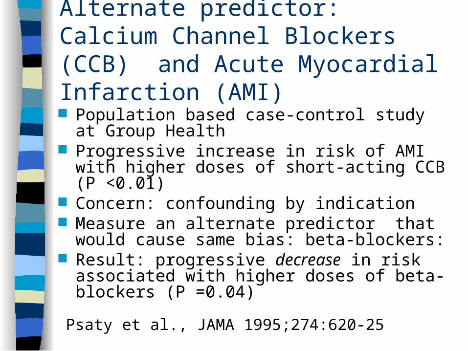
Alternate predictor: Calcium Channel Blockers (CCB) and Acute Myocardial Infarction (AMI) Population based case-control study at Group

Health Progressive increase in risk of AMI with

higher doses of short-acting CCB (P <0.01) Concern: confounding by indication Measure an alternate predictor that would

cause same bias: beta-blockers: Result: progressive decrease in risk

associated with higher doses of beta-blockers (P =0.04)

Psaty et al., JAMA 1995;274:620-25

Suicide Risk in Bipolar Disorder During Treatment With Lithium and Divalproex

Retrospective cohort study of Kaiser Permanente and Group Health patients with bipolar disorder

Compared with no treatment, patients treated with divalproex at 2.1 times suicide risk

Concern: confounding by indication Results: Suicides per 1000 person/years

– 31.3 for treatment with divalproex– 15 for no treatment (P<0.001)– 10.8 for Lithium (P<0.001)

If confounding by indication, expect same bias for Lithium

Goodwin et al. JAMA. 2003;290:1467-1473

Initial Mood Stabilizer Prescription by Year of Initial Diagnosis

Goodwin et al. JAMA. 2003;290:1467-1473

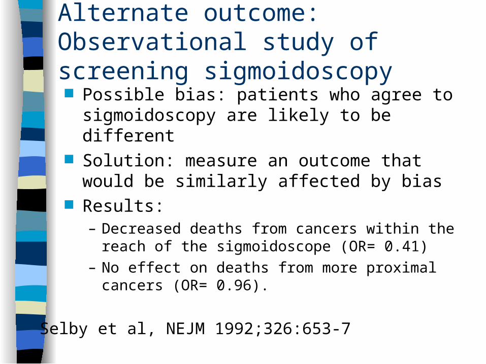
Alternate outcome: Observational study of screening sigmoidoscopy Possible bias: patients who agree to

sigmoidoscopy are likely to be different Solution: measure an outcome that would be

similarly affected by bias Results:

– Decreased deaths from cancers within the reach of the sigmoidoscope (OR= 0.41)

– No effect on deaths from more proximal cancers (OR= 0.96).

Selby et al, NEJM 1992;326:653-7

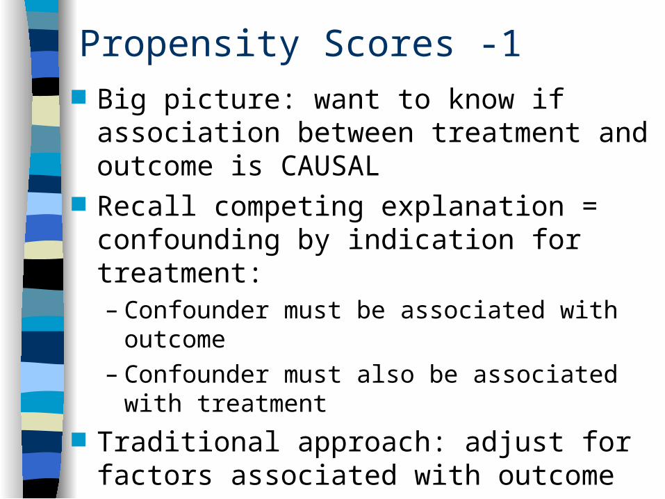
Propensity Scores -1 Big picture: want to know if association

between treatment and outcome is CAUSAL

Recall competing explanation = confounding by indication for treatment:– Confounder must be associated with outcome– Confounder must also be associated with

treatment Traditional approach: adjust for factors

associated with outcome

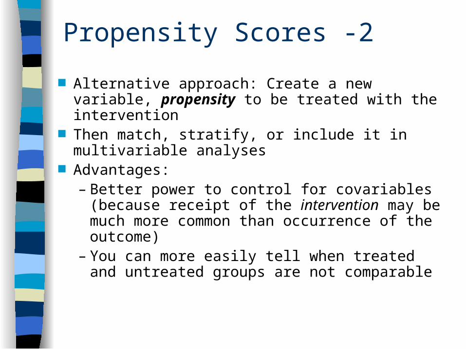
Propensity Scores -2

Alternative approach: Create a new variable, propensity to be treated with the intervention

Then match, stratify, or include it in multivariable analyses

Advantages:– Better power to control for covariables (because

receipt of the intervention may be much more common than occurrence of the outcome)

– You can more easily tell when treated and untreated groups are not comparable

How Much Overlap In The Propensity Scores Do We Want?

0

1

Not TreatedTreated

Propensity toreceive treatment

0

1

Not TreatedTreated

Propensity toreceive treatment

0

1

Not TreatedTreated

Propensity toreceive treatment

www.chrp.org

Example: Aspirin use and all-cause mortality among patients being evaluated for known or suspected Coronary Artery Disease

RQ: Does aspirin reduce all-cause mortality in patients with coronary disease

Design: Cohort study Subjects: 6174 consecutive patients getting

stress echocardiograms Predictor: Aspirin use Outcome: All-cause mortality Crude result: 4.5% mortality in each group

Gum PA et al. JAMA 2001; 286: 1187-94

Analysis using Propensity Scores

Two multivariable analyses:– Predictors of aspirin use– Predictors of death

Use predictors of ASA use to create a propensity score

Users and non-users of ASA matched on ASA propensity score

Compare mortality in matched groups (Unmatched patients cannot be analyzed)

Survival in Propensity-Matched Patients

Recall total N=6174

Proton pump inhibitor use and risk of adverse cardiovascular events in aspirin treated patients with first time myocardial infarction: nationwide propensity score matched study*

*Charlot M et al. BMJ. 2011 May 11;342:d2690

Fig 3. Time dependent adjusted propensity score matched Cox proportional hazard analysis of risk of cardiovascular death, myocardial infarction, or stroke for subtypes of proton pump inhibitors and H2 receptor blockers

Alternate predictor: H2 blocker

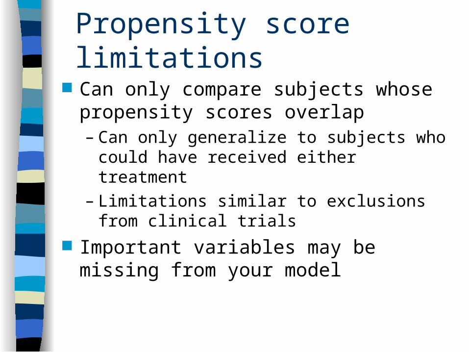
Propensity score limitations

Can only compare subjects whose propensity scores overlap– Can only generalize to subjects who could

have received either treatment– Limitations similar to exclusions from

clinical trials Important variables may be missing

from your model

Questions?

Understanding P-values and Confidence Intervals (Chapter 11)

Additional Recommended Reading See syllabus Articles by Steven

Goodman

Why cover this material here? P-values and confidence intervals are

ubiquitous in clinical research Widely misunderstood and mistaught Your biostatistics course now gets it

right, but experience suggests some people have trouble and appreciate additional time

Pedagogical argument:– Is it important?– Can you handle it?

Example: Douglas Altman Definition of 95% Confidence Intervals*

"A strictly correct definition of a 95% CI is, somewhat opaquely, that 95% of such intervals will contain the true population value.

“Little is lost by the less pure interpretation of the CI as the range of values within which we can be 95% sure that the population value lies.”

*Quoted in: Guyatt, G., D. Rennie, et al. (2002). Users' guides to the medical literature : essentials of evidence-based clinical practice. Chicago, IL, AMA Press.

Understanding P-values and confidence intervals is important because It explains things that otherwise do not

make sense, e.g. the importance of stating hypotheses in advance and correction for multiple hypothesis testing

You will be using them all the time You are future leaders in clinical

research

You can handle it because

We have already covered the important concepts at length earlier in this course– Prior probability– Posterior probability– What you thought before + new

information = what you think now We will support you through the process

Review of traditional statistical significance testing

State null (Ho) and alternative (Ha) hypotheses

Choose α Calculate value of test statistic from

your data Calculate P- value from test statistic If P-value < α, reject Ho

Problem:

Traditional statistical significance testing has led to widespread misinterpretation of P-values

What P-values don’t mean

If the P-value is 0.05, there is a 95% probability that…– The results did not occur by chance– The null hypothesis is false– There really is a difference between the

groups

So if P = 0.05, what IS there a 95% probability of?

Recall false-negative confusion from last week:

Sensitivity of CT scan for sub-arachnoid hemorrhage (SAH) is 90%

Therefore, false negative rate is 10% 10% chance of missing SAH is too high Therefore, always do a lumbar puncture

The Problem

  Disease No Disease  

Test + TP FP TP+FP

Test - FN TN FN+TN

Total TP+FN FP+TN N

The numerator for the false negative rate is clear, but the denominator is not

The Problem

  Disease No Disease  

Test + TP FP TP+FP

Test - FN TN FN+TN

Total TP+FN FP+TN N

Sensitivity and specificity go this way:

The Problem

  Disease No Disease  

Test + TP FP TP+FP

Test - FN TN FN+TN

Total TP+FN FP+TN N

When in clinical medicine we need to go this way, to get predictive value:

The same error happens with false-positives, e.g.

If specificity is 95%, then The false-positive rate is 5%. Therefore, if the patient has a positive result,

there’s a 5% chance it is a false positive Therefore, if the patient tests positive, there’s

a 95% probability that it is a true positive and that she has the disease

Statistical Significance Testing

 Real

DifferenceNo Difference

(H0)

Study + 1-

Study - 1-

is like the (1-specificity) false-positive rate It is the maximum probability of a Type I (false

positive) error CONDITIONAL on the null hypothesis So saying P < 0.05 means the probability of a true

difference is 95% is like saying specificity of 95% means positive predictive value is 95%

CONFIDENCE INTERVALS

What Confidence Intervals don’t mean

There is a 95% chance that the true value is within the interval

If you conclude that the true value is within the interval you have a 95% chance of being right

The range of values within which we can be 95% sure that the true population value lies

One source of confusion: Statistical “confidence”

(Some) statisticians say: “You can be 95% confident that the population value is in the interval.”

This is NOT the same as “There is a 95% probability that the population value is in the interval.”

“Confidence” is tautologously defined by statisticians as what you get from a confidence interval

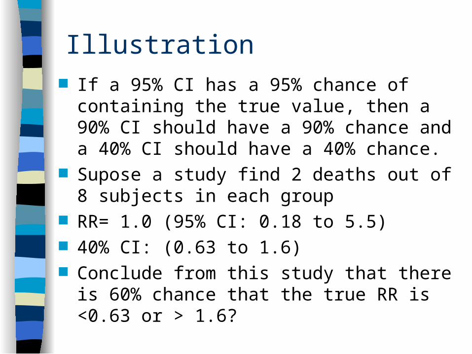
Illustration If a 95% CI has a 95% chance of containing

the true value, then a 90% CI should have a 90% chance and a 40% CI should have a 40% chance.

Supose a study find 2 deaths out of 8 subjects in each group

RR= 1.0 (95% CI: 0.18 to 5.5) 40% CI: (0.63 to 1.6) Conclude from this study that there is 60%

chance that the true RR is <0.63 or > 1.6?

Confidence Intervals apply to a Process

Consider a bag with 19 white and 1 pink grapefruit

The process of selecting a grapefruit at random has a 95% probability of yielding a white one

But once I’ve selected one, does it still have a 95% chance of being white?

You may have prior knowledge that changes the probability (e.g., pink grapefruit have thinner peel are denser, etc.)

Confidence Intervals for negative studies: 5 levels of sophistication

Example 1: Oral amoxicillin to treat possible occult bacteremia in febrile children*– Randomized, double-blind trial– 3-36 month old children with T≥ 39º C (N=

955)– Treatment: Amox 125 mg/tid (≤ 10 kg) or

250 mg tid (> 10 kg) (tid=3x/day)– Outcome: “major infectious morbidity”

*Jaffe et al., New Engl J Med 1987;317:1175-80

Amoxicillin for possible occult bacteremia 2: Results

Bacteremia in 19/507 (3.7%) with amox, vs 8/448 (1.8%) with placebo (P=0.07)

“Major Infectious Morbidity” 2/19 (10.5%) with amox vs 1/8 (12.5%) with placebo (P = 0.9)

Conclusion: “Data do not support routine use of standard doses of amoxicillin…”

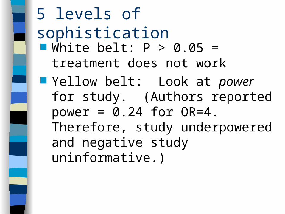
5 levels of sophistication White belt: P > 0.05 = treatment does

not work Yellow belt: Look at power for study.

(Authors reported power = 0.24 for OR=4. Therefore, study underpowered and negative study uninformative.)

5 levels of sophistication, cont’d Green belt: Look at 95% CI!

– Authors calculated OR= 1.2 (95% CI: 0.02 to 30.4)– This is based on 1/8 (12.5%) with placebo vs 2/19

(10.5%) with amox– (They put placebo on top)– (Silly to use OR)

With amox on top, RR = 0.84 (95% CI: 0.09 to 8.0)

This was the sophistication level of TBN in a letter to the editor (with Bob Pantell in 1987)

5 levels of sophistication, cont’d Blue belt: Make sure you do an

“intention to treat” analysis! – It is not OK to restrict attention to

bacteremic patients– So it should be 2/507 (0.39%) with amox

vs 1/448 (0.22%) with placebo– RR= 1.8 (95% CI: 0.16 to 19.4)

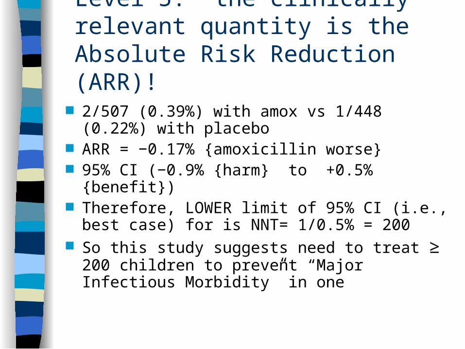
Level 5: the clinically relevant quantity is the Absolute Risk Reduction (ARR)!

2/507 (0.39%) with amox vs 1/448 (0.22%) with placebo

ARR = −0.17% {amoxicillin worse} 95% CI (−0.9% {harm} to +0.5% {benefit}) Therefore, LOWER limit of 95% CI (i.e., best

case) for is NNT= 1/0.5% = 200 So this study suggests need to treat ≥ 200

children to prevent “Major Infectious Morbidity” in one

Stata output. csi 2 1 505 447

| Exposed Unexposed | Total

-----------------+------------------------+----------

Cases | 2 1 | 3

Noncases | 505 447 | 952

-----------------+------------------------+----------

Total | 507 448 | 955

| |

Risk | .0039448 .0022321 | .0031414

| |

| Point estimate | [95% Conf. Interval]

|------------------------+----------------------

Risk difference | .0017126 | -.005278 .0087032

Risk ratio | 1.767258 | .1607894 19.42418

Attr. frac. ex. | .4341518 | -5.219315 .9485178

Attr. frac. pop | .2894345 |

+-----------------------------------------------

chi2(1) = 0.22 Pr>chi2 = 0.6369

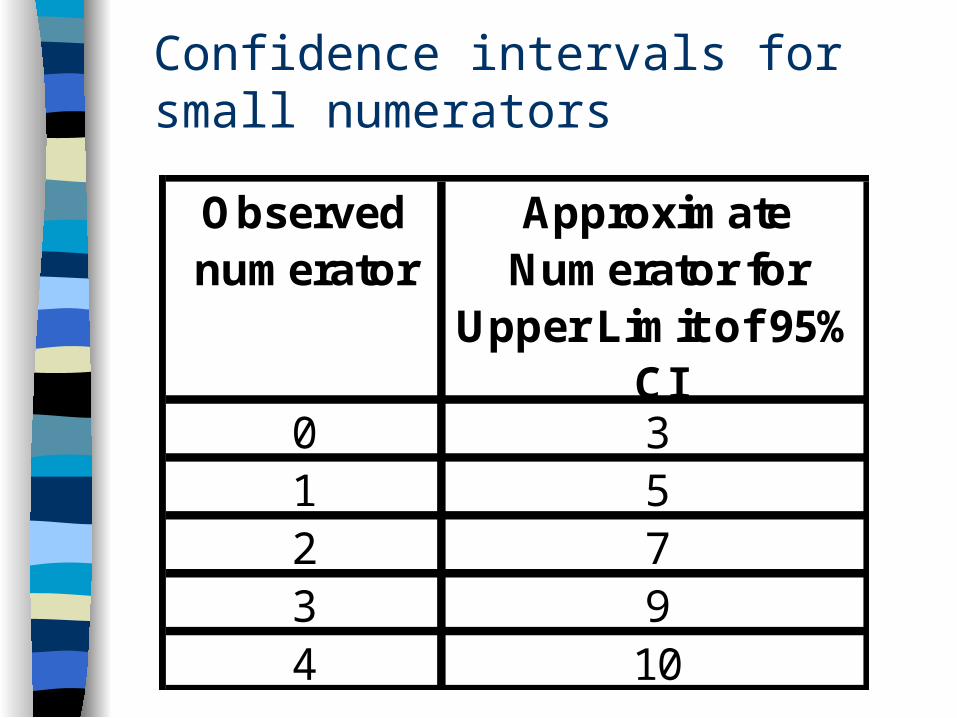
Confidence intervals for small numerators

Observed numerator

Approximate Numerator for

Upper Limit of 95% CI

0 31 52 73 94 10

Example 1

A study finds 1 person with a serious adverse effect among 50 studied. What is the upper limit of the 95% CI?

Estimate: 5/50 = 10% Actual: 10.6%

Example 2

A study reports sensitivity of 97% in a sample in which 100 people have the disease. What is the LOWER limit of the 95% CI for sensitivity?– False negatives: 3/100– Estimate upper limit of 95% CI for FN = 9/100– Estimate lower 95% CI for sensitivity = 91%– Actual 91.4%

Additional examples

Problem 10.1 RQ: Do small doses of mercury in the vaccine

preservative thimerosal cause autism? Data source: electronic data from a large HMO (very

high N) Opportunity:

– Rhogam (Rh Immune Globulin) is given to Rh-negative women during pregnancy (if they get good prenatal care)

– It had 25 mcg of Hg per dose until 2001– You have data from a electronic records, 1990 to the present,

with blood types, Rhogam exposure and diagnoses of autism Assume:

– You are interested in effects of 25 mcg of Hg– The incidence of autism has been increasing

How would you design your study? What groups would you compare?

Problem 10.5 Does perioperative use of lipid-lowering

drugs decrease mortality following cardiac surgery?

Example 2: Pyelonephritis and new renal scarring in the International Reflux Study in Children*

RCT of ureteral reimplantation vs prophylactic antibiotics for children with vesicoureteral reflux

Overall result: surgery group fewer episodes of pyelonephritis (8% vs 22%; NNT = 7; P < 0.05) but more new scarring (31% vs 22%; P = .4)

This raises questions about whether new scarring is caused by pyelonephritis

Weiss et al. J Urol 1992; 148:1667-73

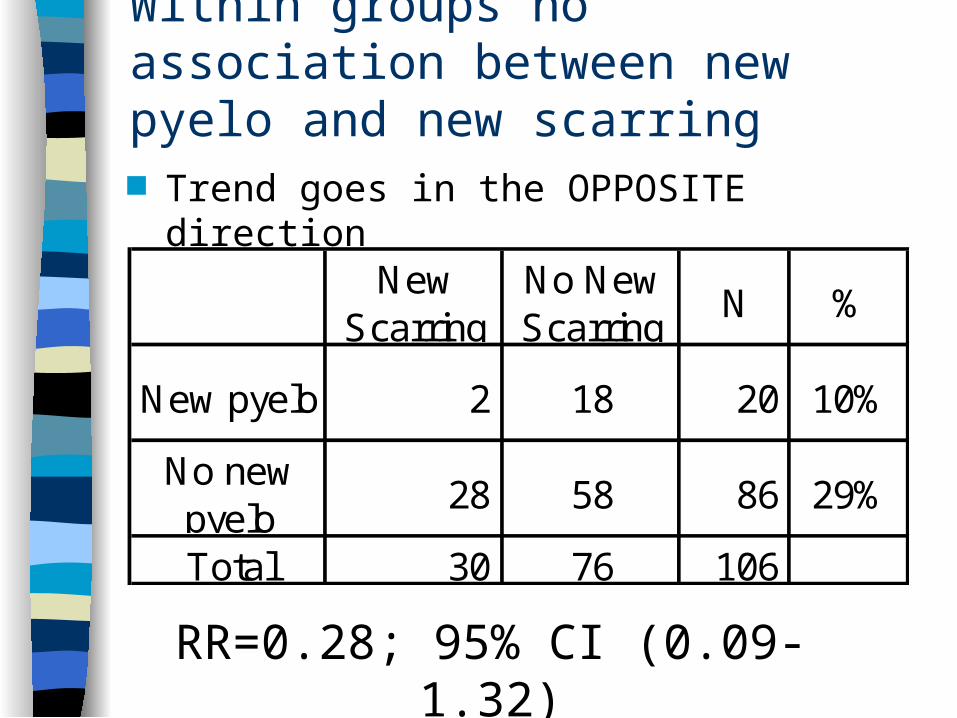
Within groups no association between new pyelo and new scarring

Trend goes in the OPPOSITE direction

RR=0.28; 95% CI (0.09-1.32)Weiss, J Urol 1992:148;1672

New Scarring

No New Scarring

N %

New pyelo 2 18 20 10%

No new pyelo

28 58 86 29%

Total 30 76 106

Stata output to get 95% CI:

. csi 2 18 28 58 | Exposed Unexposed | Total-----------------+------------------------+------------ Cases | 2 18 | 20 Noncases | 28 58 | 86-----------------+------------------------+------------ Total | 30 76 | 106 | | Risk | .0666667 .2368421 | .1886792 | | | Point estimate | [95% Conf. Interval] |------------------------+------------------------ Risk difference | -.1701754 | -.3009557 -.0393952 Risk ratio | .2814815 | .069523 1.13965 Prev. frac. ex. | .7185185 | -.1396499 .930477 Prev. frac. pop | .2033543 | +----------------------------------------- chi2(1) = 4.07 Pr>chi2 = 0.0437

Conclusions

No evidence that new pyelonephritis causes scarring

Some evidence that it does not P-values and confidence intervals are

approximate, especially for small sample sizes There is nothing magical about 0.05

Key concept: calculate 95% CI for negative studies– ARR for clinical questions (less generalizable)

– RR for etiologic questions

When P-values and Confidence Intervals Disagree

Usually P < 0.05 means 95% CI excludes null value But both 95% CI and P-values are based on

approximations, so this may not be the case Illustrated by International Reflux Study slide above If you want 95% CI and P- values to agree, use “test-

based” confidence intervals – see next slide

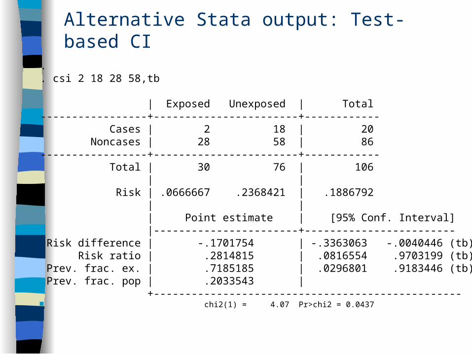
Alternative Stata output: Test-based CI

.

. csi 2 18 28 58,tb

| Exposed Unexposed | Total-----------------+-----------------------+------------ Cases | 2 18 | 20 Noncases | 28 58 | 86-----------------+-----------------------+------------ Total | 30 76 | 106 | | Risk | .0666667 .2368421 | .1886792 | | | Point estimate | [95% Conf. Interval] |-----------------------+------------------------ Risk difference | -.1701754 | -.3363063 -.0040446 (tb) Risk ratio | .2814815 | .0816554 .9703199 (tb) Prev. frac. ex. | .7185185 | .0296801 .9183446 (tb) Prev. frac. pop | .2033543 | +------------------------------------------------- chi2(1) = 4.07 Pr>chi2 = 0.0437

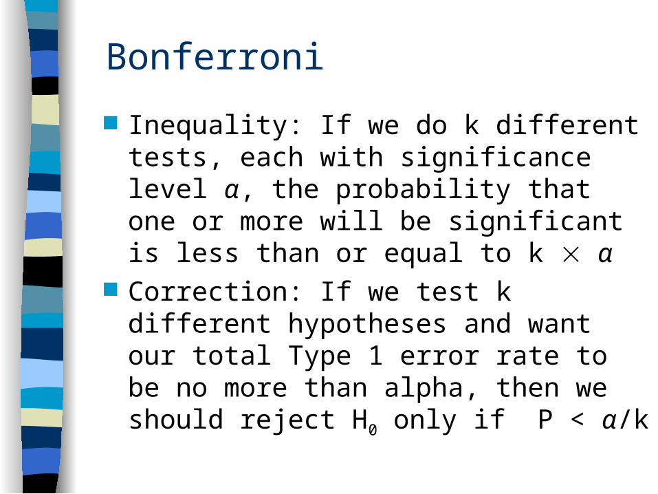
Bonferroni

Inequality: If we do k different tests, each with significance level α, the probability that one or more will be significant is less than or equal to k α

Correction: If we test k different hypotheses and want our total Type 1 error rate to be no more than alpha, then we should reject H0 only if P < α/k

Derivation

Let A & B = probability of a Type 1 error for hypotheses A and B

P(A or B) = P(A) + P(B) – P(A & B) Under Ho, P(A) = P(B) = α So P(A or B) = α + α - P(A & B) = 2α - P(A & B). Of course, it is possible to falsely reject 2 different null

hypotheses, so P(A & B) > 0. Therefore, the probability of falsely rejecting either of the null hypotheses must be less than 2α.

Note that often A & B are not independent, in which case Bonferroni will be even more excessively conservative

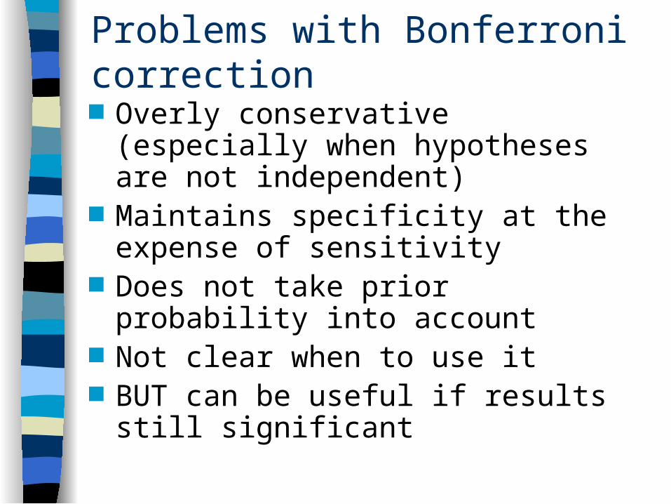
Problems with Bonferroni correction

Overly conservative (especially when hypotheses are not independent)

Maintains specificity at the expense of sensitivity

Does not take prior probability into account

Not clear when to use it BUT can be useful if results still

significant