Alternative Beta
64
EDITOR’S LETTER Hossein Kazemi WHAT A CAIA MEMBER SHOULD KNOW Alternative Beta: Redefining Alpha and Beta Soheil Galal, Rafael Silveira, and Alison Rapaport RESEARCH REVIEW OPEC Spare Capacity, the Term Structure of Oil Futures Prices, and Oil Futures Returns Hilary Till FEATURED INTERVIEW Mebane Faber on ETFs NEWS AND VIEWS The Time Has Come for Standardized Total Cost Disclosure for Private Equity Andrea Dang, David Dupont, and Mike Heale CAIA MEMBER CONTRIBUTION The Hierarchy of Alpha Christopher M. Schelling, CAIA INVESTMENT STRATEGIES Private Market Real Estate Investment Options for Defined Contribution Plans: New and Improved Solutions Jani Venter and Catherine Polleys PERSPECTIVES M&A Activity: Where Are We In the Cycle? Fabienne Cretin, Stéphane Dieudonné, and Slimane Bouacha Nowcasting: A Risk Management Tool Alexander Ineichen, CAIA VC-PE INDEX Mike Nugent and Mike Roth THE IPD GLOBAL INTEL REPORT Max Arkey Chartered Alternative Investment Analyst Association ® Q3 2015, Volume 4, Issue 2 Alternative Investment Analyst Review
Transcript of Alternative Beta

EDITOR’S LETTERHossein Kazemi
WHAT A CAIA MEMBER SHOULD KNOWAlternative Beta: Redefining Alpha and BetaSoheil Galal, Rafael Silveira, and Alison Rapaport
RESEARCH REVIEWOPEC Spare Capacity, the Term Structure of Oil Futures Prices, and Oil Futures ReturnsHilary Till
FEATURED INTERVIEWMebane Faber on ETFs
NEWS AND VIEWSThe Time Has Come for Standardized Total Cost Disclosure for Private EquityAndrea Dang, David Dupont, and Mike Heale
CAIA MEMBER CONTRIBUTIONThe Hierarchy of AlphaChristopher M. Schelling, CAIA
INVESTMENT STRATEGIESPrivate Market Real Estate Investment Options for Defined Contribution Plans: New and Improved SolutionsJani Venter and Catherine Polleys
PERSPECTIVESM&A Activity: Where Are We In the Cycle?Fabienne Cretin, Stéphane Dieudonné, and Slimane Bouacha
Nowcasting: A Risk Management ToolAlexander Ineichen, CAIA
VC-PE INDEXMike Nugent and Mike Roth
THE IPD GLOBAL INTEL REPORTMax Arkey
Chartered Alternative Investment Analyst Association®Q3 2015, Volume 4, Issue 2
Alternative Investment Analyst Review

Call for ArticlesArticle submissions for future issues of Alternative Investment Analyst Review (AIAR) are always welcome. Articles should cover a topic of interest to CAIA members and should be single-spaced. Additional information on submissions can be found at the end of this issue. Please email your submission or any questions to [email protected]. Chosen pieces will be featured in future issues of AIAR, archived on CAIA.org, and promoted throughout the CAIA community.

Editor’s Letter
1Editor’s Letter
Efficiently Inefficient
The efficiency of market prices is one of the central questions in financial economics. The central thesis is that security markets are perfectly efficient, but this leads to two paradoxes: First, no one has an incentive to collect information in an efficient market, so how does the market become efficient? Second, if asset markets are efficient, then positive fees to active managers implies inefficient markets for asset management. In other words, one cannot simultaneously assume that financial markets are dominated by rational investors who arbitrage away pricing inefficiencies and that there are irrational people who invest with professional money managers who according to efficient market hypothesis (EMH) do not add any value. Why should professional money managers exist at all, and why should some investors be willing to pay them substantial fees to manage their assets?
The presence of active money managers seems to imply that markets are not efficient as thousands of hedge funds, private equity funds, and active mutual funds earn substantial fees when, according to EMH, they should underperform active strategies on an after-fee basis. However, if markets were highly inefficient, many more people would enter the active money management business to earn a portion of those fees and in the process help make markets more efficient. Therefore, it seems that there must be a fine balance between efficiency and inefficiency. Lasse Heje Pedersen calls this situation “efficiently inefficient.”
Efficiently inefficient presents the idea that markets are, on average, just inefficient enough to compensate managers and investors for their costs and risks, but not so inefficient as to present a large number of money managers with low hanging fruit. Therefore, the flow of capital to active management is limited in a world that is efficiently inefficient. In such a world, competition among active money managers results in markets that are almost efficient, but some inefficiencies exist that reward those who can identify and exploit them.
Pedersen argues that professional asset managers arise naturally as a result of the returns to scale in collecting and trading on information. They collect information about securities and then invest on this information on behalf of others. Therefore, professional asset managers are central to understanding market efficiency. In a market characterized as being efficiently inefficient, there exist a limited number of market inefficiencies that can be exploited by some money managers. However, finding the right manager takes time and resources, and, therefore, investors have to decide whether to spend search costs to find an active asset manager or allocate their capital to a passive strategy. At the margin, investors become indifferent between passive strategies and searching for an active asset manager. If search costs are low, such that investors easily can identify good managers, then more money is allocated to active management and some pricing inefficiencies are arbitraged away.
Of course, there are investors who lack the resources, the patience or the skills to search for good active managers, and as a result, they allocate randomly to both good and bad managers. In fact, one can argue that these “noise allocators,” as Pedersen calls them, are more likely to invest with bad managers, because the skilled managers tend to have capacity constraints. The performance of noise allocators will depend on their relative allocations to good and bad managers, but their overall performance after fees is likely to be worse than that of passive investment. In addition, if noise allocators represent a relative large proportion of investors, then the overall performance of active managers is likely to be worse than that of passive managers.
Hossein Kazemi Editor

Table of Contents
Alternative Investment Analyst ReviewSummer • 2015
2
What a CAIA Member Should KnowAlternative Beta: Redefining Alpha and Beta. . . . . . . . . . . . . . . . . . . . . . . . . . . . . . . . . . . . . 5By Soheil Galal, Rafael Silveira and Alison Rapaport JP Morgan
ABSTRACT: Alternative beta strategies extend the concept of “beta investing” from long-only traditional strategies to strategies that include both long and short investing. Although alternative beta approaches have relevance for different categories of alternatives, this article focuses on hedge fund strategies and describes what portfolio managers and investors should know about “alt beta” in that context.
Research ReviewOPEC Spare Capacity, the Term Structure of Oil Futures Prices, and Oil Futures Returns . . . . . . . . . . . . . . . . . . . . . . . . . . . . . . . . . . . . . . . . . . . . . . . . . . . . . . . . . . . . . . . . . . . . . . . . . . . 10By Hilary Till Premia Research LLC; and EDHEC-Risk Institute
ABSTRACT: In this article, the author asks if we can explain in simple terms whether holding long futures positions in crude oil is a wise decision or not. It turns out that knowing whether OPEC spare capacity is at comfortable levels or not would have been very helpful in making this decision, at least since the 1990s. But this factor alone is not sufficient. One has to also examine the shape of the crude oil futures curve. The article provides details on various scenarios and examines how the author came to these conclusions.
Featured InterviewMebane Faber on ETFs . . . . . . . . . . . . . . . . . . . . . . . . . . . . . . . . . . . . . . . . . . . . . . . . . . . . . . . 20
ABSTRACT: AIAR interviews Mebane Faber, co-founder and Chief Investment Officer of Cambria Investment Management and author of numerous white papers and three books: Shareholder Yield, The Ivy Portfolio, and Global Asset Allocation. In this interview he descibes his work at Cambria on ETFs and his views on the CAIA designation.
News and ViewsThe Time Has Come for Standardized Total Cost Disclosure for Private Equity. . . . . . . . 23By Andrea Dang, David Dupont, and Mike Heale CEM Benchmarking, Inc
ABSTRACT: Given the level of detail and timing of private equity manager reports, can pension funds disclose investment costs in a consistent manner across the industry? What would full cost disclosure require of a pension fund? The authors found a good example of this in one of their benchmarking clients and describe their perspective in this article.
CONTACT USU.S. +1 413 253 7373Hong Kong +852 3655 0568
Singapore +65 6536 4241Email [email protected]
CAIA.org
AIAR STAFFHossein Kazemi Keith Black Editors
Barbara J. Mack Content Director
Angel Cruz Creative and Design
FOLLOW US

Table of Contents
3Table of Contents
CAIA Member ContributionThe Hierarchy of Alpha . . . . . . . . . . . . . . . . . . . . . . . . . . . . . . . . . . . . . . . . . . . . . . . . . . . . . . . . . . . . . . . . . . . . . . . . . . 29By Christopher M. Schelling, CAIA Texas Municipal Retirement System
ABSTRACT: Hedge funds and private equity funds have had their share of detractors over the last few years, with many institutional investors questioning whether the returns they have generated justify the significantly higher fees paid. Certainly, on a relative performance basis, a large number of these funds have had a tough time keeping up with long-only equities. There is also no debate that alternatives have become a much more competitive sector. This article evaluates the evolution of the industry and provides insight on how institutional investors should approach the question of manager selection and performance.
Investment StrategiesPrivate Market Real Estate Investment Options for Defined Contribution Plans: New and Improved Solutions . . . . . . . . . . . . . . . . . . . . . . . . . . . . . . . . . . . . . . . . . . . . . . . . . . . . . . . . . . . . . . . . . . . . . . . . . . . . . . . . . . . . . . . . . . . . . . . 33By Jani Venter and Catherine Polleys Aon Hewitt Investment Consulting
ABSTRACT: Historically, investment vehicles using private real estate have been largely unavailable to defined contribution (“DC”) plan participants, but that is now changing. The maturation of daily-valued private real estate funds along with a shift in DC plans towards the use of multi-asset portfolios such as custom target date and objective-based funds have introduced a new investment environment. With these products, daily-priced real estate funds that address legacy vehicle concerns are now available, DC investors can incorporate the return profile and diversification benefits of private core real estate into their multi-asset class investment portfolios. This article assesses the utility of private real estate funds in the pension plan scheme.
PerspectivesM&A Activity: Where Are We In the Cycle? . . . . . . . . . . . . . . . . . . . . . . . . . . . . . . . . . . . . . . . . . . . . . . . . . . . . . . . . 38 By Fabienne Cretin, Stéphane Dieudonné, and Slimane Bouacha OFI Asset Management
ABSTRACT: A number of studies have shown that M&A activity is cyclical by nature. After several lean years following the 2008 financial crisis, M&A activity in capital markets is enjoying a marked resurgence. This is illustrated by the return of mega deals in both the U.S. and Europe and the resumption of bidding wars. A number of questions spring to mind in this newly buoyant context: Is it the beginning of another cycle? If so, where are we in this cycle? How long will it last? What are the drivers?
Nowcasting: A Risk Management ToolNowcasting: A Risk Management Tool . . . . . . . . . . . . . . . . . . . . . . . . . . . . . . . . . . . . . . . . . . . . . . . . . . . . . . . . . . . . 45By Alexander Ineichen, CAIA Ineichen Research & Management AG
ABSTRACT: Nowcasting is a reasonably new word used in both economics and meteorology. A forecaster tries to predict the future. A ‘nowcaster’ does not try to predict the future, but focuses what is known today, in real time. This article addresses the strengths of the approach and explains why investors should consider the replacement of forecasting with nowcasting.

Table of Contents
Alternative Investment Analyst ReviewSummer • 2015
4
VC-PE Index VC-PE Index . . . . . . . . . . . . . . . . . . . . . . . . . . . . . . . . . . . . . . . . . . . . . . . . . . . . . . . . . . . . . . . . . . . . . . . . . . . . . . . . . . . . . . . 51By Mike Nugent and Mike Roth
ABSTRACT: The final figures for 2014 are in and it was a good year for the venture capital industry. In addition to record fundraising and capital invested, returns in 2014 outpaced the rest of the industry. Time will tell if this trend will last.
The IPD Global Intel Report The IPD Global Intel Report . . . . . . . . . . . . . . . . . . . . . . . . . . . . . . . . . . . . . . . . . . . . . . . . . . . . . . . . . . . . . . . . . . . . . . . . . . 55By Max Arkey
ABSTRACT: As an asset class, real estate investing typically has a high degree of home bias, especially when compared to equities and fixed interest. However, this domestic bias is starting to erode, with asset owners in most countries either already investing internationally or actively exploring the options for building offshore exposures. In this Global Intel Report, MSCI explores the diversification benefit of international real estate for the US market.
These articles reflect the views of their respective authors and do not represent the official views of AIAR or CAIA.

Alternative Beta:Redefining Alpha and BetaSoheil Galal Managing Director Global Investment Management Solutions, J.P. Morgan Asset Management
Rafael Silveira Executive Director and Portfolio Strategist, Institutional Solutions & Advisory J.P. Morgan Asset Management
Alison Rapaport Associate and Client Portfolio Manager, Multi-Asset Solutions, J.P. Morgan Asset Management
What a CAIA Member Should Know
5Alternative Beta: Redefining Alpha and Beta
Alternative beta (alt beta) strategies extend the concept of “beta investing” from long-only traditional strategies to strategies that include both long and short investing. Although alt beta approaches have relevance for different categories of alternatives, this article focuses on hedge fund-related strategies, currently the most prevalent form.
Alt beta strategies are rules-based strategies designed to provide access to the portion of hedge fund returns attributable to systematic risks (beta) vs. idiosyncratic manager skill (alpha). As a result of these new strategies, a component of hedge fund returns previously viewed as alpha has been redefined as beta.
We see this redefinition of alpha as beta to be a transformational trend in hedge fund investing:
Alt beta strategies are designed to provide access to the potential diversification, downside protection, and risk-return efficiency for which hedge fund strategies are valued—in a more liquid, low-cost, and transparent format.
These strategies can complement traditional, actively managed hedge fund allocations and provide more discriminating tools to support alternative manager due diligence.
Alternative beta (alt beta) strategies have opened a new avenue for accessing the investment characteristics for which hedge funds have become highly valued.
These strategies provide ready access to uncorrelated returns that can help improve portfolio diversification, risk-return efficiency, and volatility management—without the high fees, lock-ups, and limited transparency often associated with hedge funds.1
A passive, rules-based approach gives alt beta strategies the ability to provide liquid, low-cost, and transparent access to the beta (vs. alpha) portion of returns typically associated with hedge funds. As a result, these strategies can be a valuable complement to portfolios for investors that want to:

What a CAIA Member Should Know
Alternative Investment Analyst ReviewSummer • 2015
6
• Access investment characteristics previously available only via hedge funds
• Expand an existing hedge fund allocation or improve its fee, liquidity, and transparency profile
• Have hedge fund exposure while conducting manager due diligence to initiate or enhance a hedge fund program
• Gain new perspective on the performance of active, alpha-generating hedge fund strategies by comparing them with alternative beta benchmarks
In general terms, beta is the return an investor earns for being exposed to the risks of the overall market; alpha is the additional return a manager generates through skilled investing.
For example, returns from investing in an actively managed U.S. large cap equity fund can be thought of as a combination of the reward for bearing market risk, or beta (as measured by the correlation of the fund’s returns to those of the S&P 500 index), and alpha—the additional layer of returns the manager is able to generate over the S&P 500.
In both the traditional and the alternatives spaces, today’s “alpha” is morphing into tomorrow’s beta. So-called “beta strategies” are blurring the alpha/beta distinction, introducing new terminology and raising questions in the minds of investors attracted to the characteristics these strategies are designed to provide.
In the rest of this article, Soheil Galal, Managing Director with J.P. Morgan Asset Management’s Global Multi-Asset Solutions and Rafael Silveira, a Portfolio Strategist with JJ.P. Morgan Asset Management’s Institutional Solutions & Advisory group, address some of the key questions they are hearing from clients regarding beta strategies in general and alt beta strategies in particular. We hope their insightful answers and definitions will enhance an understanding of what alt beta strategies are—and what they are not.
Question: Let’s start with some basic definitions. Broadly speaking, what are beta strategies?
Soheil Galal: Beta strategies are strategies designed to provide investors with the portion of returns attributable to a market’s overall systematic risk (or beta) vs. returns attributable to idiosyncratic manager skill (or alpha), using a methodical, rules-based approach.
Q: What types of strategies are included under the “beta strategies” moniker?
Rafael Silveira: Market index, strategic (or “smart”) beta and alternative beta strategies all fit under the classification of beta strategies. What distinguishes them from one another are the different markets and associated beta risks (and rewards) they are designed to gain exposure to. Specifically:
Traditional capitalization-weighted (cap-weighted) equity index strategies are intended to provide exposure to market risk (beta) as represented by traditional, cap-weighted indices, in a cost-effective, investable format.
Strategic/smart beta equity strategies are designed to provide exposure to the risks associated with traditional, long-only equity investing, using non-market-cap-weighted approaches. Strategies may include equal-weighting the stocks in an index, or weighting the stocks based on exposures to factors such as value, size, momentum, and volatility, in an attempt to improve the risk-return-efficient capture of general risk premia in equity markets.
Alt beta strategies, which take long and short positions, are designed to provide systematic exposures to the factors (betas) associated with hedge fund investing, given that hedge fund returns can now be separated into alpha and beta components.
Q: Historically, how did beta investing arise—and why is this trend so important?
Rafael: Initially, returns from active investment management were attributed almost entirely to security selection—that is, to manager skill (or alpha). Over time, more and more of that “alpha” is being redefined as “beta.” In other words, through rules-based strategies, these underlying drivers of return are becoming more readily “investable.” That’s extremely important for investors because it means more ways to access and combine the different components of traditional and alternative returns, more opportunity to optimize management fee expenditures and more-objective benchmarks for assessing manager-generated returns.
Q: Can you take us through the key developments in beta investing?
Rafael: Sure. Let’s start with market index funds—the reincarnation of market indices in an investable form (See Exhibit 1). In 1975, John Bogle launched the first mutual fund designed to track a cap-weighted index. This offered investors a passively-managed, low-cost way to gain exposure to systematic market risk—by essentially buying the market. More recently, with the introduction of exchange-traded funds (ETFs), investors now have additional intra-day trading flexibility when investing in these strategies.
Exhibit 1 An Alpha to Beta Timeline: Today’s Alpha is Tomorrow’s BetaSource: J.P. Morgan Asset Management
Dow JonesIndustrial Average
1896 1957 1975 1993 1998-present
S&P 500launched
Fama-Frenchthree-factor model
MSCI factorindices launched
Stock selection key to equityreturns; indices non-investable
Equity beta as a growthrisk premium investible
MSCI introduces full set of long-only factor indices

7Alternative Beta: Redefining Alpha and Beta
Less than two decades later, academic research began to identify other systematic risks, behavioral anomalies, and structural inefficiencies driving equity returns, such as value, size, momentum, and low volatility.
Cap-weighted indices and their associated index funds provided some exposure to these systematic risks. However, experience showed that long-only active managers were able to “beat” cap-weighted market indices by “tilting” toward stocks with these particular characteristics. This suggested that there were more efficient ways to access these return drivers than through cap-weighted indices.
Q: And the search for a more risk-return-efficient approach to accessing these systematic risks led to the development of strategic (or “smart”) beta strategies?
Rafael: That’s right. Research has indicated that there are better equity investment approaches than cap-weighting that can provide investors with equity exposures in a more risk-reward-aligned manner. With these developments, another slice of market return, previously viewed as alpha, was reclassified as beta.
There are a variety of equity strategic beta approaches. Borrowing the terminology used in a 2013 paper by Clare, Motson, and Thomas, these beta strategies can be bucketed into three categories:
Fundamental indexation, which uses different fundamentally-driven definitions of company size to determine weights. These measures include total annual dividends, cash flow, sales, and book value.
•Optimization, in which weights are found through the maximization or minimization of some mathematical function and include procedures such as minimum variance and maximum diversification
•Heuristic indexation, which uses concepts such as equal weighting, market-cap weighting with restrictions on concentration, and equal risk contribution (from stocks or sectors)
Interestingly enough, the study found that each of these approaches was able to beat a cap-weighted approach over the long run, delivering a higher risk-adjusted return. The authors also point out that these strategies have higher turnover than the traditional market-cap-weighted scheme, with fundamental indexing having the lowest turnover. However, their research suggests that the incremental transaction cost should not be sufficient to wipe out the excess return of the strategic beta strategies over the traditional market-cap-weighted approach.
Q: What, then, is alternative beta?
Soheil: Alternative beta (alt beta) extends the concept of beta investing from long-only traditional assets (i.e., equities and bonds) to long-short investing in traditional and alternative assets. These strategies are designed to build exposure, for example, to hedge fund-related risk factors by following specified rules and investing in individual securities.
Alt beta strategies include a variety of hedge fund styles, such as equity long/short, global macro, merger arbitrage, and convertible
bond arbitrage (See Exhibit 2 for examples).
Q: Can you give an example of a hedge fund strategy or factor and what you mean by constructing it through a rules-based strategy that invests in individual securities?
Soheil: A strong example of this is a strategy for capturing the “deal risk premium” in merger arbitrage (the return for taking on the risk that a deal will not be completed, post-announcement). A skilled hedge fund manager may be able to improve returns (that is, add alpha) by carefully analyzing and selecting the most profitable deals. However, the systematic deal risk premium can be captured through a more passive, rules-based strategy, namely going long the target (acquiree) stock while shorting the acquirer stock, across all announced deals, within defined parameters.
In other words, we build these risk exposures from the bottom up. This approach has allowed hedge fund factors to move out of the halls of academia and into investors’ portfolios.
Q: So, like owning a market index to gain exposure to the risks of “being in the equity market,” investing in alt beta strategies is intended to provide exposure to the inherent risks of hedge fund strategies, including, for example, merger arbitrage?
Soheil: Yes, that’s right. And this is just one example of how investors can gain access to a hedge fund style premium without paying the 2-and-20 fees often associated with actively managed hedge funds. What’s more, capturing the different hedge fund style-related betas in a diversified portfolio has the potential to offer highly risk-return-efficient access to these risk premia.
Q: How are institutions typically accessing alt beta strategies?
Soheil: Most investors are relying on experts who offer high quality alternative beta strategies. We have seen some investors that have tried to build up alt beta exposures internally. However, consider the merger arb example: While the rule may be simple, the buying, tracking, and selling involved would be difficult for a single investor to do.
• Alternative beta comes in multiple flavors that typically have low correlation to one another:
• Equity long/short invests in top-ranked stocks while shorting bottom-ranked stocks from a global developed market universe, capturing momentum, value, size, and quality factors.
• Global macro seeks some of the liquid and systematic risk premia captured by macro hedge funds, including term premium, fixed income carry, commodity roll yield, commodity momentum, foreign exchange (FX) carry, and FX momentum factors.
• Merger arbitrage focuses on the deal risk premium factored into the price of the merger-target stock until the deal is completed.
• Convertible bond arbitrage focuses on the illiquidity and small cap premia available in the convertible bond market by capturing the underpricing of the embedded optionality.
Exhibit 2 Hedge Fund Styles and Alternative Beta Factors Source: J.P. Morgan Asset Management

What a CAIA Member Should Know
Alternative Investment Analyst ReviewSummer • 2015
8
Q: There are a lot of terms out there—such as “alt beta,” “hedge fund replication,” and “liquid alternatives.” Do they all refer to the same thing?
Soheil: The term liquid alternatives (liquid alts) actually refers to an expanding category of investment approaches, including alt beta, hedge fund replication strategies, and liquid versions of active alternative managers’ funds (that is, those offered in the form of U.S. registered mutual funds and ETFs under the Investment Company Act of 1940). By some definitions, less-benchmark-constrained strategies not confined to long-only investing in equity, fixed income, and commodity markets are also considered liquid alts.
The common theme in all of these strategies is that they can provide exposure to at least some of the return components of actively managed alternative/hedge fund strategies, but are generally more liquid and accessible. It is important, however, to note some of the differences between alt beta and hedge fund replication strategies.
Alt beta strategies, as we have defined them, are designed to build beta exposures common to specific hedge fund styles through rules-based processes that invest in individual securities and use long/short techniques. These strategies tend to be beta neutral. What’s more, the individual hedge fund style betas generally have low correlation to one another. Combined in a well-constructed portfolio, they can therefore provide an attractive, diversified source of hedge fund beta returns.
Hedge fund replication approaches the problem from a different angle. These strategies attempt to capture the performance of hedge fund strategies based on historical statistical relationships and then use that information to establish the fund’s exposures going forward. Overall, this is fundamentally different from alt beta’s real-time, bottom-up approach and may result in significant correlation to traditional markets.
Q: Are all alt beta strategies created equal?
Soheil: Assuming that different providers are applying the same type of rules-based approach in constructing their strategies, there are going to be a lot of similarities among alternative beta products. But there are significant differences as well. For example, each alt beta strategy has its own volatility and return targets. Among multi-strategy portfolios, strategy composition can differ. Even at the individual strategy level, definitions of and approaches to accessing given risk factors are not necessarily uniform.
There can be differences in execution as well. For example, some managers, even within generally rules-based strategies, do express market views. Given the different construction techniques used by different managers, alt beta strategies can often be complementary and diversifying when used within a portfolio. Fees, liquidity, transparency, and leverage can also vary. The right choice depends on the investor’s own objectives and sensitivities.We provide a checklist for investors considering an allocation to alt beta strategies (See Exhibit 3). And because alt beta strategies are often imperfectly correlated, we encourage investors to diversify among those they view as the best providers.
Q: How should clients think about using alt beta strategies within their portfolios?
Rafael: As a lower fee, more transparent, liquid way to access alternatives/hedge funds, alt beta strategies can be incorporated into investor portfolios to meet a number of objectives. Some investors are taking a core/satellite approach to hedge fund investing, using a multi-strategy alt beta portfolio to establish a core allocation. Investors value these strategies as a way to help build a hedge fund allocation with a more cost-effective fee structure and attractive liquidity profile.
Alt beta strategies can also be used as placeholders while investors research active managers. Investors starting up or building out a hedge fund allocation can invest initially in a diversified portfolio of alt beta strategies—and then replace some or all of that allocation with the skilled active managers they identify through their due diligence efforts.
Beyond their hedge fund allocations, investors are looking to alt beta strategies as a supplement to fixed income allocations—an approach to gaining diversification benefits without the interest rate sensitivity of bonds in a rising rate environment. And, of course, some investors’ policy statements don’t permit investing in hedge funds. For them, alt beta strategies provide a way to gain exposure to the characteristics of hedge funds (such as diversification, risk-return efficiency, and volatility management) without a major policy change.
Q: What other applications do you envision?
Soheil: Well, just as traditional market indices have become the benchmark against which active managers are evaluated, we
Investors should consider their specific objectives, policy constraints and the following questions when evaluating alt beta managers:• What are the strategy’s volatility and return
targets?• If investing in a multi-strategy portfolio, what are
the underlying strategies?
• What vehicles are used in implementing the strategy — For example, to what extent are derivatives employed? Does the manager have the resources required for effective execution?
• What level of transparency does the manager offer?
• What is the fee structure?• How liquid is the strategy?• Is the strategy designed to be neutral to
traditional market beta?• Does the manager express market views in
managing the strategy?• How does the strategy correlate with existing alt
beta, hedge fund or traditional allocations in the investor’s portfolio?
• What is the manager’s experience and track record in managing the various underlying alt beta strategies?
Exhibit 3 Alt Beta Managers: An Investor ChecklistSource: J.P. Morgan Asset Management.

9Alternative Beta: Redefining Alpha and Beta
believe there is a similar role for alt beta. Now investors can more clearly assess what portion of a hedge fund manager’s returns are idiosyncratic or non-replicable alpha vs. more readily accessible alternative beta.
Q: So where do we go from here?
Soheil: The access to alternative beta strategies in an investable form is having a profound impact on the shape of alternative investing. Alt beta strategies cannot only provide liquid, low-cost, and transparent access to investment styles typically associated with hedge funds, they are also raising the bar for alternative managers. Before the industry accepted that there was something called alternative beta, there was no beta; everything was seen as alpha. With the identification of the systematic, beta portion of these strategies, beta becomes the bar. You have to outperform the beta. We anticipate a continuation of these advances in rules-based generation of alternative risk premia and further reclassification of today’s alpha as tomorrow’s beta. In our view, these developments should benefit investors by providing more efficient access to the diversifying, return-enhancing characteristics they look for from alternatives, as well as more discriminating tools for identifying highly skilled alternatives managers.
Endnotes
1. As the term implies, alternative beta strategies are not restricted to strategies designed to provide exposure to the beta portion of hedge fund returns. This paper, however, focuses on hedge-fund-related strategies, currently the most prevalent form.
2. Although this article focuses on strategic beta equity strategies, similar techniques can be applied to other asset classes, such as com-modities or bonds.
3. Among the most familiar multi-factor models is the Fama-French three-factor model, which includes the market, size, and value fac-tors. Eugene F. Fama and Kenneth R. French, “The cross-section of expected stock returns,” The Journal of Finance, Vol 47, Issue 2 (1992); Fama and French, “Common risk factors in the returns on stocks and bonds,” The Journal of Financial Economics. Vol 33, Issue 1 (1993).
4. Andrew Clare, Nick Motson, and Steve Thomas, “An Evaluation of Alternative Equity Indices—Part 1: Heuristic and Optimized Weighting Schemes,” (March 30, 2013). Available at Social Science Research Network (SSRN): http://ssrn.com/abstract=2242028 or http://dx.doi.org/10.2139/ssrn.2242028.
5. Clare, Motson, and Thomas, “An Evaluation of Alternative Equity Indices—Part 2: Fundamental Weighting Schemes,” (March 30, 2013). Available at SSRN: http://ssrn.com/abstract=2242034 or http://dx.doi.org/10.2139/ssrn.2242034.
Authors’ Bios
Soheil Galal Managing Director, J.P. Morgan Asset Management
Soheil heads a team at J.P. Morgan Asset Management dedicated to working with institutional clients to deliver multi-asset and OCIO solutions based in New York. He also leads the development of the
firm’s Alternative Beta offering in the Americas. Before joining the firm he was a Partner and co-Chief Investment Officer
of Averos Capital a NY-London based Hedge Fund Manager where he oversaw the development and management of a suite of multi-asset class funds including the flagship Global Opportunities Fund as well as the Global Equities, Liquid Macro, and Momentum Commodities funds. Prior to Averos Capital, Mr. Galal was a Managing Director with Claredon Partners, a New York based private equity firm focused on middle market investments in the U.S. and Europe. Prior to Claredon, Mr. Galal was a Principal with international consulting firm Booz•Allen where he led large scale strategy and restructuring projects in the financial services space. Mr. Galal holds an MBA in Finance from Columbia Business School and an MS in Operations Research from Columbia University. He received his BA from the City University of New York in Computer Science and Mathematics. He holds Series 7 and 63 licenses.
Rafael Silveira, Ph.D., Executive Director J.P. Morgan Asset Management
Rafael is a Portfolio Strategist of J.P. Morgan Asset Management and part of the Institutional Solutions & Advisory team, an internal think tank providing portfolio recommendations and advice to investors.
As such, he partners with clients to design customized solutions in the areas of asset allocation, risk analytics, and liability management. Previously, Rafael worked for five years at Bank of America Merrill Lynch’s Chief Investment Officer Group, where he provided expertise on market dislocations and quantitative analysis used for capital commitment and stress testing. He holds a Ph.D. and M.A. in Economics from the University of Pennsylvania - with concentration in macroeconomics, econometrics, and computational finance - and also a certification in Advanced Risk and Portfolio Management from Baruch College in New York. Rafael is a member of the American Finance Association and the American Economic Association, and is FINRA Series 7 and 63 licensed.
Alison J. Rapaport, CFA, Associate J.P. Morgan Asset Management
Alison is a Client Portfolio Manager with J.P. Morgan Asset Management’s Multi-Asset Solutions team in New York and is a leader in the development of the firm’s Alternative Beta offering. Prior to joining Multi-Asset
Solutions, Alison was a founding member of the Alternative Investment Strategies team, a specialist team responsible for coordinating hedge fund, private equity, and real asset institutional sales, marketing, and new product construction. An employee since 2011, Alison previously was an analyst in Institutional Advisory & Sales. Alison graduated magnum cum laude from the University of Pennsylvania, Wharton School, with a Bachelor of Science in Economics with concentrations in Finance and Operations & Information Management and a minor in Psychology. She also holds series 7 and 63 licenses and is a CFA charterholder.

OPEC Spare Capacity, the Term Structure of Oil Futures Prices, and Oil Futures ReturnsHilary Till Principal Premia Research LLC, Research Associate EDHEC-Risk Institute
Research Review
Alternative Investment Analyst ReviewSummer • 2015
10
In this article, we are going to look into whether we can explain in simple terms whether holding long futures positions in crude oil is a wise decision or not. It turns out that knowing if OPEC spare capacity is at comfortable levels would have been very helpful in making this decision, at least since the 1990s. But this factor alone is not sufficient. One has to also examine the shape of the crude oil futures curve. The task of this article will be to explain how we came to these conclusions.
Structural Curve Shape of Individual Futures Contracts
We will start our exploration of the key determinants of crude-oil futures returns by posing the following question about all commodity futures contracts. What property seems to have a strong influence on whether an individual futures contract has a positive return over the long run? We will then check if the answer to this question might specifically apply to crude oil futures contracts.
There is comfort in the peer-reviewed literature with treating a commodity futures contract’s curve shape as predictive of future returns. By futures curve shape, we mean whether a futures contract is trading in backwardation or contango. Futures traders frequently refer to the term structure of a futures contract as a “curve”: the futures prices for each maturity are on the y-axis, while the maturity of each contract is plotted on the x-axis, which thereby traces out a “futures price curve.” When the front-month price trades at a premium to deferred-delivery contracts, this is known as backwardation. Correspondingly, when the front-month price trades at a discount to deferred delivery contracts, this is known as contango.
As discussed in Till (2014a), amongst the research covering the determinants of commodity futures returns is the work by Gorton et al. (2013). These researchers examine 31 commodity futures over the period, 1971 to 2010. They find that “a portfolio that selects commodities with a relatively high basis …

11OPEC Spare Capacity
significantly outperforms a portfolio with a low basis …” The authors define “basis” as “the difference between the current spot price and the contemporaneous futures price.” In other words, the winning portfolios contain futures contracts that are relatively more backwardated than the losing portfolios. The authors provide a fundamental rationale for their results, linking relatively high-basis futures contracts with relatively low inventories (and correspondingly, relatively more scarcity.)
In related findings, other authors, starting with Nash (2001) and including Gunzberg and Kaplan (2007), have variously shown how the level and frequency of backwardation have determined returns across individual commodity futures contracts over approximately 15-to-20-year timeframes. For example, see Exhibit 1. Arnott (2014) demonstrated this linear relationship still held over the period, January 1999 through June 2014.
Separately but related, Feldman and Till (2006) discuss how, over a 50-year-plus timeframe, the returns of three agricultural futures contracts were linearly related to their curve shapes across time, clarifying that this result only became apparent at five-year intervals, as shown in Exhibit 2.
The data points that are the outliers in Exhibit 2 illustrate the exception to the curve shape being the long-term driver of returns; and that is when there is a monetary devaluation, as occurred in the 1970 to 1974 timeframe. Therefore, the caveat to the curve shape being the long-term driver is that this assumes overall price stability.
From Geman (2005), we know that spot commodity prices are generally mean-reverting; or as futures traders would say, high prices cure high prices, and low prices cure low prices. How then can an individual futures contract have either long-term positive or negative returns if a commodity’s spot price has a tendency to mean-revert? It is when a futures contract also has a tendency to trade at a discount (or premium) to the spot price: this slight benefit (or cost) only adds up meaningfully over long time-horizons; otherwise, a contract’s immensely-volatile spot price dominates as the futures contract’s source of return. This result is analogous to dividends being a key source of return for equities. This
result is only apparent starting at five-year holding periods, as shown by Cochrane (1999).
Structural Curve Shape and the Implications for Crude Oil Futures Contracts
Has the shape of a crude oil futures curve demonstrably mattered for a contract’s long-term returns? The short answer is yes. Exhibit 3 shows how substantial the return difference is, depending on whether one holds WTI futures contracts unconditionally versus only if the first-month futures price minus the second-month futures price is positive: i.e., if the front-to-back spread is in backwardation. For this latter state-of-the-world, one only held WTI futures contracts if the curve was in backwardation the previous day.
From January 1st, 1987 through August 29th, 2014, the annualized returns for holding and rolling WTI futures contracts were 6.2% over T-bills. Correspondingly, the returns over the same period for only holding WTI futures contract when the contract’s front-to-back spread was in backwardation the previous day were 12.8% per year over T-bills.
Commodity Futures Curve Shape and Inventories
We had noted previously that Gorton et al. (2013) linked relatively more backwardated futures contracts with relatively low inventories for a commodity. Conversely, when a commodity has relatively more inventories, its commodity futures contracts tend to trade in contango, as will now be explained, drawing from Till (2008). In times of surplus, commodity inventory holders receive a positive return-to-storage, as represented by the size of the contango, since they can buy a commodity for delivery in the near term at a lower price and lock in positive returns to storage by simultaneously selling the higher-priced contract for future delivery. If inventories breach primary storage capacity, a commodity futures curve will trade into deeper contango, so as to provide a return for placing the commodity in more expensive, secondary storage (or eventually, tertiary storage.)
Crude Oil
Heating Oil
Gasoline(since 1/85)
Natural Gas(since 4/90)
Copper
Live Cattle
Lean Hogs
Corn
Wheat
Soy Beans
Gold
Silver
Platinum
Soy Meal
Bean Oil Sugar
Coffee
Cocoa
Cotton
Brent(since 8/89)
Gasoil(since 6/86)
-10.0%
-5.0%
0.0%
5.0%
10.0%
15.0%
20.0%
25.0%
-20.00% -15.00% -10.00% -5.00% 0.00% 5.00% 10.00% 15.00%
Annu
aliz
ed R
etur
n
Average Annual Backwardation (since 4/83, as a % of price)
Annualized Return Vs. Average Annual Backwardation(1983 - 2004)
Exhibit 1 Annualized Return vs. Average Annual Backwardation (1983–2004) Source: Graph based on Nash and Shrayer (2005), Slide 2.

Research Review
Alternative Investment Analyst ReviewSummer • 2015
12
As a consequence, the general relationship is the more of a commodity’s stocks that need to be stored, the more the tendency for its futures curve to trade in contango. And correspondingly, the scarcer a commodity is, the more its future curve trades in backwardation, providing no return (and no incentive) for storage.
One should note that these explanations originally date back to 1948 with Holbrook Working’s paper, the “Theory of the Inverse Carrying Charge in Futures Markets.” Working had studied grain futures prices back to 1884 in order to come up with explanations of futures-contract relationships that are applicable to this day, across commodities and across time.
Special Features of the Crude Oil Markets
Drawing from Harrington (2005), the true buffer against crude oil price shocks should be represented as not just above-ground stocks, but also spare production capacity. “Spare capacity refers to production capacity less actual production; it quantifies the possible increase in supply in the short-term,” noted Khan (2008). More precisely, the U.S. Energy Information Administration (EIA) has defined “spare capacity as the volume of production that can be brought on within 30 days and sustained for at least 90 days. … OPEC spare capacity provides an indicator of the world oil market’s ability to respond to potential crises that reduce oil supplies,” according to EIA (2014).
Crude oil markets have been able to tolerate relatively low oil inventories if there was sufficient swing capacity that could be brought on stream relatively quickly in case of any supply disruption or demand shock. Indeed, as confirmed by Abu Al-Soof (2007), it has historically been OPEC’s policy to attempt to provide sufficient spare capacity to enhance stability in the oil markets. The IMF (2005) even referred to the “maintenance of
adequate spare capacity as a public good” because of the role that spare capacity had played in reducing the volatility of oil prices.
Instead of relying on OPEC spare capacity, why wouldn’t more crude oil inventories be held globally? Rowland (1997) explained why:
“From wellheads around the globe to burner tips, the world’s oil stocks tie up enormous amounts of oil and capital. The volume of oil has been estimated at some 7-8 billion barrels of inventory, which is the equivalent of over 100 days of global oil output or 2.5 years of production from Saudi Arabia, the world’s largest producer and exporter of crude oil. Even at today’s low interest rates, annual financial carrying costs tied up in holding these stocks amount to around $10-billion, which is more than the entire net income of the Royal Dutch/Shell Group, the largest private oil company in the world.”
At this point, a careful reader may note a particular emphasis on OPEC spare capacity, ignoring non-OPEC producers. According to IMF (2005), “non-OPEC producers do not have the incentive to maintain spare capacity as they individually lack the necessary market power to influence oil prices.” If this changes, this article will have to be correspondingly updated.
What Has Happened When OPEC Spare Capacity Has Been Quite Low?
One might expect that if the oil market’s excess supply cushion dropped to sufficiently low levels that there would be three resulting market responses: (1) there would be continuously high spot prices to encourage consumer conservation, drawing from Murti et al. (2005); (2) the markets would undertake precautionary stock building, which would then lead to persistent contangos in the crude oil futures markets, following from
-30%
-20%
-10%
0%
10%
20%
30%
40%
-4.0% -3.0% -2.0% -1.0% 0.0% 1.0% 2.0% 3.0% 4.0% 5.0%
Annu
aliz
ed 5
-Yea
r Ret
urn
Average Backwardation
Five-Year Annualized Excess Return vs. Average Backwardation (1950 to 2004)
Soybeans Corn Wheat
Corn Trend
Soy TrendWheat Trend
Exhibit 2 Five-Year Annualized Excess Return vs. Average Backwardation (1950 to 2004) Source: Graph based on research undertaken during the work that led to the article by Feldman and Till (2006). “Average backwardation” is here defined as the average monthly “percentage of backwardation” for each front-month agricultural futures contract, calculated over five-year time horizons. “Excess return” refers to the futures-only returns from buying and rolling futures contracts. This return calculation excludes returns from the collateral that would be held in fully collateralizing such a program. Therefore, they are the returns in “excess” of the collateral return. For further detail on these calculations, please refer to Feldman and Till (2006).

13OPEC Spare Capacity
Harrington (2005)’s arguments; and (3) any price super-spike would be temporary, once the price level was discovered that would result in demand destruction, as was essentially argued in Murti et al. (2005) and is illustrated in Exhibit 4.
High Spot Prices
Arguably, this is exactly what happened during 2004 through mid-2008. Regarding the first point, Exhibit 5 illustrates how crude oil prices exploded as OPEC spare capacity collapsed.
By July 2008 the excess-capacity cushion became exceptionally small relative to the risk of supply disruptions due to naturally-occurring weather events as well as due to well-telegraphed-and-perhaps-well-rehearsed geopolitical confrontations. At that point, the role of the spot price of oil was arguably to find a level that would bring about sufficient demand destruction to increase
spare capacity, which did occur quite dramatically, starting in the summer of 2008, after which the spot price of oil spectacularly dropped by about $100 per barrel by the end of 2008, confirming Exhibit 4’s prediction. Exhibit 6, which is drawn from work by researchers at the Federal Reserve Bank of Dallas, is consistent with this narrative.
There were a number of plausible fundamental explanations that arose from any number of incidental factors that came into play to reduce OPEC spare capacity, culminating in the 2008 oil price spike. As covered by Amenc et al. (2008), these incidental factors included: (1) a temporary spike in diesel imports by China in advance of the Beijing Olympics; (2) purchases of light sweet crude by the U.S. Department of Energy for the Strategic Petroleum Reserve; (3) instability in Nigeria; and (4) tightening environmental requirements in Europe.
Exhibit 3 Future Value of a $1 Unconditionally Investing in WTI Oil Futures vs Only Investing if WTI is Backwardated (1/7/87 through 8/29/14)Source: Bloomberg
Exhibit 4 WTI Oil Price in 2005 Dollars - Super-Spike Prediction Source: Graph based on Murti et al. (2005), Exhibit 2
$0$10$20
$30$40
$50$40
$60$70$80$90
$100$110$120
1970
1972
1976
1974
1978
1980
1982
1984
1986
1988
1990
1992
1994
1996
1998
2000
2002
2004
2008
E
2006
E
2012
E
2010
E
2014
E
The last “super spike” was from1979-1985
Phase 1:Initialexpansion
Phase 2:“Super-spike”
Phase 3:Post-spike decline
‘70-’04 avg. = $36
‘86-’98 avg. = $27
‘70-’86 avg. = $45
$/bb
l
WTI Oil Price in 2005 Dollars

Research Review
Alternative Investment Analyst ReviewSummer • 2015
14
Precautionary Stock Building
Data Problems
Our second point had been that at sufficiently low levels of OPEC spare capacity, the markets would undertake precautionary stock building, which would then lead to persistent contangos in the crude oil futures markets. At this point, our narrative is admittedly, but necessarily, speculative. A perceptive reader of crude-oil narratives would note that U.S. crude oil inventories
actually declined prior to mid-2008 (although floating storage did increase from March through May 2008), as noted by Plante and Yücel (2011).
Here is the problem. “Reliable inventory data outside the OECD is often absent. … This is worrying because it is the non-OECD that currently provides almost all demand growth globally. The data is worst where it is needed most,” explained McCracken (2014). In summary, there is not reliable data for global crude oil inventories.
Exhibit 6 Reduced OPEC Excess Capacity Helped Tighten MarketSources: U.S. Energy Information Administration; Wall Street Journal.” Graph based on Plante and Yücel (2011), Chart 2.
Exhibit 5 WTI Spot Price vs. OPEC Spare Capacity (January 1995 to August 2008) Source: The WTI Spot Price is the “Bloomberg West Texas Intermediate Cushing Crude Oil Spot Price,” accessible from Bloomberg using the following ticker: “USCRWTIC <index>”.The OPEC Spare Capacity data is from the U.S. Energy Information Administration’s website.Presenting data in this fashion is based on Büyükşahin et al. (2008), Exhibit 10, which has a similar, but not identical, graph. Their graph, instead, shows “Non-Saudi crude oil spare production capacity” on the x-axis. In Büyükşahin (2011), Slide 49, the energy researcher shows that this relationship structurally changed after January 2009.

15OPEC Spare Capacity
Persistent Contangos
But thankfully, given the transparent commodity futures markets, we can examine whether there were persistent contangos in the crude oil futures curves during 2004 through mid-2008. From 3/1/04 to 7/31/08, the WTI front-to-back spread averaged -44c, while the Brent front-to-back spread averaged -30c. During this time period, the WTI front-to-back spread traded in contango 68% of the time while the Brent front-to-back spread traded in contango 65% of the time. Each crude oil futures market provided persistent, but not continuous, opportunities for earning a return-for-storage.
Structural Deficiencies
In hindsight, we can point out the structural deficiencies in 2008’s (temporary) crude oil bull market. The ultimately bearish factors were as listed above: (a) a diminishing of OPEC spare capacity, and (b) a persistence in oil futures contract contangos, which historically had been inconsistent with strong returns.
It is plausible that there were perceptive crude oil traders who were aware of the structural deficiencies in the 2008 oil price spike. As evidence, Exhibit 7 shows that according to Commodity
Futures Trading Commission (CFTC) data, market participants who were classified as “managed money” and “swap dealers” did reduce their positions in the oil market in the months preceding the July 2008 price peak. For these two classes of traders, one advantage of having reduced their positions, as the market was dramatically rallying, is that one could not logically refer to their trading strategies as “predatory.”
Finally, we would note that the third point above, that the price super-spike would be temporary was, in fact, what occurred.
The Link Between OPEC Spare Capacity and the Crude Oil Futures Curve Shape
In reviewing the above, we are essentially arguing that the amount of OPEC spare capacity has been a plausible determinant of the shape of the crude oil futures curve, particularly if a crude oil futures contract does not have local logistical bottlenecks and is therefore seamlessly connected to the global marketplace. With sufficient OPEC oil spare capacity, there would not be a need for prohibitively expensive precautionary inventories. And with sufficiently low inventories, we would expect that an oil market’s futures curve would trade in backwardation.
Exhibit 7 Oil Prices and Futures Positions, June 2006 through October 2009, weekly data Positions are for Managed Money and Swap Dealers, Futures Plus Options Source: Graph based on Ribeiro et al. (2009), Chart 1.
Exhibit 8 Brent Futures (Excess) Returns February 1999 through January 2015, Based on Monthly Data Source: Till (2015a), Slide 20. Source of Brent Futures Data: Bloomberg. The Bloomberg ticker used for calculating Brent Futures-Only Returns is “SPGSBRP <index>”.Source of OPEC Spare Capacity Data: EIA (2015), Table 3c.Explanation of Abbreviation: “mpd” stands for million barrels per day.Necessary Caveats: These results would only be appropriate for trading or investment purposes if (a) the EIA’s monthly data has not required substantial revisions after publication; and (b) if the state-of-the-world represented by an empirical analysis over the period, 1999-through-the present, continues to be the case. Both assumptions cannot be guaranteed.
Brent Futures (Excess) ReturnsFebruary 1999 through January 2015
Based on Monthly Data
Unconditional Monthly Returns
Conditional on Previous Month’s OPEC Spare Capacity > 1.8 mbd
Monthly Returns
Conditional on Previous Month’s OPEC Spare Capacity <= 1.8 mbd
Monthly Returns
Arithemtic Average: 1.2% 1.7% -.2%
Skew: -.018 0.42 -0.88
Minimum: -34% -19% -34%
Research Review
Alternative Investment Analyst ReviewSummer • 2015
16
Is there direct empirical support for linking the amount of OPEC spare capacity to the structural shape of a crude oil futures curve? The short answer is yes, but with a couple of caveats.
First of all, official reporting agencies and professional oil analysts use different definitions of OPEC spare capacity, including what precisely “effective” spare capacity actually is. Therefore, we will need to precisely note the source of our OPEC spare capacity data so that oil-market aficionados can determine whether our results are credible or not.
Secondly, for a longer term study of this issue, we need to focus on the Brent crude oil futures markets. At this point, it has only been the Brent contract that has been consistently connected to the global oil market. As discussed by Blas (2011), “From time to time, the [WTI] contract [had] disconnect[ed] from the global oil market due to logistical troubles at its landlocked point of delivery in Cushing, Oklahoma.” This had meant that as compared to the Brent futures contract, the WTI futures contract had a greater propensity to trade in contango, as surplus inventories built up in the U.S. That said, due to the “ingenuity of logistical engineers,” the WTI oil futures market has now effectively reconnected to the global oil marketplace, quoting Platts (2013). Essentially, noted Fenton et al. (2013), “the boom in … [domestic oil] production has [now] been well absorbed by existing U.S. infrastructure … [T]ruck, rail, and barge have all served to move the large increase in domestic crude supplies to U.S. refineries,” whom, in turn, can export petroleum products abroad.Because the WTI market is now reconnected to the global oil marketplace, we expect that our Brent results would now apply to WTI as well.
The empirical results on linking OPEC spare capacity to an oil futures curve are as follows. Using EIA monthly data since 1995, we find that once OPEC spare capacity became lower than 1.8 million barrels per day for longer than a quarter, then the Brent front-to-back spread has traded in contango, on average, for the
next two years. Till (2014a) includes additional back-tested work that is consistent with these results. That said, one must be very careful with back-tested results in making future predictions, but at least these historical results add evidence to our line of argument. To be complete, one caveat with these results is that there are month-to-month transient factors that also influence a crude oil futures contract’s shape, as covered in Till (2014b).
We should note that we are not the first to link OPEC spare capacity to a crude oil futures curve’s shape. Building on past work, Haigh and Dannesboe (2014), for example, found a statistically significant relationship through cointegration methods. Of note, though, we have focused on Brent futures contract front-to-back spreads while Haigh and Dannesboe (2014) mainly focused on the spread between the WTI nearby futures contract versus the 12th-month contract maturity.
The Link Between OPEC Spare Capacity and the Crude Oil Futures Returns
In Till (2015a), we take this line of argument one step further. If insufficient spare capacity generally leads to the crude oil futures curve trading in contango, wouldn’t long-term crude oil futures returns be improved by avoiding positions in crude oil contracts when spare capacity is insufficient? The answer is yes, at least historically. Over the period, February 1999 through January 2015, if one unconditionally bought and rolled Brent futures contracts, the returns were 1.2% per month and were negatively skewed. These results exclude the returns from fully collateralizing one’s futures contract holdings. But if one only held Brent futures contracts when OPEC spare capacity was greater than 1.8 million barrels per day, the returns became 1.7% per month and the returns were positively skewed, as shown in Exhibit 8. With this strategy, one only held crude oil futures contracts 73% of the time, and the returns shown in the middle column of Exhibit 8 were only calculated when this spare-capacity condition held.
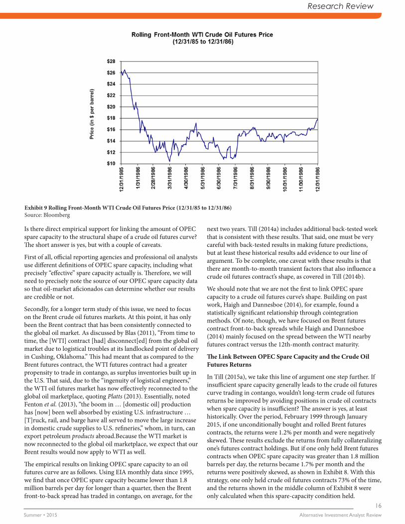
Exhibit 9 Rolling Front-Month WTI Crude Oil Futures Price (12/31/85 to 12/31/86) Source: Bloomberg

17OPEC Spare Capacity
Current Environment
As discussed in Till (2015b), spare-capacity figures have been helpful in deciding upon structural holdings in crude oil futures contracts when combined with curve-shape data. In other words, the spare-capacity situation is necessary, but not sufficient, for deciding upon whether to enter into crude-oil futures contract positions. Spare capacity has to be sufficient, but the curve shape of crude oil futures contracts also has to be supportive, ie., in backwardation.
While insufficient spare capacity has historically led to the crude oil futures curve trading in contango, this is not the only factor that can lead to a crude oil futures curve trading in contango. If there is sufficient spare capacity and ample supply, then the crude oil futures curve will also trade in contango. This is apparently the situation that we are in now: OPEC Gulf producers have shaken off their traditional role of balancing the oil market. Saudi Arabia and other Gulf oil producers had until recently acted as the central banker of the oil market and had essentially provided a free put to the marketplace in preventing a free fall in oil prices, even in the face of new oil production, particularly from the United States. Arguably, one might compare the current price environment to 1986 when Saudi Arabia and other Gulf producers apparently decided upon prioritizing market share, according to Gately (1986). Exhibit 9 shows the price path of crude oil in 1986. Drawing on Fattouh (2014), there was also ample OPEC spare capacity at the time.
How did holdings in oil futures contracts perform in 1986, both unconditionally and when using a curve-shape toggle? If one passively held and rolled WTI futures contracts, one would have lost -25.5% in 1986. Correspondingly, during that time, if one only held WTI futures contracts if the contract was backwardated, then the losses were significantly lower at -8.8%, again demonstrating the importance of curve shape as a signal.
Spare Capacity and Curve Shape
While the 1986 results may be interesting, one data point by itself is not very persuasive. In Till (2015a), we examine the historical returns of entering into crude oil futures contracts when space capacity is sufficient and when the curve shape is supportive; please see Exhibit 10.
This strategy, conditional on both ample spare capacity and the Brent futures curve trading in backwardation, is positively skewed with its worst monthly return being -15%. In this case, one only held crude oil futures contracts 45% of the time, and the returns shown in the right-hand column of Exhibit 10 were only calculated when both conditions held. When including the curve-shape toggle, the downside risk was, at least historically, further constrained, as compared to solely examining spare capacity. One could conclude that the addition of the curve toggle is advisable.
Conclusion
This article pursues the following line of logic:
(a) Over sufficiently long timeframes, it is the structural shape of a futures curve that has had a strong relationship with a commodity futures contract’s returns.
(b) What is one fundamental feature of the oil futures markets that has led to the market trading in contango? Answer: Insufficient OPEC spare capacity. Therefore, it might not be wise to enter into structural positions in crude oil futures contracts when spare capacity is at pinch-point levels.
(c) Is examining the level of spare capacity sufficient for deciding upon structural positions in the oil futures markets? The answer is no: one should also directly examine the curve shape as well.
One caveat with this article is that it analyzed the crude oil futures markets using historical data. The conclusions in the article are only useful if the states-of-the-world that occurred historically continue to be the case going forward.
Endnotes
This article is updated from the lecture, “Oil Futures Prices and OPEC’s Spare Capacity,” which, in turn, was delivered at the University of Colorado Denver Business School’s J.P. Morgan Center for Commodities on September 18, 2014 as part of the Center’s Encana Distinguished Lecture Series. (The slides for this lecture are available at: http://www.edhec-risk.com/events/other_events/Event.2014-09-02.1535/attachments/Till_JPMCC_Lecture_180914.pdf.)
The work leading to this article was jointly developed with Joseph Eagleeye of Premia Research LLC. Research assistance from both Katherine Farren, CAIA, of Premia Risk Consultancy, Inc. and Hendrik Schwarz is gratefully acknowledged.
Exhibit 10 Brent Futures (Excess) Returns, February 1999 through January 2015, with Conditional ProvisionsSource of Brent Futures Data: Bloomberg. The Bloomberg ticker used for calculating Brent Futures-Only Returns is “SPGSBRP <index>”.Source of OPEC Spare Capacity Data: EIA (2015), Table 3c.Explanation of Abbreviation: “mpd” stands for million barrels per day.Necessary Caveats: These results would only be appropriate for trading or investment purposes if (a) the EIA’s monthly data has not required substantial revisions after publication; and (b) if the state-of-the-world represented by an empirical analysis over the period, 1999-through-the-present, continues to be the case. Both assumptions cannot be guaranteed.
Conditional Solely on Previous Month’s
OPEC Space Capacity> 1.8 mbd
Brent Futures (Excess) Returns February 1999 through January
2015
Conditional on Previous Month’s
OPEC Space Capacity> 1.8 mbd AND Brent Front-to-Back Spread>0
Monthly Returns Based on Monthly Data Monthly Returns
Arithmetic Average: 1.7% Arithmetic Average: 2.0%
Skew: .42 Skew: .12
Minimum: -19% Minimum: -15%

Research Review
Alternative Investment Analyst ReviewSummer • 2015
18
References
Abu Al-Soof, N., 2007, “The Role of OPEC Spare Capacity,” Remarks at the OPEC-organized session, “The Petroleum Industry: New Realities Ahead?”, Offshore Technology Conference 2007, Houston, Texas, May 1.
Amenc, N., B. Maffei, and H. Till, “Oil Prices: The True Role of Speculation,” EDHEC-Risk Publication, November 2008. Available at:
http://faculty-research.edhec.com/research/edhec-publications/2008/oil-prices-the-true-role-of-speculation-124361.kjsp?RH=1295357717633
Arnott, R., 2014, Research Affiliates, Commodity Presentation, S&P Dow Jones Indices’ 8th Annual Commodities Seminar, London, September 11.
Blas, J., 2011, “Commodity Daily: Changing Oil Benchmarks,” Financial Times, January 11.
Büyükşahin, B., Haigh, M., Harris, J., Overdahl, J., and M. Robe, 2008, “Fundamentals, Trader Activity and Derivative Pricing,” EFA 2009 Bergen Meetings Paper, December 4. Available at: SSRN: http://ssrn.com/abstract=966692
Büyükşahin, B., 2011, “The Price of Oil: Fundamentals v Speculation and Data v Politics,” IEA Oil Market Report, Slide Presentation.
Cochrane, J., 1999, “New Facts in Finance,” Economic Perspectives, Federal Reserve Board of Chicago, Third Quarter, pp. 36–58.
[EIA] U.S. Energy Information Administration, 2014, “What Drives Crude Oil Prices?”, Presentation, Washington, D.C., January 8.
EIA, 2015, “Short-Term Energy Outlook,” January 13.
Fattouh, B., 2014, “Saudi Arabia’s Oil Policy in Uncertain Times: A Shift in Paradigm?”, Oxford Institute of Energy Studies Presentation.
Feldman, B. and H. Till, 2006, “Backwardation and Commodity Futures Performance: Evidence from Evolving Agricultural Futures Markets,” Journal of Alternative Investments, vol. 9(3), pp. 24-39.
Fenton, C., Martin, D., Speaker, S., Waxman, J., Chaturvedi, S., O’Malley, C., Hansen, M., Kabra, U. and G. Shearer, 2013, “Commodity Markets Outlook and Strategy: 2014 Outlook – And the Walls Come A-Tumblin’ Down,” J.P. Morgan Global Commodities Research, December 30.
Gately, D., 1986, “Lessons from the 1986 Oil Price Collapse,” Brookings Papers on Economic Activity, vol. 17(2), pp. 237-284.
Geman, H., 2005, Commodities and Commodity Derivatives, (Chichester: John Wiley & Sons).
Gorton, G., Hayashi, F. and G. Rouwenhorst, 2013, “The Fundamentals of Commodity Futures Returns,” Review of Finance, European Finance Association, vol. 17(1), pp. 35-105.
Gunzberg, J. and P. Kaplan, 2007, “The Long and Short of Commodity Futures Index Investing,” in H. Till and J. Eagleeye (eds) Intelligent Commodity Investing, http://www.riskbooks.com/intelligent-commodity-investing, London: Risk Books, pp. 241-274.
Haigh, M., and J. Dannesboe, 2014, “Commodities Review: Tipping Point … When Oil Markets Disconnected,” Société Générale Cross Asset Research, Commodities, June.
Harrington, K., 2005, “Crude Approximations,” Clarium Capital Management, November.
[IMF] International Monetary Fund, 2005, “Will the Oil Market Continue to be Tight?”, World Economic Outlook, Chapter IV, April, pp. 157-183.
Khan, M., 2008, “Oil Prices and the GCC: Could the Region Be Stoking Oil Prices?”, Citi Economic and Market Analysis, July 4.
McCracken, R., 2014, “The Amount of Oil the World Uses, Seen Through Different Eyes,” Platts Energy Economist, July 29.
Murti, A., B. Singer, L. Ahn, A., Panjahi, and Z. Podolsky, 2005, “Americas Energy: Oil,” Goldman Sachs, New Industry Perspective, Global Investment Research, December 12.
Nash, D., 2001, “Long-Term Investing in Commodities,” Global Pensions Quarterly, Morgan Stanley Dean Witter, January, pp. 26–31.
Nash, D., and B. Shrayer, 2005, “Investing in Commodities,” Morgan Stanley Presentation, IQPC Conference on Portfolio Diversification with Commodities, London, May 24.
Plante, M. and M. Yücel, 2011, “Did Speculation Drive Oil Prices? Market Fundamentals Suggest Otherwise,” Federal Reserve Bank of Dallas Economic Letter, vol. 6(11), October.
Platts, 2013, “Tighter Brent-WTI Spread Raises New Challenges for Refiners,” The Barrel, May 6.
Ribeiro, R., Eagles, L., and N. von Solodkoff, 2009, “Commodity Prices and Futures Positions,” J.P. Morgan Global Asset Allocation & Alternative Investment Research, December 16.
Rowland, H., 1997, “How Much Oil Inventory is Enough?”, Energy Intelligence Group, p. 7.
Till, H., 2008, “The Oil Markets: Let the Data Speak for Itself,” EDHEC-Risk Publication, October. [Ms. Till presented this paper to the International Energy Agency’s (IEA)’s Standing Group on Emergency Questions / Standing Group on the Oil Market at their joint session during a panel discussion on price formation at the IEA’s Paris headquarters on March 25th, 2009.] Available at:
http://faculty-research.edhec.com/research/edhec-publications/2008/the-oil-markets-let-the-data-speak-for-itself-122009.kjsp
Till, H., 2014a, “An Update on Empirical Relationships in the Commodity Futures Markets,” CME Group White Paper, February 28. Available at: http://www.cmegroup.com/trading/agricultural/update-on-empirical-relationships-in-commodity-futures-markets.html
Till, H., 2014b, “OPEC Spare Capacity and the Term Structure of Oil Futures Prices,” EDHEC-Risk Publication, http://www.edhec-risk.com, October.
Till, H., 2015a, “Structural Positions in Oil Futures Contracts: What are the Useful Indicators?”, Energy and Commodity Finance (ECOMFIN) Seminar, ESSEC Business School, Paris La Défense, March 27. Seminar available at: https://www.youtube.com/watch?v=i-Fg0yvcT_Q
Till, H., 2015b, “Structural Positions in Oil Futures Contracts: What are the Useful Indicators?”, Argo: New Frontiers in Practical Risk Management, a research publication of the Energy and Commodity Finance Research Center at the ESSEC Business School (France), http://energy-commodity-finance.essec.edu/research/argo-review, spring, pp. 67-81.
Working, H., 1948, “Theory of the Inverse Carrying Charge in Futures Markets,” Journal of Farm Economics 30(1), pp. 1–28.
This paper is provided for educational purposes only and should not be construed as investment advice or an offer or solicitation to buy or sell securities or other financial instruments. The views expressed in this article are the personal opinions of Hilary Till and do not necessarily reflect the views of institutions with which Ms. Till is affiliated.

19OPEC Spare Capacity
Author’s Bio
Hilary Till Co-founder Premia Research LLC,
Ms. Till is co-founder of Premia Research, LLC and the co-editor of “Intelligent Commodity Investing,” a bestseller for Risk Books and has provided presentations on the commodity markets to the U.S. Commodity
Futures Trading Commission, the International Energy Agency, and to the (then) U.K. Financial Services Authority. In addition, she has provided seminars (in Chicago) to staff from the Shanghai Futures Exchange and the China Financial Futures Exchange.
She presently serves on the North American Advisory Board of the London School of Economics; is a member of the newly formed Research Council within the J.P. Morgan Center for Commodities at the University of Colorado Denver Business School as its Solich Scholar; and is a Research Associate at the EDHEC-Risk Institute in Nice, France.
In Chicago, Ms. Till is a member of the Federal Reserve Bank of Chicago’s Working Group on Financial Markets; is an Advisory Board Member of DePaul University’s Arditti Center for Risk Management; and is a steering committee member of the Chicago chapter of CAIA.
She has a B.A. with General Honors in Statistics from the University of Chicago and an M.Sc. degree in Statistics from the London School of Economics (LSE). Ms. Till studied at the LSE under a private fellowship administered by the Fulbright Commission.
Premia Research LLC starts with the premise that all markets can become fundamentally overstretched. Accordingly, an index should either include natural hedges because of the potential of a market crash, or it should dynamically allocate out of a market during extremes in valuation. The design of the firm’s indices reflects these beliefs.

Interview with Mebane FaberMebane Faber, Chief Investment Officer, CEO, Cambria Investment Management
Featured Interview
Alternative Investment Analyst ReviewSummer • 2015
20
This summer, AIAR Content Director Barbara J. Mack had a chance to speak with serial entrepreneur and CAIA Member Mebane Faber about his career in alternative investments.
BJM: Tell us a little bit about your background and how you wound up running Cambria Investments.
MF: In college, I studied engineering and biology and after graduation I started out as a biotech equity analyst. My plan was to take a year off working before going back to get my PhD in biotech, that year quickly became a career. I never went back for the PhD, but gravitated away from biotech and towards the quant side of the investment management business, co-founding Cambria in 2006. We were managing money by 2007 through separate accounts and two hedge funds and things developed from there. The biggest initiative in the past few years has been to launch public funds through ETFs and we now have five ETFs trading and four more have been
filed and are on the way. They cover a broad spectrum, from equities to global macro to fund of funds, with both tactical and buy and hold approaches. The goal is to launch low-cost, strategy-based ETFs that everyone can access, many of which are seen as hedge fund or alternative-like strategies, but are much more tax efficient and cost effective due to the ETF structure
BJM: How did you choose the partner who launched the business with you?
MF: My partner Eric Richardson and I have complementary backgrounds – he is a lawyer and has experience in investment banking and venture capital and I was in research, so it’s nice to have his skill set, especially when we are dealing with public funds and there are a lot of regulations. You learn quickly that the business of money management is very different from managing money and you have to handle both sides effectively.

21Interview with Mebane Faber
Like many entrepreneurs, we bootstrapped the business and it took a few years to gain traction. We are known mostly for our research and publishing; I just put out our fourth book in March and have written over 1,500 articles on my blog and produced some academic articles as well. For a small company this kind of productivity has been beneficial in getting the word out and sharing our research, enabling steady growth with a small headcount.
BM: Can you give us an example from some recent research?
We try to publish research so that investors can understand our process, and hopefully, be more informed investors in our funds. As an example, in the recent book, Global Asset Allocation, we looked at about 15 of the most famous asset allocation models, including the classic 60/40 model, the permanent portfolio, and risk parity. One of the main issues that is discussed in the media and investing circles involves determining what the best allocation may be: is it the endowment model, for example? We looked at the allocations that were proposed by some of the most prominent asset managers, Rob Arnott, Ray Dalio, David Swensen, Mohammed El-Erian, and showed the results all the way back to the 1970s.
A pretty interesting take away is that a lot of the asset allocations ended up quite close to the same place, as long as you have some global stock, some global bonds, and some real assets, and the actual percentages to each category did not matter that much. What did matter a great deal were the fees paid, including the manager fees of the funds and the adviser costs. So we did a thought experiment, saying “What if you could go back to 1972 and predict the absolute best performing asset allocations in this case?” It turned out to be the endowment style portfolio, but if you executed that portfolio through an average adviser with average fees, the process would have taken the best performing “crystal ball” portfolio and transformed it into the worst one.
That is a pretty stunning revelation and so if you are working with buy and hold allocations, you should be paying as little as possible. Our research on this issue culminated in the formation of the ETF that we launched in December. We are the first company to launch an ETF with a permanent 0% management fee and it holds 29 other underlying ETFs, so all-in it only costs 0.29%, which was and may still be the lowest cost asset allocation ETF.
It comes back to the notion that investors focus so much on the allocation and particular strategies, when a lot of the “boring” parts like fees and taxes, can have a much greater impact that the actual allocation choices.
BJM: What role do the foreign markets play in your allocations?
MF: We love the foreign markets and one of the biggest mistakes that investors make is not allocating enough to foreign asset classes. If you look at the world market cap portfolio for equities, it is roughly half foreign, yet most people in the U.S. allocate around 70% to U.S. equities – this is far too much and is called home country bias.
Everything we do at Cambria is quant based, and we screen countries or foreign equities for certain characteristics that have worked well historically. These are often the same factors that work well in the U.S.: value, momentum, trend, and quality.
So we are huge believers in the international markets, especially right now, when the U.S. is one of the most expensive stock markets in the world. The good news is that the markets in most countries are attractively priced and some are really cheap, particularly in Europe, and also Russia and Brazil.
The funny thing about global market valuations is that the best places to invest are often the ones where things look the worst, geopolitically and economically. The famous Templeton quote says, Don’t ask me where things are best, that is the wrong question, ask where things are most miserable. The perfect example is Russia, last year it was in the news every day, with Putin invading Ukraine, and yet they have the best performing stock market in the world this year.
Now Greece is in the news every day – but there will be opportunities for strong returns in that market too. Their stock market is much smaller, of course, but it is a good example of a country that is very cheap now and could perform better in the future. There is another Templeton quote that might be appropriate for this situation – “Invest at the point of maximum pessimism.”
BJM: Do you think that many funds will always tend to move towards the same broad selection of assets?
MF: There is a herding effect – one of the greatest examples of this at the moment is in dividend stocks. In the late 1990s, no one wanted them in the U.S., but in looking at the factor, it was clear that dividend stocks have worked because historically they have traded at a roughly 20% discount to the overall market, based on valuation. However, in the late 1990s, that discount hit almost 50%. So that was a fat pitch – it was a great time to be investing in dividend stocks, but it was also a time when no one wanted them.
Over the next 15 years or so, the picture has changed completely. Everyone is searching for yield, and a lot of money flowed in to dividend stocks. Partly, this was the quest for yield in an environment of low interest rates; and partly this was managers and investors chasing performance. These inflows have changed the valuations of a historically attractive asset class. Not only do they not trade at a discount, they are now trading at a premium to the market. It’s not surprising that they are underperforming – because investors are choosing stocks that have yields that are comparable to the market, but with higher valuations!
You don’t have to believe me, just look at the ticker of the largest three dividend ETFs and look at their valuation metrics and it is clear that a lot of investors will be surprised by the results. There are other examples of this – low volatility strategies were a great way to invest historically, but so much money has piled in it has changed the nature of that type of investment too. In any cognitive approach, there are certain times when it works very well and certain times when it does not make sense to be investing in that strategy, at least until things change again.
BJM: The game keeps moving anyway…
MF: That’s what makes it fun and keeps it interesting!

Featured Interview
Alternative Investment Analyst ReviewSummer • 2015
22
BJM: What do you see for the near future at Cambria?
MF: We have five funds out, four funds filed and probably another six on the way. We have a number of criteria for a fund to launch. First, it has to be something I want to put my own money into – I have 100% of my net worth in these funds. Second, it has to be something that doesn’t exist, or a situation where we think we can do much better than what is out there already. Managed futures is one area that we may enter eventually, because we think the opportunities are there.
BJM: Let’s turn to CAIA – how did you discover it and what advice might you have for current candidates or members, especially those who might want to start their own firms some day?
MF: I went through the program in the early days – I must have been in one of the first few classes of the program. At that time, the curriculum was math and stats-heavy; it was focused on alternatives and also included things like insurance-dedicated funds - not what you would see in traditional financial education offerings. The designation should become even more important in the future, as we are in the seventh year of a bull market in the U.S. and stocks are expensive. This will not last forever and we will go through another cycle of recession and bear market, then alternatives will receive a lot of attention again.
For people who want to start a company, I would say, “Go for it!” I have been involved in launching three different companies – Cambria and the investment management company, Idea Farm, which is a research business, and Alpha Clone, which is a software company that also manages money and has ETFs. It is a lot of work - it can be very rewarding and very trying over time. It took three to four years to gain traction in our space; we literally started it from scratch – friends and family – and there may be easier ways to start a business and not everyone has the make-up for it. But it’s a wonderful journey and adventure and we have plenty more ideas for the future.
Author’s Bio
Mebane Faber, Chief Investment Officer, CEO Cambria Investment Management
Mr. Faber is a co-founder and the Chief Investment Officer of Cambria Investment Management. Faber is the manager of Cambria’s ETFs, separate accounts and private investment funds. Mr. Faber has authored
numerous white papers and three books: Shareholder Yield, The Ivy Portfolio, and Global Value. He is a frequent speaker and writer on investment strategies and has been featured in Barron’s, The New York Times, and The New Yorker. Mr. Faber graduated from the University of Virginia with a double major in Engineering Science and Biology.

The Time Has Come for Standardized Total Cost Disclosure for Private EquityAndrea Dang, CFA Senior Analyst CEM Benchmarking, Inc.
Mike Heale, MBA Principal CEM Benchmarking, Inc.
David Dupont, CFA Senior Analyst CEM Benchmarking, Inc.
News and Views
23Standardized Total Cost Disclosure for Private Equity
Given the level of detail and timing of private equity manager reports, can pension funds disclose investment costs in a consistent manner across the industry? What would full cost disclosure require of a pension fund? We found a good example of this in one of our benchmarking clients.
In 2013, the South Carolina Retirement System Investment Commission (SCRSIC) retained CEM Benchmarking Inc. (CEM)1 to perform an independent review of South Carolina Retirement Systems’ (South Carolina) investment costs and performance. SCRSIC naturally assumed that the costs benchmarked by CEM would match the investment costs that are reported in South Carolina’s Comprehensive Annual Financial Report (CAFR). To their surprise, CEM could only benchmark about 50% of the investment costs reported in South Carolina’s CAFR.
South Carolina invests more assets in alternative investments, such as private equity (PE), hedge funds and real estate, than many other U.S. public funds. Their allocation to alternatives of 30% as per their 2014 CAFR [1] compared to the CEM U.S. public universe average of 19% in 2013. Alternative asset classes, especially private equity, are typically more expensive and have more complex cost structures than public asset classes. This makes cost disclosure and cost benchmarking difficult at best. For the portion of costs that CEM can now benchmark for U.S. funds, CEM’s analysis found that South Carolina’s investment costs were in line with those of other public pension funds after adjusting for fund size and asset mix.
South Carolina’s CAFR generated some negative press coverage that alleged their investment costs were unjustifiably high. However, after reviewing SCRSIC’s cost collection process, we conclude that they are simply reporting more costs than other funds, rather than

News and Views
Alternative Investment Analyst ReviewSummer • 2015
24
actually incurring more costs. CEM authored this paper to create momentum for improving investment cost reporting standards and disclosure, especially for private equity. Less than one-half of the very substantial PE costs incurred by U.S. pension funds are currently being disclosed.
U.S. Reporting Standards Allow Public Funds To Exclude Material Costs
To better understand this problem, we first examine accounting standards and practices for pension fund cost disclosure. State pension funds follow the Governmental Accounting Standards Series issued by GASB. Until recently, all state pension funds were subject to Statement No. 25 [2] from November 1994, which sets standards for financial reporting for defined benefit pension plans. Paragraph 29, footnote 12 states the following:
“Plans are not required to include in the reported amount of investment expense those investment-related costs that are not readily separable from (a) investment income (the income is reported net of related expenses) or (b) the general administrative expenses of the plan.”
This footnote is ambiguous and permits a widely varying interpretation of what investment costs are “readily separable” from investment income and general administrative expenses of the plan.
In June 2012, GASB issued Statement No. 67 [3], which is an amendment to Statement No. 25. Paragraph 26 of Statement No. 67 states the following:
“Investment-related costs should be reported as investment expense if they are separable from (a) investment income and (b) the administrative expense of the pension plan.”
Statement No. 67 makes two subtle changes in language from Statement No. 25:
• Statement No. 25 indicates that disclosing certain investment-related costs is not required, while Statement No. 67 makes no explicit mention of allowance for exclusions.
•The phrase “readily separable” is no longer present in Statement No. 67.
Statement No. 67 leaves it up to funds to interpret what costs are separable. This remaining ambiguity still allows very material costs that are netted from returns to be excluded from financial statements. In practice, the amended guidelines have not led to more transparent cost disclosure, especially for PE.
Private Equity Cost Structures Are Complex And Reporting Is Incomplete
Pension funds typically invest in private equity via limited partnership structures managed by a PE firm, the general partner (GP). Costs incurred by limited partners (LPs) (i.e., revenues to the GP) include a management fee, carried interest or performance fees, other fund-level fees, and portfolio company fees. Fund of funds structures include an additional layer of fees paid to the GP choosing the underlying investments. LPs also incur their own internal costs for monitoring of their external PE program.
Carried interest is typically based on gains above a preferred return over the life of the investment. Because the gains are not yet fully realized before the end of the investment life, carried interest will vary and is not easily calculated. Frequently, the LP’s share of carried interest is not clearly disclosed on interim statements. However, accrued carried interest is commonly netted from returns.
Other fund-level fees include fees paid by the GP that are passed onto LPs. Examples include legal costs, audit costs, and taxes. Other fund-level fees are also often not reported in detail to LPs quarterly.
Portfolio company fees are paid by the portfolio company to the GP for advisory services, break-up, monitoring, funding, and similar services. Portfolio company fees shift dollars from portfolio companies to the GP, lowering future returns for LPs. The LP is typically entitled to a portion of portfolio company fees, which is commonly referred to by the industry as a management fee rebate or offset. Often, the LP share is not explicitly transferred, but is kept by the GP and used as payment towards a portion of the management fee. The residual fee amount, which is the full management fee less the LP share of portfolio company fees, is described as the net management fee. Only this amount is typically disclosed to LPs on capital call statements.
We believe that the LP share of portfolio company fees is misrepresented by the industry as a management fee rebate or offset. The net management fee amount does not reflect total management fees paid to the GP because the “rebated” amount is still an expense to the portfolio company and therefore an indirect cost to the LP. LPs actually pay the full management fee, and the portion of portfolio company fees kept by the GP is an additional cost. In other words, the fee rebate or offset gives the illusion of reduced fees for the LP when, in fact, it is a charge to the portfolio company. And, when the offset is not 100% for the LP, the un-rebated percentage has the effect of increasing GP overall revenue. Typically, only the net management fee is reported by pension funds.
Exhibit 1 shows an illustrative example of the relationships between full management fees, net management fees, and portfolio company fees.
Unfortunately, due to the difficulty of collecting all cost components and the lack of standardized cost definitions, many funds are unable to report full PE cost. As can be seen in Exhibit 2, very material costs are not being reported.
Exhibit 2 shows that carried interest, other fund-level fees, and portfolio company fees represent more than half of total PE cost. Public pension funds that do not report these costs are excluding substantial amounts. For a $3 billion PE portfolio, the average difference between what funds actually report and the estimated total PE cost is 202 basis points or $61 million.
PE fund of fund structures introduce additional layers of costs that include management fees and performance fees paid to the top-level manager. For our Dutch clients in 2012 and 2013, total PE fund of fund costs were 5.04%.2 This means that fund of fund investors on average paid 1.22% more than direct LP investors due to these additional costs.

25Standardized Total Cost Disclosure for Private Equity
The U.S. Securities And Exchange Commission (SEC) Has Drawn Attention To PE Firms’ Lack Of Cost Disclosure
In October 2012, the SEC’s Office of Compliance Inspections and Examinations (OCIE) began conducting presence exams on PE firms as a result of the Dodd-Frank Act. In May 2014, OCIE released its results of the presence exams [4], which included findings on PE fees and expenses. OCIE found violations or material weaknesses relating to expenses paid for advisory services in more than half the examinations. Specifically, the adviser fees were paid by portfolio companies or the PE fund but were not sufficiently disclosed to LPs. OCIE also found instances of hidden fees such as accelerated monitoring fees, undisclosed administration fees not covered by the limited partnership agreements (LPA), excessive transaction fees beyond the limits set in the LPA, and fees paid to third-party advisers who did not adequately deliver their services.
Given the issues the SEC has uncovered, LPs should be concerned regarding the lack of transparency for PE costs. OCIE noted that while extensive due diligence is usually performed prior to investing, oversight during the life of the fund is not as rigorous. It is prudent for investors in a fiduciary role to proactively attempt to identify and disclose all fees paid for PE. This would help fiduciaries fully understand their PE fee structures, recognize how their PE costs compare to similar investors, and provide their stakeholders with needed transparency. However, for this to be achieved, standardized manager reporting is required. Mounting interest in verifying these costs from both the SEC and pension funds could move the industry towards improving and standardizing private equity cost disclosure.
South Carolina Has Developed An Extensive And Rigorous Process For Identifying And Reporting Private Equity Costs
As part of its cost validation process, SCRSIC makes a good faith effort to collect, check for reasonableness, and report full investment costs. They report net management fees, carried interest, and other fund-level expenses in the plan’s CAFR.
The CAFR Schedule of Investment Managers and Fees shows two categories of fees – manager fees that were directly invoiced and manager fees that were deducted on a net-of-fee basis. The category of manager fees that were deducted on a net-of-fee basis is SCRSIC’s best attempt to report fees that were netted from net asset value (NAV) and not readily separable. For comparison, fiscal year 2014 invoiced fees represented only about 8% of their total reported investment fees, which means all other costs were netted.
SCRSIC uses a detailed validation process that has been especially useful for capturing and disclosing PE costs during their fiscal year. SCRSIC has found that they cannot collect total investment costs using only manager statements due to timing and a lack of consistency. Managers’ annual reports for PE are usually based on a calendar year, while South Carolina has a June 30 fiscal year end. And, the unaudited quarterly PE statements are not consistent across managers in their detail and/or depth of fee disclosure.
To correct the timing issue, the validation process is performed on a quarterly basis. SCRSIC provides a detailed capital account statement template for their PE managers to fill-out each quarter. The expenses portion of the template includes lines on which to
Exhibit 1 Illustrative example of management fees and portfolio company fees Source: Author’s calculations
Exhibit 2 Private equity estimated full costs and reported management fees Source: CEM Universe, 2012-2013
Full management fees Portfolio company fees
165 basis points (bps) 50 bps
Assuming that the general partner is entitled to 20% of the portfolio company fees:
General partner receives 10 bps.
Limited partner receives 40 bps.
Typically reported management fees = Full management fees - LP share of portfolio company fees = Net management fees = 165 bps - 40 bps = 125 bps
Actual costs incurred by LP = Full management fees + GP share of portfolio company fees = 165 bps + 10 bps = 175 bps
(CEM Universe, 2012-2013)Median annual cost based
on net asset valueCost in $ millions based on
a $3 BN portfolioFull management fees2 1.89% $56.7Internal monitoring costs2 0.08% $2.4Carry/performance fees2 1.49% $44.7Other fund-level and portfolio company fees 0.36% $10.8Estimated total direct LP costs3 (A) 3.82% $114.6Reported management fees4 (B) 1.80% $54.0Difference (A-B) 2.02% 60.6

News and Views
Alternative Investment Analyst ReviewSummer • 2015
26
report full management fees, the LP share of portfolio company fees which is used towards payment of the management fees, other fund-level fees, and accrued carry/performance fees that are deducted from NAV for the period. The capital account statement format ensures that the manager reconciles the costs associated with the change in NAV for the period. This provides SCRSIC with a first level of quality control for reported fee data. Based on other provided data such as contributions, invested value, and distributions, the expected full management fee and performance fee are compared to the partnership contract terms. SCRSIC reconciles their manual calculations from the contract terms to the fee amounts provided by the managers. If there are material discrepancies, SCRSIC asks for explanations and documents the changes for future validations.
While the vast majority of managers comply with the SCRSIC process, a few managers do not complete the template. For those accounts, SCRSIC manually collects data from statements that are provided and asks for any missing figures. Since this process is more manual, it is more time-consuming.
The ability to collect and confirm reasonableness of cost data from PE managers relies on a strong understanding of the partnership contract terms and constant communication with managers. As a result, implementing such a validation process requires resources. While SCRSIC has found that most of their managers are willing to complete the template, the main challenge is ensuring that all managers provide consistent data with formats and time periods that are specific to their validation process.
This extensive validation process that attempts to capture total investment costs demonstrates the point of this document: the need for standardization.
Since 2009, the Institutional Limited Partners Association (ILPA) has been developing private equity best practices and standardized reporting templates that emphasize providing transparency to LPs. Their templates are robust and include detailed investment fees and expense information. However, the best practices and templates are not mandatory standards enforced by a governing body and generally the industry has not adopted these to date.
Many pension funds do not undertake a detailed validation process perhaps because it is very manual and they may not have enough resources. SCRSIC has discussed cost reporting with other funds. They have found that funds implement different methods for cost reporting. For example, one fund told SCRSIC that they take a “report as it is reported approach,” which means only explicitly disclosed or invoiced costs are reported. Given this view, it is not surprising that South Carolina’s reported investment costs are higher than other funds.
Some Countries Require More Transparent Cost Disclosures
In the Netherlands, the Federation of Dutch Pension Funds introduced new reporting standards in 2012 [5] requiring Dutch pension funds to show full investment costs. These standards have been adopted by the Dutch central bank, De Nederlandsche Bank (DNB), with the expectation that all Dutch pension funds will comply with their 2014 financial statements. Specifically for PE, full investment costs include full management fees, performance fees, consulting fees, monitoring fees, and transaction costs.
Similar investment cost reporting standards have also been implemented recently in Denmark and Switzerland. Both countries’ reporting standards have a stand-alone section or document devoted specifically to PE costs. Under these new reporting standards, the components of PE cost are explicitly defined and include management fees and performance fees as well as administration and transaction costs.
Cost Disclosure And Transparency Can Lead To Better Decisions
Clearly there currently are challenges with collecting full PE costs, but the exercise can yield benefits beyond improved disclosure and transparency. Understanding true costs can lead to lower costs through negotiation with managers. For example, greater understanding of portfolio company fees has led to a big change in the proportion of portfolio company fees distributed to LPs. Over time, this revenue sharing has shifted from a 0%/100% LP/GP split to an average closer to 85%/15%5 today.
Additionally, understanding costs may lead to more efficient investment vehicle selection because high costs will materially impact PE performance. Exhibit 3 shows the net returns and value added for different implementation styles. Fund of funds underperformed internal investing by more than 5% and direct LPs underperformed internal by more than 3%.
Cost disclosure is the main focus of this paper. But costs are neither inherently good nor bad and should not be considered in isolation. Higher costs are justified if they produce higher returns. PE has been a strong performing asset class for some pension funds. For other funds the opposite is true – net PE returns have substantially underperformed public equity market benchmarks. CEM believes that the main performance differentiator between the two groups is implementation costs. Where costs are very high, performance suffers in lock step. PE fund of fund total cost averaged 5.04%. Net value added was 5.15% lower than low cost internal PE implementation. To maximize value creation, funds need to understand the impact of full costs on their decisions.
Exhibit 3 Average annualized compound private equity net performance7
Source: CEM Universe, 1996-2012
(CEM Universe, 2012-2013)Internal Direct LP Fund of funds
Annualized net return 12.21% 9.64% 7.15%Annualized benchmark return6 8.69% 9.36% 8.77%Net value added 3.52% 0.28% -1.63%

27Standardized Total Cost Disclosure for Private Equity
When asked to comment on their current fee reporting practices, Michael Hitchcock, Executive Director of South Carolina Retirement System Investment Commission, responded, “RSIC believes that part of our duty to stakeholders and policy makers is the most complete fee transparency we can achieve. We are pleased to be a leader in this field, and we hope that our practices along with other plans’ needs in this area help move the industry towards improving and standardizing private equity fee disclosure.”
And momentum is building towards greater cost disclosure around the world. Christopher Ailman, CIO of California State Teachers’ Retirement System, recently vocalized the need for cost reporting standards, especially within the alternatives space. As stated by Mr. Ailman, “We need someone to propose an industry standard, once posted everyone in the industry debates and then you issue a standard. And it becomes something we need to follow.” [7]
CEM agrees with Mr. Ailman and we want to work with pension funds and interested parties to make this happen. With the support of the pension fund industry, we can make great strides in improving private equity cost reporting.
Endnotes
1. CEM is an independent global benchmarking and research organization located in Toronto, Canada, that has provided investment and administration benchmarking and research services to large pools of capital (including defined benefit and defined contribution pension plans, endowments, and sovereign wealth funds) since 1991. The CEM databases contain performance and cost information from more than 1,000 pension and sovereign wealth funds from around the world.
2. Data were provided by 29 Dutch funds in 2012 and 34 Dutch funds in 2013. Dutch private equity costs are representative of full costs since the Federation of Dutch Pension Funds developed full-cost disclosure guidelines effective 2012. Costs may be understated; not all funds have adapted to the new disclosure guidelines and an estimate is used for those funds.
3. Total shown is the sum of the median cost for each cost type.
4. Reported management fees are the fees provided by non-Dutch funds in the CEM universe for 2012 and 2013.
5. CEM collected limited partnership details, including the LP share of portfolio company fees, from funds that were able to provide this information for the 2013 data year.
6. CEM developed customized private equity benchmarks based on lagged, small-cap equity indices.
7. Adapted from “How Implementation Style and Costs Affect Private Equity Performance” by Alex Beath, Chris Flynn and Jody MacIntosh, 2014, Rotman International Journal of Pension Management [6]
References
[1] South Carolina Public Employee Benefit Authority, “South Carolina Retirement Systems Comprehensive Annual Financial Report For the Fiscal Year Ended June 30, 2014,” December 2014.
[2] Governmental Accounting Standards Board, “Statement No. 25 of the Governmental Accounting Standards Board,” No. 116-A, November 1994.
[3] Governmental Accounting Standards Board, “Statement No. 67 of the Governmental Accounting Standards Board,” No. 327-B, June 2012.
[4] Bowden, A. J., “Spreading Sunshine in Private Equity,” Private Equity International, Private Fund Compliance Forum 2014, New York, NY, May 6, 2014. Available at U.S. Securities and Exchange Commission website: http://www.sec.gov/News/Speech/Detail/Speech/1370541735361#.VLl7mSvF9yw
[5] Federation of the Dutch Pension Funds, “Recommendations on administrative costs – Further elaboration on asset management costs,” November 20, 2012.
[6] Beath, A. D., Flynn, C., and MacIntosh, J., “How Implementation Style and Costs Affect Private Equity Performance, Journal of International Pension Management,” Vol. 7 Issue 1, Spring 2014. Available at SSRN: http://papers.ssrn.com/sol3/papers.cfm?abstract_id=2449784.
[7] Personal communication, March 5, 2015.

News and Views
Alternative Investment Analyst ReviewSummer • 2015
28
Authors’ Bios
Andrea Dang, CFA Senior Analyst, CEM Benchmarking Inc.
Andrea is a part of the Investment Benchmarking team that is responsible for producing the CEM Global Investment Benchmarking reports for defined benefit and defined contribution clients. As a Senior Analyst, she works with clients to
ensure data quality is high and develops reporting solutions to meet client needs.
Prior to joining CEM in 2013, Andrea worked at Mercer in the Investment Consulting group, specializing in defined benefit pension fund investment structure, asset-liability management and performance monitoring. Andrea holds a Bachelor of Mathematics degree in Mathematics & Business Administration from the University of Waterloo.
Mike Heale, MBA Principal, CEM Benchmarking Inc.
Mike oversees global business development and client service for CEM’s pension investment and administration benchmarking businesses. His personal clients include leading pension funds in Africa, Asia, Europe, the Gulf, and the United
States. Mike is a frequent speaker at pension conferences and events around the world.
Prior to joining CEM in 1999, Mike had 12 years of pension and life insurance marketing experience. He started his career in education as a basketball coach and lecturer at Laurentian University. Mike has an undergraduate degree in Physical and Health Education from Laurentian and a Master of Business Administration degree from the Richard Ivey School of Business, University of Western Ontario.
David Dupont, CFA Senior Analyst, CEM Benchmarking Inc.
David is a Senior Analyst for CEM’s Investment Benchmarking service and works on various client reporting for both defined benefit and defined contribution plans. Prior to joining CEM in 2006, David worked at CIBC Mellon for eight years in a variety of departments ranging from pension accounting to sales and marketing. David is a CFA charter holder and has a degree in Mathematics and Philosophy from the University of Toronto.

The Hierarchy of AlphaChristopher M. Schelling, CAIA Director of Private Equity Texas Municipal Retirement System
CAIA Member Contribution
29The Hierarchy of Alpha
“Skeptical scrutiny is the means, in both science and religion, by which deep thoughts can be winnowed from deep nonsense.” - Carl Sagan
Hedge funds and private equity funds have had their share of detractors over the last few years, with many institutional investors questioning whether the returns they have generated justify the significantly higher fees paid. Certainly, on a relative performance basis, a large number of these funds have had a tough time keeping up with long-only equities. Since January of 2009, the S&P 500 total return index has nearly tripled, generating annualized returns around 18%. No one should expect alternatives to match this blistering pace over any time period.
There is also no debate that alternatives have become a much more competitive sector. Hedge funds and private equity funds alike now boast 8,000 to 10,000 active funds managing $3 to $3.5 trillion dollars respectively, each roughly doubling in size since 2006 as institutional investors have piled into the space en masse.
Such growth simply cannot come without both lower quality entrants attracted to the business opportunity and the inexorable erosion of returns from larger quantities of capital chasing the same alpha strategies. Perhaps then institutional investors should not be surprised to see the return of median managers lower than in the past.
Certainly, negotiating lower fees is one way to mitigate the effect of a falling median, but successfully building a portfolio of hedge funds or private equity funds today requires more than this. For those investors continuing to pursue such strategies, success as always is likely to revolve around selection of top quartile managers. However, given the dynamics described above, the elusive search for alpha has become harder, as the costs associated with being average have gone up along with the resources needed to scour an increasingly large universe of managers. In effect, the needle has gotten smaller and the haystack has gotten bigger.

CAIA Member Contribution
Alternative Investment Analyst ReviewSummer • 2015
30
While some institutional investors have responded to these challenges by simply winding down their allocations to hedge funds and private equity funds altogether, it appears the far larger majority have not. Hedge funds continue to attract positive flows month after month, and nearly 2,000 private equity products are currently in active fund raising, according to Preqin.
Demand remains strong for these return streams, but investors continuing the search for alpha often face heightened skepticism around both the presence of true alpha and an allocator’s ability to identify it. Of utmost importance here is the realization that not all alpha is created equal. The concept of a clean, binary separation between alpha and beta, although intuitively appealing, is far too simple a paradigm for the complex realities of active investing. Like many purely mathematical approaches, it fails to capture the areas of gray. Alpha to beta is a spectrum, and often what once was the former eventually becomes the latter.
This skeptical scrutiny around the presence of what I’ll call “true alpha” seeks a better framework for the classification of investment skill. This classification mechanism should not only describe the nature and source of the return stream, identifying the manager’s ability to access this return and the probability of it continuing in the future. But even more importantly, the framework should present investment skill as a spectrum. The endpoints of the spectrum merely provide the beginning of the analysis, not the end.
I propose such a framework below.
The rarest investment skill is that which is structured with no known correlations to other returns. Such a skill would be
difficult to find, and highly expensive if one could identify it. Few managers could offer truly competing products. On the other hand, the most common return stream would be one that was highly price competitive, with thousands of managers providing nearly identical products. Still investment skill, but clearly far less valuable.
Fortunately, the argument for hedge funds or private equity does not rest on the head of a pin, or the top of a pyramid as it were. Instead, most managers in these sectors are structuring return streams that fall somewhere in between. Understanding the skill required to generate these returns is critical to manager selection.
True alpha is generally what most market participants mean when they are referring to “alpha.” This is superior skill, or outperformance resulting solely from the active selection of securities that differ from the market. This kind of alpha is truly beating the market, or outsmarting the competition, without embedded style tilts. For instance, stock pickers who do not take value, dividend, growth, capitalization, or sector bets, but still generate excess returns are generating true alpha. This form of alpha, the purest form, is also the rarest. Managers that generate sustainable, repeatable true alpha are few and far between, likely only a handful at any given time. True alpha is harder to underwrite with confidence, precisely because it so rare. A much larger sample set is required to ensure that what appears to be alpha is not merely a misidentified beta or, worse, mere luck.
Manufactured alpha can also be thought of as value creation. Security selection, although not unimportant, is not the main driver of excess return in this category. Unlike pure passive
True Alpha
Manufactured Alpha
Inaccessible Risk Premium
Pure Beta
Exhibit 1 Hierarchy of Investment Skill

31The Hierarchy of Alpha
investment, manufactured alpha requires an investor to initiate an investment with a view to impart structural changes or operational improvements that will unlock or actually create value and then ultimately execute on that vision. This usually involves repositioning the asset for resale to another buyer with a different cost of capital, similar to transitional alpha, as we’ll see below, but only after some actual value enhancement from the asset owner. For example, Re-REMICS, shareholder activism, mortgage servicing rights and re-performing loans, private equity turnarounds, and value added real estate are examples of this category of alpha generation. Given the operational, process-oriented nature of these strategies, managers who have executed successfully on them in past tend to demonstrate strong persistence of performance in the future.
Transitional alpha is the excess return that can be generated from short-term changes or specific temporal market inefficiencies. Often times, these inefficiencies result from regulatory changes, for example Basel III and the Volcker Rule, or other socio-political events which alter previous market dynamics. Other times, economic changes or even technological shifts can change the cost of capital or utility functions of market participants, which impacts their ability to transact in a given marketplace. Even other times, such transitional alpha can simply occur from shifting levels of risk aversion or changing investment fads. Think of these situations as events where typical, natural holders of a given security are structurally prohibited from transacting as easily as in the past. Several examples of these opportunities include regulatory capital relief trades, spin-offs or post-reorg equities, niche direct origination strategies where traditional lenders have exited, or even to a certain extent simply downgraded high yield bonds. In such situations, somewhat shorter term, ephemeral circumstances cause forced selling from current holders and/or remove natural buyers from the supply-demand equation. In short, transitional alpha can be generated from holding certain
assets until such time as natural buyers can come back into the equation and prices normalize. One may consider this a form of alpha, as the temporary nature of the inefficiency requires active, sometimes rapid, analysis and execution in order to capture the opportunity. Often, it is difficult for an end allocator to assess the opportunity set before it is gone, making a manager’s ability to identify and shift from one transitional investment to another key.
An inaccessible risk premium may not be alpha in the truest sense of the word, but this category logically sits between transitional alpha and alternative beta. Similar to transitional alpha, an inaccessible risk premium can exist where structural forces prevent many market participants from investing in specific investment segments. However, unlike the short-term, temporary nature of transitional alpha, an inaccessible risk premium is quasi-permanent in nature. For example, safe harbor exemptions to the 1940 Investment Company Act effectively preclude private investment companies from accepting retail investors. Sometimes, investors are unable to allocate to illiquid investments due to short-term cash flow needs or investment minimums. Retail investors simply cannot invest $5,000 directly in a privately negotiated commercial mortgage. In other circumstances, certain investors are prohibited from using derivatives or have significantly higher costs of leverage than other market participants due to suitability requirements or exchange rules. Some investors, such as some state pensions, are actually precluded by law from using leverage at all. As mentioned, these type of structural constraints tend to be long-term in nature and widely known. Not much analysis or timely response is needed to interpret and asses their affects. However, these inaccessible risk premiums have barriers to entry that require some active management in order to access, making them, if perhaps not actual alpha, something other than a simple beta. Given the structural nature of the opportunity, these investments tend to be somewhat easier to underwrite with confidence.
True Alpha
Manufactured Alpha
Inaccess ible Risk Premium
Pure Beta
Exhibit 2 Evolution of Investment Skill

CAIA Member Contribution
Alternative Investment Analyst ReviewSummer • 2015
32
An alternative beta is axiomatically no longer alpha, nor is it however a pure beta. Alternative betas are investment opportunities that at one point may have been one of the above categories of alpha, but have become more accessible and more broadly understood. Often these opportunities have liquid, registered products which allow access to a much wider array of potential investors. Such products create relatively low fee, low minimum, investable and benchmark-able return streams similar to pure betas. Unlike pure betas, alternative betas are less widely researched, less widely championed, and subsequently less widely adopted in investor portfolios. Examples of alternative betas could be catastrophe bonds, merger arbitrage mutual funds, long only commodities, currency carry ETFs, and mechanical trend following products. These return streams simply have shorter track records and fewer adherents, at least for the time being, than do the completely ubiquitous pure betas.
Finally, pure betas are quite simply basic asset class exposures that have been around for a long time. Pure betas have decades of price history and extensive research that is widely available. These betas are broadly, perhaps universally, accepted as the basic building blocks of portfolios. Pure betas are usually offered via thousands of competing low-fee products, as opposed to sometimes just a few, as is the case for many alternative betas. Pure betas are available to investors of any experience level or asset size. In short, pure betas are entirely commoditized return streams.
It’s worth mentioning that these categories of investment skill are themselves spectrums rather than discrete individual classes. Fundamental indices and smart beta products fit neatly in this hierarchy, although it’s debatable whether they fall more towards the alternative beta or pure beta side. The point is, such strategies take advantage of factors that are widely known, quite commonly employed and offered across numerous similar, if not identical, easily accessible competing products.
This framework of investment skill can also provide insight into prioritization of due diligence efforts for manager selection professionals. For example, investment opportunities that fall nearer to the top of the spectrum require more attention on the skills, abilities, and experience of the people making risk decisions. As the strategy becomes more institutional and more widely adopted, due diligence efforts should focus on the investment process itself, such as how ideas are generated and technical aspects of portfolio construction. Finally, once a strategy gains even more adherents, commoditized factors such as fees are increasingly relevant.
Interestingly, this parallels the migration or evolution of investment skill from alpha to beta. A select few individuals adept at pattern recognition are able access an investment strategy initially. The process becomes systematized, institutionalized, and others internally and externally begin to learn the strategy and are able to replicate it. As other market participants implement it and often academics write about it, the strategy eventually becomes more widely implemented and ultimately turns to beta, whereby relative performance and costs are dominant considerations when hiring a manager.
In order to underwrite some expected level of alpha for an investment in a hedge fund, private equity fund, or any investment product, an allocator must truly understand the source, scope, and nature of that alpha, or more fundamentally, whether or not it is truly alpha. Historical performance analysis plays a role in this, but like any analysis of data, the best it can do is merely provide evidence of a relationship. A comprehensive qualitative framework that focuses the process on determining exactly why and how a manager generated past excess returns is helpful in establishing a descriptive, theoretical foundation for why that relationship may have existed. Only then can an investor turn to what the competitive dynamic in that particular market currently is, what might be reasonable expectations for future returns, and finally accurately price those return streams.
A heaping dose of skeptical scrutiny, a scientific approach to evaluation, and a clear theoretical framework can be helpful towards the task of winnowing true alpha from the deep nonsense of short- term performance noise, luck, and the never-ending pitches of high-energy salesmen.
Author’s Bio
Christopher M. Schelling, CAIA Director of Private Equity, Texas Municipal Retirement System
Christopher is currently the Director of Private Equity at the $24 billion Texas Municipal Retirement System. In this role, Mr. Schelling is responsible for all aspects of building out the system’s private equity portfolio. Previously, Mr.
Schelling was the Deputy CIO and Director of Absolute Return for Kentucky Retirement Systems where he implemented the plan’s first direct allocations to hedge funds and real asset funds. Mr. Schelling was also an Adjunct Professor at the Gatton School of Business at the University of Kentucky, lecturing on Alternative Investments. Prior to joining KRS in 2011, he was a Senior Associate at Mercer Investment Consulting on the manager research team performing due diligence across hedge fund strategies. Previously, he served in a number of front and middle office roles spanning traditional and alternative investments at firms such as ThomsonReuters, Bear Stearns, and Calamos Investments.
In addition to being a member of the CAIA Association, Mr. Schelling has also served on the association’s Due Diligence and Regulation Curriculum Committee and the Exam Council. He received an MBA from the University of Illinois-Chicago and a Masters Degree in Financial Markets from the Illinois Institute of Technology. He holds a Bachelor’s Degree in Psychology from the University of Illinois as well. Mr. Schelling was named one of Money Management Intelligence’s 2012 Rising Stars of Public Funds, and a Rising Star of Hedge Funds by Institutional Investor in 2014.

Private Market Real Estate Investment Options for Defined Contribution Plans: New and Improved SolutionsCatherine Polleys Partner Aon Hewitt Investment Consulting, Inc.
Jani Venter Senior Consultant Aon Hewitt Investment Consulting, Inc.
Investment Strategies
33Private Market Real Estate Investment Options for Defined Contribution Plans
Why Incorporate a Private Real Estate Investment Option into a DC Plan?
Defined Contribution plans are rapidly becoming one of the primary retirement saving vehicles for Americans.1 Historically, DC participants have had minimal exposure to private real estate holdings due to a lack of viable investment options and concerns regarding private real estate’s potential illiquidity, historical valuation policies, and pricing frequency. As a result, if DC Plans have exposure to real estate today, it mainly consists of a small allocation to publicly-traded Real Estate Investment Trusts (REITs). Notably, only 26%2 of DC participants today have the option to invest in real estate, with overall portfolio allocations averaging only 1%,3 mostly through REITs as stand-alone investment products. In contrast, the majority of Defined Benefit (DB) plans have exposure to real estate and allocations average 8.9%,4 with over 85% of this allocation in private real estate.
REITs represent one segment of the real estate asset class, and while they exhibit long-term correlation with private core real estate, REITs have a different risk/return profile and are often used to play a different role in portfolio construction. While both vehicles provide real estate sector exposure, private real estate vehicles provide investors with direct access to the diversifying market and income characteristics of the underlying bricks-and-mortar real estate. They do this without complications from potential financial engineering, business enterprise value, and overall broader equity market volatility that are present in REITs.
The characteristics driving the differences between private and public real estate are as follows:
The daily-valued private market real estate vehicles available to DC plan sponsors are investment funds that substantially invest in core real estate

Investment Strategies
Alternative Investment Analyst ReviewSummer • 2015
34
assets that are typically well diversified by property type and geography and use modest levels of leverage. Core real estate is generally defined as a set of stabilized (well-leased), income-producing assets most commonly garnered in apartments, retail, industrial, and office property types.
REITs are operating companies and thus offer shares in a company that owns and manages the real estate assets. REITs can trade at substantial premiums or discounts to the underlying real estate values based on non-real estate and broader stock market sentiments, creating a different return profile and offering less of the diversification benefits of investing in private core real estate.
These structural and tactical differences lead private and public real estate to perform differently over a market cycle and provide different benefits, as well as challenges, when added to an investment portfolio.
The Benefits of Private Core Real Estate
The primary inclusion objective for real estate within a DC plan should focus on obtaining income and diversification, with some potential for inflation hedging over multi-year investment horizons. These goals are best met within the real estate asset class by incorporating private core real estate into a multi-asset class portfolio. The key benefits of adding private core real estate are as follows:
Attractive yields and risk-adjusted returns
Diversification and increased downside protection, and
Potential for inflation protection without increased volatility
Returns: A large portion (approximately 2/3rds) of private core real estate returns comes from cash flows generated by long-term leases that contribute to a more stable overall return profile compared to equities. Over the past 20 years,5 U.S. private real estate’s cash yield as measured by the NPI produced an annual average return of 5.1%.6 Private real estate also provides an attractive absolute return profile with significantly lower volatility when compared to equities over the same time period. Therefore, adding private real estate to a multi-asset class portfolio supports an improved overall risk/return profile for the total portfolio.
Diversification: Given private core real estate’s low correlation with equities and its relatively stable and high cash yield, the segment’s total return is less likely to be negative at the same time as equities, providing significant total portfolio benefits when adding private real estate to a multi-asset class portfolio. Given that the inclusion of private real estate is done with an eye to mitigating downside risk, we examine how often in the same-period private core real estate7 experienced negative returns when compared to a standard 60/40 stock/bond portfolio.
Over a 20-year time period, the returns for private core real estate yielded negative returns at the same time as a 60/40 stock/bond portfolio in only 14%8 of the quarters. In comparison, due to REITs’ public format, especially now that many large REITs are included in major stock indices including the S&P 500, REITs experienced negative returns at the same time as a 60/40 stock/bond portfolio in 57% of quarters.
Inflation: Both private and public real estate offer potential inflation protection over the long term. While neither provides a perfect inflation hedge, a rise in inflation over time is generally at least partially offset by rising commercial rents and the pass-through of expenses to tenants, creating the potential to hedge inflation over the medium- to long-term. Private real estate’s return profile is less volatile than other publicly-traded, inflation-sensitive assets – such as REITs, commodities, and infrastructure stocks – and this allows investors to add private real estate to their investment portfolios in scale without increasing overall portfolio volatility.
As an example, if a plan with a 60/40 stock/bond portfolio had added a 7%9 allocation to private real estate over the past 20-year time period, the real estate returns would have decreased the portfolio’s overall volatility by 60 bps.10.
In comparison, a 7% allocation to REITs would have increased the portfolio’s overall volatility by 23 bps. In summary, the addition of private core real estate presents smart investment selection and offers significant room to enhance overall portfolio construction within DC platforms.
How to Incorporate Private Real Estate into a DC Plan
Early generations of daily-valued private real estate funds were predominantly participant-directed, making them susceptible to market swings and increased trading activity. Due to the potential illiquidity of private real estate and the perceived complexity of the daily-valued private real estate funds, DC plan sponsors were hesitant to include these vehicles in their plan options. While a number of the legacy participant-directed options still exist, the new generation of daily-valued private real estate vehicles seek inclusion in multi-asset funds only. This limitation creates an additional layer of liquidity control and we believe that the current generation of daily valued private real estate funds can offer significant benefits when utilized within multi-asset funds.
Funds such as target date funds reduce the concerns about liquidity because the professional manager has several options other than real estate to create any liquidity required. Within target-date structures, professional asset managers weigh the investment merits of private real estate against a multi-asset fund’s liquidity needs in order to decide on an allocation. This not only avoids the potential for misunderstanding and misuse by individual participants allocating to real estate on their own, but also curbs the potential liquidity stress on these funds as they are used as diversifying components only.
When participants invest through target date funds, they also receive exposure to a diversified portfolio more tailored to a desired end objective. Outcomes-based investment offerings including target date funds can be more effective with a broader set of strategies. Though these implementation structures were once rare, they are now increasingly common.
Daily-Valued Private Real Estate Vehicles
Daily-valued private real estate investment funds have evolved over the past three decades, with improvements focused on addressing specific legacy concerns—namely liquidity, valuations, and pricing frequency. There are currently a variety of daily-priced, direct real estate products in the market and there are even more in development. However, during the 1980s and 1990s, only

35Private Market Real Estate Investment Options for Defined Contribution Plans
a limited number of funds were available. Older versions lacked today’s transparency, which raised concerns about valuation methodologies, daily pricing mechanisms, and potential “gating” during periods of market dislocations. These legacy issues often discouraged DC plan sponsors from including the vehicles in DC line-ups.
Today’s daily-valued real estate funds are focused on providing investors with exposure to predominantly private core real estate. To help facilitate liquidity, the majority of these funds also maintain a liquidity sleeve of cash and REITs. The current generations of daily-valued private real estate vehicles are largely structured as funds-of-funds and are generally limited to investment through multi-asset funds only.
Exhibit 1outlines the general characteristics of the funds that Aon Hewitt views as viable investment vehicles.
Investment Strategy
The investment strategy of these funds focuses on providing investors with exposure to private core real estate through investment in stabilized, income-producing properties. The funds are well diversified geographically and the majority of investments are in the following property types: apartment, office, retail, and industrial, though some also have a minority exposure to property types such as self storage, hotels and/or senior housing, among others.
A number of managers also include small allocations to core plus or value-added strategies. The inclusion of a second or third private real estate strategy provides additional channels for direct investments and strategy diversification. However, it also changes the risk profile of the overall private real estate exposure, therefore a DC plan’s desired risk/return profile should be well defined prior to selecting a private real estate option.
Structure and Liquidity
The vehicles are generally structured as funds-of-funds and utilize a manager’s existing institutional open-end private real estate funds while adding a liquidity sleeve consisting of REITs and cash. The daily-valued vehicle’s investment philosophy is focused on maintaining the underlying fund allocations within the target ranges of 75%-85% to direct real estate and 15-25% to REITs and cash.
The investment process is actively managed by running daily forecasts of investors’ liquidity requirements and determining cash flow needs for rebalancing and participation flows. This allows the funds to manage their allocation to the underlying private real estate, REITs, and cash on a monthly or quarterly basis.
Liquidity can be proactively managed using various levers within the structure of the daily-valued vehicle and through cash flow management as well as liquidity in other areas of the overall DC portfolio. Within the fund-of-fund structure, the following levers are common:
Fund structures often call for a minimum allocation to cash and/or REITs, which are available to support immediate liquidity
Trading restrictions. While these vary by manager, they generally define a maximum NAV percentage to be traded over a defined period (e.g., 5% of NAV over 10 days), and
A line of credit
All this said, liquidity is not guaranteed in the vast majority of the direct real estate vehicles, making them inherently less liquid than public market real estate vehicles. This potential risk must be acceptable to the DC plan sponsor prior to their inclusion in a DC investment plan.
Fund-of-Fund Structure
LiquidPrivate Real Estate
Target Date or Multi-asset Funds
REIT & CashCore Value-Added
Exhibit 1 Characteristics of Daily Valued Real Estate Vehicles
Asset Class Real Estate
Fund Structure Open-end commingled Fund-of-Fund
Fund Composition 75-85% Direct Real Estate; 15-25% Cash/REITs
Risk Specturm Largely Core Real Estate
Manager Nominal Target Returns 7%-9% annualized over a full market cycle
Pricing Frequency Daily
Trading Frequency Daily with limitations
Restrictions Limited to Multi-asset or Target Date Funds
Fees 85 bps - 115 bps
Exhibit 2 Diagram of a Third-Generation Fund Investment Structure

Investment Strategies
Alternative Investment Analyst ReviewSummer • 2015
36
Daily Pricing
While daily trading isn’t mandatory for DC plans, most plan sponsors still won’t consider fund options without the capacity for at least daily pricing. Today’s generation of private real estate vehicles available to DC plans provides for both.
The assets in the funds-of-funds are priced daily by adding up the values of the interests in underlying private real estate funds, the REITs, and cash; and then subtracting liabilities, fees, and other expenses. Independent third parties now generally value all assets in the private real estate funds on a quarterly basis; appraisals are staggered throughout the quarter with values being incorporated on a daily basis. In addition, income is forecasted and adjusted for major lease events or material market changes, if required. The daily recognition of value changes and material events in the direct funds reduce the potential for “gaming” the investment in the fund-of-funds prior to the quarter-end true-up.
While the individual processes between managers vary slightly, all methodologies are transparent, timely, and validated by third-party providers. The process of adjusting private market valuations to daily pricing has been considerably refined since the first-generation of funds entered the market. Overall, we believe that the market has evolved to the point where daily values are typically robust and daily pricing provides a fair representation of the underlying real estate value.
Fees
Fees for the fund-of-funds vehicles available today are generally in line with fees DB investors would pay to access private core real estate. Management fees range from 90 – 115 bps per annum, with expenses ranging from 3 – 25 bps per annum.
Summary
There is strong investment rationale for incorporating private real estate into DC plans. We believe that DC plan providers will be well-served in reevaluating the role as new and innovative solutions using custom products are available; vehicles for gaining exposure to the characteristics of private real estate that also meet the valuation and liquidity requirements of the DC marketplace are now a viable option.
With the evolution of daily-priced private real estate funds and the DC market’s shift toward multi-asset platforms, especially custom target date funds, DC plan providers have the tools and access to provide DC plan participants with exposure to the same attractive private real estate characteristics that DB plans have been enjoying for decades.
Endnotes
1. Department of Labor Pension Bulletin. 81% of all active U.S. pension participants are in DC plans. Report as of June 30, 2013.
2. PSCA’s 56th Annual Survey of Profit Sharing and 401 (k) plans.
3. 2013 Trends & Experience in Defined Contribution Plans, Aon Hewitt.
4. 2014 Global Investor Survey, IREI and Kingsley Associates.
5. Time period 6/30/94 to 6/30/2014
6. NCREIF Property Index
7. Direct Real Estate: NCREIF Fund Index - Open End Diversified Core Equity (NFI-ODCE); U.S. REITs: FTSE NAREIT U.S. Real Estate Index; Equities: S&P 500 Index; Fixed Income: Barclays Aggregate Index.
8. HEK removed the appraisal bias by de-smoothed the private real estate returns utilizing a regression based analysis. The de-smoothed returns provided negative returns at the same time in only 37% of the quarters.
9. Allocating 3.5% each from equity and fixed income. Direct Real Estate: De-smoothed NCREIF Fund Index - Open End Diversified Core Equity (NFI-ODCE); U.S. REITs: FTSE NAREIT U.S. Real Estate Index; Equities: S&P 500 Index; Fixed Income: Barclays Aggregate Index.
10. HEK removed the appraisal bias de-smoothed the private real estate returns utilizing a regression based analysis. The de-smoothed returns lowered the volatility of the portfolio by 34 basis points.

37Private Market Real Estate Investment Options for Defined Contribution Plans
Authors’ Bios
Catherine Polleys Partner, Aon Hewitt Investment Consulting, Inc.
Catherine serves as the co-leader of the firm’s global real estate research group and is the primary consultant for a select number of Aon Hewitt Investment Consulting, Inc.’s real estate retainer and project clients. Catherine’s
primary focus is on the development of real estate strategy, portfolio design, and asset class investment policy; as well as the management of the North American real estate research and consulting team. Catherine has a unique blend of public and private, domestic and global commercial real estate experience that spans over 20 years.
Prior to joining Aon Hewitt Investment Consulting, Inc. in 2009, Catherine was the Director of Research for real estate at Fidelity Investments. Previously she served as the Director of Strategic Consulting at Torto Wheaton Research (now CBRE-Econometric Advisors). Other work experience includes private real estate development and investment management in both the U.S. and Southeast Asia, and teacher and co-coordinator of mathematics at the Chinese International School in Hong Kong.
Catherine earned a Bachelor of Science degree in Civil Engineering from Brown University and a Master of Science degree in Real Estate Development from the Massachusetts Institute of Technology. She is very active in several industry organizations including National Council of Real Estate Investment Fiduciaries’ (NCREIF) and Pension Real Estate Association’s (PREA). Catherine is a current member of NCREIF’s board of directors, and past-Chair of the Board and the Research Committee. She is also the current chair of NCREIF’s Defined Contribution Committee and a member of PREA’s Research Committee and Affinity Group. Catherine is the recent recipient of the Hank Spaulding Award from MIT’s Center of Real Estate, which acknowledges a significant industry contribution by MIT professionals and graduates. She also received a Hoyt Fellow in 2010 in recognition of outstanding accomplishments in professional real estate, and holds the Counselors of Real Estate (CRE) designation.
Jani Venter Senior Consultant, Aon Hewitt Investment Consulting, Inc.
Jani is a senior consultant in the firm’s global real estate research group and manages research and consulting assignments for a number of Aon Hewitt Investment Consulting, Inc. clients. Jani leads the defined
contribution and European real estate products coverage and is a senior manager researcher across the full spectrum of real estate core and non-core managers.
Prior to joining Hewitt Aon Hewitt Investment Consulting in 2012, Jani was director of U.S. Business Development at IPD and director in Research at CBRE Global Investors where she focused on developing the company’s real estate derivative initiatives. Other work experience includes performance measurement, benchmarking, and risk analysis in portfolio management and investment strategies. Jani has authored publications and industry whitepapers on the analysis of fund style classifications as well as real estate derivative strategies and has 12 years of industry experience.
Jani holds a Master of Science in Real Estate Development from the Massachusetts Institute of Technology and bachelor’s degrees in Building Science and Architecture from The University of Port Elizabeth, South Africa.

M&A Activity: Where Are We In the Cycle?Fabienne Cretin Partner Head of M&A Arbitrage, OFI Asset Management
Stéphane Dieudonné Portfolio Manager, OFI Asset Management
Slimane Bouacha Portfolio Manager, OFI Asset Management
Perspectives
Alternative Investment Analyst ReviewSummer • 2015
38
Introduction
A number of studies have shown that M&A activity is cyclical by nature. Drivers such as economic expansion, regulatory changes, and the emergence of new technologies have meant that M&A transaction volumes in the U.S. have followed a succession of high and low points for over a century now.
After several lean years following the 2008 financial crisis, M&A activity in capital markets is enjoying a marked resurgence. This is illustrated by the return of mega deals in both the U.S. and Europe and the resumption of bidding wars. A number of questions spring to mind in this newly buoyant context: Is it the beginning of another cycle? If so, where are we in this cycle? How long will it last? What are the drivers?
A History of Waves
In the well-known study “A Century of Corporate Takeovers: What Have We Learned and Where Do We Stand?” published in 2005, Martynova and Renneboog showed that M&A
comes in waves. In the U.S. market, which boasts the most comprehensive historical data, the authors counted five waves over the 1895-2003 period to which the last wave experienced from 2003 to 2007 may be added. Exhibit 1 shows the number of M&A operations in the U.S. from 1895 to the present.
Each wave has its own characteristics
The first, which began at the end of the 19th century, is known as the Great Merger Wave. It took place against a backdrop of major technological, economic, industrial, regulatory, and financial upheaval. This wave led to the emergence of large monopolistic companies in the main sectors of the economy. It ended with the collapse of capital markets between 1903 and 1905.
The second wave began at the end of WWI and built up during the 1920s. Buoyed by improved application of antitrust legislation, it allowed for consolidation between small companies that had missed out on the formation of the large

39M&A Activity: Where Are We In the Cycle?
monopolies during the previous wave. The stock market crash of 1929 put an end to this second wave.
After the Great Depression and WWII, the third wave began in the mid-1950s, but lasted for over two decades. It was characterized by horizontal diversification moves that resulted in the creation of corporate conglomerates. The goal for these new groups was to benefit from growth drivers outside of their original markets in order to reduce the volatility of their profits. This wave ended in the early 1970s with the oil shock that plunged the world into recession.
The fourth wave at the beginning of the 1980s coincided with major changes in a number of fields: new antitrust legislation, deregulation of financial markets, creation of new financial instruments such as junk bonds, and technological progress in the electronics sector. This was the heyday of the corporate raiders, making hostile bids for conglomerates that had fallen from favor as they had become hulking, financially inefficient structures. The crash of October 1987 brought an end to this wave.
The fifth wave began in 1993 with the economic recovery and flourishing capital markets. Like the previous waves, there were a number of drivers: technological innovation, deregulation, and privatization, particularly in the telecoms sector. But this time, the novelty was the global nature of the cycle. Indeed, for the first time, the European market became as large as the U.S. market. We also witnessed the emergence of an M&A market in Asia. Where deals used to take place mainly between companies in the same country, they became increasingly cross-border in response to the globalization of economic and financial trade. This wave ended with the bursting of the Internet bubble in 2000.
The sixth and most recent wave began in the 2003 market slump. Like the previous cycle, it was international and primarily financial in nature, as illustrated by the rise in LBOs, which accounted for up to 47% of the deals announced. This LBO wave finished with the credit crisis in 2008.
Although the M&A waves have certain aspects in common, they also vary in terms of their nature, their intensity, and their duration.
Exhibit 1 Number of M&A Operations in the U.S. from 1897 to the present Sources: Gaughan(1999), Nelson (1959), Historical Statistics of the U.S. – Colonial Times to 1970, Mergerstat Review.
Wave 5(1992-2002)
Wave 6
(2003-2009)
Wave 4(1981-1991)
Wave 3
(1955-1975)
Wave 1(1897-1904) Wave 2
(1916-1934)
Exhibit 2 Intensity and Duration of the 6 M&A Waves in the U.S. over the 1897-2009 Period Sources: Gaughan (1999), Nelson (1959), Historical Statistics of the U.S. – Colonial Times to 1970, Mergerstat Review.
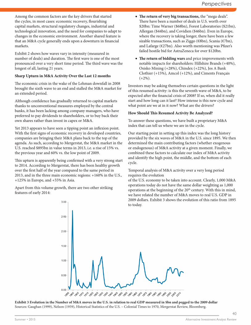
Perspectives
Alternative Investment Analyst ReviewSummer • 2015
40
Among the common factors are the key drivers that started the cycles, in most cases: economic recovery, flourishing capital markets, structural regulatory changes, industrial and technological innovation, and the need for companies to adapt to changes in the economic environment. Another shared feature is that an M&A cycle generally ends upon a downturn in financial markets.
Exhibit 2 shows how waves vary in intensity (measured in number of deals) and duration. The first wave is one of the most pronounced over a very short time period. The third wave was the longest of all, lasting 21 years.
Sharp Upturn in M&A Activity Over the Last 12 months
The economic crisis in the wake of the Lehman downfall in 2008 brought the sixth wave to an end and stalled the M&A market for an extended period.
Although confidence has gradually returned to capital markets thanks to unconventional measures employed by the central banks, it has been lacking among company managers, who have preferred to pay dividends to shareholders, or to buy back their own shares rather than invest in capex or M&A.
Yet 2013 appears to have seen a tipping point an inflexion point. With the first signs of economic recovery in developed countries, companies are bringing their M&A plans back to the top of the agenda. As such, according to Mergerstat, the M&A market in the U.S. reached $895bn in value terms in 2013, i.e. a rise of 15% vs. the previous year and 60% vs. the low point of 2009.
This upturn is apparently being confirmed with a very strong start to 2014. According to Mergerstat, there has been healthy growth over the first half of the year compared to the same period in 2013, and in the three main economic regions: +160% in the U.S., +125% in Europe, and +55% in Asia.
Apart from this volume growth, there are two other striking features of early 2014:
•The return of very big transactions, the “mega deals”. There have been a number of deals in U.S. worth over $20bn: Time Warner ($68bn), Forest Laboratories ($21bn), Allergan ($44bn), and Covidien ($46bn). Even in Europe, where the recovery is taking longer, there have been a few sizable transactions, such as Ziggo (€8bn), Scania (€7bn), and Lafarge (€27bn). Also worth mentioning was Pfizer’s failed hostile bid for AstraZeneca for over $120bn.
•The return of bidding wars and price improvements with notable impacts for shareholders: Hillshire Brands (+40%), Osisko Mining (+28%), Chindex (+22%), Jos A Bank Clothier (+15%), Amcol (+12%), and Ciments Français (+2%).
Investors may be asking themselves certain questions in the light of this resumed activity: is this the seventh wave of M&A, to be expected after the financial crisis of 2008? If so, when did it really start and how long can it last? How intense is this new cycle and what point are we at in it now? What are the drivers?
How Should This Resumed Activity Be Analyzed?
To answer these questions, we have built a proprietary M&A index that can tell us where we are in the cycle.
Our starting point in setting up this index was the long history provided by the six waves of M&A in the U.S. since 1895. We then determined the main contributing factors (whether exogenous or endogenous) of M&A activity at a given moment. Finally, we combined these factors to calculate our index of M&A activity and identify the high point, the middle, and the bottom of each cycle.
Temporal analysis of M&A activity over a very long period requires the evolution of the U.S. economy to be taken into account. Clearly, 1,000 M&A operations today do not have the same dollar weighting as 1,000 operations at the beginning of the 20th century. With this in mind, we have related the number of M&A moves to real U.S. GDP in 2009 dollars. Exhibit 3 shows the evolution of this ratio from 1895 to today.
Exhibit 3 Evolution in the Number of M&A moves in the U.S. in relation to real GDP measured in $bn and pegged to the 2009 dollar Sources: Gaughan (1999), Nelson (1959), Historical Statistics of the U.S. – Colonial Times to 1970, Mergerstat Review, Bloomberg.

41M&A Activity: Where Are We In the Cycle?
It emerges that the Great Merger Wave dwarfs the scale of the chart so much that it is difficult to draw conclusions about the current period. Moreover, we have seen that the latest cycle troughs of 2003 and 2009 almost match the mid-cycle levels for the second and third waves and are even above the top of the cycle for the fourth wave. We believe the explanation lies in the globalization of trade that took place in the early 1990sthat has had a notable impact on the M&A activity of the last two cycles, making the historical comparisons fairly irrelevant over a very long period. We have concentrated on the recent period of 1990 to the present day to identify the drivers behind M&A activity.
In studying M&A waves, we have seen that cycles often coincide with rising capital markets and an upturn in economic activity. Therefore, we tested the correlation of M&A activity with a series of factors related to equity and bond markets. We also studied the influence of parameters that we monitor as part of our merger
arbitrage strategy. We ultimately took four factors into account.
The first factor is the total capitalization of the U.S. market. For each quarter over the period in question, we set the total value of the operations announced over 12 rolling months against the total market capitalization of the U.S. market. Exhibit 4 shows that this ratio sits in a range of 2% to 4% for the bottom of the cycle and a range of 9% to 12% for cycle peaks.
The second factor is the FED Senior Loan Officer Surveys. On the basis of surveys among the main banking institutions, this indicator measures borrowing conditions for American companies and consumers. A high level reflects difficult borrowing conditions and a low level reflects easy conditions.
Exhibit 5 clearly shows that periods of decline in M&A correspond to times when borrowing becomes harder, as in 2000-2004 and 2008-2011.
Exhibit 5 Correlation between the FED Senior Loan Survey and the annual variation in M&A activity Sources: Mergerstat Review and Bloomberg
Exhibit 4 M&A Activity measured as a % of the total U.S. market capitalization Sources: Mergerstat Review, Wilshire Associates
0
200
400
600
800
1,000
1,200
1,400
1,600
0%
2%
4%
6%
8%
10%
12%
14%
$bn
Activité M&A en valeur mesurée sur 12 mois glissants (droite)
Activité M&A en % de la capitalisation boursière (gauche)M&A activity by value over 12 rolling months (rhs)
M&A activity as a % of stock market capitalisation (lhs)
-60%
-40%
-20%
0%
20%
40%
60%
80%
100%
120%
-80
-60
-40
-20
0
20
40
60
80
100
Variation annuelle de l'activité M&A (droite)FED Senior Loan Survey - 12 mois glissants (gauche)
Annual variation in M&A activity (rhs)
FED Senior Loan Survey – 12rolling months (lhs)
Exhibit 6 Correlation between the rate of expected improved bids and M&A activity Sources: Mergerstat Review and MAGMA
0
200
400
600
800
1,000
1,200
1,400
1,600
0%
10%
20%
30%
40%
50%
60%
70%
$bn
M&A activity by value measured over 12 rolling months (rhs)
% of M&A operations trading above the terms of the bid (lhs)
Exhibit 7 Correlation between the failure rate and annual variations in M&A activity Sources: Mergerstat Review and OFI AM
-60%
-40%
-20%
0%
20%
40%
60%
80%
100%
120%
0%
5%
10%
15%
20%
25%
1998 1999 2000 2001 2002 2003 2004 2005 2006 2007 2008 2009 2010 2011 2012 2013
Annual variation in M&A activity (rhs)
Failure rate of announced M&A operations (lhs)

Perspectives
Alternative Investment Analyst ReviewSummer • 2015
42
-2.0
-1.5
-1.0
-0.5
0.0
0.5
1.0
1.5
2.0
Stan
dard
dev
iatio
n vs
. his
toric
al a
vera
ge
Mid-cycle
Topo f cycle
Bottom of cycle
The third factor is an indicator that measures the number of improved bids expected by the market for M&A operations on listed companies. In certain cases when an M&A operation is announced on the markets, the share price of the target may be higher than the terms proposed by the prospective buyer. This means that investors are expecting an increase in the bid by the buyer or a counterbid by a third party. We have found this indicator to be a good measure of market players’ sentiment with respect to M&A activity. Exhibit 6 shows the movement of this indicator since 1998, as calculated from our proprietary MAGMA database.
We can clearly see that the high points and low points of this indicator coincide with the variations in the M&A activity cycle.
The fourth factor, also drawn from our MAGMA database, concerns M&A moves on listed companies. This is the failure rate of operations calculated over 12 rolling months, i.e. the number of terminated operations set against the number of completed operations. Several factors can lead to the failure of an operation: opposition of the target’s shareholders or antitrust authorities, financing problems, deterioration in market conditions, opposition of the buyer’s shareholders, etc. The average failure rate comes to about 7%. A significant increase in this rate above this average reflects a general rise in risk aversion within the M&A environment. Exhibit 7 shows the variations of this indicator over the period considered.
Once again, periods when M&A declines correspond to times when the failure rate is high.
To combine these four factors, we have standardized each of them by expressing a standard deviation from the historical average. We have then built our index by attributing a different weighting to each factor so that the index is as closely pegged to variations in M&A activity as possible.
Exhibit 8 shows the correlation between our proprietary index and activity and we can identify three zones:
1. The middle of the cycle: between -0.5 and 0.5 standard deviations from the average,
2. The top of the cycle: 1 standard deviation above the average,
3. The bottom of the cycle: 1 standard deviation below the average.
As Exhibit 9 shows, the index is currently around the upper part of the middle of the cycle. Over the last 12 months, we have seen a rebound in the index that logically follows a notable increase in the volume of M&A activity described earlier.
Detailed analysis of the four factors that make up the index shows that:
• Over Q2 2014, M&A volumes increased substantially faster than stock market indices, which resulted in a sharp rise in the first factor.
• Lending conditions are still very favorable to companies.
• The failure rate is still stable at around the historical average.
• Only the rate of improved bid expectations, which stands at around 40%, may reflect excessive optimism by operators. But the high number of improved bids observed shows that this enthusiasm among investors is not currently ill founded.
On the basis of this index, we can therefore consider that another M&A cycle has indeed started after the low point observed in 2009. From 2010 to 2012, M&A activity was modest and above all very chaotic, which is characteristic of a waiting period between two cycles. But since 2013, the upward trend appears to be well underway. With a very strong first quarter, 2014 looks like a good mid-cycle year.
Since it began in 2013, how long can this wave last?
It is particularly difficult to answer this question when, as we have seen, the previous waves lasted for very varied lengths of time: 7 years for the shortest and 21 years for the longest.
0
200
400
600
800
1,000
1,200
1,400
1,600
-2.0
-1.5
-1.0
-0.5
0.0
0.5
1.0
1.5
2.0
1992
1993
1994
1995
1996
1997
1998
1999
2000
2001
2002
2003
2004
2005
2006
2007
2008
2009
2010
2011
2012
2013
$bn
Stan
dard
dev
iatio
n vs
. his
toric
al a
vera
ge
M&A activity by value measured over 12 rolling months (rhs)
M&A index (lhs)
Exhibit 9 Top, Bottom and Middle of the M&A cycle index measured by standard deviation vs. the averageSources: OFI AM
Exhibit 8 Correlation between our proprietary M&A index and M&A activity Sources: Mergerstat Review and OFI AM
Top of cycle

43M&A Activity: Where Are We In the Cycle?
Even though we have not yet seen any signs of M&A activity overheating, there are still a number of events that could cause this latest cycle to finish prematurely:
• A rapid rise in interest rates in the U.S., which would make it harder to finance certain M&A operations. There would likely be a concomitant significant decline in equity markets, which would result in a loss of confidence among company managers who might postpone their M&A plans.
• A marked slowdown in U.S. growth following an exogenous shock hampering global trade, such as exacerbation of the crisis in the Ukraine, or renewed tensions in the Middle East.
All told, we think that this resumption in M&A activity marks the beginning of the seventh wave; we shall now try and identify its drivers.
Drivers behind this latest wave
We have seen that there is a common denominator for all M&A waves: economic recovery and its corollary, the flourishing of capital markets. But each wave also has its idiosyncrasies. We shall identify the specific drivers of the current wave in the light of the general macroeconomic context and the latest operations announced.
We think that one of the particularities is firstly in the notable time lag between the recovery of markets and the resumption of M&A activity in the U.S.; almost three years passed between the return of growth in Q3 2009 anticipated by the markets some months earlier and the resumption of M&A in 2012.
This particular situation was the result of non-conventional measures taken by central banks to support markets and the economy after the systemic crisis of 2009. Successive QE and near-zero interest rates saw mountains of liquidity pour into equity and bond markets, which then bounced back. Since 2009, the S&P 500 has posted an annual return of 22% and the IBOXIG of 9%.
But although confidence returned to the financial sphere fairly early in the cycle, with asset price inflation as a consequence, in the real economy it was lacking among company managers until very recently. Against an economic backdrop that they found uncertain at the time, companies preferred to adopt cautious strategies to grow their earnings per share: cost savings, investment constraints (on both capex and M&A), and share buybacks.
But these measures have now reached their limits: companies’ operating margins are at historical highs, organic growth has slowed due to low past investment, and for three years now share buybacks have been close to their highs of 2006-2007.
To contend with the forthcoming slowdown in profit growth, companies have moved into a phase where corporate finance transactions are set to become predominant in their industrial strategies. Moves recently announced by major groups clearly show the drivers that will be at work in this new phase:
• Reorganization around growth regions. For example, the Lafarge/Holcim merger will lead to the group repositioning towards emerging markets at the expense of mature countries.
• Transformation of business portfolios, like Novartis, which is moving away from vaccines and animal health and buying GSK’s oncology assets.
• Tax optimization. In the U.S., there is a tax inversion system at work that enables companies to drastically lower their tax. U.S. companies that buy a company abroad are able to relocate their HQ to the target’s country to pay less tax. With the high margins and profits generated by numerous subsidiaries around the world, this tax mechanism is of particular interest to pharmaceutical companies. The following deals in particular spring to mind: Warner Chilcott/Actavis ($7.8bn), Shire/AbbVie ($54.7bn), Valeant/Allergan ($54.2bn), and Covidien/Medtronics ($46.2bn).
• The use by American companies of cash located abroad. Taxation in the U.S. is rather special insofar as the financial flows of multinationals are taxed twice. Subsidiaries’ profits are taxed once in the country where they are generated and a second time when the parent company repatriates them in the form of dividends. All told, the U.S. has a marginal tax rate of 35%, one of the highest among industrialized countries. Consequently, U.S. companies prefer not to repatriate cash generated by their foreign subsidiaries. An acquisition can therefore be a good way to use this treasure trove. For example, with a cash pile of $90bn abroad, GE was in a position to bid $17bn for Alstom’s Energy division.
• Cross-border operations, particularly from the U.S. towards Europe, sweetened by the valuation difference between the two regions. Examples include the bid by Pfizer for British company Astrazeneca for $120bn, Liberty Media’s bid for the Dutch group Ziggo for $11bn, and the takeover of Telekom Austria by America Movil for $7bn.
It is important to emphasize that the tax inversion driver has been a significant contributor to the resumption of M&A since the end of 2013. We have identified 11 deals for a total of about $340bn, i.e. about 25% of the total over the period. However, the window of opportunity for tax inversion deals is probably closing.
These deals are seen as a form of tax evasion by American public opinion and caused quite a stir in the media in summer 2014. With the approach of mid-term elections, the issue has taken on a political dimension. Democrats have even proposed anti-inversion legislation to Congress, but this has run into opposition from the Republicans who would prefer to see a radical overhaul of the U.S. tax system. Meanwhile, the U.S. Treasury has grown impatient with the legal route and announced that it wants to make administrative changes to the tax code to make tax inversion moves much less appealing. In any case, there are a limited number of multinationals in the pharmaceutical sector in a position to fully benefit from tax inversion. The same goes for potential targets.
Although in the medium-term, the tax inversion driver is likely to carry less influence, the other drivers behind resumption of the M&A cycle should remain intact for the coming quarters: corporate confidence indices are at high levels, financing costs are low and there is the use of offshore cash for U.S. companies.

Perspectives
Alternative Investment Analyst ReviewSummer • 2015
44
Conclusion
We think that the resumption in M&A activity has now been in evidence for several quarters is the beginning of a new cycle, the seventh wave of M&A in the long economic history of the United States. Current M&A activity shows renewed confidence among managers who are now ready to embark on developmental external growth projects for the future of their companies. The index that we have built shows that we are currently in the middle of this new cycle.
DISCLAIMER
In the European Union, this document is only for the attention of “professional clients” (professional investors) as defined in Directive 2014/65/EC dated 15 May 2014 on markets in financial instruments (“MIFID 2”), to investment services providers and any other professional of the financial industry, and as the case may be in each local regulation and, as far as the offering in Switzerland is concerned, “Qualified Investors” within the meaning of the provisions of the Swiss Collective Investment Schemes Act (CISA), the Swiss Collective Investment Schemes Ordinance of 22 November 2006 (CISO) and the FINMA’s Circular 08/8 on Public Advertising under the Collective Investment Schemes legislation of 20 November 2008. In no event may this material be distributed in the European Union to “non-professional clients” (non-professional investors) as defined in the MIFID 2 or in each local regulation, or in Switzerland to investors who do not comply with the definition of “qualified investors” as defined in the applicable legislation and regulation.
This document is not intended for citizens or residents of the United States of America or to any “U.S. Person” as this term is defined in Securities and Exchange Commission Regulation S under the U.S. Securities Act of 1933.
This document is purely informative and has no contractual value, it neither constitutes an offer to buy nor a solicitation to sell, and shall not be considered as an investment advice.
OFI Asset Management accepts no liability whatsoever, whether direct or indirect, that may arise from the use of information contained in this material. OFI Asset Management can in no way be held responsible for any decision or investment made on the basis of information contained in this material. The information contained in this document is disclosed to you on a confidential basis and shall not be copied, reproduced, modified, translated or distributed without the prior written approval of OFI Asset Management, to any third person or entity in any country or jurisdiction which would subject OFI Asset Management or any of its funds to any registration requirements within these jurisdictions or where it might be considered as unlawful.
The information contained in this document is deemed accurate as at the date of publication set out on the first page of this document and may be changed without notice.
This article was initially written in September 2014.
Authors’ Bios
Fabienne Cretin Head of M&A Arbitrage, OFI Asset Management
Fabienne joined OFI AM in 2009 and is the head of the equity-related strategies of the group. Fabienne is also a Portfolio Manager of OFI Risk arbitrages and OFI Risk Arb Absolu funds. Prior to joining OFI AM, Fabienne was responsible for investing in Risk Arbitrage
and Special Situation funds within ADI Alternative Investments, where she worked for eight years. Previously Fabienne worked at Deloitte & Touche from 1997 to 2001 in the Mergers and Acquisitions division. Fabienne holds an MSc in Finance from ESSEC.
Stéphane Dieudonné Portfolio Manager, OFI Asset Management
Stephane joined OFI AM in 2009 as a Portfolio Manager of OFI Risk Arbitrages and OFI Risk Arb Absolu funds. Prior to joining OFI AM, Stephane worked for ADI Alternative Investments, where he was a Portfolio Manager within the Risk Arbitrage
and Special Situation funds team. From 2001 to 2004, Stephane worked for Kepler as an equity sell-side analyst covering various sectors. Prior to that, Stephane worked at Deloitte & Touche in the Mergers and Acquisitions division. Stephane graduated from HEC (Paris) and Supélec (Paris).
Slimane Bouacha Portfolio Manager, OFI Asset ManagementSlimane joined OFI AM in 2009 as a Portfolio Manager of OFI Risk Arbitrages and OFI Risk Arb Absolu funds. Prior to joining OFI AM, Slimane worked for ADI Alternative Investments, where he was a Portfolio Manager within the Risk Arbitrage and
Special Situation funds team. From 2002 to 2004, he held various positions within the financial industry: he was a sales assistant for the interest rate structured products division of Crédit Lyonnais and began his career as a Portfolio Manager assistant focusing in the Risk Arbitrage strategy. Slimane holds an MSc in Finance from University of Paris I.

Nowcasting: A Risk Management ToolAlexander Ineichen, CAIA Founder Ineichen Research & Management AG
Nowcasting
45Nowcasting: A Risk Management Tool
Nowcasting is to forecasting what astronomy is to astrology. At the beginning of 2014, 72 out of 72 economists “predicted” that U.S. interest rates would rise throughout the year. They fell. One ought to know what one doesn’t know. It’s always experts—often well-educated professionals who do not suffer from a lack of self-confidence—who create the forecasts; quite often keeping a straight face. Expert failure extends far beyond the investment scene. The problems often reside in man’s information processing capabilities. The expert is a serial or sequential processor of data who can only handle information reliably in a linear manner. Not only can experts analyze information incorrectly, they can also find relationships that are not there, a phenomenon called “illusionary correlation”. We suggest that investors replace forecasting with nowcasting.
What is nowcasting?
Nowcasting is a reasonably new word; at least in economic finance. It is either the opposite
of forecasting or simply a pun on the word ‘forecasting’. The term nowcasting is also a contraction of ‘now’ and ‘forecasting’. The term is used in both economics and meteorology. A forecaster tries to predict the future. Empirically, this has proven as quite a challenge in many endeavors related to human action. As Mark Twain succinctly put it: “Prediction is very difficult, especially if it’s about the future.”
We define nowcasting as follows:
Nowcasting is the economic discipline of determining a trend or a trend reversal objectively in real time. Nowcasting is fact-based, focuses on the known and knowable, and therefore avoids forecasting. Nowcasting is the basis of a robust decision-making process.1
A ‘nowcaster’ does not try to predict the future, but focuses what is known today, i.e., known now in real time. Forecasts are an integral part of orthodox asset allocation and are essentially guesswork. In other words, guessing is an

Nowcasting
Alternative Investment Analyst ReviewSummer • 2015
46
integral part of how assets are allocated and risk is taken and subsequently managed. However, some investors, for example trend-followers, seem to do very well without a forecast entering into their investment approach. Trend followers look at prices, not forecasts. A price is a fact, whereas a forecast is not; it is someone’s opinion that might or might not have merit. A forecast is biased by definition because it is an opinion. An investment process focussing on facts seems more logical than an investment process that focuses on opinions. A fact is a fact whereas an opinion is rather fluffy by comparison, and its merit often only assessable with the benefit of hindsight. Economist John Kenneth Galbraith put it most eloquently: “One of the greatest pieces of economic wisdom is to know what you do not know.”
A trend is a fact and is determinable. Momentum is one approach by which a trend can be determined. A trend is either positive or negative; essentially up or down. This makes investment life a lot simpler. Currently the economic trend in the U.S. is positive and the economic trend in Latin America isn’t. At one level, it’s that simple. The odds favour the former and not the latter.
This article examines three types of momentum: price, economic (top-down), and earnings (bottom-up) momentum. In the following sections some aspects related to these three approaches are discussed, starting with price momentum. The key take-away is the applicability for a pragmatic approach to risk management.
Price Momentum
The basic premise of momentum is that trends exist, i.e., there are cycles as opposed to complete randomness, and that trends are
determinable in real time, but the duration of the trend is nearly impossible to predict. Price momentum is the most common form of momentum, is well documented, and has stood the test of time. For late U.S. investor Martin Zweig (1942-2013), not going against the trend was a cardinal rule: “To me, the ‘tape’ is the final arbiter of any investment decision. I have a cardinal rule: Never fight the tape!” Going against the trend is akin to fighting an uphill battle; the odds are against you.
Exhibit 1 shows a screen shot from IR&M’s Momentum Monitor from 10 August 2014. The monitor shows positive and negative price momentum. (Positive momentum is here defined as the 10-week moving average exceeding the 40-week moving average and the momentum in the exhibit is measured in the number of weeks since the signal occurred. For example: The positive momentum in the MSCI World Index (first line) was in its 104th week in the 32nd week of 2014, resulting in a return of 31% since the signal occurred.)
Another example is China and Greece. China ended a 30-week bear market and entered a long-term bull market in week 32, as highlighted in Exhibit 1. The Greek stock market entered a long-term bear market around the same time. At the end of June 2015, these trends were still in place. From the time of the signal to the end June 2015, the Shanghai Composite gained 91% and the Athens SE General lost 24%.
A trend such as these could always end tomorrow, in which case a response by the investor is required. However, these trends could last a lot longer too. The main point is that no forecasting is required for the odds of the investor to be stacked in his favour.
Exhibit 1 Screen Shot of IR&M’s Momentum Monitor from 10 August 2014Source: IR&M

47Nowcasting: A Risk Management Tool
Although we all should have bought China A-shares and sold Greek stocks short in early August 2014, the main purpose of analyzing momentum is as a tool that adds systems and, ideally, an element of discipline to the investment decision-making process. Exhibit 1 from 10th August 2014 informed us that going forward we shouldn’t be long Greece and shouldn’t be short China. The risk management perspective is what not to do. The momentum analysis can add perspective from this angle.
Unfortunately, the analysis of price momentum does not tell us how long a trend lasts. One reason why knowledge of the trend is still valuable is because trying to forecast the reversal is such a foolish endeavour. Mean reversion is a powerful concept in finance. However, the nowcasting approach suggests measuring the reversion in real time, rather than hoping for it, or trying to forecast it. Here’s what we know when it comes to a trend, for example, the current bull market of the U.S. stock market: We know it’s a bull market. We know—and this is important—that we don’t know when it ends. Exhibit 2 shows the frequency distribution of U.S. bull markets of the S&P 500 price index since 1930. (We also know it’s an exceptional, liquidity-induced bull market.)
There were 50 bull markets as per our definition. The median duration of a long-term bull market is 54 weeks, i.e., roughly one year. 25 were 54 weeks or shorter and 25 bull markets were 55 weeks or longer than that. The current bull market was its 179th week as per Friday 26th June. How many times has the reader heard someone say the bull market is about to end during these 179 weeks? At the end of the bull market someone will eventually get it right by pure coincidence.
The current bull market could last a lot longer. Who knows? There is no limit to the time axis in Exhibit 2. The practical relevance is that one ought to be less risk averse in a bull market. In a bear market, bad news can have a large impact on price. This is different in a bull market. In a bull market, bad news might cause
small corrections that are used by the bull crowd to add stock in a generally rising market at lower prices. In a bear market this is much less likely to occur. After a long and/or violent bear market, at one stage unknowable without the benefit of hindsight, “bottom fishing” normally kicks in. However, we do not know when. When focusing on nowcasting rather than forecasting, i.e., astronomy rather than astrology; we do not need to know. We will be able to determine when the bottom fishers have become a force to be reckoned with, i.e., we can measure the price reversal, as with the Chinese stock market in week 32 of last year.
Economic Momentum
The best way to think about economic momentum is with a sailing analogy in combination with Minsky’s instability idea.2 Every sailor knows that a storm requires a different trim than calmer weather. IR&M’s gauge for economic momentum (the thin red line in Exhibit 3) is designed to indicate whether the economic environment is calm or a storm is brewing. The key is not to predict the next storm, but to respond when circumstances start changing. Rough weather at sea doesn’t change from one minute to the next. The same is true for a change of the economic winds; normally. There is time to trim the sails. In finance this means being more conservative or hedged when things start to change for the worse, i.e., the red line in the chart starts to fall. The storm’s zenith or magnitude and potential damage cannot be predicted in a continuous and robust fashion. However, changing circumstances can be measured and assessed at all times, making decision making more robust and therefore, in our view, more intelligent. The practical relevance to Minsky’s instability hypothesis is that, both at sea and in economics, the current calm is nothing else than the build-up of the next storm.
At the time of writing economic momentum in Germany was positive, an export-driven economy benefiting from a currency that was too weak. The practical implication is that the “economic wind” is blowing from behind.
Exhibit 2 Duration of positive long-term trends* in weeks since 1930 (S&P 500) Source: IR&M, Bloomberg * Long-term trend as defined in IR&M’s momentum monitor publication.

Nowcasting
Alternative Investment Analyst ReviewSummer • 2015
48
There always will be a next recession, in Germany and elsewhere. However, when economic momentum is positive, the likelihood of a recession within, say, a year is lower than if economic momentum were negative.
One aspect of economic modelling and an economic momentum approach is that it fails with, or doesn’t capture (or is slow to capture), political intervention. Monetary policy has “gained” as a market force under Alan Greenspan and has become more important ever since. Various central banks are battling a currency war; a race to the bottom, as some pundits put it. A central bank is not independent but is a part of the administration; it’s a political authority. (Central banks are independent in a sense that, if, for example, they run out of paper-clips, they can restock without involving the legislature officially.)
Below earnings momentum is discussed. Earnings momentum is essentially the bottom-up counterpart of the top-down economic momentum idea just discussed.
Earnings Momentum
The third part of the nowcasting toolkit is earnings momentum and is based on consensus earnings estimates from sell-side analysts. The preferred measure is the estimates for the next twelve months on a rolling basis, always hoping that the data provider gets the aggregation right. When looking at estimates it is important to distinguish between fact and opinion, i.e., nowcasting and forecasting. Earnings estimates falling from, say, 100 to 99 is a fact, but the “99” itself is an estimate and therefore subject to error. By comparison, 99 being lower than 100 is not subject to error.
Earnings momentum in the U.S. and Japan was mostly positive since the end of 2012. The subsequent USD returns of these equity markets to the end of June 2015 were 50% and 35% respectively. Earnings momentum in the Eurozone was flat and the USD return in this time period was 21%. Earnings momentum in the UK was the worst and was mostly negative and the USD
Exhibit 3 IR&M Germany (economic) model with DAX Index (as of 26th June 2015)Source: IR&M, Bloomberg
Exhibit 4 Twelve-month forward consensus earnings estimates indexed to 100 as of January 1, 2006 to June 30, 2015)Source: IR&M, Bloomberg
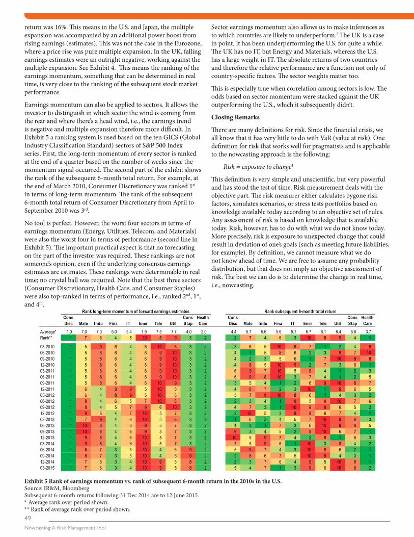
49Nowcasting: A Risk Management Tool
return was 16%. This means in the U.S. and Japan, the multiple expansion was accompanied by an additional power boost from rising earnings (estimates). This was not the case in the Eurozone, where a price rise was pure multiple expansion. In the UK, falling earnings estimates were an outright negative, working against the multiple expansion. See Exhibit 4. This means the ranking of the earnings momentum, something that can be determined in real time, is very close to the ranking of the subsequent stock market performance.
Earnings momentum can also be applied to sectors. It allows the investor to distinguish in which sector the wind is coming from the rear and where there’s a head wind, i.e., the earnings trend is negative and multiple expansion therefore more difficult. In Exhibit 5 a ranking system is used based on the ten GICS (Global Industry Classification Standard) sectors of S&P 500 Index series. First, the long-term momentum of every sector is ranked at the end of a quarter based on the number of weeks since the momentum signal occurred. The second part of the exhibit shows the rank of the subsequent 6-month total return. For example, at the end of March 2010, Consumer Discretionary was ranked 1st in terms of long-term momentum. The rank of the subsequent 6-month total return of Consumer Discretionary from April to September 2010 was 3rd.
No tool is perfect. However, the worst four sectors in terms of earnings momentum (Energy, Utilities, Telecom, and Materials) were also the worst four in terms of performance (second line in Exhibit 5). The important practical aspect is that no forecasting on the part of the investor was required. These rankings are not someone’s opinion, even if the underlying consensus earnings estimates are estimates. These rankings were determinable in real time; no crystal ball was required. Note that the best three sectors (Consumer Discretionary, Health Care, and Consumer Staples) were also top-ranked in terms of performance, i.e., ranked 2nd, 1st, and 4th.
Sector earnings momentum also allows us to make inferences as to which countries are likely to underperform.3 The UK is a case in point. It has been underperforming the U.S. for quite a while. The UK has no IT, but Energy and Materials, whereas the U.S. has a large weight in IT. The absolute returns of two countries and therefore the relative performance are a function not only of country-specific factors. The sector weights matter too.
This is especially true when correlation among sectors is low. The odds based on sector momentum were stacked against the UK outperforming the U.S., which it subsequently didn’t.
Closing Remarks
There are many definitions for risk. Since the financial crisis, we all know that it has very little to do with VaR (value at risk). One definition for risk that works well for pragmatists and is applicable to the nowcasting approach is the following:
Risk = exposure to change4
This definition is very simple and unscientific, but very powerful and has stood the test of time. Risk measurement deals with the objective part. The risk measurer either calculates bygone risk factors, simulates scenarios, or stress tests portfolios based on knowledge available today according to an objective set of rules. Any assessment of risk is based on knowledge that is available today. Risk, however, has to do with what we do not know today. More precisely, risk is exposure to unexpected change that could result in deviation of one’s goals (such as meeting future liabilities, for example). By definition, we cannot measure what we do not know ahead of time. We are free to assume any probability distribution, but that does not imply an objective assessment of risk. The best we can do is to determine the change in real time, i.e., nowcasting.
ConsDisc Mate Indu Fina IT Ener Tele Util
ConsStap
Health Care
ConsDisc Mate Indu Fina IT Ener Tele Util
ConsStap
Health Care
Average* 1.0 7.0 7.0 5.0 5.4 7.9 7.5 7.7 4.0 2.0 4.4 5.7 5.6 5.6 5.1 6.7 6.1 6.4 5.6 3.7Rank** 1 7 6 4 5 10 8 9 3 2 2 7 4 6 3 10 8 9 4 1
03-2010 1 5 9 6 4 6 10 8 3 2 3 6 5 10 8 7 1 2 4 906-2010 1 5 8 6 4 6 9 10 3 2 4 1 5 8 6 2 3 9 7 1009-2010 1 5 8 6 4 6 9 10 3 2 4 2 3 5 6 1 7 10 9 812-2010 1 5 8 6 4 6 9 10 3 2 4 8 5 10 9 2 7 3 6 103-2011 1 5 8 6 4 6 9 10 3 2 6 9 7 10 5 8 4 1 2 306-2011 1 5 8 6 4 6 9 10 3 2 6 9 8 10 3 7 4 1 2 509-2011 1 5 8 6 4 6 10 9 3 2 3 5 4 1 2 6 9 10 8 712-2011 1 6 4 8 9 5 10 6 3 2 4 8 7 2 3 10 1 9 6 503-2012 1 6 4 8 9 5 10 6 3 2 5 7 9 10 8 6 1 4 3 206-2012 1 8 4 6 5 7 10 8 3 2 2 3 4 1 9 5 8 10 7 609-2012 1 8 4 5 7 9 6 10 3 2 4 7 3 1 10 8 9 6 5 212-2012 1 9 6 4 7 10 5 7 3 2 2 10 5 3 9 8 6 7 4 103-2013 1 7 9 4 6 10 5 8 3 2 1 6 2 4 5 7 10 9 8 306-2013 1 10 8 4 6 9 5 7 3 2 4 2 1 7 3 6 10 9 8 509-2013 1 10 8 4 6 9 5 7 3 2 9 3 4 5 2 8 10 6 7 112-2013 1 9 8 4 6 10 5 7 3 2 10 5 9 7 4 2 8 1 6 303-2014 1 9 8 4 6 10 5 7 3 2 7 5 9 6 1 10 3 8 4 206-2014 1 8 7 3 5 10 4 6 9 2 5 9 7 4 3 10 8 6 2 109-2014 1 8 7 3 5 10 4 6 9 2 2 8 6 7 5 10 9 4 3 112-2014 1 7 6 3 4 10 9 5 8 2 2 3 7 6 4 9 5 10 8 103-2015 1 7 6 3 4 10 9 5 8 2 5 4 7 1 3 9 6 10 8 2
Rank long-term momentum of forward earnings estimates Rank subsequent 6-month total return
Exhibit 5 Rank of earnings momentum vs. rank of subsequent 6-month return in the 2010s in the U.S.Source: IR&M, Bloomberg Subsequent 6-month returns following 31 Dec 2014 are to 12 June 2015. * Average rank over period shown. ** Rank of average rank over period shown.

Nowcasting
Alternative Investment Analyst ReviewSummer • 2015
50
There is a saying that “a fool with a tool is still a fool.” This adage is highly applicable to the world of finance. Models and tools are imperfect and they misfire. However, an imperfect tool can be useful for the bottom line. A tool need not be perfect, nor does it need to stand alone. We believe a tool can be imperfect and be very useful by supplementing other analysis. The future is probabilistic; Grexit, Frexit, and Brexit might or might not occur, and —if they do occur—they might or might not have a material impact on ones’ portfolio. If a tool helps us to tweak our portfolio towards the probabilities being asymmetrically skewed in one’s favor; the tool adds value.
Examining price, economic, and earnings momentum are such tools. They are imperfect and should be used in conjunction with other analysis. However, these tools are good enough to attract the attention of both relative return and absolute return investors. The tools are battle-tested.
A further argument is simplicity. The world is not just probabilistic, it is complex too. We ought to simplify to understand what is going on. Most of the risk management literature is about risk measurement, not management. This was most likely a contributing factor of financial institutions becoming too comfortable with their risk measurement approaches prior to the 2008 financial crises. The mathematical complexity resulted in a communications gap between senior management and the risk measurement department, while the pseudo precision resulted in overconfidence in one’s own ability to control the situation. The momentum approach discussed herein is simple; it’s essentially red or green, and it’s unambiguous. There are no various shades of grey.
Risk is exposure to change. Nothing lasts forever. The situation will change eventually. Forecasting the change is a mug’s game. Applying nowcasting as a risk management tool allows the investor to spot the change in real time, will elevate the investor’s conviction in the change, and will therefore result in more disciplined and robust—and therefore more intelligent—decision making.
Endnotes
1. Ineichen, Alexander (2015) “Nowcasting and financial wizardry,” Risk Management Research, IR&M, January.
2. See Minsky, Hyman P. (1992) “The Financial Instability Hypothesis,” The Jerome Levy Economics Institute Working Paper No. 74 (May).
3. See Ineichen, Alexander (2015) “Sector momentum,” Risk Management Research, IR&M, June.
4. This definition is from the education materials of Chicago-based options trading boutique O’Connor in the late 1980s.
Author’s Bio
Alexander Ineichen, CAIA Founder Ineichen Research & Management AG
Alexander is the founder of Ineichen Research and Management AG, a research firm founded in October 2009 focusing on risk management, absolute returns, and thematic investing.
Alexander started his financial career in derivatives brokerage and origination of risk management products at Swiss Bank Corporation in 1988. From 1991 to 2005 he had various research functions within UBS Investment Bank in Zurich and London relating to equity derivatives, indices, capital flows, and alternative investments, since 2002 in the role of a Managing Director. From 2005 to 2008, he was a Senior Investment Officer with Alternative Investment Solutions, a fund of hedge funds within UBS Global Asset Management. In 2009, he was Head of Industry Research for the hedge fund platform at UBS Global Asset Management.
Alexander is the author of the two publications “In Search of Alpha: Investing in Hedge Funds” (October 2000) and “The Search for Alpha Continues: Do Fund of Hedge Funds Add Value?” (September 2001). These two documents were the most-often printed research publications in the documented history of UBS. He is also author of “Absolute Returns: The Risk and Opportunities of Hedge Fund Investing” (Wiley Finance, October 2002) and “Asymmetric Returns: The Future of Active Asset Management” (Wiley Finance, November 2006). Alexander has also written several research pieces pertaining to equity derivatives and hedge funds including AIMA’s Roadmap to Hedge Funds (2008 and 2012), which has been translated into Chinese and was the most-often downloaded document from their website at the time.
Alexander holds a Bachelor of Science in Business Administration with a major in general management from the University of Applied Sciences in Business Administration Zürich (HWZ) in Switzerland. Alexander also holds the Chartered Financial Analyst (CFA) and Chartered Alternative Investment Analyst (CAIA) designations and is a certified Financial Risk Manager (FRM). He is on the Board of Directors of the CAIA Association.

VC-PE IndexA Look at North American Private Equity as of Q4 2014Mike Nugent CEO/Co-Founder Bison
Mike Roth Research Manager Bison
VC-PE Index
51VC-PE Index
Mike Nugent CEO/Co-Founder Bison
Mike Roth Research Manager Bison
The final figures for 2014 are in and it was a good year for the venture capital industry. In addition to record fundraising and capital invested, returns in 2014 outpaced the rest of the industry. For the 2003 through 2012 vintage years, the median TVPI multiple for the North American VC industry grew faster than the buyout industry’s median TVPI multiple in 2014.
The VC industry’s distribution issue still remains though DPI ratios saw impressive growth in 2014. The fact remains that the buyout industry has been better at generating distributions. There is only one year (2010) from 1998 through 2011 where the median DPI ratio for the VC industry is higher than the buyout industry’s median DPI ratio.
For a more in depth look at the buyout and venture capital benchmarks, please visit www.bison.co.

Alternative Investment Analyst ReviewSummer • 2015
52
VC-PE Index
Exhibit 1 North America All Private Equity TVPI Benchmark
Exhibit 2 North America All Private Equity IRR Benchmark

53VC-PE Index
Exhibit 3 North America All Private Equity DPI Benchmark
Exhibit 4 North America All Private Equity Momentum Benchmark

Alternative Investment Analyst ReviewSummer • 2015
54
VC-PE Index
Author’s Bios
Mike Nugent CEO/Co-founder, Bison
Prior to founding Bison, Mike Nugent held senior roles at SVG Advisers, LP Capital Advisors and HarbourVest Partners, and has more than $3B in private market commitments to his credit. Mike started his career in the public markets with the
NASDAQ Stock Market, and also gained significant operating experience while running operations for a textiles manufacturer. He received his MBA from Boston College, and his BA from St. Bonaventure University. Mike lives on the North Shore of Massachusetts with his wife and two sons.
Mike Roth Research Manager, Bison
Mike Roth is the Research Manager at Bison and oversees the data collection and content production. Before Bison, Mike spent six years on the investment team at SVG Advisers. There, he conducted research and due diligence on buyout and venture capital
funds in the Americas. Mike received his BA in Economics from Boston College and is a CFA Level III candidate.

The Erosion of the Real Estate Home Bias: A U.S. Case Study in Risk DiversificationMax Arkey Vice President Product Management MSCI Real Estate
IPD Global Intel Report
55IPD Intel
As an asset class, real estate investing typically has a high degree of home bias, especially when compared to equities and fixed interest. However, this real estate home bias is starting to erode, with asset owners in most countries already investing internationally or actively exploring the options for building offshore exposures. Some of these asset owners are motivated purely by pricing, but many are also seeking diversification. This trend towards offshore investing is running in parallel with greater scrutiny from investment risk managers who want to integrate real estate risk analysis with other asset classes. The perceived diversification benefits of investing internationally may motivate risk managers to increase international exposure, but there are variations from country-to-country and investor-to-investor when it comes to the potential benefits. In this Global Intel Report MSCI explores the diversification benefit of international real estate for the US market.
Allocating From Home To Abroad
Real estate asset owners have historically been more inclined to invest directly in local assets. This preference for local assets typically stems from both greater familiarity with local markets and regulations as well as well as from a desire to simplify asset management practices. However, the traditional home-biased focus of real estate investing is starting to change with the globalization of real estate being driven by the largest Sovereign Wealth and Pension Funds, many of whom have explicit global mandates. There is also a broader trend, driven by recognition of the potential diversification benefits of international real estate exposure to investors. Most of these investors have started to understand the role of real estate in a multi-asset-class context, and this perspective tends to increase the demand for international real estate, further eroding home bias.

Alternative Investment Analyst ReviewSummer • 2015
56
IPD Intel
The appetite for international exposure across asset classes is demonstrated by surveys conducted by Towers Watson (for Equities and Bonds) and MSCI (for Real Estate). This work shows that the bias toward domestic investment is lowest for equities, but far higher for fixed income and for real estate. There is a logic for fixed income having a relatively strong home bias given its role in hedging domestic liabilities, but this appears somewhat less intuitive for domestic real estate as a hedging asset.
The trend of investors increasing exposure to international real estate raises questions about unforeseen risk implications, particularly in terms of how much overseas real estate is allocated in a portfolio, its geographic location risk, and the leverage that might be employed. The global financial crisis (GFC) taught investors that international diversification can be used to mitigate the risks of a strong downturn in an individual country. The GFC also revealed the extent to which inter-and intra-country correlations may increase in a crisis, emphasizing the need for
truly diversified global investment strategies to mitigate portfolio risk. The significant benefits of international diversification are illustrated in the chart that shows the return implications of different global exposures. Exhibit 2 compares the performance of the IPD Global Index with that of the IPD US Index (in blue) and the IPD Global Index series ex-US (in green). At a glance, it is possible to see the greater volatility of the US, particularly during the GFC. The chart also suggests that the IPD Global ex-US generates lower return but for far lower risk than a pure US exposure, leading to a higher return per unit of risk for ex-US exposure. This illustrates the benefits of international diversification, which are compounded when correlations benefits are taken into account.
One of the central benefits of international real estate is the significant differences that persist between countries. These differences are captured in Exhibit 3, which shows the historic return against the volatility of the main markets covered by the
Source: Towers Watson; MSCI Asset Owner Survey
30%36% 39%
44%
53%
62% 61% 64%70%
87%93%
98%
61%
79% 81%
90% 92% 95%
70%64% 61%
56%
47%
38% 40% 36%30%
13%7%
2%
39%
21% 19%
10% 8% 5%
0%
10%
20%
30%
40%
50%
60%
70%
80%
90%
100%
Cana
da
Switz
erla
nd UK
Japa
n
Aust
ralia US
Aust
ralia
Switz
erla
nd
Japa
n
UK US
Cana
da
Cana
da US
Aust
ralia
Switz
erla
nd UK
Japa
n
Domestic
ForeignEquities
(Domestic Avg: 43%)Bonds
(Domestic Avg: 79%)
Real Estate
(Domestic Avg: 83%)
Exhibit 1 Domestic and Foreign allocations across asset classes, 2013. Source: Towers Watson; MSCI Asset Owner Survey
Exhibit 2 Rationale for international real estate exposure: the US example, comparing US returns with the IPD Global Index and the IPD Global Index ex US Source: IPD

57IPD Intel
MSCI’s Barra risk model, with the size of the bubbles representing the size of the real estate markets. This chart shows that the US has tended to generate slightly below average performance with high volatility that contrasts, for instance, with France and Sweden, which have tended to generate higher returns for lower volatility. Although the chart excludes the issue of correlations between markets, it suggests that a US investor with overseas real estate exposure might benefit from risk reduction, while a German investor might benefit from return enhancement. The relatively high risk and low return Japan-based investor might, in contrast, benefit from both return enhancement and risk reduction from international exposure.
In the context of these different behaviors, it is possible to explore the trade-off between US and non-US real estate, and the implications of adding different levels of leverage to the international exposure. In this case, a loan-to-value ratio of 20
percent is assumed for the domestic real estate portfolio, taking the overall stand-alone risk up to 13.66 percent. The table in Exhibit 4 shows, in the green highlighted area, the impact of increasing the international real estate exposure by 20 percent increments with no leverage being added to the international exposure. This demonstrates the significant reductions in risk, from 13.66 percent for full domestic exposure to about 5 percent for full international exposure.
The table also shows the impact of increasing leverage for different levels of international exposure. In all cases, the addition of leverage increased risk but, for international exposure up to 40 percent, loan-to-value can be increased to 60 percent and result in a lower level of overall risk than a purely domestic portfolio. The table also shows that high levels of leverage, generally loan-to-value over 60 percent, had a significant impact on overall risk levels.
Portfolio Weights Global (ex USA) LTVUSA
LTV 20%Global
(ex USA) 0% 20% 40% 60% 80%
100 0 13.66 13.66 13.66 13.66 13.6680 20 11.56 11.73 12.02 12.61 14.5460 40 9.55 9.92 10.57 11.94 16.4240 60 7.68 8.32 9.42 11.73 19.0120 80 6.10 7.06 8.68 11.99 22.050 100 5.08 6.35 8.46 12.70 25.39
Note: Table assumes LTV = 0.2 for the USA Real Estate portfolio. Table varies LTV for the 30-country Global (ex USA) portfolio via short USD position. Calculations assume that currency risk is hedged for the Global (ex USA) portfolio vs USD base currency
Risk decreases through country diversification
Risk increases withaddition of leverage
Exhibit 3 Risk/Return characteristics of major global real estate markets. Source: IPD
Exhibit 4 Varying the nature of international real estate exposure for US investors. Source: IPD
Exhibit 5 Risk implications of exposure to different international real estate markets: The case of a US investor diversifying overseas. Source: IPD
0%
2%
4%
6%
8%
10%
12%
14%
2% 4% 6% 8% 10%1 2% 14%
Historic (10 year) Average Annual Returns (%)
US
Canada
Germany
JapanUK
France
AustraliaNZ
Note : Excludes South Africa( Return 18%, Risk 8%). Some Asian countries (China, Korea, Mal aysia, HK, Singapore, Ta iw an and Thailand) based on returns over 7 yea rs.
SwitzlerandSweden
NL
HK
China
Spain
Korea
Thailand
Italy
Denmark

Alternative Investment Analyst ReviewSummer • 2015
58
IPD Intel
These results demonstrated that market selection has significant risk implications. Given the relatively high volatility of the UK and its correlations with the US, there are smaller risk reduction benefits in building a purely UK international exposure.
The benefits were far greater for a Eurozone exposure, but the most significant benefits arose from exposure to the full range of markets in the IPD Global Index. Clearly, there was a range of scenarios that could be generated, but these examples illustrated the benefits of international exposure and how they could help drive portfolio construction as well as helping measure the risk of actual exposure.
Conclusion
The real estate home bias is starting to decline, with asset owners in many countries already investing internationally, or actively exploring the options for building such exposure. This trend is running in parallel with more risk managers seeking to integrate real estate risk analysis with other asset classes in their portfolios. The diversification benefits of investing internationally can significantly reduce the risk of real estate exposure. As always with real estate, the implications vary from country to country and investor to investor. A range of other factors also need to be considered, such as return objectives and the risks associated with implementation and market pricing. But these trends, complemented as they are by the increasing availability of real estate platforms through which investment can take place, are set to further erode the home bias that has, until recently, been a major characteristic of the real estate asset class.
Author’s Bio
Max Arkey Vice President Product Management MSCI Real Estate
Max Arkey works in product management at MSCI Real Estate where he heads up indexes and market information products. These analytics are mission critical to the
investment process for 19 of the top 20 largest global asset managers, all the way through to specialized domestic investors.
For further details contact: [email protected]\
About MSCI
For more than 40 years, MSCI’s research-based indexes and analytics have helped the world’s leading investors build and manage better portfolios. Clients rely on our offerings for deeper insights into the drivers of performance and risk in their portfolios, broad asset class coverage and innovative research. Our line of products and services includes indexes, analytical models, data, real estate benchmarks and ESG research. MSCI serves 98 of the top 100 largest money managers, according to the most recent P&I ranking.
©2015 MSCI Inc. All rights reserved

59Image Credits
Image CreditsImage Credits
Square Peg Round Hole 21 ©Yoel Ben-Avraham Image Source: https://www.flickr.com/photos/epublicist/3546059144
This image is being used under a Creative Commons Attribution NoDerivvatives 2.0 Generic license. (CC BY-ND 2.0)
Green Tree ©CAIA Association
Created by: Angel Cruz
Cycle ©CAIA Association
Created by: Angel Cruz
All other images are either in the public domain or have a Creative Commons non-Attribution license.

Alternative Investment Analyst ReviewSummer • 2015
60
Submission Guidelines
Article Submission: To submit your article for consideration to be published, please send the file to [email protected].
File Format: Word Documents are preferred, with any images embedded as objects into the document prior to submission.
Abstract: On the page following the title page, please provide a brief summary or abstract of the article.
Exhibits: Please put tables and graphs on separate individual pages at the end of the paper. Do not integrate them with the text; do not call them Table 1 and Figure 1. Please refer to any tabular or graphical materials as Exhibits, and number them using Arabic numerals, consecutively in order of appearance in the text. We reserve the right to return to an author for reformatting any paper accepted for publication that does not conform to this style.
Exhibit Presentation: Please organize and present tables consistently throughout a paper, because we will print them the way they are presented to us. Exhibits may be created in color or black and white. Please make sure that all categories in an exhibit can be distinguished from each other. Align numbers correctly by decimal points; use the same number of decimal points for the same sorts of numbers; center headings, columns, and numbers correctly; use the exact same language in successive appearances; identify any bold-faced or italicized entries in exhibits; and provide any source notes necessary. Please be consistent with fonts, capitalization, and abbreviations in graphs throughout the paper, and label all axes and lines in graphs clearly and consistently. Please supply Excel files for all of the exhibits.
Equations: Please display equations on separate lines. They should be aligned with the paragraph indents, but not followed by any puncuation. Number equations consecutively throughout the paper, using Arabic numerals at the right-hand margin. Clarify, in handwriting, any operation signs or Greek letters, or any notation that may be unclear. Leave space around operation signs like plus and minus everywhere. We reserve the right to return for resubmission any accepted article that prepares equations in any other way. Please provide mathematical equations in an editable format (e.g., Microsoft Word, using either Equation Editor or MathType).
Reference Citations: In the text, please refer to authors and works as: Smith (2000). Use parenthesis for the year, not brackets. The same is true for references within parentheses, such as: (see also Smith, 2000).
Endnotes: Please use endnotes, rather than footnotes. Endnotes should only contain material that is not essential to the understanding of an article. If it is essential, it belongs in the text. Bylines will be derived from biographical information, which must be indicated in a separate section; they will not appear as footnotes. Authors’ bio information appearing in the article will be limited to titles, current affiliations, and locations. Do not include full reference details in endnotes; these belong in a separate references list; see next page. We will delete non-essential endnotes in the interest of minimizing distraction and enhancing clarity. We also reserve the right to return to an author any article accepted for publication that includes endnotes with embedded reference detail and no separate references list in exchange for preparation of a paper with the appropriate endnotes and a separate references list.

61Submission Guidelines
Submission Guidelines
CAIA.org
References List: Please list only those articles cited, using a separate alphabetical references list at the end of the paper. We reserve the right to return any accepted article for preparation of a references list according to this style.
Copyright Agreement: CAIA Association’s copyright agreement form giving us non-exclusive rights to publish the material in all media must be signed prior to publication. Only one author’s signature is necessary.
Author Guidelines: The CAIA Association places strong emphasis on the literary quality of our article selections.
Please follow our guidelines in the interests of acceptability and uniformity, and to accelerate both the review and editorial process for publication. The review process normally takes 8-12 weeks. We will return to the author for revision any article, including an accepted article, that deviates in large part from these style instructions. Meanwhile, the editors reserve the right to make further changes for clarity and consistency.
All submitted manuscripts must be original work that has not been submitted for inclusion in another form such as a journal, magazine, website, or book chapter. Authors are restricted from submitting their manuscripts elsewhere until an editorial decision on their work has been made by the CAIA Association’s AIAR Editors.
Copyright: At least one author of each article must sign the CAIA Association’s copyright agreement form—giving us non-exclusive rights to publish the material in all media—prior to publication.
Upon acceptance of the article, no further changes are allowed, except with the permission of the editor. If the article has already been accepted by our production department, you must wait until you receive the formatted article PDF, at which time you can communicate via email with marked changes.
About the CAIA Association
Founded in 2002, the Chartered Alternative Investment Analyst (CAIA) Association® is the international leader in alternative investment education and provider of the CAIA designation, the alternative industry benchmark. The Association grants the CAIA charter to industry practitioners upon the successful completion of a rigorous two-level qualifying exam. Additionally, it furthers the Association’s educational mandate through the dissemination of research, webinars, and videos. CAIA supports three publications for members: AllAboutAlpha.com, The Journal of Alternative Investments, and the Alternative Investment Analyst Review. CAIA members connect globally via networking and educational events, as well as social media.

Chartered Alternative Investment Analyst Association®Q3 2015, Volume 4, Issue 2