Alternative beta - UBS Global topics · Minimum expected tail loss ... alternative beta ... measure...

1

Alternative betaRisk premia investing that is more targeted in nature than broad market beta.

Asset managementProfessional clients only

2

Contents

Introduction 3

Building smarter value equity strategies 6

Minimum expected tail loss equity portfolios 11

Tactical tilts and multi asset class risk premia 14

Your global investment challenges answered 18

Contact 19

Contributing authorsArt GreshAdam JokichAndreas RazenPatrick Zimmermann

© UBS 2016. The key symbol and UBS are among the registered and unregistered trademarks of UBS. All rights reserved.

3

Smart beta, factor beta, strategic beta ... it goes by many names; we prefer the term alternative beta. What it generally refers to is risk premia investing that is more targeted in nature than broad market beta. Its origins lie in early quantitative investment approaches that seek to add value using factor based models for identifying what are now familiar return drivers, e.g. value, momentum, size and quality to name a few. Although initial applications have primarily been focused on equity markets, the alternative beta concept can also be applied to other asset classes such as fixed income and commodities.

One could argue then that alternative beta has been a feature of some quantitatively managed investment strategies for quite some time. Where alternative beta differs from its active, quantitatively managed counterparts, is in its level of transparency. Put simply, this takes the form of simple rules-based methods for portfolio construction or, in an analogy to traditional passive investing, indexing by a means other than market capitalization. Indeed it is in part the relative simplicity and transparency of the alternative beta approach that has led to its adoption by an increasing number of investors.

However, as investors' interest in alternative beta strategies has grown, so have their questions. Investors often find it challenging to choose between a growing field of providers that purport to offer the same alternative beta exposures. Methodologies differ across providers. Are these differences meaningful in terms of capturing the beta exposure in question? Do process differences lead to economically different outcomes? Perhaps even more fundamental are questions regarding how alternative beta strategies can be used in practice. How should alternative beta strategies be combined or packaged and how might alternative beta vehicles be employed as instruments for factor beta based allocation?

What follows is our attempt to explore these questions and present them within the context of three examples. Each has been selected in response to specific client queries. We do not contend that what we present is an exhaustive treatment of the subject. Rather we hope it will be illustrative of our approach to the topic and UBS Asset Management's contribution to the discussion.

The first paper focuses on what is perhaps the most well-known and thoroughly studied factor, premium:value. Both practitioners and academics have devoted considerable effort to:

– In the case of the former, developing investment processes utilizing valuation techniques, and

– In the case of the latter, testing alternative rationales for the existence of the value premium.

Introduction

4

That said, it is the apparent persistence of the value premium across markets and asset classes that has resulted in its emergence as one of the largest asset categories in the alternative beta space. The research here examines the value premium in the equity market, specifically focusing on how the premium is measured and how the resulting indices are constructed.

Our research indicates that the methods typically employed by most index providers can be improved upon with relatively modest effort. In particular, we find that measuring value using customized metrics that reflect the specific industry / sector dynamics and structure leads to superior results compared to techniques typically employed by most alternative beta index providers where an almost identical list of metrics is used for each and every sector. The fundamental insight here can be simply stated by way of an example: Utility companies are very different to Technology companies so why would we use the same metrics or ratios to measure value in both of these sectors? A superior approach is to use our fundamental understanding of these sectors to develop sector specific metrics that better measure and capture the value premium.

Our second paper examines the factor risk premium that rivals, if not exceeds, value in terms of asset flows and client interest – low-risk. In particular, we focus on the variant of the low-risk premium termed 'Minimum Volatility'. Minimum Volatility investing has expanded dramatically in the years following the Financial Crisis and while the desire on the part of investors to mitigate losses is understandable given the searing experience of Autumn 2008, we question whether a Minimum Volatility strategy is the best means of securing this objective.

A Minimum Volatility approach defines risk, as the name implies, in terms of volatility. For a portfolio of stocks, this means that the portfolio's volatility is determined by the underlying volatilities and correlations of the stocks held in the portfolio. Unfortunately, volatility only adequately describes the risk an investor faces under fairly restrictive assumptions. In the real world of markets, the assumptions are nearly always violated:

– Correlation only captures linear relationships

– The co-movements of stocks are often non-linear, especially in times of crisis. Volatility is only an adequate descriptor when returns are normally distributed

– Empirical evidence demonstrates that returns are more extreme than what can be supported under the assumption of log normality, as the following papers will highlight.

Finally, the nature of the volatility statistic makes it at best a partial solution to the investor's problem of minimizing drawdown. Volatility is a symmetric measure. A process that minimizes volatility not only reduces downside potential but also reduces upside potential.

5

Art GreshManaging DirectorUBS Asset Management

In order to address investors' concern over loss mitigation, we propose constructing a portfolio around a risk measure that better captures the non- linearities and non-normality of the distribution of stock returns. The measure we use is Expected Tail Loss (ETL). ETL allows us to estimate the features of the distribution that cannot be adequately captured using volatility. The richer measure of risk that ETL affords allows us to better target portfolio drawdown risk. Additionally, ETL has the benefit of not explicitly compressing the exposure to the upside of the distribution. Our simulation results show the ETL approach achieving superior risk adjusted returns and lower drawdowns than those achieved using Minimum Volatility.

The third paper is an example of how an investor might use alternative beta strategies as building blocks in a multi-asset portfolio. Where our previous discussion has focused exclusively on equities, this piece of research introduces additional sources of alternative beta from fixed income, foreign exchange and commodities. The alternative beta elements form the core of the portfolio in much the same way as conventional market capitalization indexed passive strategies often form the components in a traditional asset allocation strategy. Construction of the core portfolio is governed by a modified risk parity approach where the marginal contribution of each factor's risk component is equalized subject to a risk budget constraint at the asset class level (e.g., 50% fixed income, 40% equity and 10% commodities).The paper then goes on to explore ways that the core portfolio can be improved by a series of enhancements. The most relevant of these enhancements in terms of alternative beta premia is the introduction of macroeconomic tilts. The tilts imposed are a function of the macroeconomic cycle and take the form of deviations from the core risk parity portfolio aligned with that cycle. As an example, while in the recessionary phase of the cycle the portfolio would tilt toward Minimum Volatility and equity yield factor premium.

The work presented here is just one of many potential alternative beta applications in the multi-asset context. For those interested in learning more, we encourage you to read the individual papers. We hope you find them useful in framing your own questions, and answers, on the appropriate use of alternative beta strategies in your portfolio or that of your clients.

6

Building smarter value equity strategies

Introduction and overviewValue investing is perhaps the most well-established of investment principles. Its core tenet implies that investors can earn superior returns by preferring cheap assets over expensive ones. It is the basis of modern security analysis in which analysts attempt to discern the value of a security by assessing that security's underlying fundamentals. For decades this has been the process which has guided traditional active management.

In recent years, investors have begun to explore systematic approaches to capture what has come to be termed 'the value premium'. In an effort to harvest the observable value premium in the market, nearly all large index vendors have devoted resources to the development and marketing of value indices. In general these indices are of two broad types. The first utilizes the concept of fundamental weighting which derives constituent weights from the underlying company fundamentals. The rationale behind fundamental weighting is that over the long term, weighting the universe by fundamental measures, rather than prices, will guard against market bubbles and crashes as deviations between fair price and fundamental value can be long-lived. These types of strategies employ a combination of sales, operating cash flow, uses of cash, and book value to determine the weight of the company in the index. By construction, fundamental indexing has historically exhibited a tilt towards value versus its capitalization weighted universe.

The second method directly incorporates price level valuation ratios for the security selection and index construction process. In practice, this approach is typically implemented by first computing a composite value score for each company using valuation metrics such as price to earnings and price to book value. The index constituents and their respective weights are then determined largely by a security's market capitalization and value score. A value tilt is a natural by-product of the relative value metrics employed in the security selection and index construction process. The primary objectives of these indices are to maintain a significant exposure to value, while also aligning closely with its capitalization weighted index. To achieve both objectives, constraints may be imposed when constructing the index, such as target holding counts and sector neutrality relative to its capitalization weighted index (i.e. zero active sector bets).

A feature common to both the fundamental and price-relative indexing approaches is each methodology's almost uniform application of the same fundamental ratios / value metrics across all sectors and industries. Aside from Financials, most indices are naively constructed using the same valuation metrics across all industries, and fail to recognize the heterogeneity in industry dynamics and return drivers across industries.

Introducing industry specific metricsGiven the above, a natural extension of current practice is the introduction of industry specific valuation metrics, ones that better reflect the idiosyncrasy of each industry structure. Consider Financials, a sector that contains industries with differing market cycle dynamics. For example, the revenue stream and capital requirements of Real Estate companies are significantly different to those of Insurance companies.

Going a bit deeper, let us examine the construction methodology of the value score used by MSCI in the construction of their MSCI Enhanced Value suite. These indices use an equally weighted average of the forward Price to Earnings (P/E), Enterprise Value (EV) to Cash Flow from Operations (CFO), and Price to Book Value (P/B) in the computation of the composite value score, with the exception of the Financials sector. Within the Financials sector, companies are measured based on forward Price to Earnings (P/E) and Price to Book (P/B). While all three components have been shown to exploit different aspects of a company's value, these signals should not be applied uniformly across the market. For example, the P/B ratio tends to work well when firms have large amounts of fixed assets on their balance sheet, however, the efficacy of this ratio will suffer when companies have large, intangible assets (e.g. brand names, patents).

These observations lead to the question: How well does the MSCI Enhanced Value methodology identify over or undervalued companies, using the three aforementioned factors uniformly across all sectors?

7

Figure 1MSCI Financials Valuation Signal Monthly returns for the top 25% of companies (most attractive) in the MSCI World Index based on their valuation score, versus the bottom 25% of companies (least attractive) in the MSCI World Index. The valuation scores are calculated using the same methodology used to constructed the MSCI World Enhanced Value Index, which is an equally weighted average of the forward Price to Earnings (P/E) and Price to Book Value (P/B) value.

20

40

60

80

100

120

140

160

Top 25% Wealth relative

2007 2008 2009 2010 2011 2012 2013 2014 2015 2016

Bottom 25%

Source: UBS Asset Management. For details of computation see footnote 1 on page 10. See disclosures for important information regarding simulated results.

Figure 1 presents the results of a simple back-test where we attempt to answer this question. Using the MSCI Enhanced Value methodology, and the MSCI World Index as our universe, we create two equally weighted portfolios based on their assigned value score, one of the top quartile (under-valued), and one of the bottom quartile (over-valued), and plot their respective returns over time. With approximately 1,600 companies in the MSCI World Index, selecting the top quartile provides adequate breadth within each sector, and is well aligned with the MSCI World Enhanced Value Index target of 400 companies. We also plot the wealth relative line (i.e., the difference in return between the top and bottom 25% of companies, based on their value score). Examining the results we see little difference in the performance of the top and bottom 25% of the distribution.

These results suggest an industry specific mapping may be merited. Our approach draws upon the knowledge of our global fundamental analysts. We use their understanding of the industry dynamics to identify the appropriate metrics for each industry in the Financials sector. The Financials sector is comprised of industries with significantly different business models and thus, each should be valued using valuation metrics that are specific to that industry. Like MSCI, we believe Price

to Book (P/B) and Forward Earnings Yield (E/P) have persistently proved to add value across the Financials sector and broader global equity markets. The two aforementioned factors provide a base for valuing Banks and Insurance companies. Specifically, Price to Book is a critical measure in assessing the value of a company within these industries. Given much of their value is derived from capital markets, they are required to mark-to-market their assets and liabilities on the balance sheet, which gives investors an accurate assessment of shareholders' equity at fair value.

However, within the Diversified Financials and Real Estate industry, Price to Book (P/B) proves to be of less importance. Unlike Banks and Insurers, the assets and liabilities for Real Estate companies are not liquid, and prices are not readily available in the capital markets; this requires investors to carefully scrutinize Price to Book ratios across companies as the book values may be distorted.

Further, much of the Real Estate industry, specifically REITs, are heavily regulated and forced to distribute a large portion of earnings to shareholders. As a result, the current dividend yield and sustainability of the dividend policy are critical in assessing the value of REITs. Monitoring the ongoing operating cash flow through its reported Funds from Operation (FFO) is a more accurate measure of a REIT's sustainable profitability than the standard Cash Flow from Operations (CFO). Specifically, the latter often includes many one-time items, such as gains / losses from the sale of property and reported changes in the equity positions of unconsolidated entities. The NAREIT definition of FFO strips out these non-recurring and / or non-cash line items, allowing investors to better ascertain the ongoing cash earnings from the real estate business. Additionally, given the capital intensive nature of the Real Estate industry, we believe EBITDA Yield gives a clearer reflection of the business operations when compared to Earnings Yield, as it is irrespective of the financing and depreciation / amortization decisions.

Lastly, as mentioned above, dividend policy is critically important in valuing companies in the Real Estate industry, but total yield, which includes net share buybacks, is more suitable for Banks and Insurance companies, given their preference and history of share buybacks.

8

With these customized industry specific valuation measures we repeat the analysis we presented above. The results of this exercise are presented in Figure 2. Inspecting the results we now see better separation between the top 25% of most attractive companies (under-valued) and the bottom 25% of least attractive companies (over-valued). Figure 3 presents further evidence of this improvement. Here we plot the histograms of the monthly return spreads (Top 25% - Bottom 25%) using both the methodology used in constructing the MSCI World Enhanced Value Index and UBS Asset Management approaches. It is clear that the UBS AM histogram has shifted rightward relative to that of the MSCI. This indicates that a greater return differential between the top and bottom quartile is captured using industry specific valuation metrics. A 99% confidence t-test for mean equality confirms the average UBS return spread is greater than the return spread using the MSCI Enhanced Value methodology.

Figure 2UBS Financial Valuation SignalMonthly time series of returns for the top and bottom 25% of the sorted Financials sector based on UBS scoring methodology customized for the Financials sector. Portfolios are indexed to 100 as of December 31 2007 and tracked through to April 30, 2016.

20

40

60

80

100

120

140

160


2007 2008 2009 2010 2011 2012 2013 2014 2015 2016

Bottom 25%

Source: UBS Asset Management. See disclosures for important information regarding simulated results.

Figure 3Return Spreads for Financial SignalsDistribution of monthly return spreads between the top and bottom 25% of the sorted sector. Returns are from December 31, 2007 – April 30, 2016

Number of months

0

10

20

30

40

50

-10 -8 -6 -4 -2 0 2 4 6 8 10

UBS MSCI Return spread between top and bottom portfolios in %

Source: UBS Asset Management

9

Next, we extend the industry specific approach across all MSCI GICS Sectors in the MSCI World Index to create a well-diversified portfolio of the top 25% (most attractive based on valuations) and bottom 25% (least attractive based on valuations) of companies in each sector, using both, the methodology employed by the MSCI Enhanced Value suite and the UBS AM approach. The sector specific and well-diversified portfolio results of this exercise are presented in Table 1. We see that for most sectors, and in the well-diversified portfolio, using industry specific valuation metrics improves the top minus bottom return spreads.

Figures 4 and 5 tell the same story for the well-diversified portfolio we observed in the Financials sector. It is evident that using valuation factors uniformly across all sectors, as employed by the MSCI Enhanced Value suite, does not do an adequate job in distinguishing the difference between over and undervalued companies across all sectors. In contrast, using industry specific valuation factors provides a clearer distinction between the top and bottom quartiles, thus better capturing the value premium. As shown in figure 5, the spread distribution between the most attractive and least attractive well-diversified portfolios are persistently greater using the UBS AM approach relative to the methodology employed by the MSCI Enhanced Value suite; the results are confirmed to be statistically significant using a t-test for mean equality. It is apparent that using industry specific valuation factors is the superior methodology across many of the MSCI GICS sectors, as shown in Table 1 on the following page.

Figure 5Well-diversified portfolioMonthly time series of well-diversified portfolios. Well-diversified portfolios are created by aggregating the top and bottom 25% of companies in each MSCI GICS sector based on valuation using the UBS AM and MSCI Enhanced Value Index methodology. Portfolios are indexed to 100 as of 31 Dec 2007and extend until April 30, 2016

MSCI Enhanced Value Index methodology UBS AM methodology

40

60

80

100

120

140

160

180


2007 2008 2009 2010 2011 2012 2013 2014 2015 2016

Bottom 25%

40

60

80

100

120

140

160

180


2007 2008 2009 2010 2011 2012 2013 2014 2015 2016

Bottom 25%


Figure 4Return Spreads for the well-diversified portfolios using MSCI World Enhanced Index methodology and UBS AM methodology Distribution of monthly return spreads between the most attractive (top 25% under-valued) and least attractive (bottom 25% over-valued) well-diversified portfolios. Returns are from December 31, 2007 – April 30, 2016.

Number of months

0

5

10

15

20

25

30

35

-6 -5 -4 -3 -2 -1 0 1 52 3 4 6

UBS MSCI Return spread between top and bottom portfolios in %


10

ConclusionThis study examines some potential limitations of off-the-shelf / one-size-fits-all products that seek to capture the value premium. Careful consideration should be placed on metrics used to measure value and the process of signal construction. It is imperative to realize that for strategies attempting to take advantage of the value premium, the input signals need to be defined in a manner that will segment the market effectively as no portfolio construction technique will compensate for inefficient underlying signals. The value premium still exists, but as the market evolves, smarter signal construction is necessary in order to capture it.

1 Simulation is based on a subset of equity constituents in the MSCI World index, in USD, gross of fees and transaction costs. Simulated portfolio was rebalanced monthly. The dividend criteria used for stock selection is net of non-reclaimable withholding tax dividend yields from a Luxembourg domicile‘s perspective, but returns are based on total returns. Simulation is hypothetical and does not represent a live track record or actual returns realized by any investor. Past performance, whether simulated or actual, is not a guarantee for future performance. See disclosures for additional information.

Table 1Return Spreads SummaryAnnualized returns comparing the methodology used by the MSCI World Enhanced Value Index and UBS AM. Returns are an equal weight of the top 25% (most attractive based on valuation) and bottom 25% (least attractive based on valuation) of companies in each sector. The well-diversified portfolio is an equally weighted sector portfolio. The returns are from December 31, 2007 to April 30, 2016.

AssetMSCI

Top 25%MSCI

Bottom 25%

MSCI Annualized Difference

UBSTop 25%

UBSBottom 25%

UBS Annualized Difference

Difference inAverage Spreads

(UBS-MSCI)

1

Consumer Discretionary 6.3 8.4 -1.3 5.2 7.5 -1.6 -0.3

Consumer Staples 8.2 6.8 1.3 11.6 6.2 4.9 3.6***

Energy -2.1 -5.8 3.6 -0.3 -6.5 6.3 2.7***

Financials -1.7 1.0 -1.1 0.2 -2.1 3.4 4.5***

Industrials 14.3 11.1 2.2 15.2 12.2 2.2 0.1***

Health Care 4.6 2.2 2.8 5.8 1.3 5.0 2.1

Information Technology 5.5 5.3 0.1 5.6 4.6 0.9 0.8

Materials -1.3 3.7 -3.7 1.5 -0.5 1.8 5.5***

Telecommunications 7.8 6.2 0.8 7.4 6.7 -0.3 -1.1

Utilities 2.9 1.1 1.4 3.5 -1.6 5.0 3.6***

Well-Diversified Portfolio 5.0 4.4 1.1 6.1 3.2 3.2 2.1***

1 Significance level based on P-value from T-Test with hypothesis of UBS mean spread > MSCI mean spread without assumption of equal variance * Significant at 10% level, ** Significant at 5% level, *** Significant at 1% level

2 Methodology shown in Figure 6 and Figure 7Past performance, whether simulated or actual, is not a reliable indicator of future results.Source: MSCI, UBS Asset Management, 31 Dec 2005 – 31 Dec 2014 (Returns in USD)See disclosures for important information regarding simulated results.

11

Minimum expected tail loss equity portfolios

IntroductionThe wealth eroding losses experienced in the Financial Crisis of 2008 have driven interest in low risk equity strategies. These include minimum volatility, inverse variance weighted, equal weighted, maximum diversification and equal risk contribution. The most popular, by far, has been minimum volatility portfolio construction. As the name suggests, minimum volatility strategies seek to reduce the volatility of expected returns thereby decreasing expected losses but also limiting upside exposure.

Minimum volatility investing has some support in academic literature: studies have shown it to be consistent with the behavioral notion of loss aversion bias, where investors strongly prefer loss avoidance to acquiring gains – see Tversky and Kahneman 19911. This note takes a closer look at minimum volatility investing and considers an alternative we find more appealing.

A closer look at Minimum VolatilityMinimum volatility portfolio construction has its origins in Modern Portfolio Theory (MPT) which holds that under fairly restrictive assumptions, investors' preferences can be described using two statistical variables: expected return (mean) and risk (variance). It's important to note that the minimum volatility portfolio is not simply a collection of stocks with the lowest individual volatilities; rather, it is the outcome of a mean- variance optimization that exploits the opportunities for cross stock diversification, where the required inputs are individual stock volatility and cross stock correlation estimates. However, the conditions where the mean-variance framework adequately captures the full dimensionality of risk facing the investor are rarely met in practice.

Let's investigate this proposition further by looking at the co-movement of stocks. In a mean-variance world this co-movement is sufficiently measured by cross stock correlation. Correlation is, of course, a linear measure of association. Observation, however, suggests the co-movement of stocks can be non-linear / unstable at times. Consider that the diversification effect is dependent on robust correlation estimates, which are typically estimated using historical data.

Then consider the case where most of the estimation window corresponds to a relatively calm state of the market. This leads to issues during market turmoil when correlations are known to increase drastically; just when diversification is urgently needed. Under this minimum volatility methodology, the correlation estimates do not accurately reflect the relationships between assets in this high risk environment and are ill-equipped to provide diversification during extreme conditions.

Further, the mean-variance framework upon which minimum volatility is based, assumes that stock returns are normally distributed. If this assumption were to hold then a plot of the histogram of stock returns would be bell shaped and symmetric with thin tails. But, in fact, this is not what we observe. As an illustrative example, Xiong (2010)2 points out that observations drawn for a normal distribution with the same standard deviation for the S&P 500 (measured from January 1926 – April 2009) predict a return of -15.5% to occur just over once in 83 years. In point of fact, the S&P 500 suffered a monthly loss of greater magnitude in at least 10 instances during the same measurement interval.

Finally, and perhaps most importantly, volatility has some properties that may make it a less desirable measure of risk from an investor's perspective. Recall, volatility is a statistic that describes how observations are dispersed around the average value. Its symmetrical nature means that values below and above the average both contribute equally. Minimizing the volatility of a portfolio limits negative portfolio returns as desired; however, minimizing volatility will also decrease positive returns. A preferable low risk strategy would lower the magnitude of losses but preserve the ability of the portfolio to recover quickly. After a 20% portfolio drawdown, a 25% gain is required to climb out of the trough as a result of the lower asset base. The portfolio constructed to minimize volatility limits downside exposure but it also restricts upside potential.

With the caveats cited above in mind, we now examine another approach, one which attempts to address the apparent pitfalls and limitations of minimum volatility portfolio constructions.

1 Tversky & Kahneman (1991) "Loss Aversion in Riskless Choice: A Reference-Dependent Model" The Quarterly Journal of Economics2 Xiong, J. (2010) "Nailing Downside Risk" Journal of Risk Management

12

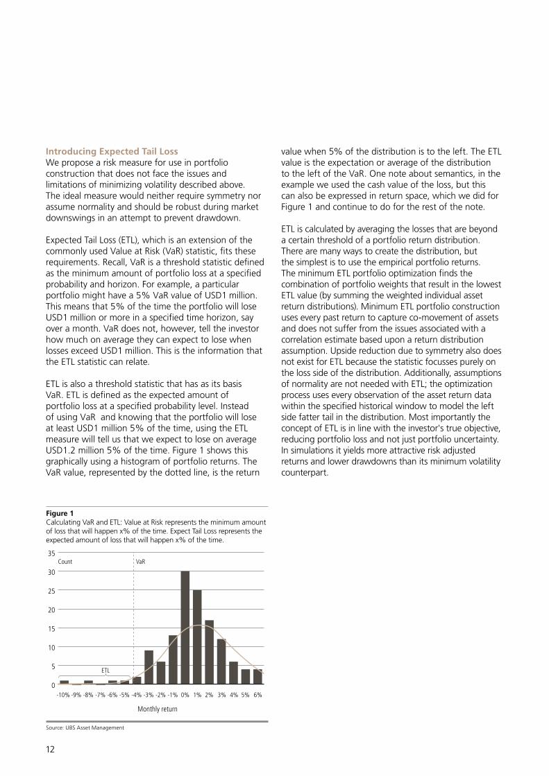
Introducing Expected Tail LossWe propose a risk measure for use in portfolio construction that does not face the issues and limitations of minimizing volatility described above. The ideal measure would neither require symmetry nor assume normality and should be robust during market downswings in an attempt to prevent drawdown.

Expected Tail Loss (ETL), which is an extension of the commonly used Value at Risk (VaR) statistic, fits these requirements. Recall, VaR is a threshold statistic defined as the minimum amount of portfolio loss at a specified probability and horizon. For example, a particular portfolio might have a 5% VaR value of USD1 million. This means that 5% of the time the portfolio will lose USD1 million or more in a specified time horizon, say over a month. VaR does not, however, tell the investor how much on average they can expect to lose when losses exceed USD1 million. This is the information that the ETL statistic can relate.

ETL is also a threshold statistic that has as its basis VaR. ETL is defined as the expected amount of portfolio loss at a specified probability level. Instead of using VaR and knowing that the portfolio will lose at least USD1 million 5% of the time, using the ETL measure will tell us that we expect to lose on average USD1.2 million 5% of the time. Figure 1 shows this graphically using a histogram of portfolio returns. The VaR value, represented by the dotted line, is the return

value when 5% of the distribution is to the left. The ETL value is the expectation or average of the distribution to the left of the VaR. One note about semantics, in the example we used the cash value of the loss, but this can also be expressed in return space, which we did for Figure 1 and continue to do for the rest of the note.

ETL is calculated by averaging the losses that are beyond a certain threshold of a portfolio return distribution. There are many ways to create the distribution, but the simplest is to use the empirical portfolio returns. The minimum ETL portfolio optimization finds the combination of portfolio weights that result in the lowest ETL value (by summing the weighted individual asset return distributions). Minimum ETL portfolio construction uses every past return to capture co-movement of assets and does not suffer from the issues associated with a correlation estimate based upon a return distribution assumption. Upside reduction due to symmetry also does not exist for ETL because the statistic focusses purely on the loss side of the distribution. Additionally, assumptions of normality are not needed with ETL; the optimization process uses every observation of the asset return data within the specified historical window to model the left side fatter tail in the distribution. Most importantly the concept of ETL is in line with the investor's true objective, reducing portfolio loss and not just portfolio uncertainty. In simulations it yields more attractive risk adjusted returns and lower drawdowns than its minimum volatility counterpart.

Figure 1Calculating VaR and ETL: Value at Risk represents the minimum amount of loss that will happen x% of the time. Expect Tail Loss represents the expected amount of loss that will happen x% of the time.

0

5

10

15

20

25

30

35

-10%

VaRCount

ETL

-9% -8% -7% -6% -5% -4% -3% -2% -1% 0% 1% 2% 3% 4% 5% 6%

Monthly return


13

ETL versus Minimum Volatility: Comparative backtest simulationsThere is a considerable body of research demonstrating the advantages of using ETL in the asset allocation space. In contrast, applications to stock only portfolios have been limited due to computational burdens. However, improvements in computer processing power and advancements in mathematical programming techniques have made large scale problems computationally feasible.

We compare the ETL and minimum volatility approaches over the period January 2000 – December 2014. For the minimum volatility portfolio we select the MSCI USA Minimum Volatility Index. The ETL portfolio is constructed using the same universe of MSCI USA Index constituents that MSCI uses in constructing their minimum volatility index. In order to improve comparability we impose the same constraints on the ETL portfolio optimization as those imposed by MSCI in constructing their minimum volatility index. The ETL portfolio is minimized at a 10% threshold.

The minimum ETL simulation results in Figure 2 and Table 1 include estimated transaction costs. The ETL portfolio is preferable to minimum volatility and

the capitalization weighted benchmark, not only in annualized returns but also across other performance metrics; it has lower maximum drawdown, lower ETL, and even lower realized volatility, leading to a portfolio with greater annualized risk-adjusted returns. It closely matches the performance of the MSCI Minimum Volatility during the down months and outperforms during the up months leading to greater wealth accumulation.

ConclusionWhen adding a low risk strategy to an investor's portfolio it is important that the strategy captures the investor's actual risk objective: wealth preservation. Minimizing volatility lowers uncertainty about portfolio outcomes, but for many reasons is not designed to reduce long term losses. ETL addresses the shortcomings of minimum volatility by not assuming symmetry and focusing on the loss side of the portfolio return distribution. After creating an ETL backtest simulation with similar constraints to the MSCI USA Minimum Volatility index, the outcome and resulting portfolio characteristics are encouraging. Certainly investors should consider an ETL approach as an option when evaluating low risk investment alternatives.

Table 1Factor Tilts in Economic Regimes

Asset MinimumETL

MSCIUSA

Minimum Volatility

Annualized Returns 7.1% 3.9% 6.6%

Annualized Volatility 11.1% 15.4% 11.8%

Risk Adjusted Return 0.64 0.26 0.56

Maximum Drawdown -36.3% -50.8% -41.0%

Value at Risk 95% -5.0% -7.9% -5.1%

Expected Tail Loss 95% -7.4% -9.9% -8.0%

Source: UBS Asset ManagementSee disclosures for important information regarding simulated results.

Figure 2ETL vs MSCI Minimum Volatility: 14 year backtest for the Minimum ETL strategy, compared to the MSCI USA Index and MSCI Minimum Volatility Index.

Cumulative returns (%)

-50

0

50

100

150

200

2000

Minimum ETL MSCI USA

2002 2004 2006 2008 2010 2012 2014

Minimum Volatility

Source: UBS Asset Management.See disclosures for important information regarding simulated results.

14

IntroductionFactor-based investing has received growing attention in recent years. In parallel there has been increased interest in the portfolio construction technique known as risk-parity. In the risk-parity approach the portfolio is constructed so that all holdings have an equal contribution to total portfolio risk. The approach is most frequently applied to asset allocation questions. In the examples which follow we will begin our analysis by doing the same but using factor-premia as our building blocks rather than conventional asset classes. We will then introduce departures from strict risk-parity in the form of tactical tilts and examine the impact of these changes on portfolio performance.

Risk parity applied to risk premiaWe begin with a multi asset-class investment universe. Equities are traded via instruments replicating the MSCI equity factor premia. We also include sources of risk- premia from the fixed income, foreign exchange and commodity markets. In total there are 13 instruments:

– Equity: MSCI minimum volatility, momentum, quality, risk-weighted, value-weighted and high dividend yield (starting in 1989)

– Fixed Income: US 7-10 year government bonds, US investment grade, US high yield (starting in 1989)

– Alternative Beta: Commodity carry, FX carry, short rates volatility strategy and equity volatility strategy (starting between 1994 and 2003)

The commodity carry strategy seeks to profit from the observation that commodities in backwardation tend to have a positive return expectation. For simplicity, we have used as a proxy the Morgan Stanley Roll Select index that goes long a basket of commodities that are in backwardation and goes short the DJUBS (Dow Jones UBS) index. The FX carry strategy goes long (conv. short) currencies with the highest (conv. lowest) short term interest rates. Finally, the interest rate and equity strategies1 seek to benefit from shifts in volatilities by investing in short dated straddles. All alternative beta strategies used in this paper are easily accessible.

To construct the 'core' of the portfolio, we equalize the marginal contribution to risk of each of the 13 assets, under constraints. For computation of the covariance matrix we consider a rolling 5 year period 2. The portfolio is rebalanced monthly and targets an ex-ante 5% volatility level. Risk-parity is notorious for its large

allocations to assets with low risk and low correlation, and elevated leverage. To mitigate this issue, we constrain the allocations so that 40% of the risk budget is allocated to equities, 50% to fixed income and 10% to alternative beta.

In Figure 1 we plot the cumulative returns (e.g. log wealth) of the risk-premia portfolio versus the benchmark, which we assume to be 50% MSCI World and 50% World Global Bond Index (WGBI). Returns are in excess of cash (i.e. US 3 month Libor).

We notice that despite the lower volatility of the risk parity portfolio, both benchmark and risk-parity portfolios have close to identical final wealth. The first source of risk reduction comes from holding a diversified universe of risk factors rather than the benchmark. The second, somewhat trivial, is that the benchmark allocates 50% to fixed income expressed in terms of percentage weights, whereas the risk parity portfolio allocates 50% in terms of risk. Given the lower volatility of fixed income and its performance during the back-test period, some outperformance relative to benchmark mechanically comes from the overweight to bonds. Given the 40% risk allocation to equities, the portfolio exhibits, as expected, a substantial drawdown in 2008 (-22.1%). Second, part of the risk reduction seems to relate to the avoidance of the bear market following the Dot Com bubble, reflecting the fact that the equity risk factors may have underlying sector over or under exposures.

Figure 1Cumulative Returns and Ratio of Risk Premia to Benchmark Wealth

-0.2

-0.0

0.2

0.4

0.6

0.8

1.0

1989

Benchmark Core risk parity

1994 1999 2004 2009 2014

Source: UBS Asset Management:See disclosures for important information regarding simulated results.

Tactical tilts and multi asset class risk premia

1 Respectively proxied by the Deutsche Bank Impact Dollar Rates 3M and Goldman Sachs Volatility Carry strategy.2 Note that the data for alternative beta starts late, their weights are equal to 0 up to 5 years after the data become available.

15

In Table 1 we provide the summary statistics of the risk premia portfolio and the benchmark3. The risk parity portfolio generates a higher risk-adjusted performance over the entire sample, with less volatility due to diversification across factors.

Table 1Summary Statistics

Benchmark Risk Premia

Sharpe 3yrs 1.51 1.48

5 yrs 1.32 1.58

10 yrs 0.61 0.66

since 1989 0.47 0.67

Avg Return (%, ann.) 3.76 3.69

Std Deviation (%, ann.) 7.91 5.52

Max Drawdown (%) -29.17 -22.11

Skewness -0.66 -1.13

Kurtosis 4.70 6.95


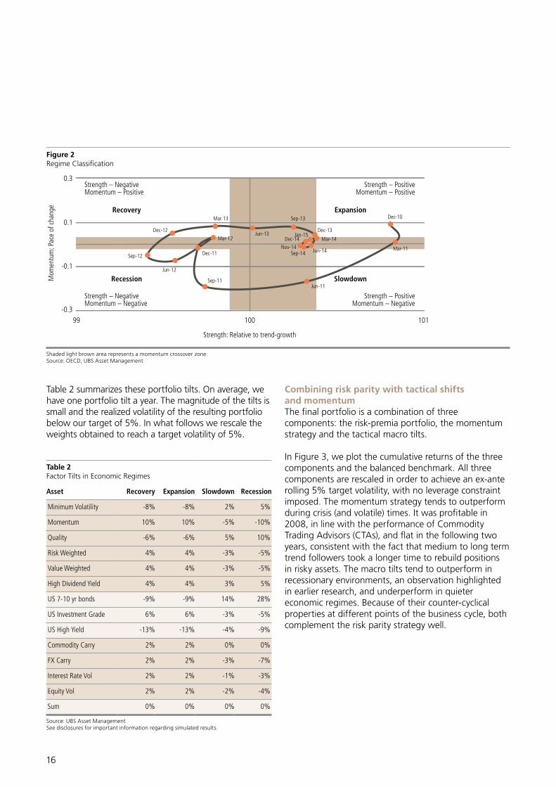
Introducing tactical tilts: The macroeconomic cycle and momentumThere is considerable evidence that asset returns or risk- premia are not constant through time, nor are correlations static. For instance, bear markets are characterized by high correlation across risky asset classes and a flight to quality. Observations like these have given rise to numerous studies on conditional asset allocation, whereby the composition of a portfolio depends upon the 'state' of the economy, or underlying risk regimes. It is beyond the purpose of this note to present a survey of these studies, but a few preliminary observations are necessary.

Generally, the time series predictability of these approaches has been found to be low but consistent with expectations, given the inherent difficulty of the task. However, in recent research Neely et al (2012)4 note that macroeconomic and technical indicators both tend to capture counter-cyclical information, but at different points of the cycle: Technical indicators tend to detect the typical decline in the equity risk premium near business cycle peaks while macroeconomic variables more readily pick up the typical rise in the equity risk premium later in recessions near cyclical troughs. This observation leads us to consider an approach that combines macro and technical based indicators.

The tactical tilts we propose are comprised of two components:

– A momentum strategy, including both cross-sectional and time series momentum, with a signal constructed over the previous 3, 6, 9 and 12 months with more emphasis on the longer time windows for stability

– A macro based strategy that applies fixed tilts to each asset based upon the state of the economy

Including momentum enables the capture of shifts that are typically not detected by fundamental variables, as well as identifying time-varying risk-aversion. In constructing the macroeconomic trading rule we use only one indicator, the OECD composite leading indicator (CLI), and classify the regime or state of the economy based upon two dimensions: (1) its 3-month rate of change and (2) its level.

Regime classification is done out of sample, using the latest available release each month. This indicator may be viewed as a base-case indicator given that there is a 2-month lag in the release of the latest data. Depending upon whether the economy is growing (e.g. positive 3-month change), and whether it is above average (e.g. level above 100), the regime is classified as being in recession, recovery, expansion or slowdown.

In order to address concerns over 'noise regime shifts' and its attendant portfolio turnover, we impose a 'no- change' band so that unless the indicator has crossed the 40% or 60% percentile (computed over past observations) we classify the current regime as being identical to the one the previous month. Figure 2 provides a graphical representation of how we classify regimes.5

During recessions, portfolio tilts are conservative. We overweight US government bonds and reduce allocation to high yield and investment grade. In equities, we increase the allocation to minimum volatility and quality while reducing momentum and the allocation to alternative beta. During recoveries, we tilt the portfolio in a more aggressive direction. Previous research suggests that tilts tend to be more successful in recessionary environments and that it may be difficult to distinguish between recoveries and expansion, or between slowdown and recessions. We simplify and assume less confidence for slowdown regimes (e.g. tilts are half than during recessions), and are identical during recoveries and expansions. This leaves us with three regime-dependent allocations.

3 We assume it to be 50% MSCI World and 50% WGBI. Returns are annualized and in excess of cash (i.e. US 3 month Libor).4 Neely, C.J., Rapach, D.E., Tu, J., Zhou, G, (2012), "Forecasting the Equity Risk Premium: The Role of Technical Indicators", Working paper, Federal Reserve Bank of St. Louis.5 Note that the graph, for ease of representation, is based upon the latest release whereas in the practice each data point pertains to its release date at the time.

16

Table 2 summarizes these portfolio tilts. On average, we have one portfolio tilt a year. The magnitude of the tilts is small and the realized volatility of the resulting portfolio below our target of 5%. In what follows we rescale the weights obtained to reach a target volatility of 5%.

Table 2Factor Tilts in Economic Regimes

Asset Recovery Expansion Slowdown Recession

Minimum Volatility -8% -8% 2% 5%

Momentum 10% 10% -5% -10%

Quality -6% -6% 5% 10%

Risk Weighted 4% 4% -3% -5%

Value Weighted 4% 4% -3% -5%

High Dividend Yield 4% 4% 3% 5%

US 7-10 yr bonds -9% -9% 14% 28%

US Investment Grade 6% 6% -3% -5%

US High Yield -13% -13% -4% -9%

Commodity Carry 2% 2% 0% 0%

FX Carry 2% 2% -3% -7%

Interest Rate Vol 2% 2% -1% -3%

Equity Vol 2% 2% -2% -4%

Sum 0% 0% 0% 0%


Combining risk parity with tactical shifts and momentumThe final portfolio is a combination of three components: the risk-premia portfolio, the momentum strategy and the tactical macro tilts.

In Figure 3, we plot the cumulative returns of the three components and the balanced benchmark. All three components are rescaled in order to achieve an ex-ante rolling 5% target volatility, with no leverage constraint imposed. The momentum strategy tends to outperform during crisis (and volatile) times. It was profitable in 2008, in line with the performance of Commodity Trading Advisors (CTAs), and flat in the following two years, consistent with the fact that medium to long term trend followers took a longer time to rebuild positions in risky assets. The macro tilts tend to outperform in recessionary environments, an observation highlighted in earlier research, and underperform in quieter economic regimes. Because of their counter-cyclical properties at different points of the business cycle, both complement the risk parity strategy well.

Figure 2Regime Classification

99 100

Slowdown

Dec-13

Sep-13

Jun-13

Mar-13

Dec-12

Sep-12

Jun-12

Mar-12

Dec-11

Sep-11Jun-11

Mar-11

Dec-10

Dec-14 Mar-14

Jun-14Sep-14Nov-14

Jan-15

101

Mom

entu

m: P

ace

of c

hang

e

0.3

0.1

-0.1

-0.3

Strength: Relative to trend-growth

Strength – NegativeMomentum – Negative

Strength – PositiveMomentum – Negative

Strength – NegativeMomentum – Positive

Strength – PositiveMomentum – Positive

Expansion

Recession

Recovery

Shaded light brown area represents a momentum crossover zoneSource: OECD, UBS Asset Management

17

Figure 3Cumulative Returns of the Strategy Components

-20

0

20

40

60

80

100

120

140

1989

Benchmark Risk parity

1994 1999 2004 2009 2014

Macro tilts Momentum


We form an aggregate portfolio by assigning 50% of the weight to the risk-parity portfolio, 25% to macro tilts strategy and 25% to momentum strategy. We constrain portfolio weights to be positive and gross leverage not to exceed 1. Because of these controls and the low correlation of the three components, the realized volatility of the portfolio falls just under 4%. In Table 3 we provide the summary statistics for three components and their combination in the final portfolio. Cumulative returns are shown in Figure 4.

Figure 4Cumulative Returns of Aggregate Portfolio

-0.2

-0.0

0.2

0.4

0.6

0.8

1.0

1989

Benchmark Combination

1994 1999 2004 2009 2014


Table 3Summary statistics

RiskPremia

MacroTilts

Mom-entum

Comb- ination

Sharpe 3 yrs 1.50 -0.17 1.23 1.47

5 yrs 1.53 0.10 0.86 1.46

10 yrs 0.86 0.46 1.33 1.18

since 1989 0.72 0.37 0.92 0.88

Avg Return (%) 4.24 2.09 5.21 3.36

Std Deviation (%) 5.86 5.73 5.63 3.84

Max Drawdown (%) -18.35 -17.95 -9.76 -5.40

Skewness -0.33 0.64 0.06 0.16

Kurtosis 5.07 6.20 6.44 4.64


The strategy exhibits flat returns in 2008 as losses in the core portfolio were offset by the gains in momentum and macro-based strategies. Momentum and risk-parity strategies achieve the highest risk-adjusted performance over the whole sample. As expected from a low-turnover strategy, the performance of the macroeconomic strategy is much weaker, especially in the last five years given that most of this time period was spent in recovery, a regime where tactical tilts tend to underperform. However this component has a 0% correlation with risk-parity and 30% with momentum, hence contributing to diversification. The combination exhibits a more stable risk-return profile through the entire sample and positive skewness5. Fat tails, as measured by kurtosis, are less pronounced. Finally, the ratio of maximum drawdown to standard deviation is more favorable.

We hope this note proves useful in two ways: First as a practical illustration of how factor risk-premia can be used in asset allocation, and second as example of how the conventional risk-parity approach can be enhanced by incorporating the momentum and macro-based strategies that lend diversification by adding value at different points in the market cycle.

5 Please note that Sharpe ratio and other statistics for the risk premia portfolio slightly differ from those in Table 1 because the portfolios in Table 3 have been rescaled to achieve an out of sample target volatility of 5%.

18

Your global investment challenges answeredDrawing on the breadth and depth of our capabilities and our global reach, we turn challenges into opportunities. Together with you, we find the solution that you need.

At UBS Asset Management we take a connected approach.

Ideas and investment excellence Our teams have distinct viewpoints and philosophies but they all share one goal: to provide you with access to the best ideas and superior investment performance.

Across markets Our geographic reach means we can connect the parts of the investment world most relevant for you. That’s what makes us different – we’re on the ground locally with you and truly global.

A holistic perspectiveThe depth of our expertise and breadth of our capabilities allow us to have more insightful conversations and an active debate, all to help you make informed decisions.

Solutions-based thinkingWe focus on finding the answers you need –and this defines the way we think. We draw on the best of our capabilities and insights to deliver a solution that’s right for you.

What we offerWe offer a comprehensive range of active and passive investment styles and capabilities, across both traditional and alternative asset classes. Our invested assets total CHF 633 billion and we have over 2,400 employees in 22 countries.

Who we areBacked by the strength of UBS, we are a leading fund house in Europe, the largest mutual fund manager in Switzerland and one of the largest fund of hedge funds and real estate managers in the world.

www.ubs.com/assetmanagement

Contact

Urs RaebsamenTel. +852 2971 7978

This document is for Professional Clients only. It is not to be distributed to or relied upon by Retail Clients under any circumstances. The views expressed are as of September 2016 and are a general guide to the views of UBS Asset Management. Comments are at a macro level and not with reference to any specific investment strategy or any registered or other mutual fund, or any other investment product or service. Please note that past performance is not a guide to the future. Potential for profit is accompanied by the possibility of loss. The value of investments and the income from them may go down as well as up and investors may not get back the original amount invested. This document is a marketing communication. Any market or investment views expressed are not intended to be investment research. The document has not been prepared in line with the requirements of any jurisdiction designed to promote the independence of investment research and is not subject to any prohibition on dealing ahead of the dissemination of investment research. This communication shall not be deemed to be an offer or the solicitation of an offer to buy any security or any investment product or service, nor shall any such security or investment product or service be offered or sold to any person in any jurisdiction in which such offer, solicitation, purchase or sale could be unlawful under the laws of such jurisdiction. The information and opinions contained in this document have been compiled or arrived at based upon information obtained from sources believed to be reliable and in good faith but no responsibility is accepted for any misrepresentation, errors or omissions. The details and opinions contained in this document are provided by UBS Asset Management without any guarantee or warranty and are for the recipient‘s personal use and information purposes only. All such information and opinions are subject to change without notice. A number of the comments in this document are based on current expectations and are considered “forward-looking statements”. Actual future results, however, may prove to be different from expectations. The opinions expressed are a reflection of UBS Asset Management’s best judgment at the time this document is compiled and any obligation to update or alter forward-looking statements as a result of new information, future events, or otherwise is disclaimed. Furthermore, these views are not intended to predict or guarantee the future performance of any individual security, asset class, markets generally, nor are they intended to predict the future performance of any UBS Asset Management account, portfolio or fund. Using, copying, redistributing or republishing any part of this document without prior written permission from UBS Asset Management is prohibited. Source for all data and charts (if not indicated otherwise): UBS Asset Management.

Additional disclosuresAustralian investors: This document is provided by UBS Asset Management (Australia) Ltd, ABN 31 003 146 290 and AFS Licence No. 222605. Hong Kong investors: The sole purpose of this document is purely intended for information to Professional Investors only (as defined in the Hong Kong Securities and Future Ordinance Cap571). Please note that the product(s) mentioned in this document is / are currently not authorized by the Securities and Futures Commission (the “SFC”) and not available for retail distribution in Hong Kong. Distribution of this document to the retail public is strictly prohibited. This document has not been reviewed by the SFC. Singapore investors: This document is solely for information and discussion purposes only and only intended for institutional investors as defined in section 4A of the Securities and Futures Act (Cap. 289) of Singapore. This document is not intended as an offer, or a solicitation of an offer, to buy or sell any investments or other specific product, and has not been recognised by the Monetary Authority of Singapore under the Securities and Futures Act (Cap. 289) for sale in Singapore. Services to U.S. persons are provided by UBS Asset Management (Americas) Inc. („Americas“) or UBS Asset Management Trust Company. Americas is registered as an investment adviser with the US Securities and Exchange Commission (“SEC”) under the Investment Advisers Act of 1940. From time to time, Americas’ non-US affiliates in the Asset Management Division who are not registered with the SEC („Participating Affiliates“) provide investment advisory services to Americas‘ U.S. clients. Americas has adopted procedures to ensure that its Participating Affiliates are in compliance with SEC registration rules. UK investors: This document is issued by UBS Asset Management (UK) Ltd and is intended for limited distribution to the clients and associates of UBS Asset Management. UBS Asset Management (UK) Ltd is a subsidiary of UBS AG. Registered in England and authorised and regulated by the Financial Conduct Authority. Telephone calls may be recorded. This document is a marketing communication. Any market or investment views expressed are not intended to be investment research. The document has not been prepared in line with the FCA requirements designed to promote the independence of investment research and is not subject to any prohibition on dealing ahead of the dissemination of investment research. Switzerland investors: This document has been issued by UBS AG, a company registered under the Laws of Switzerland. This commentary contains simulated results prepared by UBS Asset Management. The simulated results are presented for illustrative purposes only. Simulated results are developed with the benefit of hindsight and have inherent limitations. The analysis contained herein is based on historical analyses and numerous assumptions. Different assumptions could result in materially different results. The simulated results do not represent actual trading using client assets and are not based on the results of any actual strategy managed by UBS Asset Management. Investors should not take the example herein as an indication, assurance, estimate or forecast of future results. Actual results may differ materially from the simulated results shown. Simulated results may not reflect the impact that material economic and market factors might have had on UBS Asset Management decision making if actual client assets were managed during the time periods portrayed. No representation is being made that any strategy will achieve results similar to the simulated performance shown in this commentary. The simulated performance is presented gross of investment management fees. Actual returns would be reduced by advisory fees and other expenses incurred by the client. © UBS 2016. The key symbol and UBS are among the registered and unregistered trademarks of UBS. All rights reserved.

Alternative beta - UBS Global topics · Minimum expected tail loss ... alternative beta ... measure...

Documents

Transcript of Alternative beta - UBS Global topics · Minimum expected tail loss ... alternative beta ... measure...