ALTERNATIVE APPROACHES TO MEASURING THE COST OF EDUCATION William Duncombe1 John Ruggiero2 John Yinger1 1Center for Policy Research The Maxwell School Syracuse University 2Department of Economics and Finance University of Dayton Dayton, Ohio June 1995 Performance-Based Approaches to School Reform The Brookings Institution Washington, D.C., April 6-7, 1995.

ALTERNATIVE APPROACHES TO MEASURING THE COST OF EDUCATION Introduction

Over 20 years after the Serrano v. Priest (1971) decision by the California Supreme

Court sparked intense debate over school finance equity, the topic remains at the forefront of the

education reform debate in many states. Over the past two decades, a number of states have faced

law suits over the equity of their school finance system and several states have been forced to make

changes. In the last several years, a new round of court cases has challenged traditional equity

standards and solutions implemented in response to past court challenges. This paper addresses a

central issue in this debate, namely educational cost differences across school districts, that has

been virtually ignored by the courts and left out of recent reform efforts.

For the most part, the school finance debate has focused on differences in school district

fiscal capacity, and aid formulas typically make some effort to compensate low-capacity districts.

Much less attention has been paid to the other side of the school district budget, where cost

differences have a major impact on educational outcomes. The courts have focused on the

equalization of expenditure per pupil and not on adjusting expenditure to achieve equal educational

outcomes. Cost adjustments made by states tend to involve ad hoc adjustment factors, such as

"weighted pupil measures" to account for high-cost students and scale factors to compensate small,

rural school districts.1 Aid formulas based on these cost factors are likely to under-adjust for cost

differences, and indeed may even magnify existing disparities instead of easing them.

2

Over the last decade, several scholars have developed methods for constructing

educational cost indices. In this literature, the need to account for education cost factors is widely

acknowledged, but scholars disagree about the best way to define and measure costs. As we use

the term, "cost" refers to the expenditure or outlay needed by a district to provide a specified level

of education attainment or outcome, not to actual expenditure. In other words, cost refers to the

value of the resources a district must consume in the production of a given level of student

achievement. Cost differentials reflect both the costs of inputs and the harshness of the production

environment.2 Actual expenditure, on the other hand, reflects the influence not only of cost factors,

but also of demand factors, such as tax price, and of institutional factors.

Our objectives in this paper are to develop a method for estimating a comprehensive

district-level educational cost index that builds on the existing literature and can be implemented

with available data and then to estimate this index using data for New York State. Although we do

not explicitly consider state aid, methods for incorporating cost indices such as ours into state aid

formulas are well known.3 The main contribution of our approach is the development of new

methods to select educational outcome measures and to control for school district efficiency.

Moreover, the application to New York is instructive because school districts in the state have a

wide variety of educational environments, from sparsely populated rural areas to large central cities.

Our approach is consistent with many of the principles underlying recent educational reform

efforts. In particular, many states have moved from process-oriented to outcome-oriented policies,

3

such as the development of common standards and achievement measures. Moreover, many states

have implemented programs designed to encourage school choice and efficiency.4 Despite this new

focus, recent reform efforts have not recognized, for the most part, that outcomes and efficiency

cannot be accurately compared across districts without a viable method for measuring educational

costs. Some reforms, including those in South Carolina and Dallas, have discovered that

performance measures will be worse, on average, for low-income than for high-income schools and

make ad hoc adjustments to account for this cost-related effect.5 However, these reforms do not

explicitly recognize the role of input costs or environmental factors, and their adjustments do not

accurately account for cost variation across schools or school districts.

Our analysis shows how to estimate cost differences across districts controlling for district

efficiency, but a complete analysis of the role of cost indices in state aid formulas is beyond the

scope of this chapter, largely because district efficiency may be influenced by state aid. Moreover,

as many other chapters in this book make clear, education reform requires changes in incentive

systems and school management as well as in school finance. Our objective in this chapter is to

highlight the importance of educational cost differences across districts so that these differences can

be incorporated into broad school reform efforts. The cost models we develop can incorporate the

new performance measures which have been developed in recent education reforms.

4

Educational Production and Costs

Our approach builds on the large literature on educational production functions and

educational costs. This section reviews the key elements from this literature and discusses the

unique features of our approach. The following section presents our empirical analysis.

Educational Production Functions

The literature on the technology of public education focuses on a production function of the

form:6

(1) i t i ti t i t1 i i t = + + + + .S S eI Xα β δ µ

The subscripts i and t indicate school and time, respectively; S is a measure of educational service

or output, such as a test score or a drop-out rate; I is a vector of inputs, such as teachers and

classrooms; X is a vector of environmental factors, such as the share of students with learning

disabilities; e is a set of unobserved characteristics of the school and its pupils; µ is a random error

term; and a, ß, and d are parameters to be estimated.7 The lagged value of S captures the

continuing impact of inputs, environmental factors, and random errors in previous years on this

year's output; its coefficient, d, measures how fast the output from the previous year "deteriorates"

between school years.8

Environmental factors, X, also have been called "external" inputs, that is, inputs not

controlled by school officials. The term "environmental factors" is taken from the literature on local

5

public finance,9 whereas the term "external inputs" is taken from the literature on school production

functions. Although these two literatures developed separately, these two terms refer to exactly the

same concept. Several recent studies have brought these two strands of literature together.10

If observations for each school are available at three points in time, this equation can be

transformed into change form:

(2) i t i t1 i t i t1i t i t1 i t1 i t2 i t i , t1 = ( ) + ( ) + ( ) + ( ) .S S S SI I X Xα β δ µ µ

In this case, the dependent and explanatory variables are expressed in change form and the school-

specific effect, ei, cancels out. Without differencing, the unobserved school-specific effect can be a

source of omitted variable bias in equation 1.11

Focusing on a specific educational output is the most direct way to look at the technology

of public education. Moreover, this approach can be applied to school districts, schools,

classrooms, or even students.12 The more micro levels of focus make it possible to isolate the

variables that influence the interaction between students and teachers that is at the heart of this

technology.

This approach also has some disadvantages, however. The principal one for our purposes

is that it focuses on one output at a time.13 Public schools are complex institutions that provide

many different outputs, which are likely to share inputs and influence each other, that is, to be

produced jointly.14 As a result, it is difficult to make statements about the technology of production

6

for all educational outputs on the basis of equations 1 or 2. This limitation is crucial for us because

our objective is to determine the differences in technology, and the associated differences in costs,

for the unit that is evaluated and aided by state government, namely the school district. We need an

overview of educational technology in a district, not the specific classroom technology for a single

educational output.

Educational Cost Functions

This problem leads us to the principal alternative method for studying educational

technology, namely an analysis of school spending or costs, defined as the sum of input purchases.15

Associated with every production function, such as equation 1, is a cost function.

However, cost functions are only observed at the district level, in effect after the cost functions for

various educational outputs have been aggregated. Let the subscript j indicate the school district.

Suppose S* is an index of educational output for a school district, E is spending, and AC indicates

expenditure per unit of *jt-1S . Spending is measured in per pupil terms. Then by definition:

(3) *

j t j t j t = ( ) ( ) .S ACE

Moreover, a general form of the average cost function is (ignoring past history, Sjt-1 , for the

moment)

(4) *

j t j tj t j t j j t = c ( , , , , ) ,AC S P X ε ν

7

where P is a vector of input prices, e is a set of unobserved district-specific variables, and v is a

random error term. Combining equation 3 and equation 4 yields

(5) *

j t j t j tj t j j t = h ( , , , , ) .SE P X ε ν

Before estimating equation 5, we must deal with three major conceptual issues. The first

issue is that S* clearly is endogenous; school districts make spending and service quality decisions

simultaneously.16 Fortunately, the literature on the demand for public education provides extensive

instruments to use in a simultaneous equations procedure for equation 5. In particular, the standard

median voter model of education demand shows how public service quality, S* in our approach,

depends on income, intergovernmental aid, tax-share (usually specified as the ratio of median to

mean property values), and preferences.17

As an aside, this approach is based on the auxiliary equation

(6) *

j tj t j t = d ( , ) ,S D ψ

where D is a vector of demand variables and ? is a random error term. This equation can be

substituted into equation 5 to provide an alternative to our basic approach. Ultimately we will

compare cost indices based on equation 5 with cost indices based on equation 5 after equation 6

has been substituted into it. However, this "reduced form" approach has a major disadvantage

8

compared to estimating the structural equation 5, namely that environmental factors influence a

voter's tax price, which is her tax share multiplied by the marginal cost of public services, and

therefore are demand factors themselves. Hence, the coefficients of environmental variables in the

reduced-form approach reflect both their direct impact on educational costs, which is the effect we

are after, and their indirect impact through demand. These effects cannot be untangled without

assuming specific functional forms for the relationships in the modelCforms that cannot be tested.18

We prefer the structural approach because it requires no such assumptions.

The second issue concerns how to measure S*. One possible approach is to include every

possible measure of school outputs and let the regression procedure determine how they are

weighted to form S*. This approach has two serious problems. First, because output measures

often are highly correlated with each other, it introduces extensive collinearity into the regression.

This collinearity may make it impossible to estimate any coefficients with precision, including the

coefficients of the cost variables. Second, this approach undermines our ability to identify the

model, since every new (endogenous) output measure requires another instrument. As a practical

matter, therefore, the key problem is how to pare down the set of school output measures in a

sensible way.

Equation 6 provides a partial solution to this problem. When analyzing district spending,

one is interested in school output measures that households care about, as reflected in their demand

9

for public services. School output measures that are uncorrelated with demand variables do not fit

the bill.

This is only a partial solution to the problem, however, because equation 6 includes an error

term, ? , so that some outputs people care about at a district level may not be correlated with

demand variables, at least not with demand variables we can observe. Hence, evidence that an

output variable is correlated with demand variables must be combined with judgements about the

importance of various output measures based on previous literature. Our judgements on this issue

are presented below.

The third issue is that equation 5 includes two error terms, which we do not observe and

which might be a source of bias. The district-specific effect, e, which captures all unobserved

variables that do not vary over time, can be eliminated through differencing, as in equation 2.19 For

our purposes, however, differencing has two serious limitations. First, this procedure makes it

impossible to observe the impacts of input and environmental factors that do not vary over time;

these impacts are buried in the district-specific effect. Because many input and environmental

factors vary only slowly over time (and often cannot even be observed every year), this approach

may mask most of the variation in costs across districts and is not appropriate when one's objective

is to obtain a comprehensive cost index.

Second, as seen in equation 2, differencing does not eliminate variables that vary over time.

These variables are likely to include many inputs and environmental factors, along with unobserved

10

outputs, a district's past service quality, and its degree of inefficiency.20 Unless these variables are

accounted for, estimated coefficients for input and environmental factors that are included are likely

to be biased--even with differencing. Moreover, this bias could be upward or downward,

depending on the correlation between the included and excluded variables.

To deal with these problems, we estimate the undifferenced form of the cost function with a

new control variable designed to capture all the systematic components of both e and v. The

variable we use is based on a technique called Data Envelopment Analysis, or DEA, which has

been used to measure school district inefficiency21. Cost inefficiency is the extent to which a district

is spending more than necessary to obtain its output level. This inefficiency consists both of using

too many inputs for a given amount of output (technical inefficiency) and of using the wrong

combination of inputs given input prices (input allocative inefficiency). Further explanation of DEA

is provided in the appendix.

As it turns out, a standard DEA "efficiency" measure captures the impact of any factor that

influences the relationship between service quality and costs--not just district efficiency. All else

equal, an efficient district can obtain the same service quality as an inefficient district at a lower cost.

As discussed in the appendix, however, the relationship between service quality and costs is also

affected by environmental factors.22 Consider two equally efficient districts, one of which has a

very harsh environment compared to the other. The district with the harsher environment will have

to spend more to obtain the same service quality. Hence a standard DEA measure picks up the

11

impact of environmental factors as well as of efficiency. The same logic applies to any other

unobserved systematic factor in either error term of equation 5. Districts that made relatively high

investments in education in the past, for example, will have a favorable legacy that allows them to

obtain the same service quality as other districts at a lower cost.23

Thus, including a standard DEA "efficiency" measure will eliminate the potential bias from

the unobserved, and hence omitted, non-cost variables included in the two error terms in equation

5.24 DEA captures the impact of any factor that influences the relationship between service quality

and costs, so our DEA variable is a comprehensive insurance policy against omitted variable bias.

Unfortunately, however, this insurance policy has a price, namely the resulting duplication of

contemporaneous input and environmental cost variables.25 To be specific, input prices and

environmental factors are included as the Xs in equation 5 as well as in the DEA variable. As a

result, some of the full impacts of input prices and environmental factors on costs will be captured

by the estimated coefficients of the Xs and some will be captured by the DEA variable's coefficient.

We do not know exactly how these impacts will be divided, but we do know that the true impacts

will not be fully captured by the Xs, that is, by the observed values of the input prices and

environmental factors.

Our cost indices are based solely on the coefficients of the Xs and are not affected by the

coefficient of the DEA control variable. It follows that our approach inevitably provides an

12

underestimate of the impact of input prices and environmental factors on costs; some of the true

impact of the environment is buried in the DEA coefficient.

In addition, our approach focuses on the role of contemporaneous input prices and

environmental factors and ignores past values of these variables. One could argue that a cost index

should capture past as well as current values of these variables. A district should be compensated,

the argument might go, for the lingering effects of a relatively harsh environment in the past, as well

as for a harsh environment in the present. This argument has some appeal, but it also raises many

unresolved issues, such as how far back in history to go. Moreover, past history is difficult to

observe and incorporate into the model. To the extent that contemporaneous values of input prices

and environmental factors are highly correlated with past values, our approach may pick up some

past history. But neither our approach nor any previous research produces cost indices that include

a comprehensive treatment of each district's history of input prices and environmental variables.

In short, our approach provides a conservative estimate of the impact of contemporaneous

input prices and environmental factors on school district costs. Although an exact cost index would

be preferable, no procedure for estimating such an index is yet available, and our approach has the

advantage that the estimated coefficients are not biased upward (in absolute value) because of

unobserved district inefficiency or past effort. Moreover, a focus on contemporaneous, as opposed

to past, input prices and environmental factors, is appropriate given the complex role

(philosophically and technically) of past history and the limitations on available data.

13

One final point: A DEA "efficiency" measure also might be endogenous; that is, some of

the same factors that influence decisions about spending might also influence decisions that lead

districts to act in an efficient manner. To account for this possibility we identify an instrument for

district efficiency and treat the DEA measure as endogenous.

Cost Indices

For the purposes of designing intergovernmental aid formulas, one needs a measure of the

cost, based on factors outside a district's control, of providing a given quality of education.26

Educational quality is defined by the educational outputs, S. Because equation 5 determines the

impact of input and environmental costs on spending holding S constant, it is ideally suited for

calculating a cost index. This approach has been applied both for school and non-school

spending.27 Our cost indices are calculated in the same way as the indices in previous studies; as

explained below, these cost indices use the estimated regression coefficients to calculate the amount

each district would have to spend to obtain average quality public services.

An alternative approach to cost indices based on compensating wage differentials also has

appeared in the educational literature. According to this approach, some districts have to pay

higher wages than other districts to attract teachers of the same quality. Several studies have

estimated the extent to which teacher wages vary across districts based on factors outside a

district's control (accounting for factors that a district can control) and then calculated a wage index

based on this estimation.28

14

The problem with this approach is that it dramatically minimizes the role of the school

environment. A comprehensive cost index needs to account not only for the fact that some districts

must pay more than others to hire teachers of any given quality, but also for the fact that some

districts must hire more teachers than others to provide the same quality educational outputs for

their students. Indices based on wages alone therefore inevitably provide an incomplete and

potentially misleading picture of cost variation across districts.29 We will demonstrate this problem

using our New York data.

Empirical Analysis of Costs in New York School Districts

We estimate cost models and education cost indices for 631 school districts in New York

in 1991.30 This section describes our measures, data sources, and empirical analysis of education

costs, and it provides a comparison of alternative education cost indices.

Measures and Data Sources

Table 1 provides descriptive statistics for the variables used in the analysis. A district's

approved operating expenses (AOE) per pupil, which is provided by the New York State

Department of Education, is used to measure expenditure. AOE includes salaries and fringe

benefits of teachers and other school staff, other instructional expenditure, and all other expenditure

related to operation and maintenance of schools.31 Average AOE per pupil for the sample was

about $6,054.

15

Potential school outcome measures in our data range from standardized test scores to

dropout and graduation rates. Both the production and cost literature have relied most heavily on

average achievement test scores as output measures.32 A few studies also have emphasized the

role of test score distributions.33 One argument in favor of distributional measures, such as standard

deviations, is that education to some degree serves a screening function. As one scholar points out,

"In a screening model, the output of schools is information about the relative abilities of students.34

This would suggest that more attention should be directed toward the distribution of observed

educational outcomes (instead of simply the means)." Several studies also have focused on the high

school drop-out rate.

As discussed previously, collinearity severely limits the number of outcomes that can be

included in a cost model. We used a three-step process to select a reduced set of outcome

measures. First, we identified outcomes that appear to be related to voters' willingness to pay for

education by regressing each potential outcome measure on a set of education demand variables,

including income and tax share. Using a broad definition of "related," namely an adjusted R-

squared of at least 0.1, we were able to eliminate both the average and the standard deviation of

standardized achievement test scores as outcome variables for this analysis.35

Second, from the set of outcomes correlated with demand factors, we identified subsets of

variables that, based on previous research, appeared to be reasonable measures and then, where

appropriate, calculated an average across the variables in such a subset. This step led to three

16

outcome measures, all of which capture the tails of the student achievement distribution, instead of

the average as in much previous research. The first of these measures is based on Pupil Evaluation

Program, PEP, tests given to all third- and sixth-grade students in reading and math. The specific

measure is the average percentage of students performing above a standard reference point on

these four exams. The standard reference point is used to identify students requiring special

assistance (and Chapter 1 funding from the federal government). The second measure is the

percentage of students receiving a special Regents diploma upon graduation from high school.

Regents diplomas are given to students who pass standardized tests given by the state to high

school students. To balance this measure of achievement, the third measure is the inverse of the

drop-out rate, namely the percentage of students not dropping out of school.36

Third, we used factor analysis to determine whether the selection and clustering of our

outcome measures adequately captured the variation in the data across all potential such measures.

The size and pattern of the factor scores strongly supports our choices.37

As explained earlier, a cost model should control for unobserved district characteristics that

influence costs. Using the DEA method discussed in the previous section, a standard cost

"efficiency" index was constructed for each school district based on AOE per pupil and the three

outcome measures presented in Table 1. As explained earlier, this index captures not only

efficiency but also environmental cost factors and past school decisions that shift the cost frontier

facing a school district. Because this index is held constant in constructing the cost indices, we are

17

being conservative in our estimate of costs; that is, our cost indices ignore any cost effects picked

up by the DEA index instead of by the input and environmental variables in the cost model. The

average "efficiency" score is 0.66, with 23 districts (4 percent) with an index of one and 350

districts (55 percent) with an index below 0.7.

Cost differences across districts reflect both input price differences and environmental

factors. To measure input price differences, we estimated a teacher salary index. This index

adjusts for differences in teacher experience, education, and certification to reflect differences in the

cost of teachers of equivalent quality.38 A potential problem with the index is endogeneity arising

out of the relationship between teacher salaries and spending decisions.39 It is possible that some of

the variation in teacher salaries reflects discretionary decisions by district administrators, not

underlying differences in opportunity wages for teachers. To avoid this problem the index is based

on salaries of teachers with five years or less of experience. Even if excessive expenditures are

used primarily to increase teacher's salaries, this benefit is less likely to accrue to the most recently

hired teachers. Moreover, as explained below, this wage variable is treated as endogenous.

For the most part, the cost literature focuses on one environmental variable, namely the

number of students. The central question addressed in this literature is whether per-pupil costs rise

or fall when the number of pupils increase, that is, whether there are economies to pupil scale.40

Because many studies find that expenditures per pupil are a U-shaped function of enrollment, we

include enrollment and its square as environmental variables.41 Past studies have also considered

18

the share of students in secondary grades, the share of students in special education programs, the

share of students with limited English proficiency, and the share of students receiving a subsidized

lunch.42

The education production literature has highlighted the importance of family background

and student characteristics.43 Our data set allows us to measure several environmental variables in

these categories, namely the percentage of children in poverty, the percentage of households with a

female single parent, the percentage of children with limited English proficiency, the percentage of

students with a handicapping condition, and the percentage of total enrollment that is high school

students.44

Service outcomes, the efficiency index, and the price of labor are all determined

simultaneously with district spending through discretionary decisions made in the annual budgeting

process. To control for this endogeneity, our cost model is estimated using two-stage least squares,

with an appropriate set of additional instruments. The instruments associated with the service

outcomes are drawn from the literature on the demand for public services.45 Following a standard

median voter model, we use median income as a fundamental determinant of voter demand.

Demand also depends on intergovernmental aid; our state aid variable, basic operating aid, is the

principal form of non-categorical aid provided to school districts in New York.46 The standard tax

price facing the median voter equals her tax share multiplied by the marginal cost of educational

services. The marginal cost component is already in the cost model (in the form of the input price

19

and environmental factors), but the tax share makes a suitable instrument. We measure the tax

share with the ratio of median to mean residential property value and with an estimate of the

district's ability to export some commercial and industrial property taxes onto non-residents.47

Finally, we include several socio-economic variables that are likely to be related to demand for

education, namely the percentage of households with children, the percentage of households living in

owner-occupied housing, and the percentage of adults with a college degree.48

We also use instruments associated with the price of labor or the efficiency index. Since

comparable private sector prices for teachers were not available, we use 1990 county population

as a instrument for teacher salaries. Our choice of this instrument is based on the stylized fact (and

a central prediction of urban economics) that the cost of living, and hence, the cost of hiring

workers, increases with metropolitan population. Identifying instruments for the efficiency index is

more difficult. While there is a large literature on bureaucratic behavior, there is little associated

empirical literature examining the causes of inefficiency.49 The bureaucratic models suggest that

greater inefficiency will be associated with larger and wealthier school districts, those facing less

competition, and those with poorer performance incentives for their employees. Enrollment and

median income already have been included as exogenous variables. Good measures of private

school competition are not available, but competition also may come in the form of voter referenda

on school budgets. In New York, all school districts are required to have budget referenda except

20

for city school districts, where the budget is set entirely by elected city officials. A dummy variable

for city districts therefore is included as an instrument for the efficiency index.50

Cost Model Results

We estimate our education cost models using a modified Cobb-Douglas cost model with a

quadratic enrollment term. The Cobb-Douglas form imposes several restrictions on the production

technology for educational services.51 The simplicity and conceptual plausibility of this function

along with its frequent successful application in empirical research outweigh its potential limitations.52

The dependent variable is the log of AOE per pupil. The cost models were estimated using linear

2SLS, with outcome measures, the efficiency index, and the price of labor treated as endogenous.

Our initial specification, called Model 1, is presented in the first column of Table 2. This

specification, which is based on the three outcome measures defined above, performs very well.

The outcome measures all have positive coefficients, as expected, and two of the three coefficients

are statistically significant. The PEP test scores variable (the average percentage of students above

standard reference point) has a t-statistic of 1.5. The Aefficiency@ index has, as expected, a

negative coefficient and is statistically significant; greater efficiency in a school district is associated

with lower expenditure, ceteris paribus.

Moreover, six of the eight cost variables have statistically significant coefficient with the

expected signs. The teacher salary variable is, as expected, positively related to expenditure and its

coefficient is quite large; in fact, a 1.0 percent increase in teacher salaries is associated a 0.89

21

percent increase in per pupil expenditure. Both enrollment variables are statistically significant and

indicate a U-shaped per pupil expenditure function. Based on these results, the "minimum cost

enrollment" falls at a district enrollment of about 3,300 pupils.53 Child poverty rates and the

percentage of female headed households, included to reflect family background, are both positively

related to expenditure and statistically significant, and we find a positive and significant relationship

between spending and the share of high school students with limited English proficiency. The

percentage handicapped and percentage high school variables also have the expected signs but their

t-statistics are just above 1.0. Overall, this regression provides strong confirmation of our

approach; by controlling for (endogenous) outcome measures, efficiency, and past history, one can

precisely measure the impact of many contemporaneous input and environmental cost variables on

school district spending.

We also estimated several variants of this model to determine the robustness of our results.

In Model 2 we explore one possible explanation for the insignificance of the percentage

handicapped variable, namely the heterogeneity of the students in this category and the associated

variation in the special services they need. Using disaggregated information on handicapped

students in New York by the level of service then receive, we examined several handicapped

variables in the cost model.54 The percent of students with severe handicapping conditions

(requiring special services out of the regular classroom at least 60 percent of the school day) does

have a statistically significant positive affect on district expenditures. A one percentage point

22

increase in these students raises per pupil expenditures by close to one percent. The other outcome

and cost factors remain statistically significant with little change in their coefficients. Model 2 is our

preferred specification and is used to construct our principal cost index in Tables 3 and 4.

Because one of our outcome measures is not statistically significant, we also estimated cost

models using two different pairs of outcome measures. The resulting models, called Models 3 and

4 in Table 2, each include a DEA efficiency index based on only the two outcome measures in the

model. In both cases, the coefficient of the PEP scores variable is statistically significant with a

magnitude similar to that in Model 1. These results reinforce the importance of controlling for

elementary student performance in the construction of cost indices and suggest that it may be

collinearity that keeps down the significance of the PEP variable in Models 1 and 2. Because it

provides a broader range of outcome measures, we will utilize the three-outcome model to

construct our education cost indices.

Comparison of Education Cost Indices

The cost models in Table 2 can be used to construct comprehensive educational cost

indices. Our cost index is designed to capture the key cost factors outside of a district's control,

including the underlying cost of hiring teachers (the opportunity wage), district size, family

background, and student characteristics. Variation in expenditure among districts that reflects

differences in service quality, in efficiency, or in past history is eliminated from the calculations; that

is, service quality and efficiency are held constant across districts. To be specific, we multiply

23

regression coefficients by actual district values for each cost factor (and by the state average for

outcomes and efficiency) to construct a measure of the expenditure each district must make to

provide average quality services given average inefficiency.55 Our cost indices simply express this

predicted expenditure relative to the state average.56

The first column of Table 3 presents our principal cost index, which is based on Model 2 in

Table 2. This index has a range from 78 to 240 with a standard deviation of 17. Seventy-five

percent of the districts have indices below 105, and 75 percent have indices above 90.

Table 3 also presents several alternative cost indices. Columns 2 and 3 presents cost

indices based on alternative cost models; the cost model in column 2 has no control for district

Aefficiency,@ and the one in column 3 treats district efficiency as exogenous. These columns reveal

that, compared to our preferred model, ignoring Aefficiency@ tends to magnify cost differences

across districts whereas treating Aefficiency@ as exogenous tends to dampen them. Because our

Aefficiency@ index reflects cost factors to some degree, leaving out this index boosts the impact of

the cost factors in the equation. Because the index also reflects other factors, such as efficiency,

that may be correlated with costs, the index in column 2 may be affected by omitted variable

biasCand may therefore overstate cost differences across districts. Treating efficiency as

exogenous introduces another possible bias, namely endogeneity bias. As it turns out, the effect of

leaving out the Aefficiency@ variable altogether is smaller than treating Aefficiency@ as exogenous, at

least on average, so the correlation between the indices in the first two columns, 0.94, is higher than

24

the correlation between the indices in columns one and three, 0.84. This result indicates that a cost

index correcting for Aefficiency,@ which is difficult to obtain, is roughly proportional to a cost index

without an Aefficiency@ correction. However, the actual distribution of aid using these two cost

indices be quite different because the Aefficiency@ correction lowers variation in costs.

Table 3 also compares our preferred cost index with a cost index based on an alternative

approach in the education literature and with two forms of cost indices widely used in practice. As

explained earlier, if demand variables are substituted for service outcomes, then an indirect (or

reduced-form) expenditure model can be used to construct a cost index.57

Most states use some form of weighted pupil measure in the allocation of aid. In New

York, for example, students with special needs, handicapping conditions, or in secondary school

receive heavier weights in the distribution of aid. By taking the ratio of weighted pupils (specifically,

total weighted pupil units, TWPU) to total enrollment we construct a cost index that indicates the

level of cost adjustment in a typical state aid formula. This approach makes ad hoc adjustments for

cost differences across some types of students and is likely to understate overall cost differences

because it focuses on only a few cost-related student characteristics.

The most common cost index proposed in education research focuses on the relationship

between socio-economic factors and teacher salaries. Teachers are expected to command higher

salaries if they are of higher quality (or have characteristics rewarded in union contracts), or if they

have to work under more adverse working conditions. Working conditions can be affected by

25

district decisions concerning resource utilization (pupil-teacher ratios) or by socio-economic factors

out of the district's control that reflect the harshness of the education environment (such as a

relatively high incidence of special needs or disadvantaged children). By holding teacher quality,

demand variables, and discretionary resource factors constant, these studies have constructed

education cost indices to reflect the wage differentials required to "compensate" for an adverse

socio-economic environment.58 While a compensating wage-based cost index may capture cost

factors associated with higher teacher salaries, it does not control for differences across districts in

resource usage (including hiring of teachers!) required to provide a given level of service outcomes.

The last three columns of Table 3 present these alternative education cost indices. The

indirect cost index, which does not control for inefficiency has slightly lower variability than our

preferred cost index in column 1.59 The least variability appears in the weighted-pupil and teacher-

salary indices, largely because these indices are only capturing a portion of actual cost differentials.

Correlation coefficients reiterate the substantial differences among these indices. The

correlation between our preferred index and the indirect index is 0.63, which suggests that the

indirect approach may not do a good job controlling for service quality differences and may

therefore result in biased cost indices.60 The correlation between our preferred index and the

weighted-pupil index is extremely low, only 0.14; the approach used by New York State therefore

misses most of the actual variation in costs across districts. Finally, the correlation between our

preferred index and the teacher salary index is 0.47, indicating only a moderate correlation between

26

the factors that push up the salary needed to attract a given quality of teacher and the factors that

push up the cost of providing a given quality of educational services. The teacher salary index is not

related to either the indirect cost index or the weighted pupil index.

To provide a more disaggregated comparison of these cost indices, Table 4 presents

average index scores by region, enrollment size, and income and property wealth of school districts.

The direct cost index with endogenous efficiency identifies the large upstate central cities and

downstate small cities as having the highest costs. (The large downstate cities, New York City and

Yonkers, are not included in sample due to missing data.) This result reflects higher teacher salaries

in downstate districts and higher environmental cost factors in upstate cities. Upstate suburbs and

rural districts have below average costs. This table also clearly shows the U-shaped relationship

between costs and enrollment and reveals that costs tend to be slightly higher for both the poorest

and the richest districts, measured by either income or property wealth. Higher income or wealth

districts, particularly in downstate New York, may have a relatively favorable educational

environment, but they must pay relatively high teacher salaries.

Table 4 also shows the values for the alternative indices in each of these categories.

Compared to our preferred index, the cost differences across types of district are magnified

somewhat with the no-efficiency index and dampened considerably with the weighted-pupil,

teacher-cost and indirect cost indices. Comparing the various indices by pupil-size category

reinforces the similarity between our preferred index and the no-efficiency index, but also reveals

27

substantial differences between our preferred index and the others. The indirect cost index

accentuates the U-shaped relationship between enrollment and per pupil costs, while the other

indices understate this relationship. In general, they completely fail pick up the relatively high costs

of small districts and understate the costs of the largest districts.61 Comparisons based on income

class or property value class also identify several distinct differences between indices. While our

preferred index shows little variation across income (and property wealth) classes, the no-

efficiency, indirect cost, and teacher salary indices show substantially higher costs in low-income

districts. These differences are difficult to interpret since they could reflect either inefficiency or

unobserved environmental cost factors.

What types of districts tend to have particularly high or low costs and which environmental

factors principally account for these cost differences? To answer this question we examined the ten

percent of school districts with the highest and lowest costs (Table 5). Average values for

environmental factors for these districts are compared to the state average. For high-cost districts,

costs average 52.7 percent above the state average, $3,046 per pupil. All upstate large cities and

over 70 percent of downstate small cities qualify as high-cost districts. Over 10 percent of

downstate suburbs and upstate small cities also fall in this category. Enrollment, percent of children

in poverty and with limited English proficiency, and percent of single-parent female-headed

households are all well above the state average in these districts.

28

Combining the environmental indices with the regression coefficients for model 2 in Table 2,

we can identify which environmental factors have a particularly strong effect on costs. Higher

teacher salaries and a relatively high number of female-headed households each account for over 30

percent of the higher costs in these districts. Limited English proficiency and poverty are also

important factors driving up costs. The higher enrollments in some high-cost districts may actually

lower per pupil costs, because their enrollments are close, on average, to the cost minimizing

enrollment.

The 10 percent of districts with the lowest costs have costs 20 percent below average,

$1,091 per pupil. Most of these districts are upstate suburbs; a few are rural districts. Poverty,

female-headed households, severely handicapped students, and students with limited English

proficiency are all relatively uncommon. Lower teacher salaries, lower poverty rates, fewer female-

headed households, and higher enrollments each account for 20 percent of the lower costs in these

districts.

29

Conclusions and Policy Implications

At the conceptual level, the importance of educational costs cannot be denied. Through no

fault of their own, some school districts must spend more than other districts to obtain the same

level of educational outcomes. Despite widespread agreement on this point among scholars,

educational cost indices remain illusive because any method to estimate them must overcome

complex methodological obstacles. Given the stakes involved, namely the allocation of state

educational aid, we believe that overcoming these obstacles is one of the principal challenges facing

scholars and policy makers interested in education finance. This paper develops and implements a

method for estimating educational cost indices that resolves some of these difficulties.

Our approach, like several others, focuses on the impact of input prices and environmental

cost factors on educational spending, controlling for educational service quality. This approach

leads to an index of the amount a school district would have to spend, given the input prices and

environment it faces, to obtain average-quality educational services. Our contributions are to

develop new criteria for selecting service quality measures and to explicitly control for school

district efficiency and other unobserved district characteristics that might lead to biased cost indices.

When applied to data for school districts in New York state, our approach works well in

the sense that most of the regression coefficients are statistically significant and all of them have the

anticipated signs. Hence, the cost indices we estimate control for a variety of service quality

measures (as well as district efficiency) and estimate with precision the impact of input prices and

30

environmental factors on educational costs. The major disadvantage of our approach is that it

requires the calculation of a complex "efficiency" measure, based on Data Envelopment Analysis.

This disadvantage may make our approach impractical as a tool for designing school aid formulas.

We also find, however, that cost indices based on a cost model that does include the DEA

index are highly correlated with those based on our preferred cost model. Thus, school aid

formulas based on this simpler formula might be acceptable. However, a better compromise would

be to discover simpler methods to control for district efficiency and other unobserved district

characteristicsCand to include these methods in a cost model. We also find two widely used

methods for estimating educational costs, namely those based on weighted pupils and on required

teacher salaries, do not provide reasonable approximations for our method, which is to be

preferred on conceptual grounds. The weighted-pupil cost index used in New York is virtually

uncorrelated with our cost index, and the teacher-salary index is only moderately correlated, misses

the U-shaped relationship between costs and enrollment, and greatly understates the costs in large

city districts. In our judgement, therefore, these approaches are seriously deficient.

Educational cost variation across school districts is a crucial issue that has not been

adequately recognized by either courts or state legislatures. Despite its fundamental consistency

with a focus on school performance, it also has not been adequately incorporated into recent

performance-based school reform efforts. The large literature on production and cost in education

provides a solid foundation for the development of education cost indices. This paper demonstrates

31

the serious flaws in existing ad hoc indices, which do not build on this foundation, and shows how

more acceptable cost indices can be derived.

32

APPENDIX Measuring Inefficiency in Public Services

Several methods for estimating technical and cost efficiency have been developed over the

last several decades. The non-parametric method used in this paper, Data Envelopment Analysis,

DEA, is based on production theory in economics and has been operationalized as DEA since the

laste 1970s.62 One of the major advantages of DEA is that it is non-parametric, that is, it requires

no a priori specification of the functional form. One disadvantage is that the technique is non-

stochastic.63

These methods have been extended to analyze costs and economies of scope in public

sector production. The relevant mathematical programs are solved to compare the expenditure of a

given local government with the expenditure of other local governments producing the same level of

services. If the local government is producing at the cost-minimizing level, then no other local

government (or linear combination of local governments) is producing the same level of services

with lower expenditure.64

One problem with existing DEA methods for estimating inefficiency is the maintained

assumption that the technology can be represented by one frontier. This assumption presumes that

all deviations from the cost frontier are attributable to inefficiency. While DEA has been commonly

employed to examine public organizations such as school districts, the assumption of one cost

frontier is not consistent with the nature of public production.65 As explained in the text, input

33

prices, P, and exogenous socio-economic variables, X can have an important influence on the

translation of government activities into service outcomes. As a result, there will be multiple cost

frontiers reflecting differences in P and X. Estimates of the minimum level of costs and cost

inefficiency that do not control for these cost factors will be biased.

Recently, a method has been developed for estimating technical and cost efficiency that

allows for multiple frontiers.66 Figure 1 illustrates two minimum cost frontiers assuming for simplicity

one service outcome, S. For all levels of S, C(S|P1, X0) $ C(S|P0, X0) because P1 >P0. Efficiency

estimates should be made in reference to the correct frontier. A local government is said to be cost

efficient if the observed level of expenditure is equal to the minimum total cost of providing the

observed level of services, given resource prices and environmental conditions.

While this method provides a more realistic estimate of relative cost efficiency among

school districts, it can handle only a few fixed cost factors, and these fixed cost factors must be

selected prior to estimation of the cost model. Selected cost factors may turn out to be statistically

insignificant, so that a complex iterative procedure would have to be developed to make the

regression and the DEA consistent. To avoid these problems, we use the unadjusted cost efficiency

index, which compares all districts to the cost frontier for the district with the most favorable

environment. Specifically, our measure of cost "efficiency," ?, is equal to C/E, where C equals

minimum costs and E equals actual expenditure.

If local governments are cost efficient and face the most favorable cost environment, then expenditure reflects the minimum cost of providing services and ? equals 1.0. In any other case,

34

that is, with either inefficiency or unfavorable fixed factors, ? is less than 1.0. To illustrate, assume P0 and X 0 in Figure 1 represent the most favorable educational environment (minimum cost frontier for district I). The cost efficiency index for district H would be ?H = C(S|P0, X 0)/E H. Since district H faces higher factor prices, C(S|P1, X0)/EH represents the true (unobserved) cost efficiency and C(S|P1, X0)/C(S|P0, X0) the index of environmental harshness.

35

Endnotes

1. For a good discussion of past court challenges see Allan Odden and Lawrence Picus, School

Finance: A Policy Perspective (McGraw-Hill, Inc., 1992). Steven Gold, David Smith, Stephen

Lawton, and Andrea C. Hyary, Public School Finance Programs of the United States and

Canada, 1990-91 (The Nelson A. Rockefeller Institute of Government, 1992) provide a good

overview of state aid systems in the early 1990s.

2. See Helen Ladd and John Yinger, AThe Case for Equalizing Aid,@ National Tax Journal, 47

(March 1994), pp. 211-224.

3. See Ladd and Yinger, AThe Case for Equalizing Aid,@ pp. 211-224, for an overview of adding

costs to several types of aid formulas.

4. For general discussion of education reform and school choice, see Susan Fuhrman, Richard

Elmore, and Diane Massell, ASchool Reform in the United States: Putting it into Context,@ in S.

Jacobson and R. Berne, eds., Reforming Education: The Emerging Systemic Approach

(Thousand Oaks, CA: Corwin Press, Inc., 1993), Bruce Cooper, AEducational Choice: Competing

Models and Meanings,@ in S. Jacobson and R. Berne, eds., Reforming Education: The Emerging

Systemic Approach (Thousand Oaks, CA: Corwin Press, Inc., 1993), and Eric Hanushek,

Making Schools Work: Improving Performance and Controlling Costs (The Brookings

Institution, 1994).

36

5. See C. Clotfelter and Helen Ladd, APicking Winners: Recognition and Reward Programs for Public

Schools,@ this volume.

6. This literature is reviewed in Eric Hanushek, AThe Economics of Schooling: Production and

Efficiency in Public Schools,@ Journal of Economic Literature 24 (1986), pp. 1141-1177,

Elchanan Cohen and Terry Geske, The Economics of Education (Pergamon Press, 3rd edition,

1990), and David Monk, Educational Finance: An Economic Approach (McGraw Publishing

Company, 1990).

7. This error structure assumes that the error component, e, does not vary over time. This assumption

may not be appropriate if the error component includes student cohort effects as well as school

effects. For simplicity, this equation is written in linear form, although other forms can be used.

8. The concept of service "deterioration" is discussed at length in the chapter by Ronald Ferguson and

Helen Ladd, AAdditional Evidence on How and Why Money Matters: A Production Function

Analysis of Alabama Schools,@ this volume. Note that the specification with a lagged value of S

also can be derived by including lagged values of I, X, and µ and then subtracting the equations for

two succeeding years. With this approach, the coefficients for the lagged values of I and X must

"deteriorate" over time at the same rate such that ßt-i = dißt, where ß t is the coefficient vector for

these variables in year t.

37

9. David Bradford, Robert Malt and Wallace Oates, AThe Rising Cost of Local Public Services: Some

Evidence and Reflections,@ National Tax Journal 22 (June 1969), pp. 185-202; Katherine

Bradbury, Helen Ladd, Mark Perrault, Andrew Reschovsky, and John Yinger, AState Aid to Offset

Fiscal Disparities across Communities,@ National Tax Journal 37 (June 1984), pp. 151-170; and

Helen Ladd and John Yinger, America's Ailing Cities: Fiscal Health and the Design of Urban

Policy (The Johns Hopkins University Press, 1991).

10. These studies include Kerri Ratcliffe, Bruce Riddle, and John Yinger, AThe Fiscal Condition of

School Districts in Nebraska: Is Small Beautiful?@ Economics of Education Review 9 (1990), pp.

81-99; Richard Fenner, The Effect of Equity of New York State's System of Aid for Education,

Ph.D dissertation, Syracuse University, 1991; and Thomas Downes and Thomas Pogue, AAdjusting

School Aid Formulas for the Higher Cost of Educating Disadvantaged Students,@ National Tax

Journal 47 (March 1994), pp. 89-110.

11. Because this step also requires at least three years of data, it has not been taken by any production

function study of which we are aware. The excellent chapter by Ferguson and Ladd, AAdditional

Evidence on How and Why Money Matters: A Production Function Analysis of Alabama

Schools,@ for example, is based on one of the most complete data sets in the literature, but it

estimates equation (1), not equation (2).

12. As pointed out by Summers and Wolfe and Hanushek, among others, in applying this model to

38

individual students one must distinguish between individual and family background variables, peer-

group variables, and school variables. See Anita Summers and Barbara Wolfe, ADo Schools Make

a Difference?@ American Economic Review, 67 (September 1977), pp. 639-652; and Eric

Hanushek, AConceptual and Empirical Issues in the Estimation of Educational Production

Functions,@ The Journal of Human Resources, 14 (1979), pp. 351-388.

13. Another disadvantage is that extensive data are required.

14. Multi-product production functions have typically assumed separability between outputs so that

each can be estimated in a separate equation (possibly allowing correlation across error terms by

using a seemingly unrelated regression method). On the other extreme, some studies (Boardman,

Davis, and Sanday) in the public sector have estimated simultaneous production functions which

assume that each output simultaneously influences the other. If the production of outputs share

some inputs but do not necessarily cause each other, then a production function which allows for

jointness of production is the most appropriate. Recently, canonical regression has been used to

estimate joint production functions. However, no one has yet shown how to use this approach to

develop comprehensive educational cost indices. See Anthony Boardman, Otto Davis, and Peggy

Sanday, AA Simultaneous Equations Model of the Education Process,@ Journal of Public

Economics, 7 (1977), pp. 23-49; John Chizmar and Thomas Zak, AModeling Multiple Outputs in

Educational Production Functions,@ American Economic Review, 73 (May 1983), pp. 18-22;

39

Kwabena Gyimah-Brempong and Anthony Gyapong, ACharacteristics of Education Production

Functions: An Application of Canonical Regression Analysis,@ Economics of Education Review,

10 (1991), pp. 7-17; and John Ruggiero, AMeasuring Technical Inefficiency in the Public Sector:

An Analysis of Educational Production,@ Review of Economics and Statistics, forthcoming, 1995.

15. Recent examples of this approach include Downes and Pogue, AAdjusting School Aid Formulas for

the Higher Cost of Educating Disadvantaged Students,@ pp. 89-110; Kwabena Gyimah-Brempong

and Anthony Gyapong, AElasticities of Factor Substitution in the Production of Education,@

Economics of Education Review, 11 (1992), pp. 205-217; Fenner, The Effect of Equity of

New York State's System of Aid for Education; Scott Callan and Rexford Santerre, AThe

Production Characteristics of Local Public Education: A Multiple Product and Input Analysis,@

Southern Economic Journal, 57 (October 1990), pp. 468-480; Ratcliffe, Riddle, and Yinger,

AThe Fiscal Condition of School Districts in Nebraska: Is Small Beautiful?@. Earlier studies are

reviewed in Cohen and Geske, The Economics of Education, and Monk, Educational Finance:

An Economic Approach.

16. Despite the obvious endogeneity of service quality, we know of only two studies of educational

costs that treats service quality as endogenous, namely Baum, and Downes and Pogue. See

Donald Baum, AA Simultaneous Equations Model of the Demand for and Production of Local

Public Services: The Case of Education,@ Public Finance Quarterly, 14 (1986), pp. 157-78; and

40

Downes and Pogue, AAdjusting School Aid Formulas for the Higher Cost of Educating

Disadvantaged Students,@ pp. 89-110.

17. For a detailed discussion and literature review on these issues, see Ladd and Yinger, America's

Ailing Cities: Fiscal Health and the Design of Urban Policy (The Johns Hopkins University

Press, 1991). The specific instruments we use are presented below.

18. This point is made by Schwab and Zampelli, and Downes and Pogue. A detailed exposition of the

necessary structure is provided in Ladd and Yinger. One important assumption that is required to

identify cost parameters in a reduced-form model is constant returns to scale with respect to

changes in S*. See Duncombe and Yinger for a detailed discussion of this point. See Robert

Schwab and Ernest Zampelli, ADisentangling the Demand Function from the Production Function

for Local Public Services: The Case of Public Safety,@ Journal of Public Economics, 33 (1987),

pp. 245-260; Downes and Pogue, AAdjusting School Aid Formulas for the Higher Cost of

Educating Disadvantaged Students,@ pp. 89-110; Ladd and Yinger, America's Ailing Cities:

Fiscal Health and the Design of Urban Policy; William Duncombe and John Yinger, AAn

Analysis of Returns to Scale in Public Production, With an Application to Fire Protection,@ Journal

of Public Economics, 52 (1993), pp. 49-72;

19. A first-differencing approach is used by Downes and Pogue, AAdjusting School Aid Formulas for

the Higher Cost of Educating Disadvantaged Students,@ 89-110. They are aware of the fact that

41

differencing eliminates some cost variables and explicitly develop cost indices only for two cost

variables, namely the factions of students receiving subsidized lunches and with limited English

proficiency.

20. Hanushek points out that inefficiency may make it appear that "expenditures are unrelated to school

performance." Ruggiero found evidence that inefficiency dampens the observed impact that school

inputs have on outputs. See Eric Hanushek, AThe Economics of Schooling: Production and

Efficiency in Public Schools,@ pp. 1166; Ruggiero, AMeasuring Technical Inefficiency in the Public

Sector: An Analysis of Educational Production.@

21. See, for example Shawna Grosskopf and S. Yaisawarng, AEconomies of Scope in the Provision of

Local Public Services,@ National Tax Journal, 43 (1990), pp. 61-74; and John Ruggiero, AAre

Costs Minimized in the Public Sector? A Nonparametric Analysis of the Provision of Educational

Services,@ Metropolitan Studies Program Occasional Paper No. 165, Center for Policy Research,

The Maxwell School (Syracuse, NY: Syracuse University, 1994).

22. Ruggiero has shown how to measure inefficiency controlling for the environment in a DEA

framework through the use of multiple cost frontiers (see the appendix). As explained below,

however, this solution is not appropriate here. See Ruggiero, AAre Costs Minimized in the Public

Sector? A Nonparametric Analysis of the Provision of Educational Services.@

42

23. Downes and Pogue account for past history by including both 12th-grade test scores and 11th-

grade test scores for the same cohort. This is analogous to the service-quality term on the right side

of equation 2, and picks up the history of cost factors, as well as of other variables. See Downes

and Pogue, AAdjusting School Aid Formulas for the Higher Cost of Educating Disadvantaged

Students,@ pp. 89-110.

24. One important criticism of DEA is that the outputs on which it is based are selected by the

researcher, not by some statistical test. This criticism does not apply to our equations because the

outputs used in the DEA procedure are the same ones used in equation 5, where a statistical test of

their significance is provided. See Hanushek, AThe Economics of Schooling: Production and

Efficiency in Public Schools,@ pp. 1141-1177.

25. In principle, one could avoid this duplication by using the Ruggiero procedure to correct for

environmental cost factors. However, this approach is not practical here because, as explained by

Ruggiero, DEA cannot handle as many cost factors as are required for our procedure without a

much larger sample of school districts than exists in any state, including New York. See Ruggiero,

AAre Costs Minimized in the Public Sector? A Nonparametric Analysis of the Provision of

Educational Services.@

26. For a detailed discussion of the use of cost indices in education formulas, see Ladd and Yinger,

43

AThe Case for Equalizing Aid,@ pp. 211-224.

27. For non-school spending see Bradbury et al., AState Aid to Offset Fiscal Disparities across

Communities,@ pp. 151-170, and Ladd and Yinger, America's Ailing Cities: Fiscal Health and

the Design of Urban Policy. And for school spending see Ratcliff, Riddle, and Yinger AThe Fiscal

Condition of School Districts in Nebraska: Is Small Beautiful?@ and Downes and Pogue, AAdjusting

School Aid Formulas for the Higher Cost of Educating Disadvantaged Students.@

28. See, for example, Jay Chambers, AEducational Cost Differentials and the Allocation of State Aid

for Elementary and Secondary Education,@ Journal of Human Resources, 13 (1978), pp. 459-

481; Jay Chambers, AThe Development of a Cost of Education Index: Some Empirical Estimates

and Policy issues,@ Journal of Education Finance, 5 (Winter 1980), pp. 262-281; Howard

Fleeter, ADistrict Characteristics and Education Costs: Implications of Compensating Wage

Differentials on State Aid in California,@ mimeo (Ohio State University, 1990); and Wayne

Wendling, AThe Cost of Education Index: Measurement of Price Differences of Education

Personnel among New York State School Districts,@ Journal of Education Finance, 6 (Spring

1981), pp. 485-504.

29. Monk and Walker (p. 174) argue that a more comprehensive approach "presupposes an ability to

reach agreement about the nature and level of outcomes schools are expected to produce." We

agree that one must select output measures in order to implement equation 5, but we think that

44

reasonable procedures can be developed for making this selection. Moreover, the fact that a step

may be difficult is a poor excuse for not attempting it, particularly when the conceptual case for it is

so strong. Finally, one can estimate cost indices without selecting output measures if one substitutes

equation 6 into equation 5. See David Monk and Billy Walker, AThe Texas Cost of Education

Index: A Broadened Approach,@ Journal of Education Finance, 17 (Fall, 1991), pp. 172-192.

30. There were 695 school districts in New York in 1991. Due to missing observations (including

New York City and Yonkers), the sample was limited to 631 observations. The remaining sample

appears representative of the major regions in New York State.

31. This measure of expenditure excludes transportation expenses because we do not have any data

that would allow us to measure the environmental factors that influence the cost of transporting

children to school. In addition, most debt service is excluded from approved operating expenses.

32. A few earlier cost studies, such as Kumar, use pupil-teacher ratios as measures of service quality.

We regard this variable as an intermediate output, not a final output, which is not appropriate as a

measure of S. Several studies attempt to combine service quality measures and enrollment into a

composite output measure. This confuses service outcomes with enrollment, which is an

environmental cost factor. See, for example, Downes and Pogue, AAdjusting School Aid Formulas

for the Higher Cost of Educating Disadvantaged Students,@ pp. 89-110; Gyimah-Brempong and

Gyapong, AElasticities of Factor Substitution in the Production of Education,@ pp. 205-217; Callan

45

and Santerre, AThe Production Characteristics of Local Public Education: A Multiple Product and

Input Analysis,@ pp. 468-480; Ramesh Kumar, AEconomies of Scale in School Operation:

Evidence from Canada,@ Applied Economics, 15 (1983), pp. 323-340; and Emmanuel Jimenez,

AThe Structure of Educational Costs: Multiproduct Cost Functions for Primary and Secondary

Schools in Latin America,@ Economics of Education Review, 5 (1986), pp. 25-39.

33. Byron Brown and Daniel Saks, AThe Production and Distribution of Cognitive Skills in Schools,@

Journal of Political Economy, 83 (1975), pp. 571-593.

34. Hanushek, AThe Economies of Schooling: Production and Efficiency in Public Schools,@ p. 1186.

35. Outcome measures were screened out if the adjusted R-squared in the demand model was below

0.1. None of the average achievement test scores available for New York school districts had an

R-squared of above 0.06. We followed Brown and Saks and tried including standard deviations

from standardized tests as outcome measures. None of the standard deviations had an R-squared

in the demand model of above 0.02. The poor performance of average test scores as indicators of

voter willingness to pay may explain why these variables were not statistically significant when

employed by Downes and Pogue. See Brown and Saks, AThe Production and Distribution of

Cognitive Skills in Schools,@ pp. 571-593; and Downes and Pogue, AAdjusting School Aid

Formulas for the Higher Cost of Educating Disadvantaged Students,@ pp. 89-110.

46

36. Due to the nature of DEA, it was necessary to convert all outcome measures so that a higher

number indicates improved performance. The Regents diploma is awarded to students who pass a

relatively difficult set of competency exams in different subject areas. Because not all students are

required to take Regency exams, it was not possible to use these test scores directly as outcomes

due to sample selectivity problems. Student test scores and drop-out rates are reported in the

"Comprehensive Assessment Report," (Albany: New York Department of Education, selected

years).

37. A principal component analysis with a varimax rotation was performed on the 18 remaining

outcome measures. The eigenvalues of the correlation matrix and the scree plot indicated three

distinct factors. The outcomes with high factor scores are most Regents exams and the Regents

diploma for factor 1, the dropout rate and some other measures of secondary education for factor

2, and the PEP scores for factor 3. Outcome measures are either based on an average of these

measures (PEP scores) or the measure we felt was the best summary measure for the category

(Regents diploma and drop-out rate).

38. Teacher salaries are highly related with other professional salaries in New York school districts.

The correlation is 0.7 or higher with salaries for principals, assistant principals and superintendents.

Salary information on non-professional staff is not available. Salaries and teacher characteristics are

collected in the "Personnel Master File" of the "Basic Education Data System" (BEDS) (Albany:

47

New York Department of Education, selected years). BEDS is a self-reporting survey completed

by professional staff in schools. Salaries were adjusted to control for teacher characteristics. To

be specific, our salary variable is the residual from a regression of teacher salaries on years of

experience, level of education, type of certification, and tenure. A number of districts were missing

information on salary levels. We filled in for these missing observations by assuming that a district

had the same average adjusted salary level as other districts of the same type (e.g., suburban, rural)

in its county.

39. To the best of our knowledge, only one previous study, Downes and Pogue, recognizes that

teacher wages are endogenous. However, their study fails to eliminate endogeneity bias because

one of the instruments in their simultaneous equations procedure is an index of teacher experience,

which also is endogenous. See Downes and Pogue, AAdjusting School Aid Formulas for the

Higher Cost of Educating Disadvantaged Students,@ pp. 89-110.

40. Economies to pupil scale need to be distinguished from economies to quality scale and economies

of scope. See Duncombe and Yinger, AAn Analysis of Returns to Scale in Public Production, with

an Application to Fire Protection,@ pp. 49-72.

41. Because we use a double-log functional form, we actually include the log of enrollment and the

square of the log of enrollment. Either enrollment or average daily attendance, ADA, could be used

as the measure of the number of pupils. An argument can be made for each as the most directly

48

related to costs. We selected enrollment since school districts are likely to budget resources for

close to full attendance. However, the correlation between enrollment and ADA is close to 1.0 in

New York and there was little change in the cost indices when ADA was used. See Monk,

Educational Finance: An Economic Approach.

42. See, for example, Ratcliffe, Riddle, and Yinger, AThe Fiscal Condition of School Districts in

Nebraska: Is Small Beautiful?@ pp. 81-99; and Downes and Pogue, AAdjusting School Aid

Formulas for the Higher Cost of Educating Disadvantaged Students,@ pp. 89-110.

43. See R. Gary Bridge, Charles Judd, and Peter Moock, The Determinants of Educational

Outcomes: The Impact of Families, Peers, Teachers, and Schools (Ballinger Publishing

Company, 1979), and Hanushek, AThe Economics of Schooling: Production and Efficiency in

Public Schools,@ pp. 1141-1177. These variables and others are discussed in the reviews

mentioned earlier. One example of a production study that uses all three of these environmental

factors is Ronald Ferguson, APaying for Public Education: New Evidence on How and Why Money

Matters,@ Harvard Journal on Legislation, 28 (1991), pp. 465-498.

44. The source of most of these variables is the 1990 Census as reported in the "School District Data

Book" (Washington, DC: U.S. Bureau of the Census and the National Center for Education

Statistics, 1994). The remaining variables come from the New York Department of Education=s

ABasic Education Data System.@

49

45. See, particularly, Ladd and Yinger, America's Ailing Cities: Fiscal Health and the Design of

Urban Policy; Daniel Rubinfeld, AThe Economics of the Local Public Sector,@ in A. Auerback and

M. Feldstein, eds., Handbook of Public Economics, Vol. 2 (New York: Elsevier Science

Publishers, 1985), pp. 571-645; and Robert Inman, AThe Fiscal Performance of Local

Governments: An Interpretative Review,@ in P. Mieszkowski and M. Straszheim, eds., Current

Issues in Urban Economics (Baltimore: The Johns Hopkins University Press, 1979), pp. 270-

321.

46. While on paper the operating aid formula used in New York is similar in design to a matching

percent equalizing grant, in actual practice it is closer to a lump-sum foundation grant. Since aid is

lump-sum and is distributed based on a measure of fiscal capacity, it is likely to be exogenous to

local district spending decisions. See Miner for a good discussion of school aid formulas in New

York State. See Jerry Miner, AA Decade of New York State Aid to Local Schools,@ Metropolitan

Studies Program occasional Paper No. 141, Center for Policy Research, The Maxwell School

(Syracuse, NY: Syracuse University, 1991).

47. Borrowing from Ladd and Yinger, and Duncombe, the tax share is represented as;

Vm/V = (Vm/Vl)(1-e), where Vm and Vl are the median and average local residential property values

and e is the percent of property taxes borne by non-residents. We construct the export ratio, e,

using information on the distribution of property values by type (from the New York State

50

Department of Equalization and Assessment) and estimates of property tax exporting by type of

property from Ladd and Yinger. Similar results are obtained using a set of property composition

variables instead of the export ratio. See Ladd and Yinger, America's Ailing Cities: Fiscal

Health and the Design of Urban Policy; William Duncombe, ADemand for Local Public Services

Revisited: The Case of Fire Protection,@ Public Finance Quarterly, 19 (1991), pp. 412-436;

48. One could argue that the percentage of adults with a college degree is an environmental cost

variable; more educated parents do more to reinforce the lessons their children learn in school.

When this variable is treated as an environmental cost factor, however, it has the wrong sign

(positive) so we cannot reject the hypothesis that it has no impact on costs. A similar procedure

ruled out children per household and median income as cost variables.

49. See, for example, W.A. Niskanen, Bureaucracy and Representative Government (Aldine-

Atherton, 1971); W.A. Niskanen, ABureaucrats and Politicians,@ The Journal of Law and

Economics, 18 (1975), pp. 617-643.; Paul G. Wyckoff, AA Bureaucratic Theory of Flypaper

Effects,@ Journal of Urban Economics, 23 (1988), pp. 115-129; and Paul G. Wyckoff, AThe

Simple Analytics of Slack-Maximizing Bureaucracy,@ Public Choice, 67 (1990), pp. 35-67.

50. See Duncombe, Miner and Ruggiero for a more complete discussion of factors associated with cost

inefficiency. Contrary to expectation, they found a negative relationship between the relative

number of private school students (or schools) and the level of cost efficiency. William Duncombe,

51

Jerry Miner, and John Ruggiero, AEmpirical Evaluation of Bureaucratic Models of Inefficiency,@

Public Choice (1995), forthcoming.

51. The Cobb-Douglas cost function restricts the elasticity of substitution between all factor inputs to be

one and assumes homotheticity between costs and outputs. Since we only include one factor price

in the cost model, the factor substitution restriction is not a serious limitation.

52. Another approach is to estimate a translog or flexible functional form. This approach is taken by

Jimenez, Callan and Santerre, and Gyimah-Brempong and Gyapong. Duncombe and Yinger have

used this approach in the production context but in this case we believe that it would add

complexity without significant insight. See Jimenez, AThe Structure of Educational Costs:

Multiproduct Cost Functions for Primary and Secondary Schools in Latin America,@ pp. 25-39;

Callan and Santerre, AThe Production Characteristics of Local Public Education: A Multiple

Production and Input Analysis,@ pp. 468-480; Gyimah-Brempong and Gyapong, AElasticities of

Factor Substitution in the Production of Education,@ pp. 205-217; and Duncombe and Yinger, AAn

Analysis of Returns to Scale in Public Production, With an Application to Fire Protection,@ pp. 49-

72.

53. These results suggest that if consolidation of small districts is not possible, it is appropriate to

control for the cost effects of scale in an education cost index. See Duncombe, Miner, and

Ruggiero for an analysis of the benefits of school district consolidation in New York State. They

52

found that the number of districts that might benefit from consolidation in New York and the

potential cost savings from consolidation were quite small. William Duncombe, Jerry Miner, and

John Ruggiero, APotential Cost Savings from School District Consolidation: A Case Study of New

York,@ Economics of Education Review (1995), forthcoming.

54. Categories of handicapped students are organized by the level of special services they receive.

Categories include students requiring special services 60 percent or more of the day or using private

schools for services, students requiring special services at least 20 percent of the day, student

requiring consultant teacher services, and students who use two periods a week in special services.

Several New York State education aid formulas use total weighted pupil units, TWPU, which

assigns different pupil weightings to these handicapping categories.

55. Since the price of labor is treated as endogenous in the cost model, a predicted wage is used to

construct the cost index. The predicted wage is based on the predicted value of a first-stage

regression between the price of labor and all exogenous and instrumental variables used in the cost

model.

56. These cost index calculations are similar to the ones used by Downs and Pogue, AAdjusting School

Aid Formulas for the Higher Cost of Educating Disadvantaged Students,@ pp. 89-110, although, as

explained earlier, our cost model differs from theirs in several respects.

53

57. This approach has been applied to education costs by Ratcliffe, Riddle, and Yinger, AThe Fiscal

Condition of School Districts in Nebraska: Is Small Beautiful?@; and Downes and Pogue,

AAdjusting School Aid Formulas for the Higher cost of Educating Disadvantaged Students,@ pp.

89-110.

58. To construct a teacher salary cost index, we regressed actual teacher salaries on factors associated

with differences in teacher quality (experience, certification, level of education, and tenure), demand

for educational services, county population (as a proxy for private wages) and student and family

background characteristics. All factors were held at the state mean except the county population

and student and family background characteristics.

59. We estimated an indirect cost model with efficiency, but none of the variables in the model were

statistically significant and we decided not to present the results.

60. This result contradicts the finding in Downes and Pogue, whose direct and indirect approaches yield

cost indices that are highly correlated. This difference may reflect our inability to incorporate

efficiency into our indirect approach. Downes and Pogue do not have to deal with this issue

because, as noted earlier, they account for efficiency by differencing. However, the Downes and

Pogue cost index is based on fewer cost factors, so their direct and indirect cost indices might differ

if more factors were included. See Downes and Pogue, AAdjusting School Aid Formulas for the

Higher Cost of Educating Disadvantaged Students,@ pp. 89-110.

54

61. Part of the reason that the teacher salary index does not demonstrate a U-shape is because we do

not include enrollment variables in this cost model. While some studies in the past have included

enrollment, no scholar has provided a convincing reason why teacher wages should be directly

related to variation in enrollment. Interestingly, all these studies find an inverted U-shaped function

between enrollment size and salaries. See Chambers, AEducational Cost Differentials and the

Allocation of State Aid for Elementary and Secondary Education,@ pp. 459-481; Wendling, AThe

Cost of Education Index: Measurement of Price Differences of Education Personnel among New

York State School Districts,@ pp. 485-504; and Fleeter, ADistrict Characteristics and Education

Costs: Implications of Compensating Wage Differentials on State Aid in California.@

62. The concepts used in DEA were conceptualized by Farrel and developed by Charnes, Cooper and

Rhodes, and Färe and Lovell to analyze multiple output production correspondences. See M.J.

Farrell, AThe Measurement of Productive Efficiency,@ Journal of the Royal Statistical Society,

Series A, General, 120 (1957), pp. 253-281; Rolf Färe and Knox Lovell, AMeasuring the

Technical Efficiency of Production,@ Journal of Economic Theory (1978), pp. 150-162; and A.

Charnes, W.W. Cooper, and E. Rhodes, AMeasuring the Efficiency of Decision Making Units,@

European Journal of Operational Research, 2 (1978), pp. 429-444.

63. For a further discussion of strengths and weaknesses of DEA, see L. Seiford and R. Thrall, ARecent

Developments in DEA: The Mathematical Programming Approach to Frontier Analysis,@ Journal

55

of Econometrics, 46 (1990), pp. 7-38.

64. See Grosskopf and Yaisawarng for one of the first appllications of DEA to cost frontiers.

Grosskopf and Yaisawarng limit their sample so that all producing units face the same cost

environment. See Grosskopf and Yaisawarng, AEconomies of Scope in the Provision of Local

Public Services,@ pp. 61-74.

65. See, for example, A. Bessent and E.W. Bessent, ADetermining the Comparative Efficiency of

Schools through Data Envelopment Analysis,@ Educational Administration Quarterly, 16 (1980),

pp. 57-75;and Rolf Färe, Shawna Grosskopf, and William Weber, AMeasuring School District

Performance,@ Public Finance Quarterly, 17 (1989), pp. 409-428.

66. See Ruggiero, AAre Costs Minimized in the Public Sector? A Nonparametric Analysis of the

Provision of Educational Services@; and John Ruggiero, AOn the Measurement of Technical

Efficiency in the Public Sector,@ European Journal of Operational Research, (1995),

forthcoming.

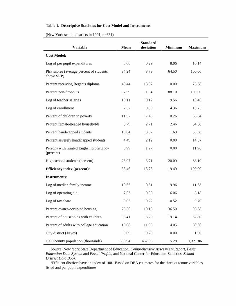
Table 1. Descriptive Statistics for Cost Model and Instruments

(New York school districts in 1991, n=631)

Variable Mean deviation Minimum MaximumStandard

Cost Model:

Log of per pupil expenditures 8.66 0.29 8.06 10.14

PEP scores (average percent of students 94.24 3.79 64.50 100.00above SRP)

Percent receiving Regents diploma 40.44 13.07 0.00 75.38

Percent non-dropouts 97.59 1.84 88.10 100.00

Log of teacher salaries 10.11 0.12 9.56 10.46

Log of enrollment 7.37 0.89 4.36 10.75

Percent of children in poverty 11.57 7.45 0.26 38.04

Percent female-headed households 8.79 2.71 2.46 34.68

Percent handicapped students 10.64 3.37 1.63 30.68

Percent severely handicapped students 4.49 2.12 0.00 14.57

Persons with limited English proficiency 0.99 1.27 0.00 11.96(percent)

High school students (percent) 28.97 3.71 20.09 63.10

Efficiency index (percent)a 66.46 15.76 19.49 100.00

Instruments:

Log of median family income 10.55 0.31 9.96 11.63

Log of operating aid 7.53 0.50 6.06 8.18

Log of tax share 0.05 0.22 -0.52 0.70

Percent owner-occupied housing 75.36 10.16 36.50 95.38

Percent of households with children 33.41 5.29 19.14 52.80

Percent of adults with college education 19.08 11.05 4.05 69.66

City district (1=yes) 0.09 0.29 0.00 1.00

1990 county population (thousands) 388.94 457.03 5.28 1,321.86

Source: New York State Department of Education, Comprehensive Assessment Report, BasicEducation Data System and Fiscal Profile, and National Center for Education Statistics, SchoolDistrict Data Book. Efficient districts have an index of 100. Based on DEA estimates for the three outcome variablesa

listed and per pupil expenditures.

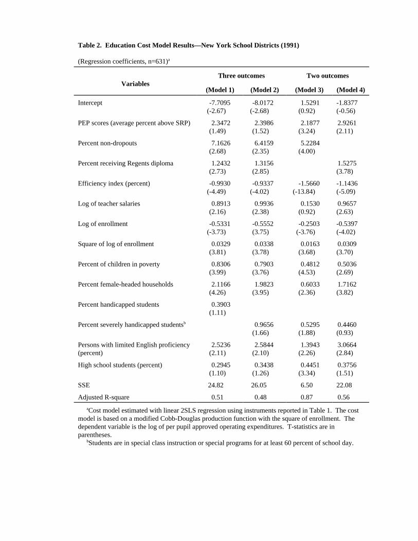
Table 2. Education Cost Model Results—New York School Districts (1991)

(Regression coefficients, n=631)a

VariablesThree outcomes Two outcomes

(Model 1) (Model 2) (Model 3) (Model 4)

Intercept -7.7095 -8.0172 1.5291 -1.8377(-2.67) (-2.68) (0.92) (-0.56)

PEP scores (average percent above SRP) 2.3472 2.3986 2.1877 2.9261(1.49) (1.52) (3.24) (2.11)

Percent non-dropouts 7.1626 6.4159 5.2284(2.68) (2.35) (4.00)

Percent receiving Regents diploma 1.2432 1.3156 1.5275(2.73) (2.85) (3.78)

Efficiency index (percent) -0.9930 -0.9337 -1.5660 -1.1436(-4.49) (-4.02) (-13.84) (-5.09)

Log of teacher salaries 0.8913 0.9936 0.1530 0.9657(2.16) (2.38) (0.92) (2.63)

Log of enrollment -0.5331 -0.5552 -0.2503 -0.5397(-3.73) (3.75) (-3.76) (-4.02)

Square of log of enrollment 0.0329 0.0338 0.0163 0.0309(3.81) (3.78) (3.68) (3.70)

Percent of children in poverty 0.8306 0.7903 0.4812 0.5036(3.99) (3.76) (4.53) (2.69)

Percent female-headed households 2.1166 1.9823 0.6033 1.7162(4.26) (3.95) (2.36) (3.82)

Percent handicapped students 0.3903(1.11)

Percent severely handicapped students 0.9656 0.5295 0.4460b

(1.66) (1.88) (0.93)

Persons with limited English proficiency 2.5236 2.5844 1.3943 3.0664(percent) (2.11) (2.10) (2.26) (2.84)

High school students (percent) 0.2945 0.3438 0.4451 0.3756(1.10) (1.26) (3.34) (1.51)

SSE 24.82 26.05 6.50 22.08

Adjusted R-square 0.51 0.48 0.87 0.56

Cost model estimated with linear 2SLS regression using instruments reported in Table 1. The costa

model is based on a modified Cobb-Douglas production function with the square of enrollment. Thedependent variable is the log of per pupil approved operating expenditures. T-statistics are inparentheses. Students are in special class instruction or special programs for at least 60 percent of school day.b

Table 3. Correlations between Education Cost Indices for New York State School Districts in 1991a

(n=631)

Socio-economic characteristics index) pupils cost index

Direct cost indices Indirect cost Cost indexindex based on

(No efficiency weighted Teacher salaryEndogenous No Exogenousefficiency efficiency efficiency

index

Standard deviation 16.93 26.11 10.85 15.33 8.88 12.75

Maximum 239.62 356.11 191.84 253.94 264.00 143.55

75th percentile 105.26 109.53 103.21 105.74 102.94 111.61

25th percentile 89.56 83.89 93.77 90.50 96.96 89.81

Minimum 77.50 70.70 83.83 77.05 44.68 68.37

Correlations:

Direct Cost Indices:

Endogenous efficiency index 1.00

No efficiency index 0.94 1.00

Exogenous efficiency index 0.84 0.74 1.00

Indirect cost index (no efficiency 0.63 0.55 0.39 1.00index)

Cost index based on weighted 0.14 0.15 0.13 0.08 1.00pupils

Teacher salary cost index 0.47 0.57 0.32 -0.08 0.06 1.00

Index for first three columns is based on 3-factor cost model (model 2 in Table 2) with the state average equal to 100. Index for fourth column isa

a reduced form model where the demand instruments—income, taxshare, and households with children—are substituted into the cost model foroutcome measures. The index in the fifth column is based on a ratio of weighted pupils over total enrollment; extra weight is given to secondary,handicapped and special needs pupils. The index in the last column is based on the relationship between teacher salaries and family and studentcharacteristics.

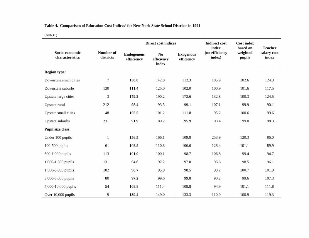
Table 4. Comparison of Education Cost Indices for New York State School Districts in 1991a

(n=631)

Socio-economic Number of (no efficiency weighted salary costcharacteristics districts index) pupils index

Direct cost indices Indirect cost Cost indexindex based on Teacher

Endogenous No Exogenouseffiiciency efficiency efficiency

index

Region type:

Downstate small cities 7 130.0 142.0 112.3 105.9 102.6 124.3

Downstate suburbs 130 111.4 125.0 102.0 100.9 101.6 117.5

Upstate large cities 3 179.2 190.2 172.6 132.8 100.3 124.5

Upstate rural 212 98.4 93.5 99.1 107.1 99.9 90.1

Upstate small cities 48 105.5 101.2 111.8 95.2 100.6 99.6

Upstate suburbs 231 91.9 89.2 95.9 93.4 99.0 98.3

Pupil size class:

Under 100 pupils 1 156.5 166.1 109.8 253.9 120.3 86.0

100-500 pupils 61 108.8 110.8 100.6 128.4 101.1 89.9

500-1,000 pupils 113 101.0 100.1 98.7 106.8 99.4 94.7

1,000-1,500 pupils 131 94.6 92.2 97.0 96.6 98.5 96.1

1,500-3,000 pupils 182 96.7 95.9 98.5 93.2 100.7 101.9

3,000-5,000 pupils 80 97.2 99.6 99.8 90.2 99.6 107.3

5,000-10,000 pupils 54 108.8 111.4 108.8 94.9 101.1 111.8

Over 10,000 pupils 9 139.4 149.0 133.3 110.9 100.9 119.3

Table 4. Continued

Socio-economic Number of (no efficiency weighted salary costcharacteristics districts index) pupils index

Direct cost indices Indirect cost Cost indexindex based on Teacher

Endogenous No Exogenouseffiiciency efficiency efficiency

index

Income class (percentile):

Under 10th 62 106.3 118.5 97.7 100.8 100.5 115.5

10th to 25th 95 99.8 105.4 97.3 100.8 100.2 109.4

25th to 50th 157 98.5 98.7 100.2 103.2 99.4 101.5

50th to 75th 159 98.7 95.7 100.8 111.4 99.5 95.0

75th to 90th 94 99.0 94.1 101.3 76.8 100.6 92.1

Over 90th 64 102.6 96.6 101.9 74.8 101.0 91.2

Property values (percentile):

Under 10th 63 109.7 122.9 98.7 111.7 100.1 109.1

10th to 25th 94 105.2 112.0 99.1 100.4 100.1 109.1

25th to 50th 158 99.8 100.5 100.0 97.6 99.5 101.9

50th to 75th 158 94.1 89.6 97.9 97.6 100.0 95.2

75th to 90th 95 96.7 91.0 100.7 98.7 99.7 94.5

Over 90th 63 103.0 97.5 106.8 101.7 101.3 92.9

Index for first three columns is based on 3-factor cost model (model 2 in Table 2) with the state average equal to 100. Index for fourth column isa

a reduced form model where the demand instruments—income, tax share and households with children—are substituted into the cost model foroutcome measures. The index in the fifth column is based on a ratio of weighted pupils over total enrollment; extra weight is given to secondary,handicapped and special needs pupils. The index in the last column is based on the relationship between teacher salaries and family and studentcharacteristics. Income is based on estimated per capita adjusted gross income in 1991 and property values are per capita market value for allproperty in 1990.

Table 5. Impact of Input and Environmental Variables on Education Costs, Districts with Highest and Lowest Costsa

Cost variables

10 percent of districts with highest costs 10 percent of districts with lowest costs

Index relative to state Percent of cost Index relative to Percent of costaverage difference due to state average difference due to(=100) variable (=100) variable

Total cost index 152.7 81.1

(Per pupil difference from average district) $3,046 -$1,091

Teacher salaries 111.2 30.67% 96.0 -20.03%

Log of enrollment 198.3 -13.20% 128.0 -18.85%

Percent of children in poverty 161.6 13.98% 49.4 -22.86%

Percent female-headed households 170.9 36.16% 75.3 -21.24%

Percent severely handicapped students 177.7 9.43% 54.3 -9.90%b

Limited English proficiency (percent) 407.6 22.47% 39.3 -7.77%

High school students (percent) 94.9 -1.38% 101.3 0.64%

Cost index based on 3-factor cost model (model 2 in Table 2). Indices for costs and environmental variables relative to state average are baseda

on average values for 10 percent of districts with the highest and lowest per pupil costs. The percentage cost difference due to cost variable i, sayPc , is based on three cost indices. Index A is the total cost index for the high-(or low-) cost districts. Index B is a cost index with all variables set ati

the state average. Index C is a cost index with cost variable i set at the average for the high-(or low-) cost districts and all other variables set at thestate average. Then, Pc = (C - B) / (A - C).i

Students are in special class instruction or special programs for at least 60 percent of school day.b

References

Baum, Donald. 1986. "A Simultaneous Equations Model of the Demand For and Production of Local

Public Services: The Case of Education," Public Finance Quarterly 14:157-78.

Bessent, A. and E.W. Bessent. 1980. "Determining the Comparative Efficiency of Schools through Data

Envelopment Analysis," Educational Administration Quarterly 16: 57-75.

Boardman, Anthony, Otto Davis, and Peggy Sanday. 1977. "A Simultaneous Equations Model of the

Education Process," Journal of Public Economics 7: 23-49.

Bradbury, Katharine, Helen Ladd, Mark Perrault, Andrew Reschovsky, and John Yinger.1984. "State

Aid to Offset Fiscal Disparities Across Communities," National Tax Journal 37 (June): 151-170.

Bradford, David, Robert Malt and Wallace Oates. 1969. "The Rising Cost of Local Public Services:

Some Evidence and Reflections," National Tax Journal 22 (June): 185-202.

Bridge, R. Gary, Charles Judd, and Peter Moock. 1979. The Determinants of Educational Outcomes:

The Impact of Families, Peers, Teachers and Schools. Cambridge, MA: Ballinger Publishing

Company.

Brown, Byron and Daniel Saks. 1975. "The Production and Distribution of Cognitive Skills in Schools,"

Journal of Political Economy 83: 571-593.

Callan, Scott and Rexford Santerre. 1990. "The Production Characteristics of Local Public Education: A

Multiple Product and Input Analysis," Southern Economic Journal 57 (October): 468-480.

Chambers, Jay. 1978. "Educational Cost Differentials and the Allocation of State Aid for Elementary and

Secondary Education," Journal of Human Resources 13: 459-481.

Chamber, Jay. 1980. "The Development of a Cost of Education Index: Some Empirical Estimates and

Policy Issues," Journal of Education Finance 5 (Winter): 262-281.

Charnes, A., W.W. Cooper and E. Rhodes. 1978. "Measuring the Efficiency of Decision Making Units,"

European Journal of Operational Research 2: 429-444.

Chizmar, John and Thomas Zak. 1983. "Modeling Multiple Outputs in Educational Production Functions,"

American Economic Review 73 (May): 18-22.

Cohn, Elchanan and Terry Geske. 1990. The Economic of Education. New York: Pergamon Press, 3rd

edition.

Cooper, Bruce. 1993. "Educational Choice: Competing Models and Meanings." In S. Jacobson and R.

Berne (eds.), Reforming Education: The Emerging Systemic Approach. Thousand Oaks, CA:

Corwin Press, Inc.

Downes, Thomas and Thomas Pogue. 1994. "Adjusting School Aid Formulas for the Higher Cost of

Educating Disadvantaged Students," National Tax Journal 47 (March): 89-110.

Duncombe, William. 1991. "Demand for Local Public Services Revisited: The Case of Fire Protection,"

Public Finance Quarterly 19: 412-436.

Duncombe, William and John Yinger. 1993. "An Analysis of Returns to Scale in Public Production, With

an Application to Fire Protection," Journal of Public Economics 52:49-72.

Duncombe, William, Jerry Miner and John Ruggiero. 1994. "Empirical Evaluation of Bureaucratic Models

of Inefficiency." Paper presented at the 1994 Annual Conference of the Southern Economic

Association, Orlando, FL, November 21.

Duncombe, William, Jerry Miner and John Ruggiero. 1995. "Potential Cost Savings from School District

Consolidation: A Case Study of New York," Economics of Education Review forthcoming.

Färe, Rolf and Knox Lovell. 1978. "Measuring the Technical Efficiency of Production," Journal of

Economic Theory 150-162.

Färe, Rolf, Shawna Grosskopf and William Weber. 1989. "Measuring School District Performance,"

Public Finance Quarterly 17: 409-428.

Farrell, M.J. 1957. "The Measurement of Productive Efficiency," Journal of the Royal Statistical

Society Series A, General, 120: 253-281.

Fenner, Richard. 1991. The Effect of Equity of New York State's System of Aid for Education. Ph.D.

dissertation. Syracuse University.

Ferguson, Ronald. 1991. "Paying for Public Education: New Evidence on How and Why Money Matters,"

Harvard Journal on Legislation 28: 465-498.

Fleeter, Howard. 1990. "District Characteristics and Education Costs: Implications of Compensating Wage

Differentials on State Aid in California." mimeo, Columbus, OH: Ohio State University.

Fuhrman, Susan, Richard Elmore and Diane Massell. 1993. "School Reform in the United States: Putting

It into Context." In S. Jacobson and R. Berne (eds.), Reforming Education: The Emerging

Systemic Approach. Thousand Oaks, CA: Corwin Press, Inc.

Gold, Steven, David Smith, Stephen Lawton, and Andrea C. Hyary. 1992. Public School Finance

Programs of the United States and Canada, 1990-91. Albany, New York: The Nelson A.

Rockefeller Institute of Government.

Grosskopf, Shawna and S. Yaisawarng. 1990. "Economies of Scope in the Provision of Local Public

Services," National Tax Journal 43: 61-74.

Gyimah-Brempong, Kwabena and Anthony Gyapong. 1991. "Characteristics of Education Production

Functions: An Application of Canonical Regression Analysis," Economics of Education Review

10: 7-17.

. 1992. "Elasticities of Factor Substitution in the Production of Education," Economics of Education

Review 11: 205-217.

Hanushek, Eric. 1979. "Conceptual and Empirical Issues in the Estimation of Educational Production

Functions," The Journal of Human Resources 14: 351-388.

. 1986. "The Economics of Schooling: Production and Efficiency in Public Schools," Journal of

Economic Literature 24: 1141-1177.

. 1994. Making Schools Work: Improving Performance and Controlling Costs. Washington,

D.C.: The Brookings Institution.

Inman, Robert. 1979. "The Fiscal Performance of Local Governments: An Interpretative Review." In P.

Mieszkowski and M. Straszheim (eds.), Current Issues in Urban Economics. Baltimore, MD:

The Johns Hopkins University Press, pp. 270-321.

Jimenez, Emmanuel. 1986. "The Structure of Educational Costs: Multiproduct Cost Functions for Primary

and Secondary Schools in Latin America," Economics of Education Review 5: 25-39.

Kumar, Ramesh. 1983. "Economies of Scale in School Operation: Evidence from Canada," Applied

Economics. 15: 323-340.

Ladd, Helen and John Yinger. 1991. America's Ailing Cities: Fiscal Health and the Design of Urban

Policy. Baltimore, MD: The Johns Hopkins University Press.

. 1994. "The Case for Equalizing Aid," National Tax Journal 47 (March): 211-224.

Miner, Jerry. 1991. "A Decade of New York State Aid to Local Schools," Metropolitan Studies Program

Occasional Paper No. 141, Center for Policy Research, The Maxwell School. Syracuse, NY:

Syracuse University.

Monk, David. 1990. Educational Finance: An Economic Approach. New York: McGraw-Hill

Publishing Company.

Monk, David and Billy Walker. 1991. "The Texas Cost of Education Index: A Broadened Approach,"

Journal of Education Finance 17 (Fall): 172-192.

Niskanen, W.A. 1971. Bureaucracy and Representative Government. Chicago: Aldine-Atherton.

. 1975. "Bureaucrats and Politicians," The Journal of Law and Economics 18: 617-643.

Odden, Allan and Lawrence Picus. 1992. School Finance: A Policy Perspective. New York: McGraw-

Hill, Inc.

Ratcliffe, Kari, Bruce Riddle, and John Yinger. 1990. "The Fiscal Condition of School Districts in

Nebraska: Is Small Beautiful?" Economics of Education Review 9: 81-99.

Reschovsky, Andrew. 1994. "Fiscal Equalization and School Finance," National Tax Journal 47

(March): 211-224.

Rubinfeld, Daniel. 1985. "The Economics of the Local Public Sector." In A. Auerback and M. Feldstein

(eds.), Handbook of Public Economics, Vol. 2. New York: Elsevier Science Publishers, pp.

571-645.

Ruggiero, John. 1994. "Are Costs Minimized in the Public Sector? A Nonparametric Analysis of the

Provision of Educational Services," Metropolitan Studies Program Occasional Paper No. 165,

Center for Policy Research, The Maxwell School. Syracuse, NY: Syracuse University.

. 1995a. "On the Measurement of Technical Efficiency in the Public Sector," European Journal of

Operational Research, forthcoming.

. 1995b. "Measuring Technical Inefficiency in the Public Sector: An Analysis of Educational

Production," Review of Economics and Statistics, forthcoming.

Seiford, L. and R. Thrall. 1990. "Recent Developments in DEA: The Mathematical Programming

Approach to Frontier Analysis," Journal of Econometrics 46: 7-38.

Serrano v. Priest, 1971. 487 P.2d 1241.

Schwab, Robert and Ernest Zampelli. 1987. "Disentangling the Demand Function from the Production

Function for Local Public Services: The Case of Public Safety." Journal of Public Economics 33:

245-260.

Summers, Anita and Barbara Wolfe. 1977. "Do Schools Make a Difference?" American Economic

Review 67 (September): 639-652.

Wendling, Wayne. 1981. "The Cost of Education Index: Measurement of Price Differences of Education

Personnel Among New York State School Districts," Journal of Education Finance 6 (Spring):

485-504.

Wyckoff, Paul G. 1988. "A Bureaucratic Theory of Flypaper Effects," Journal of Urban Economics 23:

115-129.

. 1990. "The Simple Analytics of Slack-Maximizing Bureaucracy," Public Choice 67:35-67.