Alt-Az Light Bucket Astronomy - Gravic, Inc

Chapter 2

The Alt-Az Initiative: Telescope, Mirror, & Instrument Devlopments. 2010. Genet, Johnson, & Wallen, eds.

Alt-Az Light Bucket AstronomyRussell Genet, California Polytechnic State University

Bruce Holenstein, Gravic Inc.

Introduction to Light Bucket AstronomyLight bucket alt-az telescopes are low optical quality light concentra-tors used in those areas of astronomical research where numerous low-cost photons are required but not an image per se. There is no more authoritative definition of astronomical terms than the Cambridge Dic-tionary of Astronomy (Mitton 2001):

light bucket A colloquial expression for a flux collector.flux collector A telescope designed solely to collect radiation in order to measure its intensity or to carry out spectral analy-sis. No attempt is made to form an image, so a flux collector can have a more crudely figured reflective surface than a con-ventional telescope.

We have generously extended light bucket status to “imaging” alt-az telescopes, but only if the images are decidedly fuzzy, the fields of view are somewhat narrow, and the “images” are just used for si-multaneous photometric measurements of the intensities of variable, comparison, and check objects.

Light bucket telescopes are, as we hereby further define them, low in cost, lightweight, and often pack easily for transport in small vehicles. Their instruments are also low cost, and the operations and mainte-nance of both the telescopes and their instruments can be performed by low cost non-specialized staff or no-cost volunteers.

Perhaps somewhat arbitrarily, we define an individual light bucket telescope as having an aperture between 1 and 3 meters. Light bucket telescopes can be divided into two major classes de-pending on their optical performance: (1) true on-axis light bucket flux collectors with many waves of aberration and (2) “fuzzy area” quasi light bucket telescopes with narrow fields of view and only a few waves of aberration. High optical quality telescopes are, of course, not light bucket telescopes.

58 Chapter 2 Russell Genet and Bruce Holenstein

Light bucket astronomy is advantageous in those situations where, compared to noise from the sky background, the noise from one or more other sources is dominant or, putting it the other way around, where the sky background is a small or nearly negligible source of noise. This situation can occur when (1) the object being observed is very bright, (2) the integration times are very short and hence photon arrival noise becomes important, (3) scintillation noise becomes a dominant noise source, (4) the bandwidth is very narrow or the light is spread out as in spectroscopy, resulting in significant photon arrival noise, or (5) noise from the detector is dominant (as it can be in the near infrared).

Some types of light bucket astronomy could benefit from an array of ultra low cost light bucket telescopes. Some interesting attributes of light bucket arrays include:

1. Reliability: The array elements operate separately and may provide immediate and independent confirmation of rare, transient events.

2. Availability: If a single scope in an array is removed from service due to a mechanical fault or mirror-aluminizing, the rest of the array will keep operating at virtually no reduction in performance. In other words, the array fails gracefully rather than all at once.

3. Independence: If the array is spread out over a substantial geo-graphic area, clouds and other environmental factors will not disable (e.g. “cloud out”) the entire array. Continuous coverage of the night sky might be possible if multiple continents are included in the geographic extent.

4. Transportability: If individual light bucket array telescopes are moveable, the array may be repositioned to avoid a storm or seek out an ideal location for an asteroid occultation event. GPS or laser ranging may be used to re-collimate the array.

5. Expandability: As funds and time allow, additional array elements may be added to increase the scientific reach of the telescope. One may also replace or upgrade (e.g. resurface) the mirrors in order to work on deeper sky objects.

Signal-to-Noise RatioThe major factors that influence the overall signal-to-noise ratio (SNR) of program object measurements include the amount of both program object and background sky flux collected, scintillation, air mass, filter bandpass, and detector and readout noises. In order to understand some of the tradeoffs visually, the figure below displays figures of merit for the relative SNR for light bucket telescopes of 1.0 and 1.5 me-ter apertures relative to a 40 cm (16 inch) diffraction-limited Schmidt-

59Alt-Az Light Bucket Astronomy

Cassegrain telescope as a function of program object brightness. A 40 cm SCT was chosen because we thought that its cost might be roughly equivalent to that of a 1 to 1.5 m light bucket telescope. Equation 20 of Holenstein et. al. (2010) was used for the calculations.

Figure 1: Relative signal-to-noise ratio of a light bucket telescope as compared to a smaller aperture but higher optical quality telescope.

Shown in the Figure 1 graph, the SNR of both 1.0 m f/3 and 1.5 m f/2 light bucket telescopes was divided by the SNR of a 40 cm f/10 diffraction-limited Schmidt-Cassegrain (SCT) telescope as a function of the luminosity of the program object. The background sky is 21 magnitudes/arcsec2. The 40 cm telescope uses a 20 μm (1”) focal plane diaphragm. The illustrated cases are for 100 μm (7”) and 400 μm (28”) diaphragms for each of the 1.0 and 1.5 meter telescopes. A relative SNR of 1.0 means that the two telescopes have the same photometric perfor-mance. Scintillation is calculated according to Young (1967) at a 1000 meter elevation with an air-mass of 1.5. Amplifier and detector noise is modeled by an Optec SSP-5a with a Hamamatsu R6358 multi-alkali photomultiplier tube and a Johnson B filter.

For very bright program objects, scintillation takes over and limits the relative performance to a value that approaches the expected value based of the relative sizes of the telescope apertures. The relative SNR for mid-brightness objects peaks at a value which approaches the ra-tio of the example telescope apertures. For faint program objects, the


traditional telescope in some cases outperforms the light bucket ones, depending on the size of the focal plane diaphragms. However, note that no allowance is made in the figure for program objects for which the diaphragm is unable to isolate the detector from field stars. Errors caused by program object tracking problems have been analyzed (Ho-lenstein et. al. 2010).

The SNR crossover point of 1.0 depends on the relative size of the focal plane diaphragms and the apertures of the light bucket telescopes. For mid-brightness objects, the light bucket telescopes excel. For ex-ample, a relative SNR of 3 means that a 3 hour run with the SCT scope may be accomplished with the light bucket in one-third squared, or one-ninth, the time, i.e. 20 minutes. Another way of looking at the situation in this example is that the productivity of the light bucket is nine times higher than the SCT. Nine times the number of program objects may be observed at the same SNR level as the SCT is able to obtain per unit of observing session. But, it is not just a question of the economics of observing time. In many scenarios the more important factor is the SNR achievable in a set short integration time for fast changing objects. For example, if one wants to observe a flare star with 10 ms time resolution, a factor of three improvement in the SNR achieved may make all the difference in the world in the interpretation of the observation results.

The Hipparcos catalog contains 118,000 stars brighter than visual apparent magnitude 7.3. The Tyco-2 catalog contains 2.5 million stars to about V ~ 11th magnitude. For every magnitude fainter than that, one adds in about 300% more stars. As a result, there is rarely a shortage of interesting program objects at accessible apparent magnitudes com-pared to the background brightness.

The graph above is easy to adjust for observing sites where the background sky is brighter than 21 magnitudes/arcsec2. For example, in a suburban city location, the sky brightness might be 17 magnitudes/arcsec2. Since this setting is four magnitudes brighter, just subtract 4 from each value of the ordinate (i.e. the X-axis). So, 21 becomes 17 mag-nitudes/arcsec2, 20 becomes 16 magnitudes/arcsec2, and so on. Note that this adjustment is actually only approximate for the fainter objects due to the scaling relationship of the detector/amplifier noise.

Light Bucket Research AreasAt an Alt-Az Initiative workshop held in conjunction with the Ameri-can Astronomical Society summer meeting in Pasadena in 2009, Arne Henden, the Executive Director of the American Association of Vari-able Star Observers, gave a talk entitled “1.5 Meter Light Bucket As-tronomy.” Arne outlined the key research areas where light buckets


excel. These include high speed photometry, near IR photometry, time series spectroscopy, and fast cadence/high precision photometry.

One of the most interesting areas for high speed photometry is the interference (fringe) light curves produced when the Moon (or another solar system body) occults stars and data is obtained at milli-second intervals. Analysis of these fringe patterns can yield stellar diameters for nearby stars and discover new close binary stars with separations of just a few milli-arc seconds (Nather et al. 1970, Beavers et al. 1980, Ridgeway et al. 1980, Feckel et al. 1980, Schmidtke et al. 1984, Peterson et al. 1989, Richichi 1984, van Belle et al. 2002, Richichi et al. 2008, 2009). Obtaining a decent number of photons for each milli-second interval requires a large photon gathering area, although only on-axis light concentration is required if a high speed photodiode or photomultiplier is used as the detector. Brian Warner (1988) wrote the classic book on high speed photometry, while two more modern books are those edited by the trio of Don Phelan, Oliver Ryan, and Andrew Shearer (both 2008).

Figure 2: The diameters and duplicity of nearby stars can be determined through analysis of high speed photometry of lunar occultations.

Shown in Figure 2 are the theoretical diffraction pattern light curves (320-720 nm bandpass) for the lunar occultation of three stars: small with a 0.1 milli-arc second (mas) diameter, medium with 2 mas, and large with 10 mas (each with a small companion having just 10% of the luminosity of the primary). Limb darkening is set to zero and


the location of the companions form the primary trails by 10, 15, and 20 mas respectively. The diffraction pattern sweeps over the ground in milliseconds, depending on the orientation of the moon’s limb.

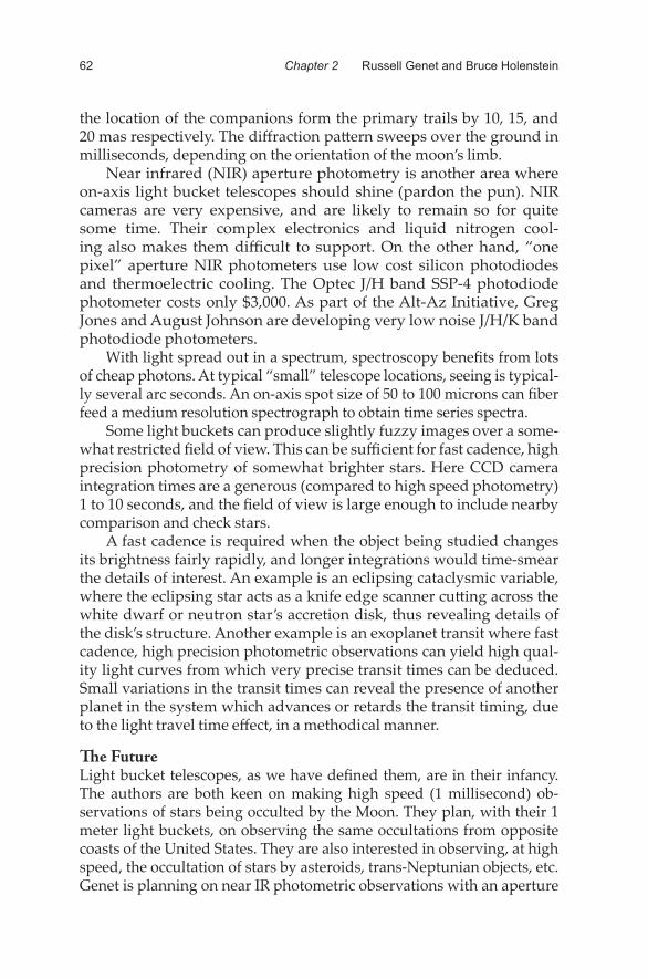
Near infrared (NIR) aperture photometry is another area where on-axis light bucket telescopes should shine (pardon the pun). NIR cameras are very expensive, and are likely to remain so for quite some time. Their complex electronics and liquid nitrogen cool-ing also makes them difficult to support. On the other hand, “one pixel” aperture NIR photometers use low cost silicon photodiodes and thermoelectric cooling. The Optec J/H band SSP-4 photodiode photometer costs only $3,000. As part of the Alt-Az Initiative, Greg Jones and August Johnson are developing very low noise J/H/K band photodiode photometers.

With light spread out in a spectrum, spectroscopy benefits from lots of cheap photons. At typical “small” telescope locations, seeing is typical-ly several arc seconds. An on-axis spot size of 50 to 100 microns can fiber feed a medium resolution spectrograph to obtain time series spectra.

Some light buckets can produce slightly fuzzy images over a some-what restricted field of view. This can be sufficient for fast cadence, high precision photometry of somewhat brighter stars. Here CCD camera integration times are a generous (compared to high speed photometry) 1 to 10 seconds, and the field of view is large enough to include nearby comparison and check stars.

A fast cadence is required when the object being studied changes its brightness fairly rapidly, and longer integrations would time-smear the details of interest. An example is an eclipsing cataclysmic variable, where the eclipsing star acts as a knife edge scanner cutting across the white dwarf or neutron star’s accretion disk, thus revealing details of the disk’s structure. Another example is an exoplanet transit where fast cadence, high precision photometric observations can yield high qual-ity light curves from which very precise transit times can be deduced. Small variations in the transit times can reveal the presence of another planet in the system which advances or retards the transit timing, due to the light travel time effect, in a methodical manner.

The FutureLight bucket telescopes, as we have defined them, are in their infancy. The authors are both keen on making high speed (1 millisecond) ob-servations of stars being occulted by the Moon. They plan, with their 1 meter light buckets, on observing the same occultations from opposite coasts of the United States. They are also interested in observing, at high speed, the occultation of stars by asteroids, trans-Neptunian objects, etc. Genet is planning on near IR photometric observations with an aperture


photometer—the Optec SSP-4 and/or a photometer being developed by Greg Jones—as well as fast cadence, high precision “fuzzy” CCD pho-tometry of eclipses of cataclysmic variables and exoplanet transits.

Larger aperture light bucket telescopes are on the drawing boards. How rapidly this field progresses will critically depend, of course, on the development of unusually lightweight, low cost, low optical quality mirrors. We expect that, depending on the specific mirror technology, an economically optimal individual mirror size may emerge—perhaps 1 meter for meniscus plate glass or foam glass mirrors. Four 1 meter mirrors could be combined to form a 2 meter equivalent aperture light bucket telescope that, being less than 8 feet wide, could be towed down the road in a lowboy trailer.

Seven 1 meter mirrors, left round or water jetted into hexes, would produce, respectively, 2.6 meter equivalent aperture versions of the Gi-ant Magellan Telescope (GMT) or the Thirty Meter Telescope (TMT). Perhaps they could be dubbed the Mini Magellan Telescope (MMT) or Three Meter Mini (TMM). Such a light bucket telescope might be light enough to transport down the road, pulled by a pickup or SUV. Their core azimuth bases could remain intact as roll on/off assemblies, although on-site assembly of the rest of the telescopes would probably be required. If individual mirrors only weighed 50 lbs, then assembly by two persons without any mechanical assistance should be possible.

Arrays of Light Bucket TelescopesWe cannot resist mentioning the ultimate light bucket astronomy dream—an array of six or seven lightweight, low cost, sizeable (2 to 4 meter), on-axis light buckets that could, as an array, image the surface of nearby stars via intensity interferometry. Stellar intensity interfer-ometry, based on a sub-nanosecond quantum-mechanical effect, was pioneered by Hanbury Brown many decades ago with a two-telescope system on a 188 meter circular track (Hanbury Brown 1956, 1974). Movement of the telescopes along this track kept the spacing between them constant and their baseline orthogonal to the incoming starlight. Changing the spacing between the telescopes provided the crucial in-terferometric information. Hanbury Brown used an analog correlator to compare the high speed signals from photomultiplier tubes at prime focus on the two telescopes.

Picture six or seven of the 2 to 4 meter light bucket telescopes described above, spaced out as an intensity interferometer array in somebody’s generously proportioned back yard. Like the VLA radio telescope, the individual telescopes could be positioned to optimize specific observations. During periods of inclement weather, they could all be wheeled into a low cost storage barn.


Figure 3: R. Hanbury Brown’s stellar intensity interferometer located in Narrabri, Australia. Galileo attempted to measure the diameter of Vega, but it took the Narrabri interferometer to finally make the measurement (about two milli-arc seconds). During periods of poor weather, the telescopes were moved along the track into a storage shed.

In the decades since Hanbury Brown’s pioneering work, not only has the quantum efficiency and speed of detectors greatly improved, but very high-speed digital correlators are now possible. A revival of stellar intensity interferometry by use of Cherenkov telescope arrays has been contemplated (LeBohec and Holder 2006, LeBohec et. al. 2008) and a workshop on modern stellar intensity interferometry was held in Utah (LeBohec 2009).

Hanbury Brown derived the following formula for the SNR of his device:

where A is the telescope area; α is the photomultiplier quantum effi-ciency; n is the number of photons incident on the telescope per unit area, per unit time, and optical bandwidth; γ is the degree of coherence of the flux; Δf is the bandpass of the electronics; and T is the observ-ing period. When multiple channels and path lengths are measured simultaneously, the following formula describes the overall SNR of the system:


where NArray is the number of elements in the array, and NChannels is the number of simultaneous channels measured, and the noise is modeled as adding in quadrature.

The following is an estimate of the potential relative performance of a modern stellar intensity interferometer with a pair of 2 meter light bucket mirrors compared to Hanbury Brown’s 6.5 meter aper-ture device. First, Hanbury Brown used an extremely narrow optical bandwidth for his observations, specifically a single interference filter, which was typically just 4 nm wide. There is no reason that the modern device could not use a low to medium resolution spectrograph and a high speed, higher quantum efficiency detector array containing one hundred or more high-speed (sub-nanosecond resolution multialkali PMTs or avalanche diode) detectors. Additionally, Hanbury Brown’s analog electronics had a bandpass of about 60MHz. Modern electronics and DSP correlators can operate at least a factor of 100 times faster.

Using Equations 1 and 2, the overall SNR improvement due to these factors scales directly as the mirror collection area and relative quantum efficiency times the square root of the product of the relative bandwidth and number of channels, all other terms being held approximately constant. In this example case with two 2 meter telescopes only having 1/10th the area but with 100 channel detector/correlators operating at 100 times the speed with about three times the quantum efficiency, we have: (0.1) x (3) x (100 x 100)1/2 equals a factor of thirty times better per-formance for the modern instrument. So, the much smaller (2 instead of 6.5 meters) modern intensity interferometer might operate three or more magnitudes fainter than Hanbury Brown’s interferometer.

While Hanbury Brown was able to determine the diameters of 32 of the nearest stars, a modern array of a half-dozen or more light bucket telescopes with its many path length permutations could provide ac-tual images of large nearby stars, complete with starspots and strange shapes as, for instance, red giants shed their mass. Using Equation 2, a seven-element array has up to 7x6/2 = 21 unique baselines (some may be degenerate depending on telescope placement, program object location, and other geometrical factors) which corresponds up to a 4.6 times improvement in the overall SNR with all other factors held constant. This corresponds to another factor of 1.5 magnitudes over the three plus magnitudes already calculated. Clearly, stellar intensity interferometry with light bucket telescopes deserves some close atten-tion for further feasibility analysis. Also, note that the modern equip-ment might also be used to look for natural lasers, for example in hot systems such as Eta Carinae, through photon-correlation spectroscopy (Dravins and Germanà 2008).


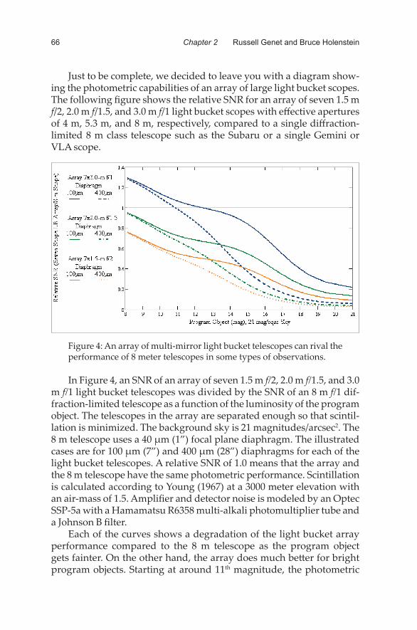
Just to be complete, we decided to leave you with a diagram show-ing the photometric capabilities of an array of large light bucket scopes. The following figure shows the relative SNR for an array of seven 1.5 m f/2, 2.0 m f/1.5, and 3.0 m f/1 light bucket scopes with effective apertures of 4 m, 5.3 m, and 8 m, respectively, compared to a single diffraction-limited 8 m class telescope such as the Subaru or a single Gemini or VLA scope.

Figure 4: An array of multi-mirror light bucket telescopes can rival the performance of 8 meter telescopes in some types of observations.

In Figure 4, an SNR of an array of seven 1.5 m f/2, 2.0 m f/1.5, and 3.0 m f/1 light bucket telescopes was divided by the SNR of an 8 m f/1 dif-fraction-limited telescope as a function of the luminosity of the program object. The telescopes in the array are separated enough so that scintil-lation is minimized. The background sky is 21 magnitudes/arcsec2. The 8 m telescope uses a 40 μm (1”) focal plane diaphragm. The illustrated cases are for 100 μm (7”) and 400 μm (28”) diaphragms for each of the light bucket telescopes. A relative SNR of 1.0 means that the array and the 8 m telescope have the same photometric performance. Scintillation is calculated according to Young (1967) at a 3000 meter elevation with an air-mass of 1.5. Amplifier and detector noise is modeled by an Optec SSP-5a with a Hamamatsu R6358 multi-alkali photomultiplier tube and a Johnson B filter.

Each of the curves shows a degradation of the light bucket array performance compared to the 8 m telescope as the program object gets fainter. On the other hand, the array does much better for bright program objects. Starting at around 11th magnitude, the photometric


performance of the 3 m light bucket array exceeds that of the 8 m telescope. The smaller 1.5 m array even has 60% or more of the perfor-mance of the 8 m telescope starting around 10th magnitude.

ConclusionsIn this paper we defined light bucket telescopes as flux collectors which are low in cost, lightweight, and often pack easily for transport in small vehicles. Their instruments are also low cost, and the operations and maintenance of both the telescopes and their instruments can be performed by low cost non-specialized staff or no-cost volunteers. We further, somewhat arbitrarily, defined an individual light bucket tele-scope as having an aperture between 1 and 3 meters and comprising two major classes depending on their optical performance: (1) true on-axis light bucket flux collectors with many waves of aberration and (2) “fuzzy area” quasi-light bucket telescopes with narrow fields of view and only a few waves of aberration.

Some important conclusions about light bucket telescopes we pointed out are as follows:

• Light bucket astronomy is advantageous in those situations where, compared to noise from the sky background, the noise from one or more other sources is dominant or, putting it the other way around, where the sky background is a small or nearly negligible source of noise. When this condition is met, light bucket telescopes may produce measures with a superior SNR compared with a smaller traditional diffraction-limited telescope costing about the same amount. Alternately, the light bucket telescope may produce measures at a faster cadence at the same SNR level.

• Areas suitable for light bucket research include high speed photometry, near IR photometry, time series spectroscopy, and fast cadence/high precision photometry, lunar and solar system occultations, and polarimetry.

• Arrays of light bucket telescopes can extend greatly the ability to observe objects of interest at a desirable SNR. High-speed detec-tors and electronics, GPS and the use of lasers for collimation, may in some situations allow light bucket telescope arrays to challenge the scientific performance of giant professional tele-scopes at orders of magnitude less cost. Some projects possible with light bucket telescope arrays in the near future are not even attainable with the other instruments due to performance, costs, or competition for telescope time. An interesting example of this class of project is a revival of stellar intensity interferometry.


AcknowledgementsThe authors wish to thank and acknowledge the following people who have inspired this work, including Arne Henden, Robert Koch, Stephan LeBohec, Dave Rowe, Charlie Warren, various members of the Alt-Az Initiative, and of course, the late R. Hanbury Brown. Additionally, we must express our appreciation for the patience of co-editors and pro-duction staff members Vera Wallen, Jo Johnson, and Cheryl Genet for putting up with our numerous changes and re-writes.

ReferencesBeavers, W. I., Eitter, J. J., Dunham, D. W., & Stein, W. L. 1980. Lunar occulta-

tion angular diameter measurements. Astronomical Journal, 85, 1505-1508.Dravins, D. and Germanà, C. 2008. Photon correlation spectroscopy for observ-

ing natural lasers. In High Time Resolution Astrophysics, eds. D. Phelan, O. Ryan, and A. Shearer. New York: Springer.

Fekel, F.C., Montemayor, T. J., Barnes III, T. G., & Moffett, T. J. 1980. Pho-toelectric observations of lunar occultations. Astronomical Journal, 85, 490-494.

Hanbury Brown, R. 1956. A test of a new type of stellar interferometer on Sirius. Nature 178, 1046-1048.

Hanbury Brown, R. 1974. The Intensity Interferometer. London: Taylor & Francis Ltd.

Holenstein, B. D., Mitchell, R. J., and Koch, R. H. 2010. Figures of merit for light bucket mirrors. In The Alt-Az Initiative: Telescope, Mirror, and Instrument Developments, eds. R. Genet, J. Johnson, and V. Wallen. Santa Margarita, CA: Collins Foundation Press.

LeBohec, S. 2009. The Workshop on Stellar Intensity Interferometry: January 29 and 30 2009, University of Utah, http://www.physics.utah.edu/~lebohec/SIIWGWS/ (accessed March 2010)

LeBohec, S., Daniel, M., de Wit, W. J., Hinton, J. A., Jose, E., Holder, J. A., Smith, J., and White, R. J. 2008. Stellar intensity interferometry with air Cherenkov telescope arrays. In High Time Resolution Astrophysics, eds. D. Phelan, O. Ryan, and A. Shearer. New York: Springer.

LeBohec, S. and Holder, J. A. 2006. Optical intensity interferometry with atmospheric Cherenkov telescope arrays. Astrophysical Journal, 649, 399–405.

Mitton, J. 2001. Cambridge Dictionary of Astronomy. Cambridge, UK: Cam-bridge University Press.

Nather, R. E. & Evans, D. S. 1970. Photoelectric measurement of lunar oc-cultations. I. The process. Astronomical Journal, 75, 575-582.


Peterson, D. M., Baron, R., Dunham, E. W., Mink, D., Aldering, G., Klavetter, J., and Morgan, R. 1989. Lunar occultations of Praesepe II. Astrophysical Journal, 98, 2156-2158.

Phelan, D., Ryan, O., and Shearer, A. 2008. High Time Resolution Astrophys-ics. New York: Springer.

Phelan, D, Ryan, O., and Shearer, A. 2008. The universe at sub-second times-cales. AIP 2008 Conference Proceedings, 984.

Richichi, A. 1984. Model-independent retrieval of brightness profiles from lunar occultation lightcurves in the near infrared domain. Astronomy & Astrophysics, 226, 366-372.

Richichi, A., Barbieri, C., Fors, O., Mason, E., and Naletto, G. 2009. The beauty of speed. The Messenger, 135, pp. 32-36.

Richichi, A., Fors, O., and Mason, E. 2008. Milliarcsecond angular resolution of reddened stellar sources in the vicinity of the Galactic center. Astrono-my & Astrophysics, 489, 1441-1453.

Ridgway, S. T., Jacoby, G. H., Joyce, R. R., and Wells, D. C. 1980. Angular diameters by the occultation technique. III. Astronomical Journal, 85, 1496-1504.

Schmidtke, P. C. & Africano, J. L. 1984. KPNO lunar occultation summary I. Astronomical Journal, 89, 1371-1378.

van Belle, G. T., Thompson, R. R., and Creech-Eakman, M. J. 2002. Angular size measurements of Mira variable stars at 2.2 microns. II. Astronomical Journal, 124, 1706-1715.

Warner, B. 1988. High Speed Astronomical Photometry. New York: Cambridge University Press.

Young, A. T. 1967. Photometric error analysis: confirmation of Reiger’s theory of scintillation. Astrophysical Journal, 72, 747-753.

Alt-Az Light Bucket Astronomy - Gravic, Inc

Documents

Transcript of Alt-Az Light Bucket Astronomy - Gravic, Inc