1

Alpha and Beta of Buyout Deals: A Jump CAPM for Long-Term Illiquid Investments

Ulf Axelson*

Morten Sorensen**

Per Stromberg***

PRELIMINARY

COMMENTS WELCOME

November, 2014 * London School of Economics: U.Axelson@lse.ac.uk; ** Columbia Business School: ms3814@columbia.edu; *** Stockholm School of Economics: Per.Stromberg@sifr.org. We are grateful to Peter Cornelius and Robert de Veer for their support of this project. Mattia Landoni provided outstanding research assistance. We thank Michael Johannes, Neng Wang, and seminar participants at Columbia Business School for helpful discussions and suggestions. All remaining errors are our own.

  2

This paper estimates the risk and performance of buyout transactions. In a typical buyout

deal, a buyout fund acquires a company. The fund becomes the sole shareholder, and a

large fraction of the acquisition price is financed with debt. The fund then owns and

manages the company for an extended period of time, typically several years, until the

company is eventually sold in an exit, either into the public market, to a corporate

acquirer, or to another buyout fund (or liquidated). We evaluate the risk and risk-adjusted

performance that buyout funds generate on their equity investments in these deals. We

find an alpha of 8.3%-8.6% annually, and a beta of 2.2-2.4. These numbers represent the

total return earned on the levered equity investment in the buyout deals, gross-of-fees,

and the return is shared between the limited partners (“LP”), which provide the capital to

the fund, and the general partner (“GP”), which charges carried interest and management

fees for managing the fund.

Evaluating the risk and performance of buyout deals is important. When assessing

the role of buyout transactions in the economy, it would be a concern if these transactions

were financially underperforming the market. Moreover, the risk and performance are

important for LPs, such as pension funds, university endowment, and sovereign wealth

funds, which manage PE investments. Our analysis considers the return to the equity

invested in individual buyout deals, but LPs are obviously mostly concerned about the

aggregate risk and return of an entire fund, net of carried interest and management fees.

In order to evaluate fund-level performance, however, it is useful to start from the

individual deals and aggregate up to fund-level performance. Most existing studies have

evaluated buyout performance using data that aggregate fund-level net-of-fees cash flows,

  3

without attributing these cash flows to the individual deals. For example, Kaplan and

Schoar (2005) regress fund-level IRRs on S&P-500 and report a coefficient of 0.38-0.41.

Franzoni, Nowak, and Phalippou (2011) and Driesssen, Lin, and Phalippou (2011)

estimate other one-factor market models and report market betas of 0.9 and 1.3-1.5.

Jegadeesh, Kraussl, and Pollet (2010) take another approach and estimate alpha and betas

of publicly-traded private equity funds, and find betas of 0.7-1.0.

Betas around 1.0 are puzzling, though. A simple Modigliani-Miller (1958)

calculation suggests that the beta should be 2.2-2.7. To see this, note that Axelson,

Jenkinson, Stromberg, and Weisbach (2013) find an average D/E ratio around 3.0 in a

sample of buyout transactions (i.e., a typical buyout deal is financed with 75% debt and

25% equity). By definition, publicly-traded companies have an average levered beta (or

equity beta) of one, and with an average D/E ratio of 0.5, their unlevered beta (or asset

beta) is 0.66. After matching portfolio companies in buyout deals to their publicly-traded

comparable counterparts, Ljungqvist and Richardson (2003) find average betas for these

comparable companies of 1.04-1.13, suggesting that portfolio companies in buyout

transactions have average betas and hence also have unlevered betas of 0.66. With a D/E

ratio of 3.0, Modigliani-Miller then implies a levered equity beta of 2.7. A beta of 2.7

may be too high, however, because this calculation assumes risk-free debt. With a debt

beta of 0.1 (Kaplan and Stein, 1990), the equity beta becomes 2.2. This beta, however, is

still far above the betas of 0.7-1.5 from previous empirical studies. These studies suggest

that buyout funds can acquire regular companies with equity betas around 1.0 and then

increase their leverage six-fold, yet leave their systematic risk unchanged. This “beta

puzzle” challenges our understanding of the relationship between leverage and risk.

  4

There are three potential explanations for this puzzle: First, the betas found using

deal-level cash flows may be downward biased and underestimate the true value. Second,

the GP’s fees may reduce the beta. The Modigliani-Miller calculation applies to the

equity investment in the deal, gross of fees, whereas the fund-level cash flows used in

previous studies are reported net of fees. Third, Modigliani-Miller may not apply to the

portfolio companies of buyout funds. The process of acquiring these companies, taking

them private, and restructuring their governance may change their financial performance

and reduce their risk exposure relative to publicly-traded companies. Investigating these

explanations, we find some support for the first two explanations, but we find no support

for the third one.

To evaluate the risk and performance of buyout transactions, we face two

difficulties: First, deal-level performance data for buyout investments are highly

confidential and they have been difficult to access for academic researchers. We present a

new such dataset obtained from a large fund-of-funds, referred to as “The LP.” The LP

manages more than USD 50 billion of investments in buyout and venture capital funds,

and the dataset contains the LP’s internal deal-level cash-flow information for 2,075

buyout deals, managed by around 250 funds. Importantly, the LP compiles performance

data gross of the GPs’ “carried interest,” enabling us to compare the gross- and net-of-fee

risks, which helps resolve the second explanation for the “beta puzzle.” Second, the long-

term illiquid nature of buyout deals means that their performance is not well described by

standard asset pricing models, which are more designed for traded securities with

regularly quoted returns. Hence, we evaluate buyout performance using a range of

  5

models, and provide some extensions of these models to better capture the long-term

illiquid nature of buyouts.

Three related papers have estimated deal-level performance of venture capital

(“VC”) investments, which have structures that are similar to buyout deals, but for which

data with individual transaction have been more readily accessible. Gompers and Lerner

(1997) estimate the static capital asset pricing model (“CAPM”) using the deals of a

single VC firm (Warburg Pincus) from 1972 to 1977, and they find an alpha of 30.5%

with a beta of 1.08-1.44. Cochrane (2005) and Korteweg and Sorensen (2011) argue that

venture capital data suffer from a severe selection bias, because better-performing start-

ups are more frequently observed in the data and underperforming start-ups tend to

disappear without any observed exit or liquidation event, and they develop various

dynamic sample selection corrections. This sample selection problem is a smaller concern

for buyout deals, because buyout transactions involve mature companies and these

companies have well-defined and observed exit events, even when this exit is bankruptcy

or liquidation.

Finally, two studies have evaluated the performance of buyout investments using

fund-level data without directly estimating the risks of these investments.1 Ljungqvist

and Richardson (2003) analyze data from another large LP investing during 1981-1993

(in a total of 19 VC funds and 54 buyout funds), assuming that these deals have the same

risk as comparable publicly-traded companies. Kaplan and Schoar (2005) evaluate fund-

                                                                                                               1 Two recent surveys are Ang and Sorensen (2013) and Meyer, Cornelius, Diller, and Guennoc (2013).

  6

level buyout performance using data from Venture Economics, of which 746 funds were

fully or mostly liquidated at the time of the study, assuming a beta of one.

I. Data and Return Measures

Our data are provided by a large fund-of-funds, which we refer to as the LP. The LP is

one of the world’s largest investors in private equity, including both buyout and venture

capital funds. The LP has collected performance data for most of the individual deals

made by the funds in which it invested as an LP. Our performance data are current as of

February 2013, but we limit our sample to investments made up to 2008 to give these

deals time to mature. Before 2008, the LP has invested in around 250 buyout funds, and

we have performance information for 2,075 deals. Stromberg (2007) report that the total

PE industry, at the time, comprised around 8,000 deals. Today, the LPs overall private

equity allocation (including venture capital) exceeds USD 50 billion.

The LP classifies buyout funds as either: Large cap, US mid-market, EU mid-

market, or non-traditional markets (“NTM”) funds. Loosely defined, large cap funds are

funds with total committed capital exceeding USD 5 billion, although in the earlier part

of our sample, during the 1990s, this cut-off was lower. Mid-market funds typically have

fund sizes between USD 500 million and 5 billion. Funds classified as non-traditional

markets (“NTM”) include funds that focus on Advanced Asia (primarily Japan, and

Australia), Emerging Asia (primarily China and India), Latin America, and Eastern

Europe. Although not included in this study, The LP also invests in venture capital funds,

which invest in early and later-stage startups, including some growth-capital funds that

are managed by venture capital GPs.

  7

B. Cash Flow Data

The LP collects cash-flow information for most of the individual buyout deals

undertaken by the funds in which it has invested, including the timing and amounts of

these cash flows. Typically, for buyout investments, these cash flows consist of an initial

investment followed by an ultimate exit. The recorded cash flows are gross of the

“carried interest,” which is the performance fees charged by the PE firm that is the fund’s

general partner (“GP”). Moreover the cash flow data do not subtract management fees.

Due to this absence of fees, we can evaluate risk and return gross-of-fees, which are

comparable to the Modigliani-Miller calculation in the introduction. We then subtract the

fees and evaluate their effects on the risk and return. We have performance information

for 2,075 individual deals, and the timing of these deals is reported in Table I.

--- TABLE I ---

C. Return Measures

To distinguish different return measures, let the annualized arithmetic return be

denoted uppercase R. When a deal has only two associated cash flows, an initial

investment, I(t), and a subsequent exit, X(t’), then R is given as:

R = X( ′t )I(t)

⎛⎝⎜

⎞⎠⎟

1′t −t−1 . (1)

Without intermediate cash flows, R equals the internal rate of return (“IRR”), as

commonly defined. With intermediate cash flows, due to interim recapitalizations or

  8

equity injections, this return is not well defined and instead we define R as the IRR of the

deal’s cash flows. The total arithmetic return is R( ′t ,t) = (R +1) ′t −t −1 .  We use lowercase

r(t,t’) to denote log-returns. The total log-return is r( ′t ,t) = ln R(t, ′t )+1( ) , and the

annualized log-return is r = r(t, ′t )′t − t

.  

To illustrate, a $1 initial investment that turns into a $3 exit after 5 years will have

a total return of R(0,5) = 200%, an annualized return of R = 24.6%, a total log-return of

r(0,5) = 109.9%, and an annualized log-return of r = 22.0%. For smaller values, the log-

return is close to the arithmetic return. For larger values, these two returns are not directly

comparable. One inherent limitation of the log-return is that the calculation fails for

returns of -100%. In our data, 479 out of 2,075 buyout deals had returns of -100%. In

these cases, we set the log-return to -3, corresponding to a -95% arithmetic return. We

find that value of this cut-off has very little effect on our results, and we also report

estimates of a Tobin model that explicitly accounts for the left-truncation of the return

distribution.

Let RM(t,t’) denotes the total return on the public market over the corresponding

period, and similarly let RM, rM, and rM(t,t’) denote the annualized return, annualized log-

return, and total log-return on the public market. Risk-free returns are defined

analogously. All market returns and risk-free rates are calculated from market data

downloaded from Kenneth French’s website.

  9

II. Excess Returns

As a starting point, consider basic buyout returns without any form of risk

adjustment. Across fund types and investment periods, Table II reports annualized

arithmetic returns and excess returns, calculated relative to the market return and the risk-

free rate over the same period as the individual deals. Column (1) shows average IRRs,

and the last row shows an average return of 12.1% annually for the deals in our sample.

In the early part of the sample (1994-2000) the average IRR was -1.2%, and in the late

part of the sample (2001-2007), the average IRR improved to 22.6%. Public markets also

performed differently in these two periods, however, and Column (2) shows the

performance relative to the market, calculated as IRR minus RM, where the market return

is the annualized market return calculated over the period of each individual deal in our

sample. Across all deals, average performance relative to the market was 9.2% annually.

In the early period, relative performance was -1.4%, improving to 17.6% in the late

period. This performance seems fairly consistent across Large Cap, US Mid-Market, and

EU Mid-Market funds, but funds in Non-traditional Markets (NTM) may have

underperformed these other fund types.

--- TABLE II ---

Column (3) presents excess returns relative to the risk-free rate. Interestingly, the

returns in reported Columns (3) and (4) are very close, because the public market has not

performed very well over the sample period. On average, the market return calculated

over the period of each deal has largely been equal to the risk-free rate, and the excess

return on on the market, calculated over the period of each deal, is close to zero. In Table

  10

II, Column (4) shows that Large Cap and US Mid-Market funds experienced negative

excess market returns, and the overall average excess return on the market is -0.2%.

Recall that the beta measures how buyout returns “ride the market,” and alpha measures

the additional excess performance. However, for the buyout deals in our sample, there

has been no market return to ride. The excess return on the market has been essentially

zero, and the 9.0% excess return on the buyout deals, reported in Column (3), is all alpha.

This low excess return on the market allow us to provide a “model-free,” alpha, which

does not require any assumptions about linearity or the distribution of the returns.

Estimating the beta, however, requires more statistical modeling, which involves such

assumptions.

III. Static CAPM

To evaluate risk and risk-adjusted performance, a natural starting point is the

static capital asset pricing model (“CAPM”). Using ordinary least squares (“OLS”), we

estimate the standard CAPM regression:

R − RF =α + β RM − RF( ) . (2)

Here, R is the annualized return of each deal, RF is the risk-free rate, and RM is the

annualized market return. Summary statistics for the excess returns are in Columns (3)

and (4) of Table II and Table III presents the estimated coefficients. Table III shows

specifications with and without investment-year fixed effects (“FEs”). With these FEs,

the regression compares the performance of investments started in the same year, but

with different durations, and the variation in the market returns arises due to their

  11

different durations. The CAPM is valid with and without these FEs, and the results are

similar.2 The results in Table III show very large systematic risk exposures, with betas

ranging from 2.21-2.48 in the late part of the sample and increasing to 3.58-3.75 in the

early part. Across all deals, the average beta is 3.01-3.14, and these betas are substantially

higher than the betas around 1.0 found in earlier empirical studies. They are even above

the 2.2-2.7 range that was implied by the Modigliani-Miller calculation.

--- TABLE III ---

Despite these high betas, the risk-adjusted performance remains positive. Across

all deals, the average alpha is 9.53%-9.55% annually. This alpha is close to the “model-

free” alpha of 9.0% inferred from the returns in Table II. The alpha ranges from 7.56%-

8.14% in the early sample period and increases to 14.0%-14.65% in the late part of the

sample. Perhaps surprisingly, in the early part of the sample, the alpha remains positive

even though buyouts underperformed the market, as shown in Table II. This finding is

due to the market dynamics over the sample period. Column (4) in Table II shows that

the early period experienced negative excess market returns relative to the risk-free rate.

The reason for these negative excess returns is illustrated in Figure 2, which shows the

market performance over our sample period. This period experienced two market

“bubbles,” which peaked roughly 7 years apart in 2000 and 2007. Market has followed a

pattern with two parallel cycles roughly six-years apart, which is close to the average

length of a PE buyout deal, of 4.5 years. Figure 1 shows the distribution of the durations

of buyout deals, and it is not uncommon for a deal to last for 6 or 7 years and hence be                                                                                                                2 With year-FEs the reported intercept is calculated as the weighted average FE (see documentation for Stata’s AREG command).

  12

“in phase” with the overall market. When a deal is in phase with the market, the average

market return, calculated over the period of the deal, is much closer to zero than one

would expect from the large swings in the overall market performance. Hence, despite

the two “bubbles” and subsequent declines, each exceeding 40%, the average annualized

excess market return over the periods of the deals in our sample is just -0.2% and during

the early period, this excess return is -3.5%. When the excess market return is negative,

high-beta investments should severely underperform the market. In the early part of the

sample, buyout deals did underperform, but only slightly, implying a positive alpha.

Another concern is whether the static CAPM is an appropriate model of buyout

deals. The static CAPM is a single-period model. It is not dynamic, and it does not

compound. Typically, the static CAPM is applied to traded securities with return that are

quoted regularly, such as daily, weekly, or monthly, and the standard CAPM can then be

interpreted as a repeated static model over this time interval. It is important, though, that

the returns are all calculated over periods of the same length. For buyout deals, this is

problematic. Without quoted market prices, buyout returns are only observed at the end

of a deal, and deals have large variations in their durations, as seen in Figure 2. This

variation may bias the estimates of the static CAPM, and a more appropriate model is the

continuous-time or log-return version of the CAPM.

IV. Log-return CAPM

The continuous-time CAPM in log returns (Merton 1973) is a dynamic version of

the CAPM. An important advantage of this version of the model is that it compounds

and consistently accommodates returns calculated over periods of different lengths (see

  13

the discussion in Campbell, Lo, MacKinlay 1997, pp. 363-64). A disadvantage is that this

model requires stronger assumptions about the distribution of the return process.

To fix ideas and notation, it is useful to derive the log-return CAPM from

fundamentals. There are three assets: A risk-free bond, the public market portfolio, and

the PE deal. These assets generate the following returns. The risk-free bond pays the

(continuously-compounded) log-return rF. The return to the public market portfolio

follows the geometric Brownian motion:

dM (t)M (t)

= µMdt +σ MdWM (t) . (3)

The value of a company acquired in a deal follows the geometric Brownian motion:

dV (t)V (t)

− rFdt =αdt + βdM (t)M (t)

− rFdt⎛⎝⎜

⎞⎠⎟+σ IdW (t) , (4)

where V(t) is the time-t value of the company, alpha is the excess risk-adjusted return,

and sigma denotes the instantaneous volatility. By definition, the Brownian motions

dW(t) and dWM(t) are independent. The investment is made at time t, the exit is at time t’,

and the duration of the deal is t’-t. The return is only observed at exit. The total log-

return is r(t, ′t ) = ln V ( ′t ) /V (t)( ) , and a standard application of Ito’s lemma gives the

discrete-time dynamics of this log-return:

r(t, ′t )− rF (t, ′t ) = ( ′t − t)δ + β rM (t, ′t )− rF (t, ′t )( ) + ε(t, ′t ) , (5)

where δ =α − 12σ I

2 + 12σ M

2 β(1− β ) , and the error term is distributed as:

  14

ε(t, ′t ) ~ N 0,( ′t − t)σ 2( ) . (6)

A. Empirical Implementation

The log-return CAPM model is usually estimated using feasible GLS (“FGLS”). FGLS

estimation proceeds in two steps. First, equation (5) is estimated without adjusting for

the heteroscedastic error term, and the residuals are used to estimate the variance

structure. In the second step, equation (5) is normalized by the inverse of the predicted

standard deviation, and this normalized equation is then estimated with OLS. (For a

textbook description of this FGLS procedure, see Goldberger (1991), pp. 297-301.)

In the first step, we estimate the regression in equation (5) and calculate the

squared residuals. These squared residuals, denoted e2, are then regressed on the length

of each deal and a constant term, using the OLS regression:

e2 = s0 + ( ′t − t)s1 + ε . (7)

The coefficient s1 captures the increase in the variance as the length of a deal increases,

which estimates the instantaneous variance term σ 2 in equation (6). The estimated

coefficients are in Table IV. Note that there is substantial variation in the variances

estimated in the early and late parts of the sample. For the full period, the instantaneous

variance is 14.1%, implying an instantaneous volatility of 37.5%. For comparison, the

instantaneous volatility of the market (log-)return over the sample period is 18.9%. Hence,

the instantaneous volatility of buyout deals is about twice that of the public market,

which is reasonable given the higher levels of leverage of these deals.

  15

--- TABLE IV ---

In the second step of the FGLS estimator, the regression in equation (5) is

normalized by the predicted standard deviation, which is calculated using the s0 and s1

coefficients from equation (7). The resulting equation is estimated with OLS:

r(t, ′t )− rF (t, ′t )s

= ′t − tsδ + β rM (t, ′t )− rF (t, ′t )

s⎛⎝⎜

⎞⎠⎟+ ε . (8)

Estimates of this regression are in Column (1) in Panel A of Table V. The estimated

intercept is -0.046 and the beta is 2.417. This beta can be directly interpreted as an

estimate of the systematic risk of returns to buyout deals.3 It is somewhat lower than the

beta estimates from the static CAPM, but the log-return CAPM is a more appropriate

model given the irregular nature of buyout returns. And a beta of 2.4 is more consistent

with the initial Modigliani-Miller calculation.

--- TABLE V ---

In the log-return CAPM the estimated intercept is not a measure of the risk-

adjusted performance. It is not an alpha. The derivation of equation (5), however, also

shows that the alpha can by found by adding an adjustment term to the intercept (denoted

delta):

α = δ + 12σ I

2 − 12σ M

2 β(1− β )⎡⎣ ⎤⎦ . (9)

                                                                                                               3 Formally, the instantaneous beta needs to be adjusted to be comparable to the discrete-time beta in the static CAPM. Cochrane (2005) in footnote 5, and Franzoni, Nowak, and Phalippou (2013) in equations (6) and (7) provide expressions for this adjustment. Both papers find that the adjustment is small, and that the instantaneous beta is (almost) directly comparable to the discrete-time beta.

  16

Using the estimates in Column (1) of Panel A in Table V, this adjustment gives an alpha

of 8.6%, annually = −0.046+ 0.141 / 2−0.1892 / 2×2.417× (1−2.417)#$ %&( ) . This alpha

seems reasonable. It is close to the “model-free” alpha of 9.0% from Table II. As noted,

an important benefit of this log-return CAPM is that it is consistent when the returns are

measured over periods of different lengths, however, it also requires stronger

assumptions about the return process, and the alpha estimate is more uncertain because it

requires an adjustment with one-half the instantaneous variance, and this variance is

estimated with considerable uncertainty. Nevertheless, the estimates from the log-return

CAPM seem to be more credible than those from the static CAPM.

A limitation of the log-return CAPM is that it may be sensitive to returns

of -100%. In our data, 479 out of 2,075 buyout deals had returns of -100%, and for these

deals we set the log-return to -3, corresponding to a -95% arithmetic return. To

investigate the sensitivity of our results to this specification, we first vary the cut-off level

(e.g., by setting the log return to -4), and we find that this has a small effect on our results.

As a more formal approach, Panel B of Table V reports Tobit estimates that explicitly

account for the left-truncation of the return distribution. With the Tobit specification, the

beta increases to 2.934, and the intercept declines to -0.089. Despite the changes in these

coefficients, the implied alpha only decreases slightly to 8.3% annually, compared to

8.6% from before.

Another limitation of the log-return CAPM is that it is not entirely consistent with

the empirical variance structure reported in Table IV. The log-return model implies that

the distribution of the error term in equation (6) must increase linearly with the length of

  17

a deal. Table IV, however, shows a positive and highly statistically significant intercept

of 2.967, and in the limit, when the length of a deal goes to zero, the variance of its

(log-)return goes to 2.967. In the standard log-return CAPM this limit should be zero.

V. Jump Specification

The finding that the volatility does not vanish as the length of a deal goes to zero suggests

that the performance of all buyout deals, even short ones, is exposed to a certain amount

of risk, independently of the length of the deal. Formally, such a shock can be modeled as

a jump term in the valuation process. Intuitively, such a jump is a natural feature of long-

term illiquid investments. For example, if a buyout deal involves initially acquiring a

company at a discount (or premium), and this discount is random, it will introduce a

given amount of volatility in the deal’s performance, even for very short deals. Similarly,

this volatility may arise at the exit if the company is sold at a random discount (or

premium). Including a jump term in the valuation process captures the part of the

volatility that is constant regardless of the length of a transaction. This jump may also

make the model more robust to returns of -100%. These returns are problematic in the

log-return CAPM, because a geometric Brownian motion can only approach -100%

returns asymptotically, but a jump distribution with wide support may allow the return to

“jump” to -100%.

To formally include a jump term in the log-return CAPM, we first write a

specification with jumps both at the initial investment and at the exit. We then show that

these two jumps collapse into a single compound jump, and that the timing of the jump(s),

either at the beginning, in the middle, or at the end of the deal is immaterial. Let the

  18

initial investment be I, and let the value at exit be X. During the deal, the underlying

value follows the valuation process V(t) from the log-return CAPM described previously.

Initially, this underlying value jumps relative to the investment, and it is given as follows:

V (t) = I × ε I . (10)

For example, if the PE firm acquires a company at a 20% discount relative to its

underlying value, then ε I = 1.25 . Similarly, the observed exit value, X, jumps relative to

the underlying valuation at time t’:

X =V ( ′t )× ε X . (11)

The initial investment, I, and the exit value, X, are observed in the data, but the

underlying valuation process, V(t), is unobserved. The jump terms are independent across

deals and independent of each other. Moreover, because the jumps are instantaneous,

they are independent of the Brownian motions dW(t) and dWM(t) and there is no risk

premium associated with these jumps. Let r(t, ′t ) = ln X( ′t ) / I(t)[ ] be the observed log

return on the deal:

r(t, ′t ) = ln[V ( ′t ) /V (t)]+ ln[ε I ]+ ln[ε X ]( ) . (12)

The last term, in parentheses, shows that the two jumps, at the beginning and end of the

deal, collapse into a single compound jump term. This compound jump term is given as

ε J = ln[ε I ]+ ln[ε X ] . Its mean and variance are denoted γ and σ J2 , and we are not

imposing any assumptions on the distribution of the jump term.

  19

To estimate the “jump CAPM,” note that the discrete-time dynamics of V(t) are

unchanged from the log-return CAPM:

ln V ( ′t ) /V (t)[ ]− rF (t, ′t ) = ( ′t − t)δ + β rM (t, ′t )− rF (t, ′t )( ) + ε(t, ′t ) . (13)

Combining this expression with equation (12), gives the discrete-time dynamics of the

jump-CAPM:

r(t, ′t )− rF (t, ′t ) = γ + ( ′t − t)δ + β rM (t, ′t )− rF (t, ′t )( ) + ε(t, ′t ) , (14)

Except for the gamma term, which is the mean of the jump distribution, this expression is

identical to the one for the log-return CAPM. The error term is distributed:

ε(t, ′t ) ~ N 0,σ J

2 + ( ′t − t)σ I2( ) . (15)

The variance now has two parts: A constant term, which is the variance of the jump term,

and the standard term that increases linearly with the length of the deal.

The jump CAPM can be estimated using the same FGLS procedure, and the

coefficients are reported in Columns (2)-(4) of Table V. Including the jump reduces the

beta slightly, from 2.417 to 2.278, in the overall sample. Comparing the betas for the

early and late parts of the sample, there is also an indication that the beta has declined,

from 2.258 to 1.873, which is consistent with the lower leverage of more recent deals.

With the jump, however, the intercept increases from -0.046 to 0.041. Using the

adjustment in equation (9), this increase in the intercept implies a corresponding increase

in the alpha from 8.6% to 16.3%, annually. Deal performance, however, now has two

  20

parts: The standard alpha, which reflects the gradual performance accruing over the life

of the deal, and the “one-time alpha” due to the jump term. Although the ongoing alpha

has increased to 16.3%, the mean of the jump term is negative, given by the estimated

gamma coefficient of -0.738.

A. Empirical Implementation

Estimating the magnitude of the “one-time alpha” is nontrivial. From equation (12), it

follows that the total arithmetic return on the deal equals:

R(t, ′t ) =V ( ′t ) /V (t)× exp ε J[ ] . (16)

Define

λ = E exp ε J( )⎡⎣ ⎤⎦ . (17)

The jump is performance neutral, on average, when λ = 1, and we define the one-time

alpha as λ −1 . To recover λ from the estimated parameters, first calculate the empirical

residual:

e = r(t, ′t )− rF (t, ′t )− ( ′t − t)δ − β rM (t, ′t )− rF (t, ′t )( ) . (18)

Here, δ and β are the estimated coefficients in equation (14). Note the absence of the γ

term. This empirical residual is the sum of the jump error and the error in the underlying

valuation process:

e = ε J + ε(t, ′t ) . (19)

  21

Hence, E e[ ] = γ and Var e[ ] =σ J2 + (t − ′t )σ I

2 (this variance is a conditional variance?

XXXX). To recover λ , we decompose this sum of empirical residual into its two parts,

using a deconvolution result for moment-generating functions of two independent

random variables:

E exp ε J + ε(t, ′t )( )⎡⎣ ⎤⎦ = E exp ε J( )⎡⎣ ⎤⎦E exp ε(t, ′t )( )⎡⎣ ⎤⎦ . (20)

Define y = exp[e] and x(t, ′t ) = exp ( ′t − t) δ + 12σ I

2( )⎡⎣

⎤⎦ , (there should not be a delta is this

past equation, I think XXXX) which equals E exp ε(t, ′t )( )⎡⎣ ⎤⎦ under the normality

assumption for the underlying valuation process. Now, λ is consistently estimated as the

coefficient in the linear regression:

y = λx(t, ′t )+ω . (21)

Where ω is a residual with mean zero. Estimates of λ are reported in table XXX. Note

that the standard errors are corrected for the estimation uncertainty in x().

--- TABLE VI ---

The generality of the non-parametric distribution of the jump term is important for

the estimates of the one-time alpha. A natural distributional assumption is that the

compound jump is log-normal distributed. In this case, the mean jump is

E[exp(ε J )]= exp(γ + 12σ J

2 ) ,  which  equals 2.75, implying a one-time alpha of 175%,

which is unreasonable when compared to the non-parametric estimate above. This

  22

suggests that particular distributional features, such as a large negative jump that captures

the negative 100% returns, are important components of the jump distribution.

The estimates suggest an interesting performance pattern. The large positive alpha

and negative gamma may indicate that buyout funds initially acquire companies at a

premium and realize a negative performance shock. This is consistent with well-known

evidence from public markets where acquirers tend to pay an acquisition premium and

where acquisitions are associated with negative announcement returns. Over the life of

the deal, the buyout fund then generates the alpha and eventually this excess performance

makes up for the loss in the acquisition. The estimates in Table V also suggest that this

pattern has changed over the sample period. The early part of the sample had a higher

intercept but a more negative gamma, suggesting that buyout funds paid higher premiums

but subsequently earned higher returns. In the late part of the sample, the jump term is

less negative, but the alpha is also smaller. The results in Tables I and II, however,

suggest that these two effects have led to better combined performance of buyout deals in

the later part of the sample.

V. Resolving the “Beta Puzzle”

To summarize our empirical results up to this point, gross of fees, Table II shows

that buyouts have outperformed the market, and it shows a “model-free” alpha of 9.0%,

annually. Using the static CAPM, Table III reports betas of 2.2-3.8 and alphas of 7.6%-

14.7%, annually. Using the log-return and jump CAPMs, which may be more appropriate

given the irregular and long-term illiquid nature of buyout deals, across all deals, Table V

shows an average beta of 2.3-2.4 and alphas of 8.3%-8.6%. These betas are consistent

  23

with the initial Modigliani-Miller calculation, which implies a beta of 2.2-2.7, and alphas

are consistent with the “model-free” alpha. With the low excess return on the market over

the past decades, a positive alpha is not inconsistent with a high level of systematic risk.

The final remaining issue is how to reconcile our findings, using deal-level gross-of-fees

performance data, with the low betas reported by previous empirical studies, which have

mostly estimated performance from fund-level net-of-fees data.

To address the “beta puzzle,” we use simulated data in an iterative approach. In

each iteration we simulate the performance of 3,000 individual deals, using the log-

CAPM, for different values of alpha and beta, and fixing the remaining parameters at

their estimated values (γ = −0.5 ; σ 2 = 0.141; and σ J2 = 2.967 ). For the market return

and risk free rate, we use the actual (not simulated) returns over the period from 1980 to

2010. To evaluate fund-level performance, we combine these individual deals into 150

funds, with 20 deals in each fund. Each fund lasts ten years. The funds’ vintage years are

drawn uniformly over the sample period. The lengths of the deals are drawn from

empirical distribution of the lengths of the actual deals in our sample, as plotted in Figure

2 (conditional on the deal exiting before the fund is liquidated). The aggregate fund-level

cash flows are then calculated by summing the cash flows of the individual deals in the

fund. These fund-level cash flows are gross of fees. We also calculate net-of-fees fund-

level cash flows by subtracting management fees and carried interest, depending of the

fund’s profit. Using these simulated deal- and fund-level data, we estimate a range of

performance models.

  24

For each choice of alpha and beta, we repeat this simulation and estimation

procedure in 100 iterations (simulating 3,000 new deals for 150 funds in each iteration).

These iterations result in 100 beta estimates for each model, and Table VI reports the

mean and standard deviation of these 100 estimates. The rows represent different

parameter choices of alpha and beta, and the columns correspond to the different models.

For each parameter choice and for each model, the table shows the average beta estimate

and its standard deviation calculated across the 100 iterations.

The results for the jump-CAPM shows that this model accurately recovers the true

beta parameter. In all cases, the beta estimate is well within one standard deviation from

its true value. Although not reported in the table, the jump-CAPM models also accurately

recovers the alpha, gamma, and sigma parameters. This is unsurprising, since the deal

performance is simulated using this model, and it confirms that our simulation and

estimation procedures are consistent. The results for the log-return CAPM show that

model also accurately recovers the true beta parameter, despite this model not capturing

the jump term and having a misspecified variance structure. The static-CAPM, however,

does not always recover the true beta. This model is inconsistent when the returns are

measured over periods of different lengths, and Table VI shows that this generates a bias

in the beta estimate from this model, and the bias increases with the alpha. For example,

with a true beta of 2.0, the estimated betas increase from 1.8 to 2.3 as the alpha increases

from 0% to 20%. The specification that is closest to our empirical results (marked in

bold) has an alpha of 10% and a beta of 2.0. For this specification, the bias is small, and

the static CAPM gives a beta that is reasonably close to the true value, in our simulations.

  25

In each iteration, we aggregate the deal-level performance into fund-level cash

flows, we calculate the IRR of each fund. The Gross IRR is calculated from the fund-

level cash flows without subtracting management fees and carried interest. The Net IRR

is calculated from the fund-level cash flows after subtracting a 2% annual management

fees and 20% carried interest on the potential profits of each fund, as implied by the

timing and performance of the individual deals. We estimate fund-level betas by

regressing the simulated IRRs on the 10-year market return over the life of each fund.

Table VI shows that the beta estimated obtained using fund-level data are much

less precisely estimated than those using deal-level data. Their standard deviations are

often more that ten times greater than the corresponding standard deviation using deal-

level data. This is unsurprising. Fund-level betas are estimated from just 150 funds,

whereas deal-level betas are estimated from 3,000 deals. Table VI also shows that fund-

level betas exhibit significant biases, which also appear to be increasing in alpha. The

biases are especially problematic when the alpha equals zero. Nevertheless, focusing on

the case that is closest to our empirical results (marked in bold), the Gross-IRR column

reports an average beta estimate of 1.800, and the Net-IRR column shows that subtracting

fees reduces this beta estimate to 1.336. Overall, these results go some way toward

addressing the beta puzzle. It appears that subtracting the GP’s management fees and

carried interest reduces the estimated beta by around 0.5. However, the results also

suggest that beta estimates obtained by regressing fund-level IRRs on market returns are

somewhat suspect.

  26

These biases may be due to several methodological problems that arise when

estimating betas from fund-level IRRs. First, IRR is not a return. For a given cash flow,

the IRR may not exist and it may not be unique. In some cases, the IRR is excessively

sensitive to the cash flows early in the life of a fund. Moreover, when regressing fund-

level IRRs on ten-year market returns, it may be difficult to construct the appropriate

market returns. The number of companies managed by a fund varies over the life of the

fund. Funds tend to have more companies under management during their middle years,

and hence the fund’s performance will be more sensitive to the market returns during

those years. Consequently, the ten-year market return may need to be weighted by the

fund’s assets under management over time. Using un-weighted ten-year returns may

introduce measurement error in the mature return, which would lead to a downward bias

in the estimated betas using this approach.

V. Conclusion

This study estimates the alpha and beta of the equity investment in buyout deals.

Our estimates differ from those from previous studies, because our data have

performance information gross of fees for individual buyout deals. Gross-of-fees, we find

betas of 2.2-2.4 and alphas of 8.3%-8.6% annually.

Our results help us address the “beta puzzle.” Previous studies have found betas

around 1.0 for buyout returns, mostly using data with fund-level net-of-fee performance.

In other words, these studies suggest that buyout funds can acquire public-traded

companies, which have average equity betas of 1.0 by definition, and then increase their

leverage several times over, yet leave their equity beta unchanged around 1.0. This

  27

surprising. A standard Modigliani-Miller (1958) calculation that adjusts for the leverage

of these deals implies that the beta should increase to 2.2-2.7. In contrast to previous

studies, using deal-level gross-of-fees data and accounting for the long-term illiquid

nature of buyout deals, we find that Modigliani-Miller does, in fact, hold. This is an

important finding. It shows that this fundamental relationship between leverage and risk

extends to privately-held and highly-levered companies.

Note also that, although not entirely comparable, the shares (units) of the

publicly-traded buyout firms Blackstone Group (NYSE:BX), Fortress Investment Group

(NYSE:FIG), and KKR & Co. (NYSE:KKR) have betas of 2.30, 2.42, and 2.10,

respectively.

We find two explanations for the lower betas found by existing studies. The

Modigliani-Miller calculation holds gross-of-fees but previous studies have used net-of-

fees data. Our simulations suggest that subtracting fees may reduce the betas by about 0.5.

Moreover, our simulations also indicate that betas that are estimated using aggregate

fund-level cash flows, which do not attribute cash flows to individual deals, such as betas

estimated by regressing fund-level IRRs on the ten-year market returns, appear to be

downward biased. This bias may also contribute to the beta puzzle. In contrast, in our

simulations, beta estimates using deal-level data are unbiased.

Some limitations of our analysis and results should be noted. First, our data may

not be representative of buyout performance more broadly. While our sample extends

across hundreds of buyout funds and thousands of individual deals, our data only cover a

fraction of the overall buyout universe, and we cannot know whether our results reflect

  28

the average risk and return for buyout deals more broadly. Second, our risk and return

estimates are gross of fees. Hence, they do not reflect an LP’s net-of-fee performance.

While we find a positive alpha, our analysis does not investigate how this alpha is shared

between the GP and LP, and this performance may be partially or fully extracted by the

GP in the form of management fees and carried interest. Some suggestive evidence is

provided by Sorensen, Wang, and Yang (2013) who solve an LP’s portfolio choice

problem with private equity while accounting for the costs of illiquidity and the GP’s fees.

They find that the GP must generate an (unlevered) alpha of 2.06% for the LP to break

even. With a D/E ratio of 3, this unlevered alpha roughly corresponds to a required alpha

on the levered equity (as estimated here) of 8.24%. This required alpha is close to our

estimates, indicating that LP’s may, in fact, just break even, on average.

An interesting avenue for future research is to further investigate the implications

of the jump-CAPM. This model may also apply to other long-term illiquid assets, such as

real estate or municipal bonds, and the decomposition of performance into the standard

alpha and the “one-time” jump term may be important when evaluating the risks and

returns of these assets as well.

  29

V. References

Ang, Andrew and Morten Sorensen (2013) “Risks, Returns, and Optimal Holdings of

Private Equity: A Survey of Existing Approaches,” forthcoming.

Axelson, Ulf, Tim Jenkinson, Per Stromberg, and Michael S. Weisbach (2013) “Borrow

Cheap, Buy High? The Determinants of Leverage and Pricing in Buyouts,”

forthcoming Journal of Finance.

Axelson, Ulf, Per Stromberg, and Michael S. Weisbach (2009) “Why are Buyouts

Levered? The Financial Structure of Private Equity Funds,” Journal of Finance,

64, 1549-1582.

Campbell, John Y., Andrew W. Lo, and A. Craig MacKinlay (1997) The Economics of

Financial Markets, Princeton University Press: NJ.

Case, Karl and Robert Shiller (1987) “Prices of Single-Family Homes since 1970: New

Indexes for Four Cities” New England Economic Review.

Cochrane, John (2005), “The Risk and Return of Venture Capital,” Journal of Financial

Economics, 75, 3-52.

Driessen, Joost, Tse-Chun Lin, and Ludovic Phalippou (2011) “A New Method to

Estimate Risk and Return of Non-Traded Assets from Cash Flows: the Case of

Private Equity Funds,” forthcoming Journal of Financial and Quantitative

Analysis.

Franzoni, F., E. Nowak, and L. Phalippou (2012) “Private Equity Performance and

Liquidity Risk,” forthcoming Journal of Finance.

Goldberger, Arthur (1991) A Course in Econometrics, Harvard University Press, MA.

Gompers, Paul and Josh Lerner (1997) “Risk and Reward in Private Equity Investments:

The Challenge of Performance Assessment,” Journal of Private Equity, 1, 5-12.

  30

Green, Richard, Dan Li, and Norman Schurhoff, (2010) “Price Discovery in Illiquid

Markets: Do Financial Asset Prices Rise Faster Than They Fall?” Journal of

Finance, 1669-1702.

Harris, R., Tim Jenkinson, and Steven Kaplan (2013) “Private Equity Performance: What

Do We Know?” working paper, University of Chicago.

Jegadeesh, Narasimhan, Roman Kraussl, and Josh Pollet (2010) “Risk and Expected

Returns of Private Equity Investments: Evidence Based on Market Prices,”

working paper.

Jones, Charles and Matthew Rhodes-Kropf (2003) “The Price of Diversifiable Risk in

Venture Capital and Private Equity,” working paper.

Kaplan, Steven and Jeremy Stein (1990) “How Risky is the Debt in Highly Leveraged

Transactions?” Journal of Financial Economics, 27, 215-245.

Kaplan, Steven N. and Per Stromberg (2009) “Leveraged Buyouts and Private Equity,”

Journal of Economic Perspectives, 23, 121-46.

Korteweg, Arthur and Morten Sorensen (2010) “Risk and Return Characteristics of

Venture Capital-Backed Entrepreneurial Companies,” Review of Financial

Studies, 23, 3738-3772.

Ljungqvist, Alexander and Matthew Richardson (2003) “The Cash Flow, Return and

Risk Characteristics of Private Equity,” working paper.

Lo, Andrew and Craig MacKinlay (2001) A Non-Random Walk Down Wall Street,

Princeton University Press: NJ

Merton, Robert C. (1973) “An Intertemporal Capital Asset Pricing Model,” Econometrica,

41, 867-877

  31

Meyer, Thomas, Peter Cornelius, Christian Diller, Didier Guennoc (2013) Mastering

Illiquidity - Risk management for portfolios of limited partnership funds, Wiley

Modigliani and Miller (1958) “The Cost of Capital, Corporation Finance and the Theory

of Investment,” American Economic Review, 48, 261-297

Phalippou, Ludovic and Oliver Gottschalg (2009) “The Performance of Private Equity

Funds,” Review of Financial Studies, 22, 1747-1776.

Robinson, David and Berk Sensoy, (2012) “Cyclicality, Performance Measurement, and

Cash Flow Liquidity in Private Equity,” working paper, Duke University.

Sorensen, Morten and Ravi Jagannathan (2013), “The Public Market Equivalent and

Private Equity Performance,” working paper.

Sorensen, Morten, Neng Wang, and Jinqiang Yang (2013) “Valuing Private Equity,”

working paper.

 

Figure 1: Duration of Deals The duration (in years) of the buyout deals in our sample.

0.00

0.05

0.10

0.15

0.20

Density

0 5 10 15Duration

Figure 2: Market Return (1990-2011) This figure plots the cumulative market return normalized to 100 in January 1990.

Figure 3: Total Variance and Deal Duration The figure has the predicted variance as a function of the duration of a deal. The total (not annualized) variance is on the vertical axis. The duration (in years) is on the horizontal axis. The broken (green) line is the predicted variance estimated without an intercept. The solid (blue) line is the predicted variances implied by the estimated covariance structure of BO deals with an intercept.

Table I: Buyout deals per year

Year Buyout 1994 5 1995 12 1996 26 1997 110 1998 128 1999 241 2000 398

Sub-Total (1994-00) 920

2001 151 2002 127 2003 159 2004 225 2005 207 2006 170 2007 116

Sub-Total (2001-07) 1,155

Total 2,075

Table II: Absolute and Excess Annualized Returns The table presents absolute and excess returns for individual buyout transactions. Column (1) presents average returns (IRR) of the transactions. Columns (2) and (3) show annualized excess returns, calculated as the IRR minus the annualized market return and the risk-free rate, respectively; with the market return and risk-free rate calculated over the period of the corresponding transaction. Column (4) shows the excess return on the market, calculated as the market return minus the risk-free rate. The number of deals in parentheses.

(1) (2) (3) (4) R R-RM R-RF RM-RF Large Cap 12.1% 10.4% 9.0% -1.4% (774) (774) (774) (774) US Mid-Market 10.9% 8.5% 7.9% -0.6% (352) (352) (352) (352) EU Mid-Market 18.7% 14.0% 15.7% 1.6%

(489) (489) (489) (489) NTM 5.8% 2.6% 2.8% 0.2%

(460) (460) (460) (460) Average Early (1994-00) -1.2% -1.4% -4.9% -3.5% (920) (920) (920) (920) Average Late (2001-07) 22.6% 17.6% 20.1% 2.4% (1,155) (1,155) (1,155) (1,155) Average All 12.1% 9.2% 9.0% -0.2% (2,075) (2,075) (2,075) (2,075)

Table III: Static CAPM This table presents OLS estimates of the static CAPM regression. The dependent variable is the annualized excess arithmetic return of each deal. The independent variable is the annualized excess market return (RMRF), calculated over the same period. Beta is the coefficient on the market return. Year FE indicates investment-year fixed effects. Robust standard errors are in parentheses. Statistical significance at the 10%, 5%, and 1% levels are indicated with *, **, and ***, respectively.

All Early Late

(1994-00)

(2001-07)

(1) (2) (3) (4) (5) (6) Constant 9.55*** 9.53***

7.56 8.14

14.0*** 14.65***

(3.30) (3.31) (7.65) (9.71)

(2.18) (4.94)

Beta 3.14*** 3.01***

3.58*** 3.75**

2.48*** 2.21***

(0.47) (0.90) (0.96) (1.59)

(0.49) (0.74)

Year FE No Yes

No Yes

No Yes Obs. 2,075 2,075 920 920 1,155 1,155

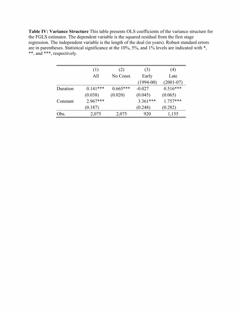
Table IV: Variance Structure This table presents OLS coefficients of the variance structure for the FGLS estimator. The dependent variable is the squared residual from the first stage regression. The independent variable is the length of the deal (in years). Robust standard errors are in parentheses. Statistical significance at the 10%, 5%, and 1% levels are indicated with *, **, and ***, respectively.

(1) (2) (3) (4)

All No Const. Early Late

(1994-00) (2001-07)

Duration 0.141*** 0.665*** -0.027 0.516***

(0.038) (0.020) (0.045) (0.065) Constant 2.967*** 3.361*** 1.757*** (0.187) (0.248) (0.282) Obs. 2,075 2,075 920 1,155

Table V Log-return CAPM: This table shows regression coefficients from the second step of the FGLS estimator. Panel A shows standard FGLS estimates where the second step is estimated using OLS. Panel B shows a modified FGLS estimator where the second step is estimated using a Tobit regression that is robust to the left-truncation of the log-return. The dependent variable is the normalized excess log-return of each deal. The independent variables are a constant term (Gamma), a normalized constant term (Constant), and the normalized excess log-return on the market (Beta). Robust standard errors are in parentheses. Statistical significance at the 10%, 5%, and 1% levels are indicated with *, **, and ***, respectively. Panel A: FGLS Specification

(1) (2) (3) (4)

All All Early Late

(1994-00) (2001-07)

Constant -0.046*** 0.041** 0.107*** -0.013

(0.009) (0.017) (0.022) (0.029)

Gamma

-0.471*** -0.934*** -0.103

(0.070) (0.128) (0.106)

Beta 2.417*** 2.278*** 2.258*** 1.873*** (0.160) (0.157) (0.235) (0.250) Obs. 2,075 2,075 920 1,155

Panel B: Tobit Specification

(1) (2) (3) (4)

All All Early Late

(1994-00) (2001-07) Constant -0.089*** 0.048** 0.145*** -0.047

(0.011) (0.022) (0.029) (0.036) Gamma -0.738*** -1.353*** -0.213

(0.103) (0.160) (0.144) Beta 2.934*** 2.758*** 2.750*** 2.342***

(0.203) (0.204) (0.311) (0.305) Obs. 2,075 2,075 920 1,155

Table VI: Beta Estimates Using Simulated Deal Data For each alpha and beta choice, we construct 100 datasets. Each dataset contains 150 funds, each of which has 20 deals. The performance of each deal is simulated using the jump-CAPM model with the remaining parameters equal to their estimated values (γ = −0.5 , σ 2 = 0.141, and σ J

2 = 2.967 ). The length of each deal is drawn from the empirical distribution in Figure 2 (conditional on the deal exiting prior to the termination of the fund). The vintage year of each fund is drawn uniformly from 1980 to 2000. The market return and risk-free rates are actual historical rates. For each of the 100 datasets, we estimate the beta coefficients using five different empirical models: Gross-IRR, Net-IRR, Static-CAPM, log-return CAPM (log-CAPM), and jump-CAPM, as described in the text. The table reports the average and standard deviation of the resulting 100 estimated beta coefficients. The case with alpha and beta parameters closest to their empirical counterparts is highlighted in bold.

True Alpha

True Beta Gross IRR Net IRR

Static CAPM log-CAPM

Jump-CAPM

0% 0.0 -0.163 -0.613 -0.203 -0.015 -0.008 (2.37) (4.99) (0.11) (0.13) (0.12)

10% 0.0 -0.044 0.025 0.098 0.001 0.009 (1.37) (1.45) (0.11) (0.12) (0.12)

20% 0.0 -0.085 -0.078 0.374 -0.009 -0.003 (1.64) (1.42) (0.11) (0.12) (0.12)

0% 1.0 0.379 -1.452 0.805 1.012 1.018 (2.81) (5.02) (0.11) (0.12) (0.12)

10% 1.0 1.055 0.785 1.090 0.993 1.001 (1.12) (1.45) (0.11) (0.12) (0.12)

20% 1.0 1.082 0.898 1.369 0.978 0.985 (2.30) (2.26) (0.12) (0.12) (0.12)

0% 2.0 1.120 -1.450 1.777 2.092 2.101 (3.47) (4.90) (0.11) (0.12) (0.12)

10% 2.0 1.800 1.336 2.064 2.081 2.089 (1.84) (2.41) (0.11) (0.12) (0.12)

20% 2.0 2.236 2.076 2.351 2.045 2.054 (1.75) (1.46) (0.12) (0.12) (0.12)