Almut Gassmann Meteorological Institute of the University ...
31
Split explicit methods Almut Gassmann Meteorological Institute of the University of Bonn Germany St.Petersburg Summer School 2006 on nonhydrostatic dynamics and fine scale data assimilation
Transcript of Almut Gassmann Meteorological Institute of the University ...

Split explicit methods
Almut Gassmann
Meteorological Institute of the University of Bonn
Germany
St.Petersburg Summer School 2006 on nonhydrostatic dynamics and fine scale data assimilation

Two common methods applied to nonhydrostatic compressible equations
Semi-Implicit/Semi-Lagrange
Split-Explicit
completely implicit fast waves horizontally explicit vertically implicit
Poisson equation time stepping fractional steps
Lagrangian advection Eulerian
large time steps possible advantages straightforward numericsdo well on parallel platforms
terrainfollowing coords difficulties numerical stabilitychoice of basic state proper splitting of terms
2

1) How to divide the terms into slow and fast ones? 2) How to couple slow and fast processes tightly? 3) How to ensure numerical stability? 4) How to define the advection algorithm?
Split explicit methods
Klemp/Wilhelmson
Euler forward
Wicker/Skamarock
Gassmann
3

Divide equations into slow and fast parts – Investigate fast modes
Linear wave analysis of...
...gives us the dispersion relation for acoustic and gravity waves...
...wherein these both modes are coupled via the divergence.
As a consequence the acoustic and gravity modes are not strictly separable.But this was ignored in the past by the pioneers in this working field.
4
Numerical stability analysis of (LM-equations) ...
critical points concerning LM / MM5
terms for divergence damping
5
Divide equations into slow and fast parts – Investigate fast modes
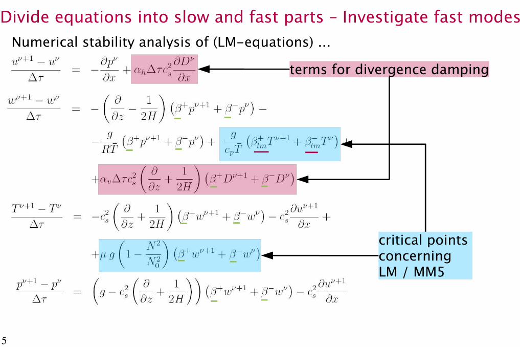
...yields a matrix equation like
...and an amplification matrix
...whose eigenvalues must not exceed 1 for numerical stability.
But...If the temperature part of the buoyancy term are treated explicitly for an isothermal atmosphere, the gravity waves become unstable!
gravity waves
sound waves
explicit
implicit
both curves coincide
6
Divide equations into slow and fast parts – Investigate fast modes

For the correct representation of the actual stability (N²),the vertical advection of pressure and temperature is required
in the fast waves part.
Dropping vertical advectionof T with nonisothermalreference state. (LM pathology)
Vertical advection of T and p'is performed with the nonisothermal reference state.
N²=0.0001/s² N²=0.0001/s²
7
Divide equations into slow and fast parts – Investigate fast modes

As we shall see, some damping of sound waves is required in the splitting scheme...
Divergence damping in thehorizontal momentum equations
Divergence damping in all three momentum equations
Off-centered implicit weights (β+=0.7)
8
Divide equations into slow and fast parts – Investigate fast modes

Divergence damping analysis
Isotropic divergence damping
damping coefficient
Sound waves are damped.Gravity waves remain
unmodified.
Horizontal divergence damping
Sound waves are damped proportionallyto the horizontal wave number.
Gravity waves are altered in phaseand become faster or slower.
9
Divide equations into slow and fast parts – Investigate fast modes
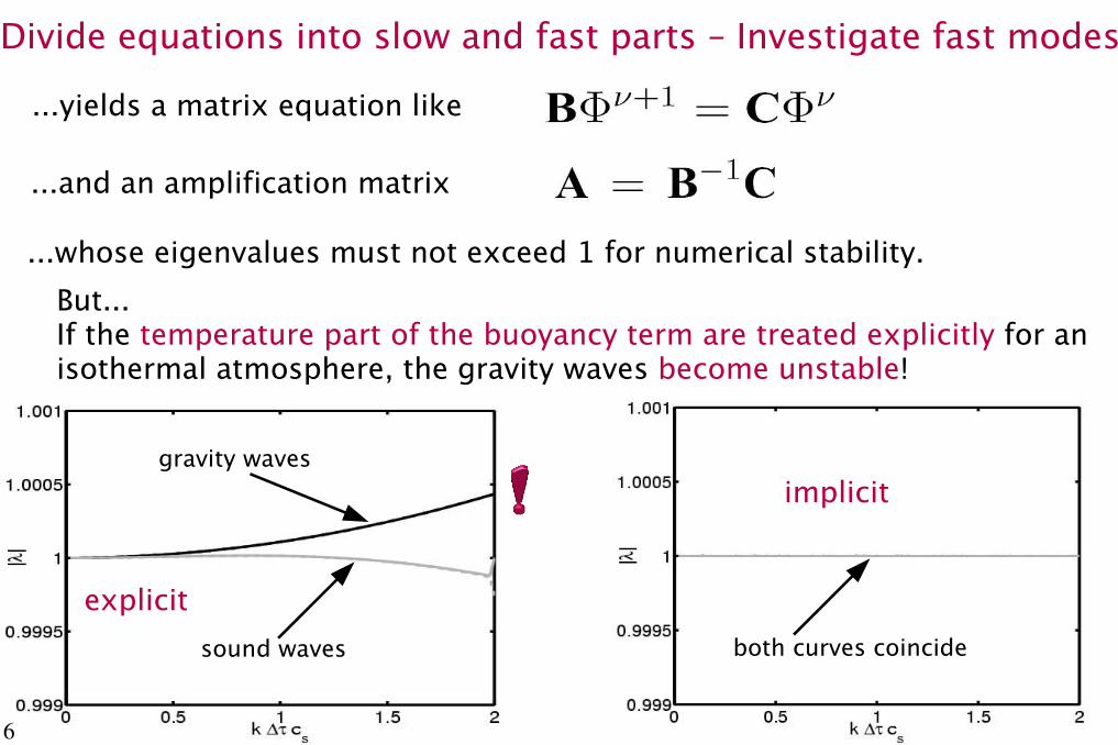
Conclusions from this section
●Numerical stability is required for fast waves part alone.
●A horizontally forward-backward explicit and vertically implicit numerical scheme is applied.
●Acoustic and gravity modes are coupled via the divergence and, therefore, are not separable.
●All terms relevant for vertical structure and wave propagation must be treated within the fast waves part and with the same implicity weights.
●Divergence damping should only be used if it is applied to all three momentum equations. Off-centering the implicity weights is an altenative damping mechanism.
10
Divide equations into slow and fast parts – Investigate fast modes

Numerical analysis of the sound advection system
fast modessound waves
slow modesadvection terms
For comparison of different schemes we must define a common advection scheme:Runge-Kutta 2nd order in time and 3rd order in space.
Klemp/Wilhelmson
Euler forward
Wicker/Skamarock
Gassmann
11

Numerical analysis of the sound advection system
RK2-Advection (Runge-Kutta 2nd order in time)
3rd order in space (for U>0)
Example: Euler scheme
Fourier representation in space dimensionless wavenumber
Courant number for advection
Imaginary part is negative and leads to damping
12

Numerical analysis of the sound advection systemThe computations are performedon a staggered C-grid with forward--backward differencing for the fast waves part and the commonly defined advection algorithm.
Number of small time steps perlarge step: N=4u=0.75,cs=3,dx=dt=1 arenondimensional numbers
Euler forward
Wicker/Skamarock Gassmann
First 8 time steps
13

Numerical analysis of the sound advection systemExpansion of the squared eigenvalues of the amplification matrix:
wavenumber for the advection schemereal part: phase characteristicimaginary part (is negative): damping
Splitting error term Higher order terms
Euler forward
Gassmann
Wicker/Skamarock
Courant numbers
14

Numerical analysis of the sound advection system
Stability diagrams for an 8 Δx wave
Euler forward Wicker/Skamarock Gassmann
Forward moving mode
Backward moving mode
with divergence damping
unstable
damped
15

Splitting scheme analysis with the linear nonhydrostaticcompressible system
Stability diagrams of the Gassmann scheme
no divergence damping,no offcentering of implicit weights
unstable
no divergence damping,off-centering of implicit weights
isotropic divergence damping,no off-centering of implicit weights
stable
stablestable
16

Splitting schemes - Conclusions
●Though the advection scheme and the fast-waves scheme may be stable for themselves, the combination in the splitting scheme is not automatically stable!
●The splitting error term is a multiplicative combination of both parts and contains the significant propagation information, and so never vanishes: it may only be reduced.
●An additional damping mechanism (hidden in H.O.T.) is essential.
●The propagation of waves in different directions (modes) is either amplified or damped.
●The Gassmann-scheme is shown to be the best compromise among the candidates presented.
●The stability analysis of the splitting scheme for the complete nonhydrostatic compressible equations yields satisfactory results.
17

n n+1n**n*
A gravity wave generatoris situated in the center ofthe domain, the ambienthorizontal wind increaseswith height from 5 to 15m/s.
Strang
Klemp/Wilhelmson
From Durran (1999)
Since the operators for each fractional step do not commute, the stability of each individual operator no longer guarantees the stability of the overall scheme.
Other variants of splitting schemes – Strang splitting
18

Other variants of splitting schemes – Runge Kutta type advection
Runge-Kutta-2nd order in time Runge-Kutta-3rd order in time
Larger Courantnumbers for RK3 and higher accuracy in space!
But the Gassmannscheme is independentof the actual advection scheme and may be combined with RK3.
From Wicker and Skamarock (2002), cf. also WRF-Documentation19

Applications – Consequences for the LM
The nonhydrostatic compressible LM (Lokal-Modell) is the operational regional forecast model of the COSMO group. Its dynamical core reads:
usual contravariant vertical velocity vertical velocity related to the terrain following coordinates
20

Applications – Consequences for the LM
vertical advection of T and p' in slow modes vertical advection of T and p' in fast modes
Schaer test case with Gassmann-splitting
21

Applications – Consequences for the LM
With the new fast waves algorithm all information for gravity waves is included in the fast-waves part. That is the prerequisite for applying the radiative upper boundary condition directly in the vertical implicit solver of the fast-waves.
Radiative upper boundary condition - RUBC
relation for hydrostatic gravity waves at the model top
22
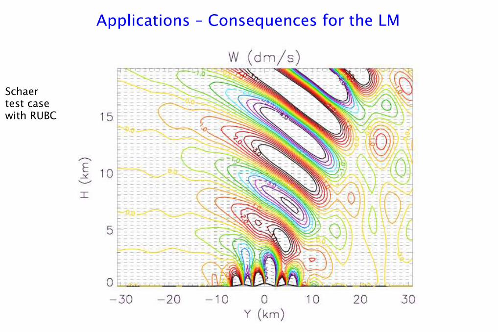
Applications – Consequences for the LM
Schaer test case with RUBC

Applications – Consequences for the LM
Schaer test case withsponge upperboundary condition

Applications – Consequences for the LM Applications – Consequences for the LM Applications – Consequences for the LM
Schaer test case withsponge upperboundary condition
old LMdynamics

Applications – Consequences for the LM
Nonlinear flow past a high mountain, dx=7km,tropopause at 10km, realistic vertical levels
withRadiative Upper Boundary Condition
26

Ap
plica
tions
– C
onse
quen
ces
for
the
LM
Old
LM
dyn
amic
s.W
ithout
and w
ith d
ynam
ic
low
er b
oundar
y co
ndit
ion
in t
he
hori
zonta
l m
om
entu
m e
quat
ions.
New
LM
dyn
amic
s.W
ith s
ponge
laye
r an
d w
ith R
UBC
.
Resting atmosphere over a high mountain
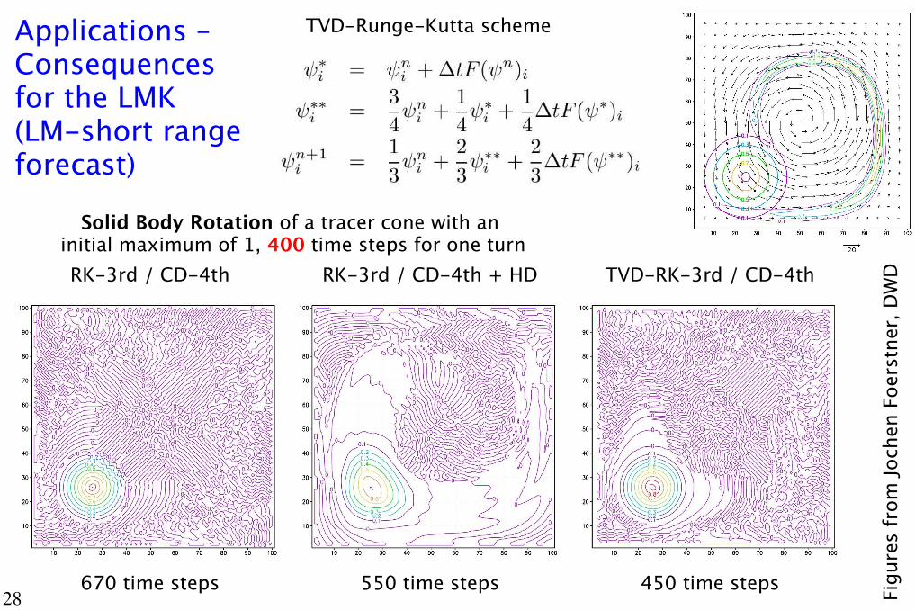
Applications – Consequences for the LMK (LM-short range forecast)
TVD-Runge-Kutta scheme
RK-3rd / CD-4th RK-3rd / CD-4th + HD TVD-RK-3rd / CD-4th
670 time steps 550 time steps 450 time steps
Solid Body Rotation of a tracer cone with an initial maximum of 1, 400 time steps for one turn
Figure
s fr
om
Joch
en F
oer
stner
, D
WD
28

Applications – Consequences for the LMK (LM-short range forecast)
TVD-Runge-Kutta schemenow applied within the
framework of the Wicker/Skamarock-splitting
advection of a tracerwithout fast-waves
TVD-RK3/5th upwind
TVD-RK3/4thCDTVD-RK3/4thCD
+horizontal diffusion TVD-RK3/5thupwind
Figure
s fr
om
Joch
en F
oer
stner
, D
WD
29

Applications – Conservative split-explicit WRF version
Flux quantities
Flux form equations
How to linearize these equations for splitting off the fast-waves part?
This corresponds to a linearization around the present time step t.
slow modes
fast modes
WRF - Weather Research and Forecasting modeling systemcollaboration amongst NCAR, NOAA, FSL, AFWA, NRL, CAPS, FAA in the U.S.A.
From Klemp et al., 2000,cf. also Skamarock et al.2005
30

Summary on split-explicit methods
●The split explicit method is an efficient and accurate method for integrating the unfiltered hydro-thermodynamic equations.
●The method is easily implemented also on parallel platforms.
●Numerical stability is the crucial point in designing split-explicit schemes.
●Another problem is the proper mode splitting.
●The combination with different advection schemes is possible.
●Split-explicit time integration is even applicable to the flux-form equations.
●Features like the radiative upper boundary condition are easily included in the complete algorithm.
31