Almost Sure Stability and Stabilization for Hybrid ... · PDF fileHua Yang,1,2 Huisheng Shu,3...

Hindawi Publishing CorporationMathematical Problems in EngineeringVolume 2012, Article ID 183729, 21 pagesdoi:10.1155/2012/183729

Research ArticleAlmost Sure Stability and Stabilization for HybridStochastic Systems with Time-Varying Delays

Hua Yang,1, 2 Huisheng Shu,3 Xiu Kan,1 and Yan Che1

1 School of Information Science and Technology, Donghua University, Shanghai 200051, China2 College of Information Science and Engineering, Shanxi Agricultural University, Taigu 030801, China3 Department of Applied Mathematics, Donghua University, Shanghai 200051, China

Correspondence should be addressed to Huisheng Shu, [email protected]

Received 21 June 2012; Accepted 1 August 2012

Academic Editor: Bo Shen

Copyright q 2012 Hua Yang et al. This is an open access article distributed under the CreativeCommons Attribution License, which permits unrestricted use, distribution, and reproduction inany medium, provided the original work is properly cited.

The problems of almost sure (a.s.) stability and a.s. stabilization are investigated for hybridstochastic systems (HSSs)with time-varying delays. The different time-varying delays in the driftpart and in the diffusion part are considered. Based on nonnegative semimartingale convergencetheorem, Holder’s inequality, Doob’s martingale inequality, and Chebyshev’s inequality, somesufficient conditions are proposed to guarantee that the underlying nonlinear hybrid stochasticdelay systems (HSDSs) are almost surely (a.s.) stable. With these conditions, a.s. stabilizationproblem for a class of nonlinear HSDSs is addressed through designing linear state feedbackcontrollers, which are obtained in terms of the solutions to a set of linearmatrix inequalities (LMIs).Two numerical simulation examples are given to show the usefulness of the results derived.

1. Introduction

In the past decades, the problems of stability analysis and stabilization synthesis of stochasticsystems have received significant attentions, and many results have been reported; see, forexample [1–7] and the references therein. Commonly, the above problems can be solved notonly in moment sense [8–10] but also in a.s. sense [11, 12]. However, in recent years, muchinterest has been focused on a.s. stability problems for stochastic systems; see, for example[8, 13] and the references therein.

It is well known that a lot of dynamical systems have variable structures subjectto abrupt changes in their parameters, which are usually caused by abrupt phenomenasuch as component failures or repairs, changing subsystem interconnections, and abruptenvironmental disturbances. The HSSs, which are regarded as the stochastic systems with

2 Mathematical Problems in Engineering

Markovian switching in this paper, have been used to model the previous phenomena; see,for example [14–18] and the references therein. The HSSs combine a part of the state x(t) thattakes values in R

n continuously and another part of the state r(t) that is a Markov chaintaking discrete values in a finite space S = {1, 2, . . . ,N}. One of the important issues inthe study of HSSs is the analysis of stability. In particular, it is not necessary for the stableHSSs to require every subsystem to be stable; in other words, even all the subsystems areunstable; as the result of Markovian switching, the HSSs may be stable. These reveal that theMarkovian jumps play an important role in the stability analysis of HSSs. Therefore, in thepast few decades, a great deal of literature has appeared on the topic of stability analysis andstabilization synthesis of HSSs; see, for example [2, 13, 14, 19, 20].

On the other hand, time delays are frequently encountered in a variety of dynamicsystems, such as nuclear reactors, chemical engineering systems, biological systems, andpopulation dynamics models. They are often a source of instability and poor performance ofsystems. So the problems of stability analysis and stabilization synthesis of HSDSs have beenof great importance and interest. The classical efforts can be classified into two categories,namely, moment sense criteria, see, for example [21–23], and a.s. sense criteria, see, forexample [24, 25]. Among the existing results, in [25], based on the techniques proposed in[26] which were developed via the results of [11], a.s. stability and stabilization of HSDSswere studied. In [24], the a.s. stability analysis problem for a general class of HSDSs wasderived from extending the results in [25] to HSSs with mode-dependent interval delays.However, to the author’s best knowledge, when the different time-varying delays in thedrift part and in the diffusion part are considered, the a.s. stability analysis and stabilizationsynthesis problems for nonlinear HSDSs have not been adequately addressed and remain aninteresting and challenging research topic. This situation motivates the present study.

In this paper, we are concerned with a.s. stability analysis and stabilization synthesisproblems for HSDSs. The purpose of stability is to develop conditions such that theunderlying systems are a.s. stable. Following the same idea as in dealing with the stabilityproblem, linear state feedback controllers are designed such that the special nonlinear orlinear closed-loop systems are a.s. stable. The explicit expressions for the desired statefeedback controllers are given by means of the solutions to a set of LMIs. Two numericalsimulation examples are exploited to verify the effectiveness of the theoretical results. Themain contribution of this paper is mainly twofold: (1) the different time-varying delays in thedrift part and in the diffusion part are considered for nonlinear HSDSs; (2) for a class of nonlinearHSDSs, the stabilization synthesis problem is investigated in the a.s. sense.

This paper is organized as follows. In Section 2, we formulate some preliminaries.In Section 3, we investigate the a.s. stability for the hybrid stochastic systems with time-varying delays. In Section 4, the results of Section 3 are then applied to establish a sufficientcriterion for the stabilization. In Section 5, two examples are discussed for illustration. Finally,conclusions are drawn in Section 6.

Notation 1. The notation used here is fairly standard unless otherwise specified. Rn and Rn×m

denote, respectively, the n dimensional Euclidean space and the set of all n ×m real matrices,and letR+ = [0,+∞). (Ω,F, {Ft}t≥0,P) be a complete probability space with a natural filtration{Ft}t≥0 satisfying the usual conditions (i.e., it is right continuous, and F0 contains all P-nullsets). If x, y are real numbers, then x ∨ y stands for the maximum of x and y, and x ∧ y theminimum of x and y. MT represents the transpose of the matrix M. λmax(M) and λmin(M)denote the largest and smallest eigenvalue ofM, respectively. | · | denotes the Euclidean normin R

n. E{·} stands for the mathematical expectation. P{·}means the probability. C([−τ, 0];Rn)

Mathematical Problems in Engineering 3

denotes the family of all continuous Rn-valued function ϕ on [−τ, 0] with the norm |ϕ| =

sup{|ϕ(θ)| : −τ ≤ θ ≤ 0}. CbF0([−τ, 0);Rn) being the family of all F0-measurable bounded

C([−τ, 0);Rn)-value random variables ξ = {ξ(θ) : −τ ≤ θ ≤ 0}. L1(R+;R+) denotes the familyof functions λ : R+ → R+ such that

∫∞0 λ(t)dt < ∞.

2. Problem Formulation

In this paper, let r(t), t ≥ 0 be a right-continuousMarkov chain on the probability space takingvalues in a finite state space S = {1, 2, . . . ,N}with generator Γ = (γij)N×N given by

P{r(t + Δ) = j | r(t) = i

}=

{γijΔ + o(Δ) if i /= j,

1 + γiiΔ + o(Δ) if i = j,(2.1)

whereΔ > 0 and γij ≥ 0 is the transition rate frommode i tomode j if i /= j while γii = −∑j /= i γij .Assume that the Markov chain r(·) is independent of the Brownian motion B(·). It is knownthat almost all sample paths of r(·) are right-continuous step functions with a finite numberof simple jumps in any finite subinterval of R+ := [0,∞).

Let us consider a class of stochastic systems with time-varying delays:

dx(t) = f(x(t), x(t − τ1(t)), t, r(t))dt + g(x(t), x(t − τ2(t)), t, r(t))dB(t) (2.2)

with initial data x0 = {x(θ) : −τ ≤ θ ≤ 0} = ξ ∈ CbF0([−τ, 0);Rn) and r(0) = r0 ∈ S, where

τ � max{τ1, τ2}, τ1 and τ2 are positive constant and τ1(t) and τ2(t) are nonnegative differentialfunctions which denote the time-varying delays and satisfy

0 ≤ τ1(t) ≤ τ1, τ1(t) ≤ dτ1 < 1,

0 ≤ τ2(t) ≤ τ2, τ2(t) ≤ dτ2 < 1.(2.3)

The nonlinear functions f : Rn × R

n × R+ × S → Rn and g : R

n × Rn × R+ × S → R

n×m satisfythe local Lipschitz condition in (x, y, z); that is, for any K > 0, there is LK > 0 such that

∣∣f(x, y, t, i

) − f(x, y, t, i

)∣∣ ∨ ∣∣g(x, z, t, i) − g(x, z, t, i)∣∣

≤ LK

(|x − x| + ∣∣y − y∣∣ + |z − z|),

(2.4)

for all |x| ∨ |y| ∨ |z| ∨ |x| ∨ |y| ∨ |z| ≤ K, t ≥ 0 and i ∈ S, and moreover, supt≥0,i∈S{|f(0, 0, t, i)| ∨|g(0, 0, t, i)| : t ≥ 0, i ∈ S} ≤ K0 with some nonnegative number K0.

Remark 2.1. It should be pointed out that the systems (2.2) can be seen as the specializationof multiple time-varying delays systems which are of the form

dx(t) = f(x(t), x(t − τ1(t)), x(t − τ2(t)), t, r(t))dt

+ g(x(t), x(t − τ1(t)), x(t − τ2(t)), t, r(t))dB(t).(2.5)


But it is easy to see that the results in this paper can be applied to the systems (2.5) by thesimilar assumption in (2.4).

Let C2,1(Rn × R+ × S;R+) denote the family of all nonnegative functions V (x, t, i) onR

n ×R+ × S that are twice continuously differentiable in x and once in t. If V ∈ C2,1(Rn ×R+ ×S;R+), define an operator L associated with (2.2) from R

n × Rn × R

n × R+ × S to R by

LV(x, y, z, t, i

)= Vt(x, t, i) + Vx(x, t, i)f

(x, y, t, i

)

+12trace

[gT (x, z, t, )Vxx(x, t, i)g(x, z, t, i)

]+

N∑

j=1

γijV(x, t, j

).

(2.6)

Remark 2.2. LV is thought as a single notation and is defined on Rn × R

n × Rn × R+ × Swhile

V is defined on Rn × [−τ,∞) × S.

Definition 2.3. The system (2.2) is said to be a.s. stable if for all ξ ∈ CbF0([−τ, 0);Rn) and r0 ∈ S

P

(limt→∞

x(t; ξ, r0) = 0)

= 1. (2.7)

3. Main Results

Theorem 3.1. Assume that there exist nonnegative functions V ∈ C2,1(Rn × R+ × S;R+), λ ∈L1(R+;R+), ω1, ω2, ω3 ∈ C(Rn;R+) such that

LV(x, y, z, t, i

) ≤ λ(t) − k1ω1(x) + k2ω2(y)+ k3ω3(z),

∀(x, y, z, t, i) ∈ Rn × R

n × Rn × R+ × S,

(3.1)

ω1(x) > ω2(x) +ω3(x), ∀x /= 0, (3.2)

lim|x|→∞

inft≥0,i∈S

V (x, t, i) = ∞, (3.3)

where k1, k2 and k3 are positive numbers satisfying k1 ≥ max{k2/(1 − dτ1), k3/(1 − dτ2)}. Thensystem (2.2) is almost surely stable.

To prove this theorem, let us present the following lemmas.

Lemma 3.2 (see [24, 25]). If V ∈ C2,1(Rn × R+ × S;R+), then for any t ≥ 0, the generalized Ito’sformula is given as

dV (x(t), t, r(t)) = LV (x(t), x(t − τ1(t)), x(t − τ2(t)), t, r(t))dt

+ Vx(x(t), t, r(t))g(x(t), x(t − τ2(t)), t, r(t))dB(t)

+∫

R

[V (x(t), t, r(t) + l(r(t), α)) − V (x(t), t, r(t))] × μ(dt, dα),

(3.4)

where function l(·, ·) and martingale measure μ(·, ·) are defined as, for example, (2.6) and (2.7) in [25].


Lemma 3.3 (see [27]). Let A1(t) and A2(t) be two continuous adapted increasing processes ont ≥ 0 with A1(0) = A2(0) = 0 a.s., let M(t) be a real-valued continuous local martingale withM(0) = a.s., and let ζ be a nonnegative F0-measurable random variable such that Eζ < ∞. DenoteX(t) = ζ +A1(t) −A2(t) +M(t) for all t ≥ 0. If X(t) is nonnegative, then

{limt→∞

A1(t) < ∞}

⊂{limt→∞

X(t) < ∞}∩{limt→∞

A2(t) < ∞}

a.s., (3.5)

where C ⊂ D a.s. means P(C ∩Dc = 0) = 0. In particular, if limt→∞A1(t) < ∞ a.s., then,

limt→∞

X(t) < ∞, limt→∞

A2(t) < ∞, −∞ < limt→∞

M(t) < ∞ a.s.. (3.6)

That is, all of the three processes X(t), A2(t), and M(t) converge to finite random variableswith probability one.

Lemma 3.4 (see [25]). Under the conditions of Theorem 3.1, for any initial data {x(θ) : −τ ≤ θ ≤0} = ξ ∈ Cb

F0([−τ, 0);Rn) and r(0) = i0 ∈ S, (2.2) has a unique global solution.

Proof. Fix any initial data ξ, r0, and let β be the bound for ξ. For each integer k ≥ β, define

f (k)(x, y, t, i)= f

(|x| ∧ k

|x| x,

∣∣y∣∣ ∧ k∣∣y∣∣ y, t, i

)

, (3.7)

where we set (|x| ∧ k/|x|)x = 0 when x = 0. Define g(k)(x, z, t, i) similarly. By (2.4), wecan observe that f (k) and g(k) satisfy the global Lipschitz condition and the linear growthcondition. By the known existence-and-uniqueness theorem, there exists a unique globalsolution xk(t) on t ∈ [−τ,∞) to the equation

dxk(t) = f (k)(xk(t), xk(t − τ1(t)), t, r(t))dt

+ g(k)(xk(t), xk(t − τ2(t)), t, r(t))dB(t)(3.8)

with initial data {xk(θ) : −τ ≤ θ ≤ 0} = ξ and r(0) = r0.Define the stopping time

σk = inf{t ≥ 0 : |xk(t)| ≥ k}, (3.9)

where we set inf ∅ = ∞ as usual. It is easy to show that xk(t) = xk+1(t) if 0 ≤ t ≤ σk, whichimplies that σk is increasing in k. Letting σ = limk→∞σk, the property above also enables usto define x(t) for t ∈ [−τ, σ) as x(t) = xk(t) if −τ ≤ t ≤ σk.


It is clear that x(t) is a unique solution of (2.2) for t ∈ [−τ, σ). To complete the proof,we only need to show P{σ = ∞} = 1. By Lemma 3.2, we have that for any t > 0,

EV (xk(t ∧ σk), t ∧ σk, r(t ∧ σk)) = EV (xk(0), 0, r(0))

+ E

∫ t∧σk

0L(k)V (xk(s), xk(s − τ1(s)), xk(s − τ2(s)), s, r(s))ds,

(3.10)

where operator L(k)V is defined similarly as LV was defined by (2.6). By the definitions off (k) and g(k), if 0 ≤ s ≤ t ∧ σk, we hence observe that

L(k)V (xk(s), xk(s − τ1(s)), xk(s − τ2(s)), s, r(s))

= LV (xk(s), xk(s − τ1(s)), xk(s − τ2(s)), s, r(s)).(3.11)

By the conditions of (3.1) and (3.2), we derive that

EV (xk(t ∧ σk), t ∧ σk, r(t ∧ σk))

≤ V (ξ(0), 0, r0) + E

∫ t

0[−k1ω1(x(s)) + k2ω2(x(s − τ1(s))) + k3ω3(x(s − τ2(s)))]ds

+∫ t

0λ(s)ds

≤ V (ξ(0), 0, r0) + E

∫ t

0−k1ω1(x(s))ds + E

∫ t−τ1(t)

−τ1

(k2

1 − dτ1

)ω2(s)ds

+ E

∫ t−τ2(t)

−τ2

(k3

1 − dτ2

)ω3(s)ds +

∫ t

0λ(s)ds

≤ V (ξ(0), 0, r0) + E

∫0

−τk1[ω2(ξ(θ)) +ω3(ξ(θ))]dθ

− E

∫ t

0k1(ω1(s) −ω2(s) −ω3(s))ds +

∫ t

0λ(s)ds

≤ V (ξ(0), 0, r0) + E

∫0

−τk1[ω2(ξ(θ)) +ω3(ξ(θ))]dθ +

∫ t

0λ(s)ds.

(3.12)

On the other hand,

EV (xk(t ∧ σk), t ∧ σk, r(t ∧ σk)) ≥∫

{σk≤t}V (xk(t ∧ σk), t ∧ σk, r(t ∧ σk))dP

≥ P{σk ≤ t} inf|x|≥k,t≥0,i∈S

V (x, t, i).(3.13)


This yields

P{σk ≤ t} ≤ V (ξ(0), 0, r0) + E∫0−τ k1[ω2(ξ(θ)) +ω3(ξ(θ))]dθ +

∫ t0 λ(s)ds

inf|x|≥k,t≥0,i∈SV (x, t, i). (3.14)

Letting k → ∞ and using (3.3), we obtain P(σ ≤ t) = 0. Since t is arbitrary, we musthave P(σ = ∞) = 1. The proof is therefore complete.

Let us now begin to prove our main result.

Proof. Let ω(x) = ω1(x) − ω2(x) − ω3(x) for all x ∈ Rn. Inequality (3.2) implies ω(x) > 0

whenever x /= 0. Fix any initial value ξ and any initial state r0, and for simplicity writex(t; ξ, r0) = x(t).

By Lemma 3.2 and condition (3.1), we have

V (x(t), t, r(t)) = V (ξ(0), 0, r0) +∫ t

0LV (x(s), x(s − τ1(s)), x(s − τ2(s)), s, r(s))ds

+∫ t

0Vx(x(s), s, r(s))g(x(s), x(s − τ2(s)), s, r(s))dB(s)

+∫ t

0

∫

R

[V (x(s), s, r0 + l(r(s), α)) − V (x(s), s, r(s))]μ(ds, dα)

≤ V (ξ(0), 0, r0) +∫ t

0λ(s)ds −

∫ t

0k1ω1(x(s))

+∫ t

0[k2ω2(x(s − τ1(s))) + k3ω3(x(s − τ2(s)))]ds

+∫ t


+∫ t

0

∫

R

[V (x(s), s, r0 + l(r(s), α)) − V (x(s), s, r(s))]μ(ds, dα)

≤ V (ξ(0), 0, r0) +∫ t

0λ(s)ds + k1

∫0

−τ[ω2(x(s)) +ω3(x(s))]ds

− k1

∫ t

0ω(x(s))ds +

∫ t


+∫ t

0

∫

R

[V (x(s), s, r0 + l(r(s), α)) − V (x(s), s, r(s))]μ(ds, dα).

(3.15)


Since∫∞0 λ(s)ds < ∞, applying Lemma 3.3 we obtain that

limt→∞

∫ t

0ω(x(s))ds =

∫∞

0ω(x(s))ds < ∞ a.s., (3.16)

limt→∞

supV (x(t), t, r(t)) < ∞ a.s.. (3.17)

Define β : R+ → R+ as β(r) = inf|x|≥r,0≤t<∞,i∈SV (x, t, i). Then, it is obvious to see from (3.17)that

sup0≤t<∞

β(|x(t)|) ≤ sup0≤t<∞

V (x(t), t, r(t)) < ∞ a.s.. (3.18)

On the other hand, by (3.3)we have sup0≤t<∞|x(t)| < ∞ a.s.. It is easy to find an integerk0 such that |ξ| < k0 a.s. because of ξ ∈ Cb

F0([−τ, 0);Rn). Furthermore, for any integer k > k0,

we can define the stopping time

ρk = inf{t ≥ 0 : |x(t)| ≥ k}, (3.19)

where inf ∅ = ∞ as usual. Clearly, ρk → ∞ a.s. as k → ∞. Moreover, for any given ε > 0,there is kε ≥ k0 such that P{ρk < ∞} ≤ ε for any k ≥ kε.

It is straightforward to see from (3.16) that limt→∞ infω(x(t)) = 0 a.s.; then we claimthat

limt→∞

ω(x(t)) = 0 a.s.. (3.20)

The rest of the proof is carried out by contradiction. That is, assuming that (3.20) isfalse, we have

P

{limt→∞

supω(x(t)) > 0}

> 0. (3.21)

Furthermore, there exist ε0 > 0 and ε > ε1 > 0 such that

P(σ2j < ∞ : j ∈ Z

) ≥ ε0, (3.22)

where Z is a set of natural numbers and {σj}j≥1 are a sequence of stopping times defined by

σ1 = inf{t ≥ 0 : ω(x(t)) ≥ 2ε1},σ2j = inf

{t ≥ σ2j−1 : ω(x(t)) ≤ ε1

}, j = 1, 2, . . . ,

σ2j+1 = inf{t ≥ σ2j : ω(x(t)) ≤ 2ε1

}, j = 1, 2, . . . .

(3.23)


By the local Lipschitz condition (2.4), for any given k > 0, there exists Lk > 0 such that

∣∣f(x, y, t, i

)∣∣ ∨ ∣∣g(x, z, t, i)∣∣ ≤ Lk, (3.24)

for all |x| ∨ |y| ∨ |z| ≤ k, t ≥ 0 and i ∈ S.For any j ∈ Z, let T < σ2j − σ2j−1; by Holder’s inequality and Doob’s martingale

inequality, we compute

E

{

I{σ2j<ρk} sup0≤t≤T

∣∣x(σ2j−1 + t

) − x(σ2j−1

)∣∣2}

= E

⎧⎨

⎩I{σ2j<ρk} sup

0≤t≤T

∣∣∣∣∣

∫σ2j−1+t

σ2j−1f(x(s), x(s − τ1(s)), s, r(s))ds

+∫σ2j−1+t

σ2j−1g(x(s), x(s − τ2(s)), s, r(s))dB(s)

∣∣∣∣∣

2⎫⎬

⎭

≤ 2E

⎧⎨

⎩I{σ2j<ρk} sup

0≤t≤T

∣∣∣∣∣

∫σ2j−1+t

σ2j−1f(x(s), x(s − τ1(s)), s, r(s))ds

∣∣∣∣∣

2⎫⎬

⎭

+ 8E

{

I{σ2j<ρk} sup0≤t≤T

∫σ2j−1+t

σ2j−1

∣∣g(x(s), x(s − τ2(s)), s, r(s))∣∣2ds

}

≤ 2L2kT(T + 4),

(3.25)

where IA is the indicator of set A.Since ω(x) is continuous in R

n, it must be uniformly continuous in the closed ballSk = {x ∈ R

n : |x| ≤ k}. For any given b > 0, we can choose cb > 0 such that |ω(x) −ω(y)| < b

whenever x, y ∈ Sk and |x − y| < cb. Furthermore, let us choose

ε =ε03, k ≥ kε, b = ε1. (3.26)

By inequality (3.25) and Chebyshev’s inequality, we have

P({

ρk ≤ σ2j})

+ P

({σ2j < ρk

} ∩{

sup0≤t≤T

∣∣ω(x(σ2j−1 + t

)) −ω(x(σ2j−1

))∣∣ ≥ ε1

})

≤ P({

ρk ≤ σ2j} ∩ {σ2j = ∞})

+ P({

ρk ≤ σ2j} ∩ {σ2j < ∞})

+ P

({σ2j < ρk

} ∩{

sup0≤t≤T

∣∣x(σ2j−1 + t

) − x(σ2j−1

)∣∣ ≥ cε1

})

≤ 2L2kT(T + 4)

c2ε1+ 1 − 2ε.

(3.27)


Meanwhile, we can also choose T = T(ε, ε1, k) sufficiently small for

2L2kT(T + 4)

c2ε1≤ ε. (3.28)

And then, (3.27) and (3.28) yield

P({

σ2j < ρk} ∩Ωj

) ≥ ε, (3.29)

where Ωj = {sup0≤t≤T |ω(x(σ2j−1 + t)) −ω(x(σ2j−1))| < ε1}.In the following, we can obtain from (3.16) and (3.29) that

∞ > E

∫∞

0ω(x(t))dt

≥∞∑

j=1

E

[

I{σ2j<ρk}

∫σ2j

σ2j−1ω(x(t))dt

]

≥∞∑

j=1

ε1E[I{σ2j<ρk}

(σ2j − σ2j−1

)]

≥∞∑

j=1

Tε1P({

σ2j < ρk} ∩Ωj

)

≥∞∑

j=1

Tε1ε =13

∞∑

j=1

Tε0ε1 = ∞.

(3.30)

This is a contradiction. So there is an Ω ∈ Ωwith P(Ω) = 1 such that

limt→∞

ω(x(t, ω)) = 0, sup0≤t<∞

|x(t, ω)| < ∞, ∀ω ∈ Ω. (3.31)

Finally, any fixed ω ∈ Ω, {x(t, ω)}t≥0 is bounded in Rn. By Bolzano-Weierstrass

theorem, there is an increasing sequence{ti}i≥1 such that {x(t, ω)}i≥1 converges to some z ∈ Rn

with |z| < ∞. Since ω(x) > 0 whenever x /= 0, we must have ω(x) = 0 if and only if x = 0. Thisimplies that the solution of (2.2) is a.s. stable, and the proof is therefore completed.

Remark 3.5. The techniques proposed in Theorem 3.1 can be used to deal with the a.s. stabilityproblem for other HSDSs, such as the ones in [25]. In a very special case when τ1(t) = τ2(t) = τfor all t ≥ 0 and i ∈ S, it is easy to see that τ1(t) = τ2(t) = 0, and Theorem 3.1 is exactlyTheorem 2.1 in [25]. Similarly, Theorem 2.2 in [25] can be generalized to system (2.2) as aLaSalle-type theorem (see [24, 26]) for HSSs with multiple time-varying delays.


4. Almost Sure Stabilization of Nonlinear HSDSs

Consider the following nonlinear HSDSs:

dx(t) =[A(r(t))x(t) +Ad(r(t))x(t − τ1(t)) + f(x(t), x(t − τ1(t)), t, r(t)) + Bu(r(t))u(t)

]dt

+ g(x(t), x(t − τ2(t)), t, r(t))dB(t),(4.1)

where Bu(r(t)) are known constant matrices with appropriate dimensions and B(t) representsa scalar Brownian motion (Wiener process) on (Ω,F, {Ft}t≥0,P) that is independent ofMarkov chain r(t) and satisfies:

E{dB(t)} = 0, E{dB(t)2

}= dt, (4.2)

f and g are both functions from Rn ×R

n ×R+ ×S to Rn which satisfy local Lipschitz condition

and the following assumptions:

∣∣f(x(t), x(t − τ1(t)), t, r(t))∣∣2

≤ xT (t)F1(r(t))x(t) + xT (t − τ1(t))F2(r(t))x(t − τ1(t)),∣∣g(x(t), x(t − τ2(t)), t, r(t))

∣∣2

≤ xT (t)G1(r(t))x(t) + xT (t − τ2(t))G2(r(t))x(t − τ2(t)),

(4.3)

where, for each r(t) = j ∈ S, A(r(t)), Ad(r(t)) are known constant matrices with appropriatedimensions, and Fi(r(t)) ∈ R

n×n, Gi(r(t)) ∈ Rn×n(i = 1, 2) are positive definite matrices.

In the sequel, we denote the matrix associated with the ith mode by

Γi � Γ(r(t) = i), (4.4)

where the matrix Γ could be A, Ad, Bu, F1, F2, G1, G2, G, or Gd.As the given HSDSs (4.1) is nonlinear, we here consider the resulting systems can be

stabilized only by linear state feedback controller which is of the form

u(t) = K(r(t))x(t), (4.5)

where K(r(t)) are controller parameters to be designed.Under control law (4.5), the closed-loop system can be given as follow:

dx(t) =[A(r(t))x(t) +Ad(r(t))x(t − τ1(t)) + f(x(t), x(t − τ1(t)), t, r(t))

+ Bu(r(t))K(r(t))x(t)]dt

+ g(x(t), x(t − τ2(t)), t, r(t))dB(t).

(4.6)


The stabilization problem is therefore to design matrices K(r(t)) for the closed-loop system(4.6) to be a.s. stable. In order to guarantee the solvability of K(r(t)), the following theoremis given.

Theorem 4.1. If there exist sequences of scalars ε1i > 0, ε2i > 0, δi > 0, positive definite matricesXi > 0 and matrices Yi such that the following LMIs

⎡

⎣Mi1 Mi2 Mi4

∗ −Mi3 0∗ ∗ −Mi5

⎤

⎦ < 0 ∀i, j ∈ S, (4.7)

Xi ≥ δiI (4.8)

hold, where

Mi1 = AiXi +XiATi + BuiYi + YT

i BTui + ε1iAdiA

Tdi + ε2iI + γiiXi,

Mi2 = [Xi,Xi, Xi, Xi, Xi],

Mi3 = diag(ε2iF

−11i , c1ε2jF

−12j , δiG

−11i , c2δiG

−12j , c1ε1j I

),

Mi4 =[√

γi1Xi, . . . ,√γi(i−1)Xi,

√γi(i+1)Xi, . . . ,

√γiNXi

],

Mi5 = diag(X1, . . . , Xi−1, Xi+1, . . . , XN),

c1 = 1 − dτ1 , c2 = 1 − dτ2 ,

(4.9)

then the controlled system (4.6) is a.s. stable and the state feedback controller determined by

u(t) = Kix(t), Ki = YiX−1i , i ∈ S. (4.10)

Proof. Let Pi = X−1i and V (x, i) = xTPix +

∫ tt−τ1(t) x

T (s)Q1x(s)ds +∫ tt−τ2(t) x

T (s)Q2x(s)ds.The operator LV : R

n × Rn × R

n × S → R has the form

LV(x, y, z, i

)= xTQ1x − (1 − τ1(t))yTQ1y + xTQ2x − (1 − τ2(t))zTQ2z

+ 2xTPi

(Aix +Adiy + f

(x, y, i

)+ BuiKix

)

+ gT (x, z, i)Pig(x, z, i) +N∑

j=1

γijxTPjx


≤ xT

⎡

⎣Q1 +Q2 + PiAi +ATi Pi + PiBuiKi + (BuiKi)TPi + ε1iPiAdiA

TdiPi

+ ε2iP2i +

N∑

j=1

γijPj + ε−12i F1i + δ−1i G1i

⎤

⎦x

+ yT[ε−11i I + ε−12i F2i − (1 − dτ1)Q1

]y + zT

[δ−1i G2i − (1 − dτ2)Q2

]z.

(4.11)

So

LV(x, y, z, i

) ≤ −ω1i(x) + (1 − dτ1)ω2i(y)+ (1 − dτ2)ω3i(z), (4.12)

where

ω1i(x) = xT

[

−Q1 −Q2 − PiAi −ATi Pi − PiBuiKi − (BuiKi)TPi − ε1iPiAdiA

TdiPi

− ε2iP2i − ε−12i F1i − δ−1

i G1i −N∑

k=1

γikPk

]

x,

ω2i(x) = xT[c−11 ε−11i I + c−11 ε−12i F2i −Q1

]x,

ω3i(x) = xT[c−12 δ−1

i G2i −Q2

]x.

(4.13)

By assumption 1, it is easy to see that we can choose Q1 and Q2 such that ω2i(x) ≥0, ω3i(x) ≥ 0 for all x ∈ R

n, i ∈ S.Noting that Pi = X−1

i and Yi = KiXi, we can pre- and postmultiply (4.7) bydiag(Pi, . . . , Pi), and using Schur complements, we can obtain

Φij < 0, (4.14)

where

Φij = PiAi +ATi Pi + PiBuiKi + (BuiKi)TPi + ε1iPiAdiA

TdiPi + ε2iP

2i + δ−1

i G1i

+ ε−12i F1i +N∑

k=1

γikPk + c−11 ε−11j I + c−11 ε−12j F2j + c−12 δjG2j .(4.15)

This implies

ω1i(x) > ω2j(x) +ω3j(x) ≥ 0, ∀x /= 0. (4.16)

Let ω1(x) = mini∈Sω1i(x), ω2(x) = maxi∈Sω2i(x), and ω3(x) = maxi∈Sω3i(x).


Clearly

ω1(x) > ω2(x) +ω3(x) ≥ 0, ∀x /= 0. (4.17)

Moreover, by (4.24) we further obtain

LV(x, y, z, i

) ≤ −ω1(x) + (1 − dτ1)ω2(y)+ (1 − dτ2)ω3(z). (4.18)

The required assertion now follows from Theorem 3.1.

If the systems (4.6) reduces to linear HSDSs of the form

dx(t) = [A(r(t))x(t) +Ad(r(t))x(t − τ1(t))

+ Bu(r(t))K(r(t))x(t)]dt + [G(r(t))x(t) +Gd(r(t))x(t − τ2(t))]dB(t),(4.19)

where A(r(t)), Ad(r(t)), Bu(r(t)), G(r(t)), and Gd(r(t)) are known constant matrices withappropriate dimensions.

Then, the following corollary follows directly from Theorem 4.1.

Corollary 4.2. If there exist sequences of scalars ε1i > 0, ε2i > 0, positive definite matrices Xi > 0and matrices Yi such that the following LMIs

⎡

⎣Mi1 Mi2 Mi4

∗ −Mi3 0∗ ∗ −Mi5

⎤

⎦ < 0 ∀i, j ∈ S (4.20)

hold, where

Mi1 = AiXi +XiATi + BuiYi + YT

i BTui + ε1iAdiA

Tdi + γiiXi,

Mi2 =[√

2XiGTi , Xj , Xj ,

√2XT

j Gdj

],

Mi3 = diag(Xi, c1ε1j I, ε2j I, Xj

),

Mi4 =[√

γi1Xi, . . . ,√γi(i−1)Xi,

√γi(i+1)Xi, . . . ,

√γiNXi

],

Mi5 = diag(X1, . . . , Xi−1, Xi+1, . . . , XN),

c1 = 1 − dτ1 , c2 = 1 − dτ2 ,

(4.21)

then the controlled system (4.19) is a.s. stable and the state feedback controller determined by

u(t) = Kix(t), Ki = YiX−1i , i ∈ S. (4.22)


Proof. Let Pi = X−1i and V (x, i) = xTPix +

∫ tt−τ1(t) x

T (s)Q1x(s)ds +∫ tt−τ2(t) x

T (s)Q2x(s)ds.The operator LV : R

n × Rn × R

n × S → R has the form

LV(x, y, z, i

)= xTQ1x − (1 − τ1(t))yTQ1y + xTQ2x − (1 − τ2(t))zTQ2z

+ 2xTPi

[Aix +Adiy + BuiKix

]+ [Gix +Gdiz]TPi[Gix +Gdiz]

+N∑

k=1

γikxTPkx

≤ xT

[

Q1 +Q2 + PiAi +ATi Pi + PiBuiKi + (BuiKi)TPi

+ ε1iPiAdiATdiPi +

N∑

k=1

γikPk + 2GTi PiGi

]

x

+ yT[ε−11i I − (1 − dτ1)Q1

]y + zT

[ε−12i I + 2GT

diPiGdi − (1 − dτ2)Q2

]z.

(4.23)

So

LV(x, y, z, i

) ≤ −ω1i(x) + (1 − dτ1)ω2i(y)+ (1 − dτ2)ω3i(z), (4.24)

where

ω1i(x) = xT

[

−Q1 −Q2 − PiAi −ATi Pi − PiBuiKi − (BuiKi)TPi

− ε1iPiAdiATdiPi −

N∑

k=1

γikPk − 2GTi PiGi

]

x,

ω2i(x) = xT[c−11 ε−11i I −Q1

]x,

ω3i(x) = xT[ε−12i I + 2c−12 GT

diPiGdi −Q2

]x.

(4.25)

It is easy to see that we can choose Q1 and Q2 such that ω2i(x) ≥ 0, ω3i(x) ≥ 0 for allx ∈ R

n, i ∈ S.Noting that Pi = X−1

i and Yi = KiXi, we can pre- and postmultiply (4.7) bydiag(Pi, . . . , Pi), and using Schur complements, we can obtain

Φij < 0, (4.26)


where

Φij = PiAi +ATi Pi + PiBuiKi + (BuiKi)TPi + ε1iPiAdiA

TdiPi

+N∑

k=1

γikPk + 2GTi PiGi + c−11 ε−11j I + ε−12j I + 2c−12 GT

djPjGdj .(4.27)

This implies

ω1i(x) > ω2j(x) +ω3j(x) ≥ 0, ∀x /= 0. (4.28)

Let ω1(x) = mini∈Sω1i(x), ω2(x) = maxi∈Sω2i(x), and ω3(x) = maxi∈Sω3i(x).Clearly

ω1(x) > ω2(x) +ω3(x) ≥ 0, ∀x /= 0. (4.29)

Moreover, by (4.24) we further obtain

LV(x, y, z, i

) ≤ −ω1(x) + (1 − dτ1)ω2(y)+ (1 − dτ2)ω3(z). (4.30)

The required assertion now follows from Theorem 3.1.

5. Examples

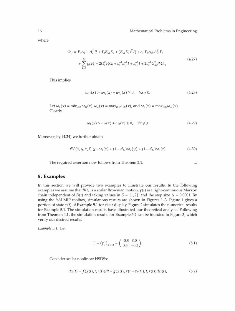
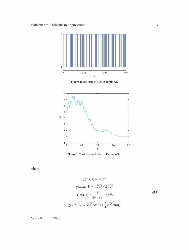
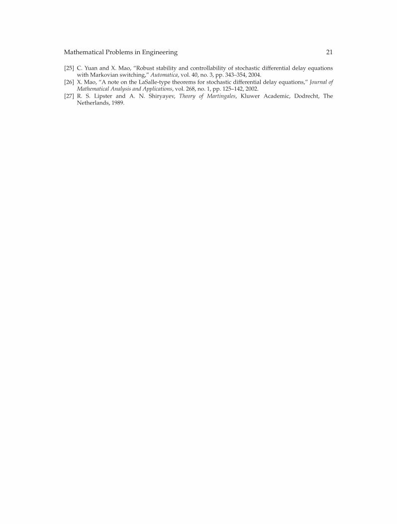
In this section we will provide two examples to illustrate our results. In the followingexamples we assume that B(t) is a scalar Brownian motion, γ(t) is a right-continuous Markovchain independent of B(t) and taking values in S = {1, 2}, and the step size Δ = 0.0001. Byusing the YALMIP toolbox, simulations results are shown in Figures 1–3. Figure 1 gives aportion of state γ(t) of Example 5.1 for clear display. Figure 2 simulates the numerical resultsfor Example 5.1. The simulation results have illustrated our theoretical analysis. Followingfrom Theorem 4.1, the simulation results for Example 5.2 can be founded in Figure 3, whichverify our desired results.

Example 5.1. Let

Γ =(γij)2 × 2 =

(−0.8 0.80.3 −0.3

). (5.1)

Consider scalar nonlinear HSDSs:

dx(t) = f(x(t), t, r(t))dt + g(x(t), x(t − τ2(t)), t, r(t))dB(t), (5.2)


2

1

0 0.01 0.02 0.03

t

Figure 1: The state γ(t) of Example 5.1.

t

7

6

5

4

3

2

1

0

−10 0.2 0.4 0.6 0.8

X(t)

Figure 2: The state evolution of Example 5.1.

where

f(x, t, 1) = −6 5√x,

g(x, z, t, 1) = − 5√x3 + 2 5

√z3,

f(x, t, 2) =3

2 3√1 + t

− 4 5√x,

g(x, z, t, 2) =5√x3 cos(t) +

54

5√z3 sin(t),

(5.3)

τ2(t) = 0.3 + 0.3 sin(t).


The controlled statesThe uncontrolled states

t

X(t)

1.2

1

0.8

0.6

0.4

0.2

0

−0.20 0.2 0.4 0.6 0.8 1

Figure 3: The state evolution of Example 5.2.

To examine the stability of system (5.2), we consider a Lyapunov function candidateV : R × S → R+ as V (x, i) = x2 for i = 1, 2. Then we have

LV (x, z, t, 1) ≤ −10x6/5 + 4z6/5,

LV (x, z, t, 2) ≤ 3x3√1 + t

− 6x6/5 +258z6/5.

(5.4)

By the elementary inequality αcβ1−c ≤ cα + (1 − c)β for all α ≥ 0, β ≥ 0, and 0 ≤ c ≤ 1,we see that inequality

3x3√1 + t

=(65κx6/5

)6/5(

6(κ

5

)−5(1 + t)−2

)1/6

≤ κx6/5 +κ1

(1 + t)2(5.5)

holds for any κ > 0, where κ1 = (κ/5)−5.From inequalities (5.4)–(5.5), we have

LV (x, z, t, i) ≤ κ1

(1 + t)2− (6 − κ)x6/5 + 4z6/5, (5.6)

for all t ≥ 0 and i ∈ S. By τ2(t) = 0.3 + 0.3 sin(t), it is easy to see that dτ2(t) < 1/3; then, wechoose constant κ such that 0 < κ < (2 − 6dτ2)/(1 − dτ2), and hence conditions of Theorem 3.1are satisfied.


Example 5.2. Let

Γ =(γij)2 × 2 =

(−0.6 0.60.5 −0.5

). (5.7)

Consider scalar nonlinear closed-loop HSDSs:

dx(t) =[f(x(t), x(t − τ1(t)), t, r(t)) + B(r(t))K(r(t))x(t)

]dt

+ g(x(t), x(t − τ2(t)), t, r(t))dB(t)(5.8)

with

f(x, y, t, 1

)= x +

12y +

2x3

(|x| + 1)2+ y sin(t),

g(x, z, t, 1) = x cos(t) +z3

(|z| + 1)2,

(5.9)

f(x, y, t, 2

)= −2x + y +

x3

(|x| + 2)2+

y3

(|y| + 1)2 ,

g(x, z, t, 2) = 2x sin(t) +x3

2(|x| + 1)2+

z3

(|z| + 2)2,

(5.10)

τ1(t) = 0.1 + 0.1 sin(t), τ2(t) = 0.2 + 0.2 sin(2t), B1 = 2, B2 = −3,A1 = 1,A2 = 2, Ad1 = 1/2,Ad2 = 1, F11 = 8, F12 = G11 = 2, G12 = F21 = F22 = 2, G21 = 1/2, G22 = 2.

By Theorem 4.1 we can find the feasible solution K1 = −3, K2 = 2 for the a.s. stability.

6. Conclusions

In this paper, we have investigated the a.s. stability analysis and stabilization synthesisproblems for nonlinear HSDSs. Some sufficient conditions are given to guarantee theresulting systems to be a.s. stable. Under these conditions, a.s. stabilization problem for aclass of nonlinear HSDSs is solved in terms of the solutions to a set of LMIs. Finally, theresults of this paper have been demonstrated by two numerical simulation examples.

Acknowledgment

This work is supported in part by the National Natural Science Foundation of P.R. China (no.60974030).

References

[1] J. Hu, Z. Wang, H. Gao, and L. K. Stergioulas, “Robust sliding mode control for discrete stochasticsystems with mixed time delays, randomly occurring uncertainties, and randomly occurringnonlinearities,” IEEE Transactions on Industrial Electronics, vol. 59, no. 7, pp. 3008–3015, 2012.


[2] L. Hu and X. Mao, “Almost sure exponential stabilisation of stochastic systems by state-feedbackcontrol,” Automatica, vol. 44, no. 2, pp. 465–471, 2008.

[3] X. Li and C. E. De Souza, “Criteria for robust stability and stabilization of uncertain linear systemswith state delay,” Automatica, vol. 33, no. 9, pp. 1657–1662, 1997.

[4] X. Li and C. E. De Souza, “Delay-dependent robust stability and stabilization of uncertain linear delaysystems: a linear matrix inequality approach,” IEEE Transactions on Automatic Control, vol. 42, no. 8,pp. 1144–1148, 1997.

[5] S. Ma, Z. Cheng, and C. Zhang, “Delay-dependent robust stability and stabilisation for uncertaindiscrete singular systems with time-varying delays,” Control Theory & Applications, vol. 1, no. 4, pp.1086–1095, 2007.

[6] B. Shen, Z. Wang, Y. S. Hung, and G. Chesi, “Distributed H∞ filtering for polynomial nonlinearstochastic systems in sensor networks,” IEEE Transactions on Industrial Electronics, vol. 58, no. 5, pp.1971–1979, 2011.

[7] D. Yue andQ. L. Han, “Delay-dependent exponential stability of stochastic systemswith time-varyingdelay, nonlinearity, and Markovian switching,” IEEE Transactions on Automatic Control, vol. 50, no. 2,pp. 217–222, 2005.

[8] L. Liu, Y. Shen, and F. Jiang, “The almost sure asymptotic stability and th moment asymptotic stabilityof nonlinear stochastic differential systems with polynomial growth,” IEEE Transactions on AutomaticControl, vol. 56, no. 8, pp. 1985–1990, 2011.

[9] G. Wei, Z. Wang, H. Shu, and J. Fang, “Robust H∞ control of stochastic time-delay jumping systemswith nonlinear disturbances,” Optimal Control Applications and Methods, vol. 27, no. 5, pp. 255–271,2006.

[10] G.Wei, Z.Wang, andH. Shu, “Nonlinear H∞ control of stochastic time-delay systemswithMarkovianswitching,” Chaos, Solitons and Fractals, vol. 35, no. 3, pp. 442–451, 2008.

[11] X. Mao, “Stochastic versions of the LaSalle theorem,” Journal of Differential Equations, vol. 153, no. 1,pp. 175–195, 1999.

[12] X. Mao, Y. Shen, and C. Yuan, “Almost surely asymptotic stability of neutral stochastic differentialdelay equations with Markovian switching,” Stochastic Processes and their Applications, vol. 118, no. 8,pp. 1385–1406, 2008.

[13] B. Bercu, F. Dufour, and G. G. Yin, “Almost sure stabilization for feedback controls of regime-switching linear systems with a hidden Markov Chain,” IEEE Transactions on Automatic Control, vol.54, no. 9, pp. 2114–2125, 2009.

[14] Z. Lin, Y. Lin, andW. Zhang, “H∞ filtering for non-linear stochasticMarkovian jump systems,”ControlTheory & Applications, vol. 4, no. 12, pp. 2743–2756, 2010.

[15] L. Wu, D. W. C. Ho, and C. W. Li, “Stabilisation and performance synthesis for switched stochasticsystems,” Control Theory & Applications, vol. 4, no. 10, pp. 1877–1888, 2010.

[16] L. Wu, D. W. C. Ho, and C. W. Li, “Sliding mode control of switched hybrid systems with stochasticperturbation,” Systems and Control Letters, vol. 60, no. 8, pp. 531–539, 2011.

[17] J. Yao, F. Lin, and B. Liu, “H∞ control for stochastic stability and disturbance attenuation in a class ofnetworked hybrid systems,” Control Theory & Applications, vol. 5, no. 15, pp. 1698–1708, 2011.

[18] N. Zeng, Z. Wang, Y. Li, M. Du, and X. Liu, “a Hybrid EKF and switching PSO algorithm for jointstate and parameter estimation of lateral flow immunoassay models,” IEEE/ACM Transactions onComputational Biology and Bioinformatics, vol. 9, no. 2, pp. 321–329, 2012.

[19] X. Mao, “Stability of stochastic differential equations with Markovian switching,” Stochastic Processesand their Applications, vol. 79, no. 1, pp. 45–67, 1999.

[20] C. Yuan and J. Lygeros, “Stabilization of a class of stochastic differential equations with Markovianswitching,” Systems and Control Letters, vol. 54, no. 9, pp. 819–833, 2005.

[21] X. Mao, J. Lam, and L. Huang, “Stabilisation of hybrid stochastic differential equations by delayfeedback control,” Systems and Control Letters, vol. 57, no. 11, pp. 927–935, 2008.

[22] Z. Wang, H. Qiao, and K. J. Burnham, “On stabilization of bilinear uncertain time-delay stochasticsystems with Markovian jumping parameters,” IEEE Transactions on Automatic Control, vol. 47, no. 4,pp. 640–646, 2002.

[23] Z. Wang, Y. Liu, and X. Liu, “Exponential stabilization of a class of stochastic system with markovianjump parameters and mode-dependent mixed time-delays,” IEEE Transactions on Automatic Control,vol. 55, no. 7, pp. 1656–1662, 2010.

[24] L. Huang and X. Mao, “On almost sure stability of hybrid stochastic systems with mode-dependentinterval delays,” IEEE Transactions on Automatic Control, vol. 55, no. 8, pp. 1946–1952, 2010.


[25] C. Yuan and X. Mao, “Robust stability and controllability of stochastic differential delay equationswith Markovian switching,” Automatica, vol. 40, no. 3, pp. 343–354, 2004.

[26] X. Mao, “A note on the LaSalle-type theorems for stochastic differential delay equations,” Journal ofMathematical Analysis and Applications, vol. 268, no. 1, pp. 125–142, 2002.

[27] R. S. Lipster and A. N. Shiryayev, Theory of Martingales, Kluwer Academic, Dodrecht, TheNetherlands, 1989.

Submit your manuscripts athttp://www.hindawi.com

Hindawi Publishing Corporationhttp://www.hindawi.com Volume 2014

MathematicsJournal of


Mathematical Problems in Engineering

Hindawi Publishing Corporationhttp://www.hindawi.com

Differential EquationsInternational Journal of

Volume 2014

Applied MathematicsJournal of


Probability and StatisticsHindawi Publishing Corporationhttp://www.hindawi.com Volume 2014

Journal of


Mathematical PhysicsAdvances in

Complex AnalysisJournal of


OptimizationJournal of


CombinatoricsHindawi Publishing Corporationhttp://www.hindawi.com Volume 2014

International Journal of


Operations ResearchAdvances in

Journal of


Function Spaces

Abstract and Applied AnalysisHindawi Publishing Corporationhttp://www.hindawi.com Volume 2014

International Journal of Mathematics and Mathematical Sciences


The Scientific World JournalHindawi Publishing Corporation http://www.hindawi.com Volume 2014


Algebra

Discrete Dynamics in Nature and Society



Decision SciencesAdvances in

Discrete MathematicsJournal of

Hindawi Publishing Corporationhttp://www.hindawi.com

Volume 2014 Hindawi Publishing Corporationhttp://www.hindawi.com Volume 2014

Stochastic AnalysisInternational Journal of

Almost Sure Stability and Stabilization for Hybrid ... · PDF fileHua Yang,1,2 Huisheng Shu,3...

Documents

Transcript of Almost Sure Stability and Stabilization for Hybrid ... · PDF fileHua Yang,1,2 Huisheng Shu,3...