Loughborough UniversityInstitutional Repository

Allocation of scarce waterresources using deficitirrigation in rotational

systems

This item was submitted to Loughborough University's Institutional Repositoryby the/an author.

Citation: GORANTIWAR, S.D. and SMOUT, I.K. 2003. Allocation of scarcewater resources using deficit irrigation in rotational systems. Journal of Irriga-tion and Drainage Engineering, 129 (3), pp. 155-163 [DOI 10.1061/(ASCE)0733-9437(2003)129:3(155)]

Additional Information:

• This journal article was published in the journal, Journal of Irrigationand Drainage Engineering [ c© ASCE]. The definitive version is availableat: http://cedb.asce.org

Metadata Record: https://dspace.lboro.ac.uk/2134/3607

Publisher: c© American Society of Civil Engineers (ASCE)

Please cite the published version.

This item was submitted to Loughborough’s Institutional Repository by the author and is made available under the following Creative Commons Licence

conditions.

For the full text of this licence, please go to: http://creativecommons.org/licenses/by-nc-nd/2.5/

1

ALLOCATION OF SCARCE WATER RESOURCES USING DEFICIT

IRRIGATION IN ROTATIONAL SYSTEMS

S.D.Gorantiwar1 and I.K.Smout2

ABSTRACT: On irrigation schemes with rotational irrigation systems in semiarid tropics,

the existing rules for water allocation are based on applying a fixed depth of water with every

irrigation irrespective of the crops, their growth stages and soils on which these crops are

grown. However when water resources are scarce, it is necessary to allocate water optimally

to different crops grown in the irrigation scheme taking account of different soils in the

command area. Allocating water optimally may lead to applying less water to crops than is

needed to obtain the maximum yield. In this paper, a three stage approach is proposed for

allocating water from a reservoir optimally based on a deficit irrigation approach, using a

simulation-optimization model. The allocation results with a deficit irrigation approach are

compared for a single crop (wheat) in an irrigation scheme in India, firstly with full irrigation

(irrigation to fill the root zone to field capacity) and secondly with the existing rule. The full

irrigation with a small irrigation interval was equivalent to adequate irrigation (no stress to

the crop). It is found that practising deficit irrigation enables the irrigated area and the total

crop production in the irrigation scheme used for the case study to be increased by about 30-

45% and 20-40%, respectively over the existing rule and by 50% and 45%, respectively over

the adequate irrigation. Allocation of resources also varied with soil types.

1 Academic Visitor, Water, Engineering and Development Centre, Loughborough University, Loughborough, Leics., LE11 3TU, UK 2 Director, Water, Engineering and Development Centre, Loughborough University, Loughborough, Leics., LE11 3TU, UK

2

Keywords. Soil water balance, Adequate irrigation, Deficit irrigation, Optimum land and

water allocation

INTRODUCTION

In irrigation schemes under a rotational water supply in the semi-arid tropics, normally

the fixed depth of water is applied with every irrigation, scheduled at a fixed interval

(existing rule), for ease of operation of the irrigation schemes. However with limited water

available for irrigation in those schemes, as indicated by an average irrigation intensity of 30

to 40% (Shanan, 1992), it is now obvious that irrigation water needs to be allocated

optimally by considering varied crops, their growth stages, different soils existing in the

irrigation schemes and efficiencies at different stages of movement of water from the

reservoir to the root zone.

Numerous techniques have been developed for optimal allocation of water resources,

based on optimization models. These techniques broadly fall into two categories. In the first

category, the water is allocated to different crops according to their water requirement for

producing maximum yield per unit area, and hence the area to be irrigated under different

crops is pre-determined (Afshar and Marino, 1989; Mayya and Prasad, 1989; Paudyal and

Gupta, 1990; Thandaveswara, 1992; Shyam et al., 1994 and Onta et al., 1995). However in

water limiting conditions, allocating less water than the maximum water requirement may

produce more production than allocating water equivalent to the maximum water

requirement.

In the second category, the water allocation considers several alternative levels of

water applied (and in some cases, alternative intraseasonal distributions) and the

corresponding yield over the entire season, either by specifying the area to be irrigated by

3

each crop (Dudley et al., 1971; Schmidt and Plate, 1980; Bras and Cordova, 1981; Rhenals

and Bras, 1981; Loftis and Houghtalen, 1987; Rao et al., 1990; Vedula and Mujumdar, 1992;

Akhand et al., 1995; Wardlaw and Barnes, 1999 and Paul et al., 2000) or by deciding the

optimal areas to be irrigated under different crops (Matanga and Marino, 1979; Sudar et al.,

1981; Yaron and Dinar, 1982; Rao et al., 1986; Sritharan et al., 1988; Bernardo et al., 1988;

Martin et al., 1989; Shyam et al., 1994 and Onta et al., 1995). The different combinations of

water applied and yield which are considered in these studies are mostly based on developing

a seasonal water production function for each crop. In these cases, allocation is based on the

optimum intraseasonal distribution of seasonal depth of water by a dynamic programming

approach and hence by considering the deficit irrigation. However in the further optimization

process (either optimum allocation of water or both area and water), the deficit itself is not

distributed optimally over both different intraseasonal periods and area.

At a scheme level, the problem also needs to be solved differently due to variation in

soil types, different irrigation efficiencies at different application levels, and sensitivity of

crops to water application during different crop growth stages. The most appropriate

approach in a multicrop and water limiting situation is to use several sets of water application

depths based on combination of full and deficit irrigation over different irrigation or

intraseasonal periods, and the corresponding crop yields. This approach is adopted in this

paper to include deficit irrigation in the optimization process. The set of irrigation depths per

irrigation application and crop yield or net benefits per unit area is termed an ‘irrigation

program’ in this paper.

In the present paper, several irrigation programs are generated for each crop-soil

combination, by using a soil water balance crop growth simulation model and including

deficit irrigation and irrigation efficiencies at different stages. Deficit irrigation is included

by considering irrigation depths to bring the soil to field capacity i.e. full irrigation and to

4

below field capacity i.e. partial irrigation. These programs are then incorporated in a resource

optimization model to allocate land and water optimally for irrigation schemes, where

shortages of water prevent adequate irrigation of the whole irrigable command area of the

irrigation scheme. The allocation of land and water resources obtained with deficit irrigation

using the model developed in this study is compared with the existing rule of applying a

fixed depth of irrigation water and with full irrigation, by using a case study for a single crop

(wheat) grown on an irrigation scheme in a semi-arid region in western India. This

demonstrates the influence of soil type and irrigation interval on allocation of the resources

by existing and proposed rules. In these irrigation systems, the irrigation interval is assumed

to be pre-determined and uniform for all crop and soil combinations.

The terms full irrigation and partial irrigation in the context of deficit irrigation are

described in the next section.

DEFICIT IRRIGATION

Deficit irrigation has been defined as deliberate underirrigation of a crop (English and

Nuss, 1982 and English, 1990), purposefully planned underirrigation (Keller et al., 1992) or

deliberate stressing of crops (Hargreaves and Samani, 1984) to influence the yield or profit.

Trimmer (1990) defined deficit irrigation similarly as the practice of scientifically

underirrigating crops to reduce yield in a controlled way. The purpose of the underirrigation

was to spread available water over a large area, thereby increasing the total production from

the irrigation scheme or reducing the total use of water or energy per unit area irrigated. All

these researchers explained the effect of deficit irrigation in reducing the seasonal depth of

irrigation. The present paper is concerned with optimizing the depth of irrigation per

application in a water limiting condition and a multicrop and soil situation to obtain the

5

maximum output (in the form of crop production or net benefits) from the irrigation scheme,

so the terminology is elaborated further.

The inadequacy of available water supplies to irrigate the entire arable land presents

two alternatives to the irrigator:

(1) Irrigate a limited area by applying water equivalent to the maximum crop water

requirement so that the crop is not subjected to water stress, and maximum yields per hectare

of irrigated area are obtained. This is called "adequate irrigation".

(2) Irrigate more land than can be irrigated with option (1) by applying less water than the

maximum crop water requirement, causing stress to the crop and resulting in reduced yield

per hectare but with more land under irrigation. This is called "deficit irrigation".

Adequate irrigation gives the maximum crop yield per unit of land irrigated. Deficit

irrigation could be followed to give the maximum crop yield per unit of water utilized and/or

maximum total production (and/or maximum net benefits) over the irrigation scheme. The

practices of adequate and deficit irrigation can be followed by applying full or partial

irrigation at each irrigation depending on the interval between two irrigations. For a small

irrigation interval, even with partial irrigation, stress may not occur, and for a large irrigation

interval, stress may also be caused with full irrigation. Thus the adequate irrigation is:

applying full or partial irrigation at each irrigation with the interval between irrigations

adjusted to maintain maximum crop evapotranspiration (ET) and thus not to cause any stress,

so that maximum crop yields are obtained. Deficit irrigation is: applying full or partial

irrigation at each irrigation but with the interval between them causing actual crop ET to

drop below maximum crop ET, which results in stress and subsequent reduction in crop yield

and in the process using less water than for adequate irrigation.

With finite supplies of water, many researchers found that applying less water than

required for maximum yield, is beneficial in terms of profit (English and Nuss,1982; Reddy

6

and Clyma,1983; Hargreaves and Samani,1984; English,1990; Trimmer,1990 and Keller et

al., 1992). In deficit irrigation, the crop is subjected to water stress resulting in a reduction of

crop yield which depends on the timing and amount of deficit. The deficit can be obtained by

following three approaches.

Approach-1 : Prolonging the interval between two irrigation applications beyond the

irrigation interval which would not cause any stress to the crop, if the root zone was filled up

to field capacity, and applying water to bring soil moisture in the root zone to field capacity.

The crop is subjected to stress at the end of each irrigation period (the case of full irrigation

with a large irrigation interval).

Approach-2 : Applying less water than the amount required to bring the soil moisture in the

root zone to field capacity, with an irrigation interval which would not cause any stress if the

root zone was filled up to field capacity (the case of partial irrigation with a small irrigation

interval).

Approach-3 : Combination of (1) and (2) i.e. by prolonging the irrigation interval beyond the

one which does not cause any stress when the root zone is filled to its field capacity and

applying less water than required to bring the soil root zone to field capacity (the case of

partial irrigation with a large irrigation interval).

Fig. 1 shows the soil water status in the root zone in response to irrigation compared

to soil water at field capacity and wilting point and readily available soil water and illustrates

all these approaches schematically. The readily available soil moisture is obtained from

allowable depletion which is a function of maximum crop evapotranspiration (Doorenbos

and Kassam, 1986). In the present study full and partial irrigations are applied for different

irrigation intervals and therefore Approach-2 is practised for smaller irrigation intervals and

7

Approach-1 and Approach-3 are practised for large irrigation intervals. However as the

allocation model is developed for irrigation schemes with large command areas and

rotational irrigation systems, the irrigation interval is kept the same for all crops in the season

and all soils in the command. Application of less water is indicated by a term 'deficit ratio'

which is prescribed for each irrigation application and is the ratio of the amount of water

applied to the root zone to the amount of water required to fill the root zone to field capacity.

Each combination of crop and soil is referred to as a ‘unit’.

RESOURCE ALLOCATION MODEL WITH DEFICIT IRRIGATION

A three stage resource allocation model with deficit irrigation, Area and Water

Allocation Model (AWAM), which uses a simulation optimization technique was developed.

The three stages are

(1) Generation of alternative irrigation programs based on deficit irrigation for each unit

(2) Selection of optimal irrigation programs

(3) Allocation of the resources (land and water)

The model is described in detail by Gorantiwar (1995). In this paper the important

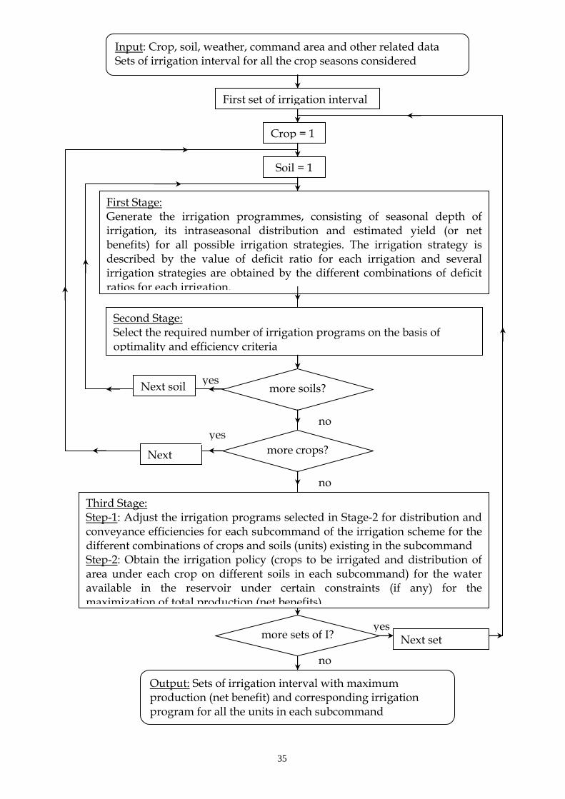
features of the model are presented. The flow chart of model, AWAM, is presented in Fig. 2.

Stage 1: Generation of Alternative Irrigation Programs

In the present study, the term "irrigation strategy" is used to represent, for a particular

irrigation interval, the values of deficit ratios associated with each irrigation application.

There can be several irrigation strategies and these are obtained by different combinations of

deficit ratio for each irrigation application. In this stage the irrigation programs are generated

for different irrigation strategies for the unit by formulating Soil WAter Balance - Crop Yield

8

Benefit (SWAB-CRYB) simulation model. This model has some default procedures or

models for simulation of many parameters (Retta and Hanks, 1980; Doorenbos and Pruitt,

1984; Doorenbos and Kassam, 1986; Walker and Skogerboe, 1987; Bos and Nugteren, 1990

and Smith, 1991) but also allows the user to stipulate other procedures or models or make

direct input of certain parameters. The model SWAB-CRYB is formulated to make it

applicable to major field crops grown in the command area of an irrigation scheme. It uses

the data which are generally available at the irrigation scheme, if any, and general data

documented by FAO (Doorenbos and Pruitt, 1984 and Doorenbos and Kassam, 1986), if

local data are not available. The soil water balance part of this model represents the system

more descriptively than used in most allocation studies. The model SWAB-CRYB involves

various inflow and outflow processes, a soil water balance equation and crop growth model.

The details of the SWAB-CRYB model are described by Gorantiwar (1995).

Stage 2: Selection of Optimal Irrigation Programs

At this stage optimal irrigation programs are selected from all the irrigation programs

generated at stage-1 for each irrigation strategy. A strategy consists of a series of irrigations,

each of which may have a different deficit ratio.

Total irrigation programs : If 'Δa' is the increment chosen between deficit ratios, the number

of possible deficit ratios (na) is computed by equation (1).

( ){ } 1a/aminamaxna +Δ−= (1)

where amax= maximum value of deficit ratio (usually one) and amin = minimum value of

deficit ratio (usually zero). The total number of irrigation strategies considered (P) is

computed by equation (2).

9

1)(IcnaP −= if first irrigation is to fill entire root zone

IcnaP = otherwise (2)

where Ic = total number of irrigation applications (excluding presowing irrigation). The

presowing irrigation, if needed, is given to fill the soil zone to field capacity. Thus there can

be ‘P’ total irrigation programs (corresponding to P irrigation strategies). The optimal

irrigation programs (OIPs) are selected from these total irrigation programs. The OIP is the

irrigation program with an output more than the output from other irrigation programs but

with a seasonal irrigation depth the same or less than the seasonal irrigation depth of other

irrigation programs. It is obvious that in a water limiting condition and multicrop and soil

situation, one or more OIP(s) can appear in the solution. If the number of irrigation programs

to be transferred to the third stage is to be limited due to the restriction on the number of

variables that can be considered in the optimization model of stage-3, only those OIPs are

selected which give a higher marginal increase in yield (net benefits) with increase in water

applied than the other OIPs. These programs are referred to as selected OIPs (SOIPs). In

other words these are the most economically efficient optimal irrigation programs. There

may be a small possibility of losing optimality by restricting the number of OIPs but it can be

risked for computational feasibility. This has been confirmed by comparing the results when

all OIPs are considered as SOIPs and when few OIPs are selected as SOIPs (Gorantiwar,

1995). SOIPs appearing in the solution of the optimization model of third stage (allocation of

the resources) are termed final irrigation programs.

Stage 3: Allocation of the Resources

10

In this stage, the land and water resources are allocated optimally to different crops

grown on various soils in different locations in the command. This is done in two steps

(modification of SOIPs and optimization). It is assumed that the entire command can be

divided into several subcommands, each characterized by its own distribution efficiency (the

efficiency of the water distribution canals supplying water from the conveyance network to

individual fields) and the distance from the main feeder canal (or conveyance losses from the

main feeder canal to the subcommand). Soils within the subcommand may vary and different

crops can be grown in the subcommand. In first step, the SOIPs generated for different units

are modified for the units in each subcommand by giving consideration to distribution and

conveyance efficiencies and in second step land and water resources are optimally allocated

with specified objective and constraints.

Modification of SOIPs : Less than half of the water diverted from the headworks usually

reaches the crop root zone. The water lost in this process at different places is represented by

different irrigation efficiencies and hence the proper consideration of these efficiencies in the

allocation is very important rather than assuming by a single value (generally project

efficiency). The SOIPs generated in the second stage consider the field application efficiency

which may be different for different units and is a function of soil, crop, irrigation method

and depth of irrigation. The other efficiencies (distribution and conveyance) which depend

on characteristics of subcommand and its location in the command cannot be considered

while generating SOIPs. Therefore they are modified in this third stage for variation of

efficiencies with location and time. The irrigation depth of each irrigation application is

adjusted for distribution and conveyance efficiencies and the total irrigation delivery (D) is

obtained. The value of these efficiencies (which may vary with subcommand and irrigation)

11

can be given as input to the model or decided in the model by using the values proposed by

ILRI (Bos and Nugteren, 1990).

Optimization : The primary objective of this step is to allocate available land and water

resources to different activities (each unit of each subcommand is a separate activity) for

obtaining maximum net benefits or production or for irrigating maximum area when

subjected to certain restrictions. The linear programming approach can handle this situation

and is adopted to obtain the solution. The part of the optimization model which is used for

the case study is described in this section. The details of the optimization model are

described by Gorantiwar (1995).

(1) OBJECTIVE FUNCTION

The objective function is the maximization of the total net benefits which is the

common objective for many irrigation schemes. Alternatively, if it is decided to

maximize the food production instead of obtaining maximum net benefits, the

objective function is the maximization of total production. However this can be

adopted only when a single crop is grown in the irrigation scheme.

(2) CONSTRAINTS

The following constraints are included in the model.

(a) Area Constraints : Area to be irrigated for each soil type under each subcommand should

be less than maximum available area under this soil type in the subcommand.

(b) Crop Area Related Constraints : In a multicrop situation it is possible that only one crop

appears in the solution for maximizing the objective function. However the areas to be

12

irrigated under different crops may need to be adjusted according to the different

requirements in the irrigation scheme. These may include requirements to follow a certain

crop mix, to satisfy the food requirements of the inhabitants in the command area and to

restrict the area to be irrigated under different crops in a certain range. The constraints to

restrict the area to be irrigated for different crops are included in the model by specifying the

range of area to be irrigated for all or certain crops.

(c) Water Related Constraints :

Intraseasonal water supply : The total quantity of water applied to various activities in any

intraseasonal period (irrigation period) should not be greater than the water storage available

during the irrigation period under consideration.

Storage : Storage of water in the reservoir during any of the intraseasonal periods should not

be less than the minimum allowable level (dead storage capacity) or more than the maximum

level (reservoir capacity)

Canal capacity : Water to be released in any of the irrigation periods should not exceed the

carrying capacity of the main canal. The water to be released to each subcommand during

any of the irrigation periods should not exceed the capacity of the secondary/tertiary canal or

outlet corresponding to the subcommand.

(d) Non-negativity constraints : The values of different activities should be greater than or

equal to zero.

RESULTS

13

A case study is presented for the irrigation scheme in the semi-arid region of the

western state of India to compare the allocation of the resources with three different

allocation rules - the existing rule, full irrigation and the deficit irrigation approach- and to

discuss the utility of the proposed method. The entire command area of the scheme was

considered as the subcommand with a single crop (wheat), to limit the complexities in the

discussion of the influence of different rules of allocation, irrigation interval and soil type on

the allocation. These complexities may arise due to sensitivity of prices for different crops

and variation of irrigation efficiencies of each subcommand. The culturable command area

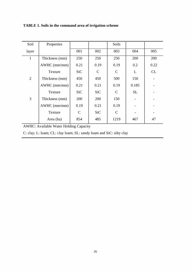
(CCA) of the project is 3072 ha and consists of five different soil types. These are described

in Table 1. The soil type 005 was not considered suitable for the cultivation of wheat. The

crop period of wheat grown in the region is 120 days.

The model SWAB-CRYB of stage-1 was tested by using the field data generated at

the College of Agriculture, Pune (India), 75 Km away from the irrigation scheme (Jadhav,

1991). The linear root growth model (Fereres et al., 1981) was assumed to simulate the daily

root zone depth over the crop season. The rate of moisture extraction through transpiration

was considered to vary over the depth of the root zone and for that, the root zone on any day

was divided into four layers, each having the same thickness and with extraction rates of 40,

30, 20 and 10 % of total actual transpiration, beginning from the top layer. The crop

coefficients were estimated by using the polynomial function (equation 3) developed with

lysimetric data of three years for wheat (Suryawanshi et al., 1990) at Mahatma Phule

Agricultural University, Rahuri (India), 150 Km away from the irrigation project.

432

t Tt2.67

Tt4.84

Tt1.44

Tt3.430.28Kc ⎟

⎠⎞

⎜⎝⎛+⎟

⎠⎞

⎜⎝⎛−⎟

⎠⎞

⎜⎝⎛−⎟

⎠⎞

⎜⎝⎛+= (3)

14

where Kc = crop coefficient value, t = number of days since planting and T is crop period in

days

The maximum grain yield that can be obtained was 4000 kg/ha. The yield response

factors computed from experimental data (Jadhav, 1991) were used (0.187, 1.009, 0.417,

0.329, 0.235 and 0.017 for crown root initiation, tillering, jointing, flowering, milking and

physiological maturity stages, respectively) for estimating actual grain yield by additive type

of crop growth model based on evapotranspiration (Stewart and Hagan, 1973). The

climatological data of the experimental site for the year 1989-90 were used. The reference

crop ET was computed by a modified Penman method (Doorenbos and Pruitt, 1984 and

Smith, 1991). No rainfall was received in the crop period. The minimum and maximum

permissible irrigation depth values were assumed as 50 and 150 mm per irrigation,

respectively. The initial soil moisture contents of all soil layers were assumed at field

capacity as the crop season under consideration follows the rainy season. The field

application efficiency, distribution efficiency and conveyance efficiency were considered as

0.75, 0.8 and 0.9, respectively. The full supply and dead storage capacities of the reservoir

were 22.31 and 5.68 Mm3, respectively. The water to be kept aside for non irrigation

purposes and for irrigating other areas is 8.69 Mm3. The streamflow and other data

(evaporation and seepage losses) were used for the year 1989-90. The carrying capacity of

the main canal is 1.53 m3/s.

Deficit Irrigation

The interval for computing the deficit ratio was taken as 0.1 and the deficit ratio

ranged from 0 to 1. Deficit ratio equal to 0 indicates no irrigation and equal to 1 means

irrigation is applied to bring moisture in the root zone to field capacity. In fact an irrigation

15

strategy having zero deficit ratio for any irrigation indicates that the irrigation application is

skipped and the water delivery interval is prolonged. Thus in deficit irrigation, for a

particular value of irrigation interval, the actual water delivery interval may be a multiple of

the irrigation interval under consideration. However for other cases of irrigation (full

irrigation and irrigation by existing rule), the irrigation interval and the water delivery

interval are the same because water is applied at every turn.

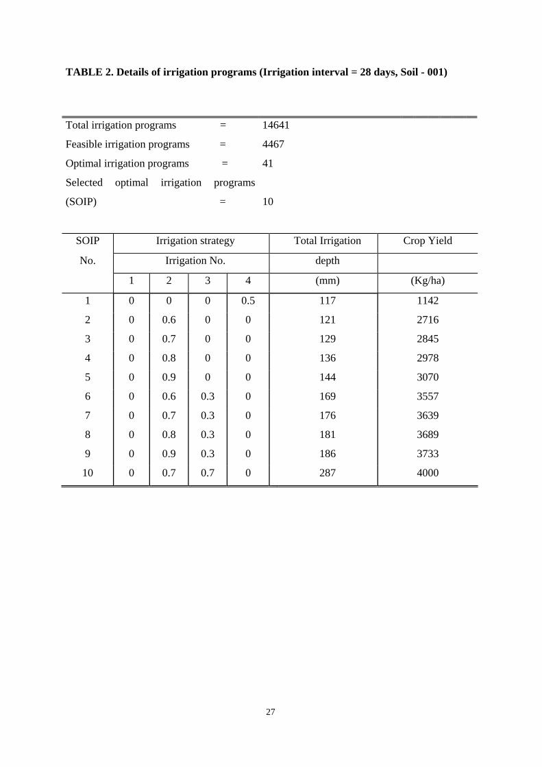
The model AWAM is run for the irrigation intervals of 14, 21, 28 and 35 days. The

details of ten SOIPs are presented in Table 2 for Soil - 001 and irrigation interval of 28 days.

The results of the land and water allocation are presented in Table 3. It is seen from Table 3

that with deficit irrigation the allocation results (areas and production) are similar for all

irrigation intervals except for 35 days. The total production is reduced when the irrigation

interval is increased to 35 days. The similar results for irrigation intervals of 14, 21 and 28

days are due to the flexibility in applying the depth of irrigation for different irrigations.

Irrigation strategies corresponding to the irrigation programs which appeared in the solution

show that the values of deficit ratios are adjusted, or irrigations are skipped, to develop an

optimum solution for these intervals. This is evident by comparing the irrigation strategies of

soil-002 for intervals of 14 and 28 days. Irrigation water is allocated for the second and

fourth irrigations when I=14 days and to the first and second when I=28 days. The slightly

higher production with I=14 days is due to greater flexibility in distributing the deficits over

more irrigation applications. The reduction in yield due to deficit caused by prolonging the

interval up to 35 days is considerable, and therefore the total production is also less. Among

the other irrigation intervals, though an interval of 14 days produces slightly more production

(about 5%), an interval of 28 days is preferable in view of possible saving in the cost of

applying irrigation. However in a multicrop situation, the irrigation strategy may change due

to the different sowing dates and the sensitivity of crop yield to the water availability in

16

different crop growth stages. It is also seen in Table 3 that two different irrigation strategies

for the same soil appeared in the solution (Soil - 001 for I=35 days and Soil - 003 for I=21

and 28 days). In these cases, all the area could be brought under irrigation due to deficit

irrigation and after allocating all the area to the most efficient irrigation strategy, there was

still some water left to be allocated. This remaining water was allocated to some area by

replacing the most efficient irrigation strategy by the next most efficient irrigation strategy

which gave a higher total yield than the most efficient irrigation strategy.

Full Irrigation

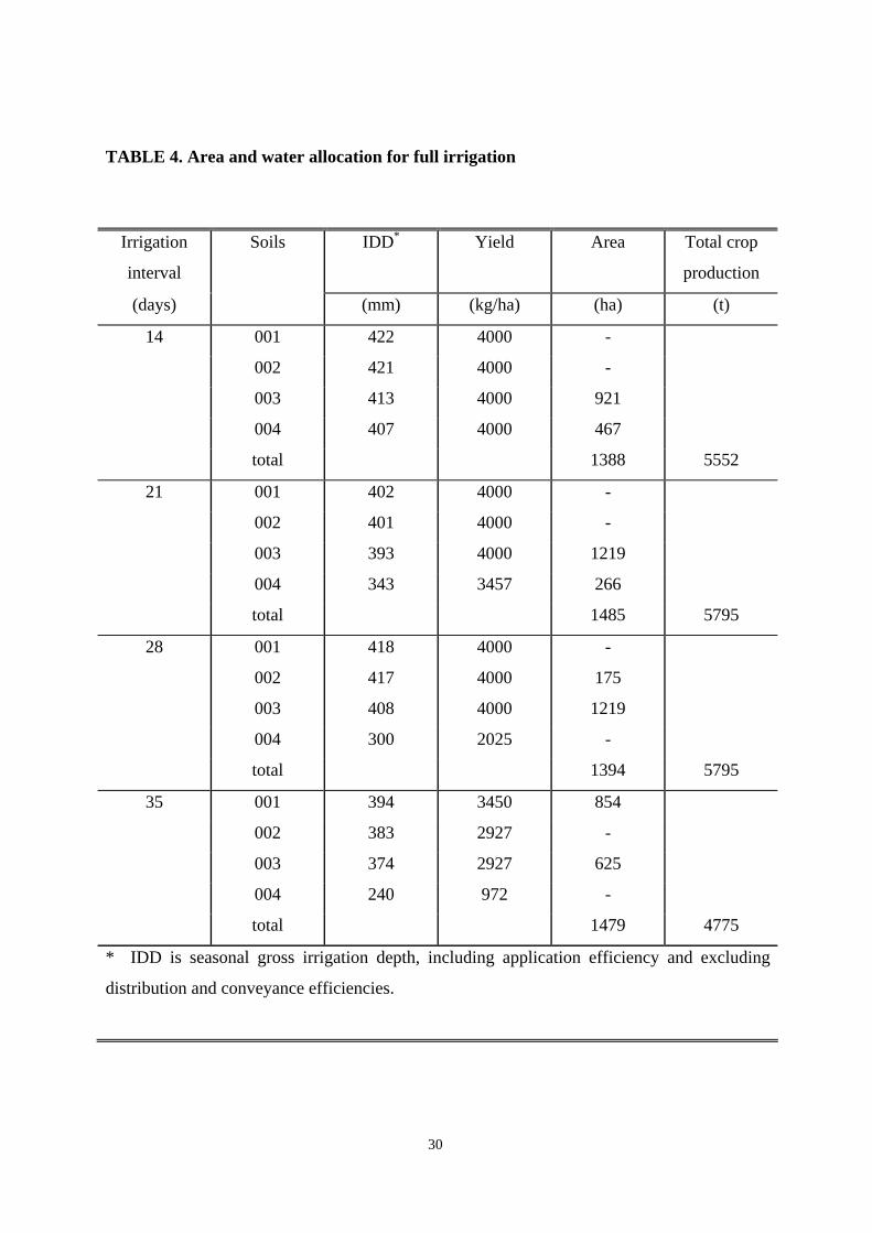
The allocation results for full irrigation are obtained when the irrigation is applied to

fill the root zone to field capacity, as presented in Table 4. It is observed from the results that

when full irrigation is given, the deficit did not occur up to an irrigation interval of 28 days

for the soils appearing in the solution, and when the irrigation is prolonged further (I=35

days), deficit occurred which is reflected in the reduction in yield. The higher total

production for I=14, 21 and 28 days than I=35 days indicates that the water saved due to

deficit caused by prolonging the irrigation interval did not produce enough to compensate for

the deficit. Irrigation intervals of 14, 21 and 28 days gave almost similar total production.

Though I=21 days gave slightly more production, I=28 days is preferred due to the lower

cost of waterings. Thus 28 days is the appropriate irrigation interval if the root zone is to be

filled to field capacity at each irrigation application and higher production per unit of water

consumed is needed.

The full irrigation with I = 14, 21 and 28 days represents the case of adequate

irrigation as the crop was not subjected to stress except for Soil 004 for which only I=14 days

represents the case of adequate irrigation (as evidenced by the yield values in Table 4). When

the results of adequate irrigation are compared with the deficit irrigation for I = 14, 21 and 28

17

days (Table 3), it is seen that the total production with deficit irrigation is almost twice the

total production obtained with adequate irrigation. This is achieved by bringing more area

under irrigation (almost two times more) with water saved due to deficit irrigation. It was

possible to extend the irrigation to the entire CCA with deficit irrigation if I = 21 or 28 days.

Thus in this case the practice of deficit irrigation is beneficial over the practice of adequate

irrigation, when compared for obtaining crop production.

As the full irrigation with I = 35 days caused the stress, it represents the case of

Approach-1 (Table 4). The full irrigation with I = 14, 21 and 28 days for Soil 001, Soil 002

and Soil 003 and full irrigation with I = 14 days for Soil 004 did not cause the stress.

Therefore partial irrigations for these irrigation intervals represent Approach-2 (Table 3). As

an irrigation interval of 35 days caused stress with full irrigation (Approach-1), the partial

irrigation for this irrigation interval represents the case of Approach-3 (Table 3). Approach-1

and Approach-3, in which the interval is prolonged beyond the one which does not cause

stress with full irrigation, give less production than Approach-2 where the irrigation interval

is not prolonged as in Approach-1 and Approach-3. This indicates that deficit irrigation by

prolonging the irrigation interval is not beneficial. Similarly comparing Approach-1 and

Approach-3 shows that Approach-3 resulted in higher production. This indicates that deficit

irrigation by applying water in depths less than required to fill the root zone to field capacity

(partial irrigation) is beneficial over full irrigation.

Existing Recommended Rule

The existing recommended rule for irrigation in the scheme is to deliver 70 mm of

water to the field or 52.5 mm to the root zone at each irrigation application. The results

obtained with this policy are presented in Table 5. An irrigation interval of 28 days gives

maximum total production. The existing recommended irrigation interval for the project is 21

18

days. But if only wheat is to be irrigated, an irrigation interval of 28 days is more appropriate

for this irrigation project. Irrigation intervals of 14 and 21 days do not cause any deficit and

give the potential yield, but need more water due to the greater number of irrigation

applications. Irrigation intervals of 14 and 21 days represent adequate irrigation. When the

irrigation interval is 28 days, the recommended 52.5 mm water is less than the depth required

to bring soil moisture to field capacity and as I = 28 days does not cause any stress with full

irrigation, it is equivalent to Approach-2 except for Soil 004. An irrigation interval of 35

days represents the case of Approach-3. With application of a fixed depth of irrigation also,

Approach-2 gives greater production than Approach-3. The total production amounts

obtained with different approaches for a fixed depth of water application are less than those

obtained with different approaches for deficit irrigation due to loss of water in deep

percolation when a fixed depth of water was applied for each irrigation.

When the total production amounts obtained with irrigation intervals of 21 and 28

days are compared for the existing recommended rule and the deficit irrigation approach

proposed in this paper, the deficit irrigation produces about 20-40% more total production by

irrigating about 30-45% more land. The deficit irrigation also gave 45% more total

production than full irrigation by irrigating about 50% more land. The deficit irrigation

approach suggested in this paper distributes the deficit optimally over all the irrigations (by

preparing irrigation programs for all possible irrigation strategies and including selected

optimal irrigation programs in the optimization process) and hence it is possible to reduce the

use of water per unit area. However in the full irrigation and existing rule approaches, at least

the minimum possible irrigation depth is applied at every application. Therefore there is a

possibility of excessive deep percolation losses when the depth of water application is low

(for example during initial crop growth stages). However in the deficit irrigation depth

approach, the irrigation can be skipped and hence it is possible to reduce deep percolation

19

losses. Therefore with the deficit irrigation approach higher crop production is obtained by

bringing more area under irrigation with the same amount of water, over existing rule of

applying fixed depth of irrigation and full irrigation. This would also bring major social

benefits by increasing the number of farmers receiving irrigation water.

Soils

Area and water allocation results (tables 3, 4 and 5) indicate that soil types influence

the allocation of the resources. When the allocation is based on the existing recommended

rule, the resources are allocated equally for a small irrigation interval, as the small irrigation

interval did not cause any stress and the rule was to apply the same depth of irrigation.

However as the irrigation interval is increased, the soils having lower water holding capacity

(WHC) experienced more stress as they cannot store water efficiently in the root zone at the

time of irrigation as compared to the soils having a higher WHC. Therefore the yields are

lower for these soils for the same depth of irrigation water applied and the resources are first

allocated to the soils having higher WHC. In deficit irrigation practice, the depth of irrigation

can be varied at each irrigation application and for each soil. Therefore the trend is to

distribute the available water optimally over all irrigation applications and soils to get

maximum production and as already discussed, practicing deficit irrigation leads towards the

maximization of production. The water saved through deficit irrigation of the soils having a

higher WHC could bring area from other soils under irrigation. If the full irrigation is

practiced, stress did not occur up to an irrigation interval of 28 days (except for soil 004), and

the soils with lower WHC (among the soils which did not experience stress) got allocation

first, as they needed less full depth of irrigation to give the maximum yield. However if the

irrigation interval is further increased, all the soils experienced stress and area was allocated

first to the soil which can keep the plant under no stress condition for a longer time (soils

20

with a higher WHC). Thus the allocation of the resources varies with the soils and irrigation

option, and therefore variation in soils needs to be considered in the optimization models.

SUMMARY AND CONCLUSION

The command area of a typical irrigation scheme with a rotational irrigation system

in the semiarid tropics may include several soil types on which different crops can be grown.

Where the availability of the water is limited compared to land, crops cannot be irrigated by

applying the required depth to obtain the potential yield over the whole area. Therefore the

available water needs to be allocated systematically. Under existing rules, the fixed depth of

water is applied with every irrigation irrespective of the crops, their growth stages and soils

on which these crops are grown in the command area of these irrigation schemes. However

when water resources are scarce, it is necessary to allocate water optimally to different crops

grown in the irrigation scheme taking account of different soils in the command area. Several

techniques have been developed to allocate land and water resources optimally by assuming

the allocation policy of one of them as known. However in the water limiting condition, as in

many irrigation schemes in semi-arid regions, the optimum allocation of these resources is

interdependent and so they need to be allocated together.

A three stage optimization simulation model which uses a deficit irrigation approach

is described in this paper. In the first stage several irrigation programs are generated for each

crop and soil type in the command. The field application efficiency is considered in this

stage, based on the parameters dependent on crop and soil. The second stage selects the few

most economically efficient irrigation programs. The third stage modifies the selected

irrigation programs by considering distribution and conveyance efficiencies at different

21

locations in the command area and allocates the resources optimally to different crops by

using these irrigation programs.

The model is applied to an irrigation scheme in a semi-arid region of India by

formulating a case study for a single crop (wheat) and the applicability of the model in

different situations is briefly discussed. The results are obtained for the water delivery

intervals of 14, 21, 28 and 35 days by a deficit irrigation approach. These are compared with

full irrigation (when water is delivered to fill the root zone to field capacity) and the existing

recommended rule (where water is applied in a fixed amount at every irrigation). The full

irrigation with I = 14, 21 and 28 days represent adequate irrigation (no yield reductions).

It was found in the case study that when the existing recommended rule is used, an

irrigation interval of 28 days is appropriate to obtain maximum production as against the

standard irrigation interval of 21 days. With deficit irrigation, intervals of 14, 21 and 28 days

gave similar results due to the different combinations of several depths of deficit irrigation.

However the water delivery interval of 28 days is proposed in view of the possible saving on

cost of applying irrigation water and operational ease. By practising the deficit irrigation

approach proposed in this paper, the total production and irrigated area could be increased by

20-40% and 30-45%, respectively over the existing recommended rule and by about 45% and

50%, respectively over full irrigation.

The model can consider the effect of various soils on the allocation and also the effect

of irrigation efficiencies which represent the major part of water consumed in the allocation

process, and can be applied to irrigation schemes growing several different crops.

APPENDIX. REFERENCES

22

Afshar, A. and Marino, M. A. (1989). “Optimization models for wastewater reuse in

irrigation ” J. Irrig. and Drain. Engrg., ASCE, 115(2), 185-202.

Akhand, N. A., Larson, D. L. and Slack, D. C. (1995). “Canal irrigation allocation planning

model.” Trans. ASAE, 38(2), 545-550.

Bernardo, D. J., Whittlesey, N. K., Saxton, K. E. and Bassett, D. L. (1988). “Irrigation

optimization under limited water supply.” Trans. ASAE 31, (3), 712-719.

Borg, H. and Grimes, D. W. (1986). “Depth developments of roots with time: An empirical

description.” Trans. ASAE, 29(1), 194-197.

Bos, M.G. and Nugteren, J. (1990). On Irrigation Efficiencies. International Institute for

Land Reclamation and Improvement, Wageningen, The Netherlands.

Bras, R. L. and Cordova, J. R. (1981). “Intraseasonal water allocation in deficit irrigation”.

Water Resour. Res., 17(4), 866-874.

Doorenbos, J. and Kassam, A. H. (1986). “Yield response to water.” Food and Agric. Org.

Irrig. And Drain. Paper 33, United Nations, Rome, Italy.

Doorenbos, J. and Pruitt, W. O. (1984). “Crop water requirements.” Food and Agric. Org.

Irrig. And Drain. Paper 24, United Nations, Rome, Italy.

Dudley, N. J., Howell, D. T. and Musgrave, W. F. (1971). “Optimal intra-seasonal irrigation

water allocation.” Water Resour. Res., 7(4), 770-788.

English, M. (1990). “Deficit irrigation I: Analytical framework.” J. Irrig. and Drain. Engrg.,

ASCE, 116(3), 399-412.

English, M. and Nuss, G. S. (1982). “Designing for deficit irrigation.” J. Irrig. and Drain.

Engrg., ASCE, 108(IR2), 91-106.

Fereres, E., Goldfien, R. E., Pruit, W. O., Henderson, D. W. and Hagan, R. M. (1981). “The

irrigation management program: A new approach to computer assisted irrigation

23

scheduling”. In Proc. Irrigation Scheduling for Water and Energy Conservation in the 80's,

ASAE, St. Joseph, Michigan ,USA:202-207.

Gorantiwar, S. D. (1995). “A model for planning and operation of heterogeneous irrigation

schemes in semi-arid regions under rotational water supply” A Ph. D. Thesis, Loughborough

University of Technology, Loughborough, Leicestershire, UK.

Hargreaves, G. H. and Samani, Z. A. (1984). “Economic considerations of deficit irrigation.”

J. Irrig. and Drain. Engrg., ASCE, 110(4), 343-358.

Keller, J., Sivanappan, R. K. and.Varadan, K. M. (1992). “Design logic for deficit drip

irrigation of coconut trees.” Irrigation and Drainage Systems, 6, 1-7.

Loftis, J. M. and Houghtalen, R. J. (1987). “Optimizing temporal water allocation by

irrigation ditch companies.) Trans. ASAE, 30(4), 1075-1082.

Martin, D., J. van Brocklin and Wilmes, G. (1989). “Operating rules for deficit irrigation

management.” Trans. ASAE, 32(4), 1207-1215.

Matanga, G. B. and Marino, M. A. (1979). “Irrigation planning 1. Cropping pattern.” Water

Resour. Res., 15(3), 672-678.

Mayya, S. G. and Prasad, R. (1989). “System analysis of tank irrigation: I. Crop staggering.”

J. Irrig. and Drain. Engrg., ASCE, 115(3), 384-405.

Onta, P. R., Loof, R. and Banskota, M. (1995). “Performance based irrigation planning under

water shortage.” Irrigation and Drainage Systems, 9, 143-162.

Paudyal, G. N. and Gupta, A. D. (1990). “Irrigation planning by multilevel optimization.” J.

Irrig. and Drain. Engrg., ASCE, 116(2), 273-291.

Paul, S., Panda, S.N. and Kumar, N. (2000). “Optimal irrigation allocation: A multilevel

approach.” J. Irrig. and Drain. Engrg., ASCE, 126(3), 149-156.

24

Rao, K. S. V. V. S., Reddi, T. B., Rao, M. V. J. and Reddi, G. H. S. (1986). “A rational

approach for crop planning in the command areas of irrigation projects.” Institute of

Engineers (India) Journal -AG 66(January):70-75

Rao, N. H., Sarma P. B. S. and Chander, S. (1990). “Optimal multicrop allocation of seasonal

and intraseasonal irrigation water.” Water Resour. Res., 26(4), 551-559.

Reddy, M. J. and Clyma, W. (1983). “Choosing optimal design depth for surface irrigation

system.” Agricultural Water Management, 6, 335-349.

Retta, A. and Hanks, R. J. (1980). Manual for using model PLANTGRO. Utah Agricultural

Experiment Station Special Report No. 48, Logan, Utah.

Rhenals, A. E. and Bras, R. L. (1981). “The irrigation scheduling problem and

evapotranspiration uncertainty.” Water Resour. Res.,17(5), 1328-1338.

Schmidt, O. and Plate, E. J. (1980). “A forecasting model for the optimal scheduling of a

reservoir supplying an irrigated area in an arid environment.” In Hydrological Forecasting,

IAHS Publication No. 129:491-500.

Shanan, L. (1992). “Planning and management of irrigation systems in developing

countries.” Agricultural Water Management, 22, 1-234.

Shyam, R., Chauhan, H. S. and Sharma, J. S. (1994). “Optimal operation scheduling model

for a canal system.” Agricultural Water Management 26, 213-225.

Smith, A. (1991). Report on the expert consultation on procedures for revision of FAO

guide-lines for prediction of crop water requirements. Food and Agriculture Organization of

the United Nations, Rome, Italy.

Sritharan, S. I., Clyma, W. and Richardson, E. V. (1998). “On-farm application system

design and project-scale water management.” J. Irrig. and Drain. Engrg., ASCE, 114(4),

622-643.

25

Sudar, R. A., Saxton, K. E. and Spomer, R. G. (1981). “A predictive model of water stress in

corn and soybeans.” Trans. ASAE 24(1), 97-102.

Suryawanshi, S. N., Choudhari, D. A., Desai, P. T. and Pawar, V. S. (1990). “Crop

coefficients of various crops in semi-arid tropics.” J. Indian Water Resour. Society, 10(3),

41-43.

Thandaveswara, B.S., Srinivasan, K., Babu, N. A. and Ramesh, S. K. (1992). “Modelling an

overdeveloped irrigation system in South India.” Water Resour. Res., 8(1), 17-29.

Trimmer, W. L. (1990). “Applying partial irrigation in Pakistan.” J. Irrig. and Drain. Engrg.,

ASCE, 116(3), 342-353.

Vedula S., and Mujumdar, P. P. (1992). “Optimal reservoir operation for irrigation of

multiple crops.” Water Resour. Res., 28(1), 1-9.

Walker, W. R. and Skogerboe, G. V. (1987). Surface Irrigation: Theory and Practice.

Prentice Hall, Inc., Englewood Cliffs, New Jersey.

Wardlaw, R. and Barnes, J. (1999) “Optimal allocation of irrigation water supplies in real

time.” J. Irrig. and Drain. Engrg., ASCE, 1125(6), 345-354.

Yaron, D. and Dinar, A. (1982). “Optimum allocation of farm irrigation water during peak

seasons.” Am. J. Agr. Economics, 64 (November), 681-689.

26

TABLE 1. Soils in the command area of irrigation scheme

Soil Properties Soils

layer 001 002 003 004 005

1 Thickness (mm) 250 250 250 200 200

AWHC (mm/mm) 0.21 0.19 0.19 0.2 0.22

Texture SiC C C L CL

2 Thickness (mm) 450 450 500 150 -

AWHC (mm/mm) 0.21 0.21 0.19 0.185 -

Texture SiC SiC C SL -

3 Thickness (mm) 200 200 150 - -

AWHC (mm/mm) 0.19 0.21 0.19 - -

Texture C SiC C - -

Area (ha) 854 485 1219 467 47

AWHC: Available Water Holding Capacity

C: clay; L: loam; CL: clay loam; SL: sandy loam and SiC: silty clay

27

TABLE 2. Details of irrigation programs (Irrigation interval = 28 days, Soil - 001)

Total irrigation programs = 14641

Feasible irrigation programs = 4467

Optimal irrigation programs = 41

Selected optimal irrigation programs

(SOIP) =

10

SOIP Irrigation strategy Total Irrigation Crop Yield

No. Irrigation No. depth

1 2 3 4 (mm) (Kg/ha)

1 0 0 0 0.5 117 1142

2 0 0.6 0 0 121 2716

3 0 0.7 0 0 129 2845

4 0 0.8 0 0 136 2978

5 0 0.9 0 0 144 3070

6 0 0.6 0.3 0 169 3557

7 0 0.7 0.3 0 176 3639

8 0 0.8 0.3 0 181 3689

9 0 0.9 0.3 0 186 3733

10 0 0.7 0.7 0 287 4000

28

TABLE 3. Area and water allocation with deficit irrigation

Irrigation interval

Soils IDD* Yield Area Total crop production

(days) (mm) (kg/ha) (ha) (t) 14 001 166 3535 854 (0, 0.6, 0.5, 0, 0, 0, 0, 0) 002 174 3594 485 (0, 0.7, 0, 0.3, 0, 0, 0, 0) 003 178 3589 1219 (0, 0.8, 0, 0.3, 0, 0, 0, 0) 004 316 3928 403 (1, 1, 1, 0.9, 0.8, 0, 0, 0) total 2961 10721

21 001 177 3607 854 (0.9, 0.6, 0, 0, 0) 002 176 3521 485 (0.9, 0.6, 0, 0, 0) 003 173 3463 1031 (0.9, 0.6, 0, 0, 0) 213! 3866 188 (0.9, 0.6, 0.3, 0, 0) 004 249 3196 467 (1, 0.9, 0.7, 0, 0) total 3025 10580

28 001 181 3689 854 (0.8, 0.3, 0, 0) 002 186 3679 485 (0.9, 0.3, 0, 0) 003 192 3687 1101 (0.8, 0.4, 0, 0) 196! 3725 118 (0.9, 0.4, 0, 0) 004 197 1710 467 (1, 0.7, 0, 0) total 3025 10234

35 001 189 3246 647 (0.8, 0.2, 0) 326! 3450 207 (1, 0.7, 0.2) 002 222 2905 485 (0.9, 0.4, 0) 003 224 2902 1219 (1, 0.4, 0) 004 - - - total 2558 7763

29

* IDD is seasonal gross irrigation depth, including application efficiency and excluding distribution and conveyance efficiencies, ! Second SOIP appearing in the solution. NOTE: The figures in brackets are the values of deficit ratios for the irrigations beginning from the first irrigation

30

TABLE 4. Area and water allocation for full irrigation

Irrigation

interval

Soils IDD* Yield Area Total crop

production

(days) (mm) (kg/ha) (ha) (t)

14 001 422 4000 -

002 421 4000 -

003 413 4000 921

004 407 4000 467

total 1388 5552

21 001 402 4000 -

002 401 4000 -

003 393 4000 1219

004 343 3457 266

total 1485 5795

28 001 418 4000 -

002 417 4000 175

003 408 4000 1219

004 300 2025 -

total 1394 5795

35 001 394 3450 854

002 383 2927 -

003 374 2927 625

004 240 972 -

total 1479 4775

* IDD is seasonal gross irrigation depth, including application efficiency and excluding

distribution and conveyance efficiencies.

31

TABLE 5. Area and water allocation for existing recommended rule

Irrigation

interval

Soils IDD Yield Area Total crop

production

(days) (mm) (kg/ha) (ha) (t)

14 001 560 4000 288

002 560 4000 263

003 560 4000 410

004 560 4000 157

total 1018 4073

21 001 350 4000 544

002 350 4000 310

003 350 4000 776

004 350 3448 -

total 1630 6518

28 001 280 3966 854

002 280 3922 485

003 280 3912 698

004 280 1985 -

total 2037 8019

35 001 210 3110 854

002 210 2617 485

003 210 2608 1219

004 210 791 -

total 2717 7230

* IDD is seasonal gross irrigation depth, including application efficiency and excluding

distribution and conveyance efficiencies.

32

FIG.1 Schematic illustrations of deficit irrigation by Approach 1, 2 and 3 (Soil 004)

(Adequate irrigation interval is 14 days)

33

(b) Approach-2

0

0.1

0.2

0.3

0.4

0 20 40 60 80 100 120

Days since planting

Vol

. soi

l wat

er c

onte

nt

(mm

/mm

)

(a) Approach-1

0

0.1

0.2

0.3

0.4

0 20 40 60 80 100 120

Days since planting

Vol

. soi

l wat

er c

onte

nt

(mm

/mm

)

(c) Approach-3

0

0.1

0.2

0.3

0.4

0 20 40 60 80 100 120

Days since planting

Vol

. soi

l wat

er c

onte

nt

(mm

/mm

)

field capacity wilting point readily available soil root zone

34

FIG. 2 The flow chart of area and water allocation model (AWAM)

35

no

yes

no

no

yes

Input: Crop, soil, weather, command area and other related data Sets of irrigation interval for all the crop seasons considered

First set of irrigation interval

Crop = 1

Soil = 1

First Stage: Generate the irrigation programmes, consisting of seasonal depth of irrigation, its intraseasonal distribution and estimated yield (or net benefits) for all possible irrigation strategies. The irrigation strategy is described by the value of deficit ratio for each irrigation and several irrigation strategies are obtained by the different combinations of deficit ratios for each irrigation.

Second Stage: Select the required number of irrigation programs on the basis of optimality and efficiency criteria

more soils?

Third Stage: Step-1: Adjust the irrigation programs selected in Stage-2 for distribution and conveyance efficiencies for each subcommand of the irrigation scheme for the different combinations of crops and soils (units) existing in the subcommand Step-2: Obtain the irrigation policy (crops to be irrigated and distribution of area under each crop on different soils in each subcommand) for the water available in the reservoir under certain constraints (if any) for the maximization of total production (net benefits)

Output: Sets of irrigation interval with maximum production (net benefit) and corresponding irrigation program for all the units in each subcommand

more crops?

more sets of I?

Next soil

Next

Next set

yes