Allen Carrion University of Memphis Madhuparna Kolay ...

Preliminary and Incomplete: Please do not cite or circulate this version.

Bulk Volume Trade Classification and Informed Trading∗

Allen Carrion

University of Memphis

Madhuparna Kolay

University of Portland

This Draft: January 2020

Abstract

We document that the existing evidence that bulk volume trade classification (BVC) can

measure informed trading arises largely due to misspecified tests. In particular, simulations show

that these tests detect spurious relationships in data containing only uninformed liquidity trades.

We also assess the performance of BVC order imbalances in the NASDAQ HFT dataset,

showing that BVC order imbalances underperform conventional order imbalance measures that

are based on aggressor flags in detecting informed trading. When we isolate the component of

order flow that BVC designates as passive informed trading, we find that this component of

order flow fails to predict future returns with the correct sign. On balance, our evidence supports

the use of conventional order imbalance measures to identify informed trading.

∗ We thank NASDAQ and Frank Hatheway for supplying the HFT dataset.

1

1. Introduction

A standard approach to identifying informed trading in microstructure data is to use order

imbalances (or unexpected order imbalances) as a proxy. Order imbalances measure the

difference between aggressive buying volume and aggressive selling volume in an interval, and

sometimes normalize this value by total volume traded.1 This has been a long-standing practice

and has been validated empirically, but this approach has a well-known shortcoming. Order

imbalances measure the amount of aggressive trading in an interval, and their use as a proxy for

informed trading rests on the assumption that, on balance, informed traders tend to demand

liquidity. However, as pointed out by Harris (1998), Kaniel and Liu (2006), Baruch, Panayides,

and Venkataraman (2017), and many others, there are conditions that can motivate informed

traders to trade passively. This has been confirmed empirically (Kaniel and Liu (2006), others).

The validity of the use of order flow imbalances as a proxy for informed trading rests on the

assumption that, while some informed traders my trade passively, they generally demand more

liquidity than they supply. O’Hara (2015) and Easley, Lopez de Prado, and O’Hara (2016) (ELO

(2016) hereafter) suggest that this assumption has weakened in modern markets, as informed

traders presumably have increased their use of algorithms that trade passively. ELO (2016) argue

that, as a result of increases in passive trading by informed traders, “the notion of the active side

of the trade signaling underlying information is undermined.”

Regardless of whether aggressive trading remains correlated with informed trading in

modern markets, more accurate methods of identifying informed trading that outperform order

imbalances by detecting both aggressive and passive informed trading would be desirable. ELO

1 Some studies calculate imbalances using number of trades or dollar volumes instead of share volumes.

Examples include Chordia, Roll and Subrahmanyam (2002), Chordia and Subrahmanyam (2004), and Kim and Stoll

(2014).

2

(2016) introduce the bulk volume classification technique (or BVC), which potentially addresses

this issue. As describe in ELO (2016), BVC “aggregates trades over short time or volume

intervals and then uses a standardized price change between the beginning and end of the interval

to approximate the percentage of buy and sell order flow.” The authors suggest that this

technique identifies imbalances from informed traders whether they trade aggressively or

passively. They provide the following interpretation of their main empirical result: “What

matters for our purposes is that order imbalance created from bulk volume works, in the sense

that it is positively related to the high-low spread [signifying a response to informed trading], but

that order imbalance created from the tick rule (or even derived directly from the aggressor flag)

does not work.”

If BVC indeed has these properties, this technique offers an invaluable tool for

researchers. However, the empirical evidence supporting these claims is limited. ELO (2016)

provide strong arguments motivating BVC, but their empirical validation of BVC is limited to a

single test asset and single BVC parameterization. We are only aware of two other studies that

conduct similar analyses (Panayides, Shofi, and Smith (2019) and Chakrabarty, Pascual, and

Shkilko (2015)), and they primarily rely on the methodology employed in ELO (2016) and a

similar test specification that was proposed in an earlier working paper version of ELO (2016)

and later abandoned.2,3 Both studies qualitatively reproduce the main ELO (2016) result in

samples of equity data using many stocks, but Chakrabarty, Pascual, and Shkilko (2015) express

2 The working paper version of ELO (2016) used a test with a high-low spread (HL) as a liquidity proxy.

The final version of ELO (2016) states that the HL spread is contaminated by “fundamental variance” and replaces it

with the Corwin-Shultz in this test. The final version of their test is discussed in detail in Section 3. 3 Panayides, Shofi, and Smith (2019) also conduct an alternate test that finds BVC predict returns around

corporate events. Andersen and Bondarenko (2014a, 2014b, and 2015) also test or discuss BVC. However, they

focus on its accuracy in identifying the aggressor side of trades or its use in VPIN calculations.

3

qualifications.4 Chakrabarty, Pascual, and Shkilko (2015) also use an older version of BVC

based on the ELO working paper, which is similar but not identical.

In this paper, we further investigate the ability of BVC to detect informed trading. First,

we revisit the initial empirical evidence provided by ELO (2016). We first discuss some

conceptual concerns with their tests. We then repeat their tests in simulated data with no

informed trading, and find that their tests are severely misspecified. The ELO (2016) regressions

never fail to reject the null hypothesis of no informed trading at the 1% level in the simulated

data. It appears that these tests are measuring something other than the relationship between

BVC and informed trading. While we believe that the original evidence in support of BVC’s

ability to detect informed trading is unreliable, this does not rule out the possibility that BVC

may still have the properties claimed by ELO (2016). Therefore, we propose two alternative tests

and conduct them on a sample of equity trading data. Both of these tests are motivated by the

idea that informed trading should positively predict future returns, and are related to tests

previously conducted in the literature (cites). In the first set of tests, we compete order

imbalances constructed with BVC with conventional order imbalances using the known trade

signs (true order imbalances). In multiple specifications with several return horizons and

parameterizations of BVC, true order imbalances outperform BVC order imbalances in every

case, and the coefficients on BVC order imbalances are often insignificant or predict future

returns with the wrong sign. In a second set of tests, we derive a measure from BVC and the true

order imbalance that should measure passive informed trading if BVC performs as claimed, and

test the ability of this measure to predict future returns. This measure fails to do so in all

4 Chakrabarty, Pascual, and Shkilko (2015) note that the relationship between BVC and the HL spread may

be driven by correlations with volatility. They also replace HL with returns and alternate liquidity proxies and find

mixed results; BVC is generally found to be positively related to returns and contemporaneous liquidity proxies but

does not uniformly outperform conventional order imbalance measures.

4

specifications examined, and often predicts returns with the wrong sign. We repeat these tests

using order imbalances constructed using trades signed with the Lee and Ready (1991) method

instead of true trade signs, and find similar results (available next version).

Our results suggest that researchers should be wary of employing BVC based on

expectations of its superior ability to measure informed trading. We find no evidence that BVC

outperforms conventional order imbalances constructed from true trade signs or Lee and Ready

(1991) trade signs in this regard; it actually underperforms significantly in our tests.

The rest of this paper is organized as follows. Section 2 describes and discusses the BVC

algorithm. Section 3 reviews the existing evidence used to support the claim that BVC identifies

informed trading. Section 4 presents results from alternate tests of the ability of BVC to identify

informed trading. Section 5 concludes.

2. The Bulk Volume Classification Algorithm

The bulk volume classification (or BVC) method does not classify individual trades as do

other conventional trade classification algorithms such as the Tick rule or the Lee and Ready

method. Instead, BVC aggregates trades into bars, by either volume or time.5 ELO (2012) and

ELO (2016) argue for the importance of aggregation by volume in modern markets, so we focus

on volume bars in this paper. The CDF of the price change between the close of a bar and the

close of the prior is then used to calculate the percentage of buys versus sells per bar. Since

trade-by-trade classification is replaced by a bar-by-bar probability of buys versus sells, the

aggregation may lead to greater efficiency with respect to data usage.

Specifically, the buyer-initiated volume is calculated as follows (Eq. (1), ELO (2016)):

5 Trade bars have also been used in Chakrabarty, Pascual and Shkilko (2015) and a working paper version

of ELO (2016).

5

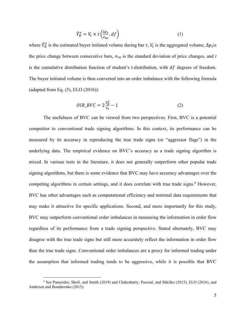
�� = �� × � �∆��∆ , �� (1)

where �� is the estimated buyer initiated volume during bar �, �� is the aggregated volume, ∆��is

the price change between consecutive bars, σ∆p is the standard deviation of price changes, and t

is the cumulative distribution function of student’s t-distribution, with �� degrees of freedom.

The buyer initiated volume is then converted into an order imbalance with the following formula

(adapted from Eq. (5), ELO (2016)):

��_�� = 2 �� − 1 (2)

The usefulness of BVC can be viewed from two perspectives. First, BVC is a potential

competitor to conventional trade signing algorithms. In this context, its performance can be

measured by its accuracy in reproducing the true trade signs (or “aggressor flags”) in the

underlying data. The empirical evidence on BVC’s accuracy as a trade signing algorithm is

mixed. In various tests in the literature, it does not generally outperform other popular trade

signing algorithms, but there is some evidence that BVC may have accuracy advantages over the

competing algorithms in certain settings, and it does correlate with true trade signs.6 However,

BVC has other advantages such as computational efficiency and minimal data requirements that

may make it attractive for specific applications. Second, and more importantly for this study,

BVC may outperform conventional order imbalances in measuring the information in order flow

regardless of its performance from a trade signing perspective. Stated alternately, BVC may

disagree with the true trade signs but still more accurately reflect the information in order flow

than the true trade signs. Conventional order imbalances are a proxy for informed trading under

the assumption that informed trading tends to be aggressive, while it is possible that BVC

6 See Panayides, Shofi, and Smith (2019) and Chakrabarty, Pascual, and Shkilko (2015), ELO (2016), and

Andersen and Bondarenko (2015).

6

actually measures informed trading whether it is aggressive or passive. We discuss the relevant

evidence for this potential property of BVC in Section 3 below.

BVC may be particularly advantageous in the context of markets where high frequency

trading is common. ELO (2016) assert that high speeds of trading, increased fragmentation, and

higher rates of order submissions and cancellations have changed the mechanics of trading in

ways that reduce the classification accuracy of conventional trade signing algorithms.7 ELO

(2016) also suggest that in the modern market environment the aggressor side of a trade is now

less likely to correlate with the informed side of the trade.

One potential drawback of BVC is that its output is not entirely deterministic. The

grouping of trades into bars can differ if the starting point changes. For example, consider two

researchers working on partially overlapping trade samples with different starting dates. If they

chose to fill bars continuously over the full sample (as in ELO (2016)), they would potentially

arrive at different bars for the overlapping trades. The situation is similar if two researchers use

the same sample but on chooses to fill bars continuously while the other restarts fresh with an

empty bar periodically (possibly every stock-month as in Panayides, Shofi, and Smith (2019) or

every trading day). Volatility estimation can also cause uncertainty in the output. σ∆p in Eq. (1) is

estimated in-sample using the full sample period in ELO (2016). Therefore, the volatility and

BVC classifications for a specific group of trades could differ depending on the starting or

ending dates of the samples they are included in. Further, if the researcher is concerned with

time-varying volatility, it would clearly be reasonable to re-estimate volatility over shorter

intervals. This would also potentially alter the output. Another related issue is that there is little

7 There is disagreement in the literature regarding this assertion. Chakrabarty, Pascual, and Shkilko (2015)

and Carrion and Kolay (2019) both report evidence that conventional trade signing algorithms perform well in data

from fast and fragmented markets, and Panayides, Shofi, and Smith (2019) report mixed evidence.

7

guidance in the literature on how to select the bar size for BVC. These problems could be

mitigated if researchers coordinated on a set of implementation details, but this has not happened

as of this writing. With the exception of some sensitivity analysis around bar size, these effects

have not been quantified in the literature so it is not clear if they are significant in practice.8

3. Existing Evidence on BVC and Informed Trading

First, we describe and discuss the evidence presented in ELO (2016). Next, we report the

results of a simulation exercise where we assess the statistical properties of the test specification

ELO (2016) by repeating their test in simulated data with no informed trading.

3.1 The ELO (2016) Test

The main evidence provided by ELO (2016) in support of the ability of BVC to identify

informed trading is provided by a regression designed to associate time variation in liquidity with

order flow imbalance measures.9 This is based on the idea that market makers will withdraw

liquidity when informed traders are active. The regression specification is:

��_� !"# = % + '(|��_��#| + '*|��_+��,#| + '-��_� !"#.( (3)

where CS_SPRD is the Corwin and Schultz (2012) high-low spread (Corwin-Schultz spread

hereafter), OIB_BVC is the order flow imbalance constructed using BVC, OIB_TICK is the

order flow imbalance constructed using the tick rule, and t indexes volume bars. The lagged

value of CS_SPRD is included as a control for autocorrelation, and t-statistics are Newey-West

adjusted.

8 See Chakrabarty, Pascual, and Shkilko (2015), Masot, Nawn, and Pascual (2018), and Panayides, Shofi,

and Smith (2019). 9 ELO (2016) also present related evidence graphically in their Figure 5, but without an accompanying

statistical test.

8

The results of this test are presented in Table 6 of ELO (2016). Three versions of the

regression model are estimated: one with OIB_BVC, one with OIB_TICK and a third with both.

All three versions include the lagged CS_SPRD. The coefficient on |OIB_BVC| is positive and

significant and the coefficient on |OIB_TICK| is negative and significant. These results are

consistent across models. ELO (2016) interpret these results as evidence that BVC works to

measure informed trading, and that the tick rule order imbalances identify aggressive traders that

tend to be uninformed. We discuss several observations and concerns with this test below.

First, we note that the main conclusion is only supported by the result of a single time

series regression, using a single test asset and a single BVC parameterization. The rationale for

this choice is not explained in the paper, and a separate analysis in ELO (2016) uses three test

assets and ten BVC parameterizations for each. Regardless of the rationale, it seems difficult to

draw strong conclusions from these results without evidence of robustness.

Second, this test relies on reductions in liquidity provision by market makers to detect

informed trading. In contrast to other tests in the literature that use permanent price impacts,

future returns, or other price-discovery based measures, this test relies on a near-immediate

market maker response to detect informed trading. As Kacperczyk and Pagnotta (2016) state,

“most theory-motivated information measures, such as the bid–ask spread and the price impact

of trades (Glosten and Milgrom, 1985; Kyle, 1985), rely on the notion that the presence of

informed traders is common knowledge to other market participants.” This is essentially a joint

hypothesis problem, where the test relies not only on the presence of informed trading but also

on the nature of the response by market makers. This immediate response is inconsistent with

some theories where market makers learn over a series of trades or informed traders attempt to

9

hide their informed status.10 If market makers respond slowly to informed imbalances, or

withdraw liquidity while patient liquidity demanders continue to post quotes at the old prices,

these tests will misclassify the imbalances as uninformed. We do not suggest that this issue

invalidates this test, as it is based on a theoretically sound response to informed trading. It seems

reasonable, however, to take the nature of this test into account when determining how much

weight to place on these results and as motivation to seek confirmation from other tests.

Third, it is not clear that the Corwin-Schultz spread is well-suited to this test. This test is

designed to associate time variation in liquidity provision with the time variation in informed

trading captured by the explanatory variables. The Corwin-Schultz spread relies only on trade

data, and ELO (2016) motivate their choice of this liquidity measure with concerns about the

reliability of quote data from fast markets. The Corwin-Schultz spread as originally introduced,

however, estimates an average spread over a series of observations and treats time variation

between adjacent observations as noise to be averaged out rather than as meaningful time

variation. In their monthly analysis, Corwin and Schultz (2012) discard all stock-months where

they are not able to average over at least 12 trading days. Corwin and Schultz (2012) also find

time variation in individual observations when using simulated data with a constant bid-ask

spread, including negative spread observations.11 Similarly, in our analysis below we find

significant time variation in the Corwin-Schultz spread, including negative observations, in

simulated data with a constant trading cost function.12 ELO (2016) use the individual spread

observations directly without smoothing or aggregation.

10 For example, in Kyle (1985) the informed trader trades slowly to blend in with liquidity traders, and its

private information is only revealed gradually in prices. 11 Corwin and Shultz (2012) investigate alternate adjustments for negative spreads and find that setting

negative spreads to 0 before averaging results in the best performance. 12 Not tabulated, available upon request.

10

Fourth, the BVC order imbalance is only competed against the tick rule order imbalance

and not the true order imbalance. One of the most important hypothesized properties of BVC is

its potential advantage over order imbalances constructed from true trade signs in identifying

informed trading.

Fifth, as others have pointed out in similar tests, there is a possibility that there is a

mechanical bias in regressions of this form.13 The Corwin-Schultz spread, used as the dependent

variable, is essentially a non-linear transformation of the high-low range in a bar. The BVC order

imbalance is essentially a non-linear transformation of the return in the bar, and the regressions

use the absolute value of this variable as an explanatory variable. The high-low range in a bar is

clearly mechanically related to the absolute value of the return in the bar, regardless of the

presence of informed trading.14 Therefore, one might expect regressions of the high-low range on

the contemporaneous absolute value of the return to be misspecified. It is not clear if the

transformations of the high-low range into the Corwin-Shultz spread and the absolute value of

the return into BVC break this mechanical relationship. While many of the other concerns we

raise in this section are qualitative and somewhat subjective, this issue is testable. We investigate

the properties of this regression specification in the next section.

3.2 Simulations

In this section, we conduct a simulation exercise to investigate the properties of the ELO

(2016) regression tests. We simply reproduce these regressions repeatedly in simulated data with

no informed trading. If these tests are well specified, the coefficients of interest will be zero on

13 See Chakrabarty, Pascual, and Shkilko (2015) and Andersen and Bondarenko (2015). 14 We are not aware of an analytical proof of this relationship, but it is easily demonstrated with

simulations.

11

average and their test statistics will reject the null hypothesis at an appropriate rate for the

specified significance level.

ELO (2016) only conduct their tests on BVC order imbalances constructed with 10,000

contract volume bars. However, they advance no arguments that this bar size is optimal and

provide no cautions that their results should be sensitive to bar size. They use bar sizes from

1,000 – 25,000 contracts in other sections of their paper. Therefore, we reproduce tests on order

imbalances constructed with 1,000, 10,000, and 25,000 contract bars. In each test, we follow

ELO (2016) in using the same bar size to calculate the Corwin-Shultz spread as that used to

calculate the BVC order imbalances.

To generate data with no informed trading, we use a version of the Glosten and Harris

(1988) model with the adverse selection component of the spread set to zero. Our

implementation of the model can be summarized as follows:

/# = /#.( +0# (4)

0#~2(0, 56) (5)

# = /# + 8#(9: + 9((�# − 1)) (6)

Where mt is the pre-trade midpoint (or, equivalently in this setting, the fair value of the security)

for trade t, Pt is the trade price for trade t, Qt is a trade sign indicator variable for trade t taking

the value of 1 for a buy trade and -1 for a sell trade, Vt is the unsigned volume of trade t, c0 and

c1 are trading cost parameters, and εt is the change in pre-trade midpoint due to public

information. We subtract one contract from Vt so c0 will match the half bid-ask spread exactly

for a one contract trade. Note that we simulate the model in event time rather than calendar time.

In this data generated from this model, trades have no permanent price impact at all.

12

For our main simulations, we generate signed trade volumes from a normal distribution,

round to the nearest contract, and use these signed volumes to calculate Qt and Vt. We also adjust

small trade sizes up to one contract before rounding to eliminate zero contract trades. This

procedure generates less skewness in trade size than that reported by ELO (2016), which we

believe is conservative in that it will likely lead to data with better-behaved statistical properties.

The price dynamics in these simulations contain no features resembling informed trading

and can be described simply as follows. Future midpoint price changes are uncorrelated with

trades. Trade prices only deviate from the pre-trade midpoints by temporary price impacts which

disappear by the next trade. These temporary price impacts include half the bid-ask spread plus a

linear function of the volume traded, which can be viewed as the effect of larger trades “walking

the book.” One could employ richer models that simulate other microstructure effects such as

autocorrelated order flow induced by order-splitting, inventory effects, time-varying volatility, or

imperfect resiliency where temporary price impacts decay slowly instead of disappearing by the

next trade. A well-specified test for informed trading should be robust to these effects, which

could generate patterns that share some features of informed trading and can be present in a

market with no informed trading. However, given the results for the simple simulation tests we

report below, we consider richer simulations unnecessary in this case.

For each bar size, we simulate 1,000 trials. For each trial we generate a dataset of

128,579,415 trades, matching the ELO (2016) ES sample. We choose our other simulation

parameters to approximately match the summary statistics reported by ELO (2016) for their

sample and other known characteristics of the ES market. Table 1 reports the simulation

parameters. Figure 1 shows the price path for a randomly selected trial. Next, in each trial we

form volume bars and calculate the BVC order imbalances and Corwin-Schultz spreads as

13

described above. In place of tick rule order imbalances, we calculate true order imbalances for

each bar using our simulation-generated trade signs. The true order imbalances are defined as:

��_+!;<# = �=>_�?@=ABC–EB@@_�?@=ABC�?@=ABC (7)

where BUY_VOLUMEt and SELL_VOLUMEt are the share volumes designated as buys and

sells in bar t and VOLUMEt is the total share volume in bar t.

Table 2 reports selected summary statistics from the simulated trades. In general, these

are similar to the ELO (2016) sample in the main dimensions. Of particular interest, the mean

Corwin-Schultz spread for the 10,000 contract bar size simulations is 22 bps, compared to 23 bps

in ELO (2016). The one notable difference is that the trade size distribution is less skewed than

the ELO (2016) sample as mentioned above; while the means are similar, the median in our

sample is 4 contracts compared to 1 contract in the ELO (2016) sample. While we attempt to

simulate data similar to that used in ELO (2016), we emphasize that this is for comparability

only; the validity of their regression model is not purported to be contingent on specific features

of the test asset or market, so we should not require a close match to their data in order to

investigate the regression specification properties of interest.

In each trial, we run variations of the following regression:

��_� !"# = % + '(|��_��#| + '*|��_+!;<#| + '-��_� !"#.( (8)

where all variables are as defined above. This regression is similar to Eq. (2), which corresponds

to Eq. (6) in ELO (2016). Aside from the inclusion of an intercept, our only deviation from Eq.

(2) is the replacement of the tick rule order imbalance with the true order imbalance. This choice

is motivated by the discussion in Section 3.1 above. We estimate three versions of the model that

vary only in the included imbalance variables: one version with only BVC order imbalance, one

14

with only the true order imbalance, and another with both. All versions include the lagged

Corwin-Shultz spread. We calculate Newey-West t-statistics.

Table 3 reports the average coefficients from Eq. (7) across all 1,000 trials for each bar

size/regression model combination, and t-statistics that test whether the average coefficient is

different from 0. Panel A reports results for 1,000 contract bars. Models 1 and 3 show that the

coefficient on |��_��#| is significantly positive, and Models 2 and 3 show that the average

coefficient on |��_+!;<#|is significantly negative. These results are qualitatively consistent

with the results reported in ELO (2016) for the 10,000 contract bar size, although the estimated

coefficients are smaller in magnitude. Panel B reports results for 10,000 contract bars. Models 1

and 3 show that the coefficient on |��_��#| is significantly negative, and Models 2 and 3

show that the average coefficient on |��_+!;<#|is insignificant. Panel C reports results for

25,000 contract bars. The results are similar to those for the 10,000 contract bars. Again Models

1 and 3 show that the coefficient on |��_��#| is significantly negative, and Models 2 and 3

show that the average coefficient on |��_+!;<#|is insignificant.

For all three parameterizations of BVC, these tests indicate a statistically significant

relationship between BVC and informed trading, despite being run on data with no informed

trading. Further, the relationship is not stable across BVC parameterizations. Taken literally,

when we divide the data into 1,000 contract bars, the tests indicate that BVC measures the

informed side of the order flow. However, for 10,000 and 25,000 contract bars, the tests indicate

that BVC measures the uninformed side. While these are clearly incorrect interpretations from

spurious results, it is noteworthy that the conclusions a researcher employing this test might form

are so sensitive to the BVC parameterization choices.

15

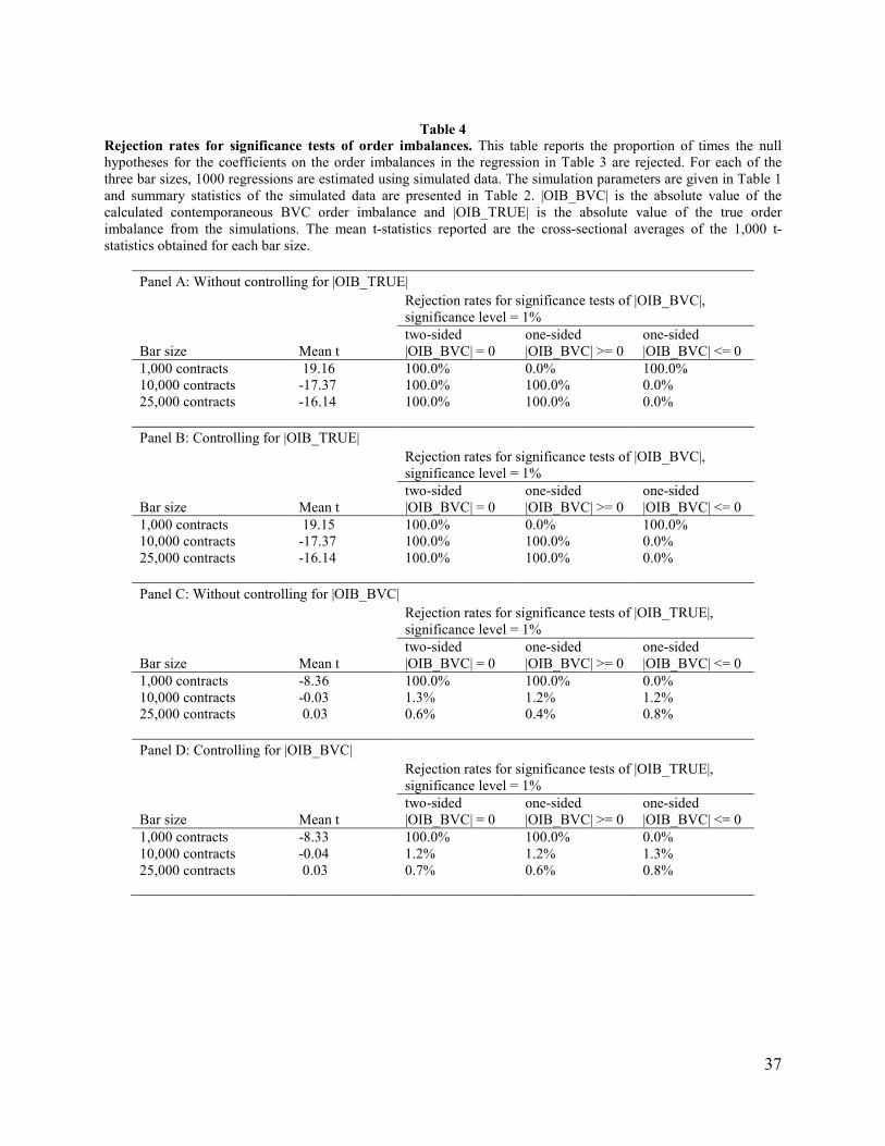
Table 4 provides an alternate perspective on these regressions. While Table 3 considers

results aggregated across all trials, Table 4 considers the distribution of Newey-West t-statistics

on the individual trials and reports associated rejection rates for the null hypotheses of no

relationship between the imbalance variables and informed trading. The data presented in Table

4 allows us to evaluate the size of the tests; given the lack of informed trading in the data, well-

specified tests should reject the null at approximately the specified significance level. Panels A

and B report rejection rates for hypothesis tests on the coefficient on |��_��#|. Panel A uses

tests from the regression model that omits |��_+!;<#| (corresponding to Model 1 in Table 3),

and Panel B uses tests from the regression model that controls for |��_+!;<#| (corresponding

to Model 3 in Table 3). Mean t-statistics are similar for both specifications and rejection rates are

identical. We use a 1% significance threshold.

The results in Table 4 Panels A and B are extreme. The two-sided test of the hypothesis

that the coefficient on |��_��#| is equal to zero is rejected for 100% of trials for all

parameterizations, with or without the |��_+!;<#| control. Every one of the 1,000 trials

incorrectly rejects the null in every specification tested. Similarly, the one-sided tests all reject

with at 100% or 0% rates. Recall that we are using a 1% significance level, so a well-specified

test would reject in approximately 1% of trials.15 In summary, in both models and for all three

bar sizes, we observe a Type 1 error in every single trial for the two-sided test and for one of the

one-sided tests. The asymmetry in the one-sided tests points to a bias, but the direction of the

bias changes with the parameterization of BVC and matches the direction suggested by the

aggregated results in Table 3.

15 Brown and Warner (1980) point out that, when the null is true and the test statistic is well-specified, the

rejection rate will not be exactly equal to the significance level; the rejection rate is a random variable with a

Bernoulli distribution. In our setting, this corresponds to a 95% confidence interval for rejection rates of (0.47% and

1.53%).

16

Table 4 Panels C and D report rejection rates for hypothesis tests on the coefficient on

|��_+!;<#|. Panel C uses tests from the regression model that omits |��_��#| (corresponding to Model 2 in Table 3), and Panel D uses tests from the regression model that

controls for |��_��#| (corresponding to Model 3 in Table 3). For 1,000 contract bars, the two-

sided tests reject 100% of the time in both models. Again, the one-sided tests reject the at 100%

or 0% rates in the directions suggested by the results in Table 3. For 10,000 and 25,000

contracts, however, the rejection rates in both models are much closer to the specified

significance level of 1%. For 10,000 contract bars, the rejection rates are all greater than 1% but

none are significantly different from 1% at the 5% level (i.e. all fall within the 95% confidence

interval around 1% given in Footnote 11). For 25,000 contract bars, the rejection rates are all

lower than 1%, but only significantly lower in one case (the 1-sided test of the null hypothesis of

|��_+!;<#| >= 0 without controlling for |��_��#|). The result that the rejection rates for

|��_+!;<#| are much more reasonable than those for |��_��#| for all but the small bar size

suggests that concerns of a mechanical relationship between |��_��#|and the Corwin-Shultz

spread have merit. However, the extreme misspecification observed for the 1,000 contract bars

indicates that this explanation is incomplete.

Note that for the 10,000 contract bar size the coefficient on |��_��#| is uniformly

significantly negative, while ELO (2016) uses this bar size and reports a significantly positive

coefficient. One might wonder whether this means the test is biased against the ELO (2016)

result and strengthens their conclusions. We do not believe that this is the correct interpretation.

First, given that the bias in this test is not stable across parameterizations, it is not likely to be

stable across characteristics of the data. As mentioned above, our simulated data omits many

features that may be present in real data such as order splitting, inventory effects, and imperfect

17

resiliency. Therefore, it would be an aggressive interpretation to claim that this negative result

holds uniformly in the absence of informed trading when bar sizes of 10,000 contracts or shares

are used to estimate BVC in actual market data. Second, it is important that the coefficients are

unbiased in this type of regression. In this specification, a negative coefficient has the specific

economic interpretation that BVC is measuring the trading of the uninformed counterparties of

informed order flow. It is therefore misleading to observe these negative coefficients when there

is no informed trading. Third, and perhaps most importantly, our results are so extreme that it is

difficult to rationalize using regressions of this form to measure the relationship between order

imbalances and informed trading. In our view, 100% rejection rates in these simulations indicate

a completely spurious regression rather than one containing a statistical issue that can be

overcome with an adjustment for a predictable bias or through inflation of the standard errors.

A reasonable question is whether the temporary price impacts in our simulations drive

our results by mimicking some dimension of informed trading. To investigate this possibility we

modify the simulations to omit the temporary price impacts and repeat the experiment.

Mechanically speaking, we set the c0 and c1 trading cost parameters in Eq. (6) to 0 and leave the

rest of the procedure unchanged. The midpoint prices then follow a random walk and all trades

take place at the midpoint, regardless of trade direction and size. The results are presented in

Tables A1 and A2 of Appendix A. Table A1 shows that the mean coefficients on |��_��#| are lower in magnitude than those in Table 3, but are all significantly negative. For the 1,000

contract bars this coefficient switches from the positive value shown in Table 3, and the signs

match for the larger bar sizes. The mean coefficients on |��_+!;<#| are close to zero and are

only significant for 1,000 contract bars. Table A2 reports extreme rejection rates for all

hypothesis tests involving |��_��#|. The lowest two-sided rejection rate is 38.7% for 25,000

18

contract bars. These rejection rates are generally lower than 100% rates observed in the

simulations that included temporary price impacts, but still indicate extreme misspecification.

Similarly, the one-sided tests either grossly over-reject or never reject. None of the rejection rates

for |��_+!;<#|are significantly different from 1%. This analysis shows that, while temporary

price impacts exacerbate the misspecification in the ELO (2016) test, the test is still grossly

misspecified when prices follow a random walk and are completely unrelated to trades.

Overall, we conclude that evidence in ELO (2016) in support of a relationship between

BVC and informed trading is unreliable. Our simulations show that the tests employed grossly

over-reject the null in the hypothesis test of central importance and are severely biased. Further,

the bias is unstable across BVC parameterizations and is not likely to be corrected with a simple

statistical adjustment.

4. Alternate Tests of the Relationship between BVC and Informed Trading

The evidence presented in Section 3 calls into question the previous evidence in the

literature supporting the relationship between BVC and informed trading. However, even if the

tests used in prior studies were flawed, BVC may still be a useful technique to measure informed

trading. In this section, we propose and implement what we believe to be improved tests to

assess this issue. We use the NASDAQ HFT dataset to conduct our tests, which we describe

below.

4.1 Motivation and Regression Specifications

We believe that the problems identified above with the tests conducted in ELO (2016)

primarily stem from timing issues. There is potentially a mechanical relationship between the

contemporaneous Corwin-Shultz spread and BVC order imbalance that mimics the hypothesized

19

informed trading effects. There are also theoretical arguments that this type of specification

could either miss information effects that occur with a delay if market makers recognize

informed order flow gradually or could confuse temporary price impacts with information

effects.

These issues can be avoided by employing tests that exploit the simple property that

informed trading will be in the direction of future returns. Informed buying (selling) will tend to

be followed by positive (negative) returns. We use tests that regress returns in intervals of

various lengths on signed order imbalances variables from the prior volume bar. We use

midpoint returns to mitigate the effects of bid-ask bounce. We interpret positive coefficients on

order imbalance variables as evidence that those variables are positively correlated with

informed trading. Related specifications have been used often in prior literature, see for example

Chordia and Subrahmanyam (2004), Kaniel and Liu (2006), and Kim and Stoll (2014).

We note a limitation to our tests. Information could be incorporated into prices too

rapidly after informed trades to be captured with this design. If prices do adjust almost

immediately after informed trades, then the information effects will be largely realized before the

end of the bar in which the trades occur. Other studies using similar designs address this issue by

combining contemporaneous and future price changes or returns into a single dependent variable

(Huang and Stoll (1996), Kaniel and Liu (2006), and others). Given that BVC uses

contemporaneous returns in its calculation, it is not obvious how a valid test can be designed that

include contemporaneous returns in the dependent variable. However, BVC cannot be calculated

until the end of a bar, so its relationship to information revealed after the bar is complete (which

our tests are designed to capture) is probably of greater interest. Regardless, we believe that

positive results in these tests could potentially provide reliable evidence of a relationship

20

between BVC and informed trading in the literature, while negative results would not rule out a

relationship between BVC and very short-lived information in our data.

We design our tests to address two questions. First, do BVC order imbalances improve on

the ability of true order imbalances to measure informed trading? And second, do BVC order

imbalances capture passive informed trading?

In our first set of tests, we simply compete the ability of BVC order imbalances against

true order imbalances to predict returns in post-bar intervals ranging from 15 seconds to 5

minutes.

!<+# = % + '*��_��#.( + '(��_+!;<#.( (9)

where RETt is the midpoint return computed in the interval from the first midpoint after the end

of the bar in which the order imbalance is measured until the first midpoint after the specified

time has elapsed, and other variables are as previously defined.

For our second set of tests, we construct a variable that is designed to isolate the

component of order flow attributable to passive informed trading if the claims ELO (2016) are

correct. We describe the construction of this variable as follows.

Trades in an interval (whether a volume, trade, or time bar) can be classified into the

categories VBB, VBS, VBN, VSS, VSB, and VSN, where V indicates the proportion of the interval’s

volume traded in that category, the first subscript denotes whether the aggressive side of the

trade bought or sold, and the second subscript denotes whether the more informed side of the

trade bought or sold. The second subscript is set to N when two uninformed traders trade with

each other. For example, VBS is the volume in the interval where aggressive uninformed buyers

trade with passive informed sellers.

21

A conventional order imbalance measure, using either true trade signs or a trade

classification algorithm, measures the buyer-initiated volume less the seller-initiated volume in a

block of trades. For a given block of trades, this measure can be represented as:

��_+!;< = (�� + ��E + ��G) − (�EE + �E� + �EG) (10)

Note that this measure does not require the researcher to identify the informed side of the trade,

only the aggressive side. We present this formula assuming true trade classifications are

observable, as when “aggressor flags” are provided. If trades are classified with error, this

relationship can be re-written with estimated variables and classification errors.

While OIB_TRUE mechanically measures the aggressive trading imbalance, it is often

used as a proxy for the informed trading imbalance. This is based on the assumption that

informed traders tend to trade more aggressively than uninformed traders. This assumption can

be stated as:

�� > �E� (11)

�EE > ��E (12)

BVC is used to construct a similar order imbalance variable. ELO (2016) argue that order

imbalances calculated using BVC capture information, and that when these order imbalances

differ from conventional order imbalances, the differences are due to information rather than

error. Therefore, if these claims are correct, we can represent a BVC order imbalance as:

��I = (�� + �E�) − (�EE + ��E) (13)

Note that this representation ignores classification errors; we do not mean to imply that ELO

(2016) claim that this classification is perfect.

22

Using this representation, we can see that the difference between a BVC order imbalance

and a conventional order imbalance should contain information. Taking this difference and

simplifying, we find:

��I − ��JK=B= L(�� + �E�) − (�EE + ��E)M − L(�� + ��E + ��G) − (�EE + �E� + �EG)M

= 2(�E� −��E) + (�EG − ��G) (14)

For brevity we refer to this difference variable as OIB_DIFF hereafter. The first term is twice the

imbalance between informed traders buying passively and those selling passively. The second

term is an imbalance between uninformed traders selling aggressively and those buying

aggressively. Therefore, the first term should positively predict future returns while the second

should have no effect, so the total difference term should positively predict future returns.16 With

perfect BVC classification, all passive informed trading in the bar should be isolated in this

difference variable and no aggressive informed trading should be included. If BVC classification

is noisy but on balance adequate, the sign of this variable should still tend to indicate the

direction of passive informed trading. This motivates the following regression specification for

our second set of tests:

!<+# = % + '(��_"�NN#.( (15)

For both tests, we estimate the regressions one stock at a time, and average the

coefficients from these time series regressions across stocks in a reverse Fama and MacBeth

(1973) procedure. For each coefficient, we calculate the t-statistic on the cross-sectional mean

and also calculate Newey-West t-statistics for each stock.

16 For now we are ignoring the reversals of temporary price impacts for simplicity. If material, this effect

should bias the test in favor of associating OIB_DIFF with informed trading.

23

4.2 Data

We conduct our tests in the NASDAQ HFT dataset, which contains trade and quote data

for a sample of 120 stocks over a subset of dates in 2008-2010. This dataset is also used in

Brogaard (2012), Carrion (2013), and Brogaard, Hendershott, and Riordan (2014), O’Hara, Yao,

and Ye (2014), Carrion and Kolay (2019), and others. The 120 stocks in this sample were chosen

with a stratified random sampling approach along the dimensions of market capitalization and

listing venue.17 Market capitalization is evenly split between small, medium and large firms.

Listing venues are split equally between NASDAQ and NYSE. We utilize two subsets of data

from this dataset: trade reports and the NASDAQ Inside Quotes (BBO). The trade sample covers

each trading date during 2008 and 2009 and the week of Feb 22 – 26, 2010. For each sample

stock and date, each trade executed on the NASDAQ exchange is shown, excluding trades done

in the opening, closing, and intraday crosses. Trades include a millisecond timestamp and are

signed to indicate whether they were initiated by a buyer or seller. The trade signs are based on

records of fee and rebate payments used by the exchange. The NASDAQ BBO data is available

only for the following subset of dates: 1) the first full week of the first month of each quarter

during 2008 and 2009; 2) the crisis week of Sept 15 – 19, 2008; and 3) the week of Feb 22 – 26,

2010. We apply a filter to the sample to remove trades and quotes occurring before 9:30 am and

after 4:00 pm.

There are several benefits of using this dataset for our analysis. First, it contains true

trade signs, which we use to create true order imbalances. Second, NASDAQ notes that trade and

quote sequencing is of high quality in this dataset, which is particularly relevant for our analysis.

17 Sample was chosen by Ryan Riordan and Terrence Hendershott. See Brogaard (2013) and Carrion (2013)

for further details.

24

Third, this data is drawn from a market characterized by pervasive high-frequency trader (HFT)

participation and short durations between trades and quotes, which is the type of environment

where ELO (2016) argue that BVC should have advantages over conventional techniques.

Carrion and Kolay (2019) study the same data and report that HFTs participate in 75.16% of the

sample trades, the median time elapsed between quotes is 0.024 seconds, and the median time

elapsed between trades is 0.001 seconds.

This dataset is described in more detail in Carrion (2013), Brogaard, Hendershott, and

Riordan (2014), and Carrion and Kolay (2019).

4.3 BVC Implementation Details

Implementing BVC requires the researcher to make a number of decisions. The most

obvious are the basic parameterization – the bar size and volatility estimation. It is also necessary

to decide how to handle the overnight trading period and trades that overflow bars. There is little

relevant guidance or precedent in the literature. ELO (2016) note that implementation in equity

markets involves addressing new issues that they did not face in their futures data. Chakrabarty,

Pascual and Shkilko (2015) and Panayides, Shohfi, and Smith (2019) are the only other studies

we are aware of that have implemented BVC in equity data, and we follow their procedures

where appropriate.

We design bar sizes to be roughly equivalent to the bar sizes use by ELO (2016). In their

ES sample they use a range of bar sizes from 1,000 contracts to 25,000 contracts, and focus on

10,000 contract bars for their main test. The number of contracts per bar itself has very little

economic meaning across instruments. Therefore, instead of directly using these numbers as

share volume per bar, we scale bar sizes for each stock that approximately match the bars per

25

hour pace of the three bar sizes in ELO (2016). Considering the trading hours and average daily

volume, the ELO (2016) 1,000, 25,000, and 25,000 contract bar sizes approximately correspond

to 100, 10, and 4 bars per hour on average.18 After adjusting for 6.5 hour equity trading day,

these sizes correspond to averages of 650, 65, and 26 bars per day. For each stock, we convert

these to “bars per day” rules which are then applied to find fixed numbers of shares per bar every

month using the average in-sample daily volume for each stock-month. For brevity we refer to

these sizes as small, medium, and large bars hereafter.

We drop stock-months for a specific bar size where this approach would give a bar size

of less than 500 shares. Very small bar sizes do not result in well-formed bars. With bar sizes

around a typical trade size, BVC would not result in much aggregation. With bar sizes smaller

than the typical trade size, BVC would actually result in disaggregation where most trades are

split over multiple bars, which is clearly contrary to the spirit of BVC. This filtering leaves us

with a sample of 56 usable stocks for small bars, 112 stocks for medium bars, and 117 stocks for

large bars.

It is also necessary to estimate volatility for each stock to compute the CDF in Eq (1).

ELO (2016) use the in-sample standard deviation of bar-to-bar price changes over the whole

sample. In our data we have a longer sample period and each stock’s volatility may vary

significantly, so we use in-sample standard deviations of bar-to-bar price changes within each

stock-month.

18 The ES market is open an average of 23.55 hours per day and the ELO (2016) one-year sample contained

128,579,415 trades with an average size of 4.5 contracts.

26

To handle the overnight period, we discard the partially filled bar at the end of each day

and start a fresh bar with the first trade of the next day. We also use the close-open within-bar

price change for the first bar of the day rather than using the closing bar from the previous day.

Chakrabarty, Pascual and Shkilko (2015) and Panayides, Shohfi, and Smith (2019) note a

problem with large trades that span multiple bars. There may be a valid price change to use in Eq

(1) for the first bar, but for subsequent bars the open and the close are the same price. With no

price change, BVC evenly splits the volume in these bars between buys and sells. We apply a

correction for this issue proposed by Chakrabarty, Pascual, and Shkilko (2015). When a bar is

filled solely by volume from a single trade, we assign the same buy/sell split calculated for the

last bar which contained volume from multiple trades. This assumes that the first bar in each

cluster of bars with volume from a single trade generally contains volume from previous trades

and the beginning of the large trade. At the end of the cluster, we treat the first bar with volume

from multiple trades normally. This issue is likely to be more severe when using small bar sizes,

and partially motivates our filtering criteria of a required minimum bar size of 500 shares

discussed above.

We only use the subperiod that includes NASDAQ BBO data for our main tests, but we

use the full sample period to construct BVC order imbalances. This is important because the

BVC estimation benefits from using the longer period of contiguous data to compute the

standard deviations of bar-to-bar price changes.

4.4 Results

Our first set of tests use the regression model in Eq. (9) to compare the predictive power

of OIB_BVC and OIB_TRUE for future returns. The results are reported in Table 5. Panel A

27

reports results for the small bar size, which corresponds to an average of 650 bars per day. The

regressions only use 56 of the stocks, because reasonably well-formed BVC bars could not be

calculated for the remaining stocks at this small of a bar size.19 Using returns measured at all

three post-bar horizons (15 seconds, 1 minute, and 5 minutes), the coefficients on both order

imbalance variables are positive, indicating that these variables positively predict future returns

and suggesting that they are both correlated with information in the order flow. The coefficient

on OIB_TRUE is larger than that on OIB_BVC in all three models. Based on the t-statistic that

tests whether the mean coefficient for all stocks is equal to 0, OIB_TRUE is significant at all

three horizons, while OIB_BVC is significant at 15 seconds and marginally significant at 1

minute. Inspecting the distributions of t-statistics from the 56 individual regressions reveals a

similar pattern. The coefficients on OIB_TRUE have higher mean t-statistics, are more often

individually significantly positive, and less often significantly negative than the coefficients on

OIB_BVC. However, the coefficients on OIB_BVC are more often significantly positive than

negative. The predictive power of both variables weakens as the return horizon lengthens, but

predictive power of OIB_TRUE weakens more slowly and retains statistical significance at 5

minutes. Overall, for the small bar size, OIB_TRUE outperforms OIB_BVC in predicting future

returns, but the coefficients on OIB_BVC have the correct sign and are statistically significant at

shorter horizons.

Table 5 Panels B and C report results for medium and large bars. After filtering, 112

(117) stocks are usable with medium (large) bars. For all three return horizons and both bar sizes,

the coefficients on OIB_TRUE are positive and significant based on t-tests of the mean. The

distributions of the individual t-statistics show some weakening of significance with large bars

19 The relevant filtering criteria is described in Section 4.3.

28

and longer return horizons, however. OIB_BVC has no significant marginal predictive power for

future returns at these bar sizes. The mean coefficients are negative in four of the six

specifications and are never significantly different from zero. The distribution of individual t-

statistics tells a similar story; the means are always below 0.25 and often negative, and the

frequencies of significantly positive individual coefficients are much lower than observed with

small bars and sometimes lower than the number of significantly negative coefficients in the

same test.

Our second set of tests assesses the predictive power of OIB_DIFF for future returns. If

BVC successfully measures passive informed trading, this variable should isolate this component

of the order flow and positively predict returns. The results are reported in Table 6. Panel A

reports results for small bars, Panel B reports results for medium bars, and Panel C reports results

for large bars. The results are consistent across all bar sizes and return horizons. The mean

coefficients on OIB_DIFF are uniformly negative and statistically significant. Turning to the

distributions of t-statistics from individual regressions, the means are uniformly negative and less

than -2.0 for all small bar regressions and the medium bar regression with the 15 second horizon.

Few coefficients are positive and significant (ranging from 0/56 with small bars and 15 second

and 1 minute horizons to 4/117 with large bars and 5 minute horizons), while many are negative

and significant (ranging from 16/117 with large bars and 5 minute horizons to 55/56 with small

bars and 15 second horizons). In short, we see no evidence that OIB_DIFF can positively predict

returns, which is inconsistent with the hypothesis that OIB_BVC captures passive informed

trading.

How should we interpret the often-strong negative relationship between OIB_DIFF and

future returns? Mechanically, order flow only enters into the OIB_DIFF variable when

29

OIB_BVC differs in its buy-sell classification from OIB_TRUE. Therefore, regardless of

whether the difference is related to information or not, it takes on positive values for aggressive

selling and negative values for aggressive buying on the disagreed upon order flow. If neither

OIB_BVC nor OIB_TRUE capture informed trading and the disagreements between them are

random, then we should expect OIB_DIFF to have no predictive power for future returns.

However, if BVC does not capture passive informed trading and the disagreements are random,

but aggressive trading tends to be more informed than passive trading, then we should expect

OIB_DIFF to have negative predictive power for future returns. Therefore, what we observe is

consistent with OIB_TRUE capturing informed trading and the disagreed upon order flow

consisting of more random misclassification than passive informed trading.

Considering the hypothesized properties of BVC, we consider OIB_TRUE the most

interesting benchmark of OIB_BVC’s ability to identify informed trading. However, researchers

often use data that do not contain true trade signs and must rely on trade signing algorithms such

as the Lee and Ready method to estimate order imbalances. Therefore, in a robustness test we

repeat the analysis presented in Table 5 using order imbalances constructed from Lee and Ready

trade signs (OIB_LR) in place of OIB_TRUE.20 We describe the procedure in Appendix B and

report the results in Appendix Table B1. The results are very similar to those in Table 5. The

coefficients on OIB_LR are positive in every specification and generally significant, while the

coefficients on OIB_BVC have mixed signs and are only positive and significant for small bars

with a 15 second return horizon.

20 We do not repeat the OIB_DIFF tests from Table 6 using Lee and Ready order imbalances. These tests

would lose their interpretation as tests of BVC’s ability to measure passive informed trading if OIB_DIFF was

constructed using trades signed with error instead of true trade signs. This can be illustrated by modifying Eq. (14)

to incorporate trade signing errors.

30

Overall, we find no evidence that OIB_BVC outperforms OIB_TRUE or OIB_LR in

measuring informed trading and no evidence that OIB_BVC captures passive informed trading.

From our first set of tests, OIB_BVC does have some positive predictive power for future returns

when controlling for OIB_TRUE for small bar sizes and short horizons, but even in these cases it

underperforms OIB_TRUE and cannot be calculated for many stocks if one requires reasonably

well-formed bars.

5. Conclusions

Our analysis calls into question the use of BVC to measure informed trading. We identify

several issues with the evidence used to support this relationship in prior literature. Most

importantly, we conduct a simulation exercise that reproduces the main test used in the literature

in data with no informed trading, and find that the results are similar to those previously thought

to show a relationship between BVC and informed trading. Our simulation exercise shows that

these tests are severely misspecified, are sensitive the BVC parameterization, and are consistent

with a mechanical relationship between BVC and the liquidity measure used as a dependent

variable. We conduct independent tests of this relationship in the NASDAQ HFT dataset using a

research design that we believe avoids these problems. We find that conventional order

imbalances constructed from both true trade signs and Lee and Ready (1991) trade signs

uniformly outperform BVC in predicting future returns across multiple combinations of BVC

parameterizations and return measurement horizons. Additional tests uniformly fail to show that

the disagreements between BVC and true trade signs are driven by informed passive trading as

suggested by ELO (2016).

31

We note that BVC has many degrees of freedom, with little guidance from the literature

on how to best parameterize it. BVC is also arguably non-deterministic; even with a fixed

parameterization the same group of trades could be classified differently depending on the length

of the sample they are included in. These issues make it difficult to make conclusive statements

about the properties of BVC. It is possible that BVC can be improved by some implementation

strategy that we are not aware of.

We focus on the relationship between BVC and informed trading only, and our results

should not be interpreted to imply that BVC does not have other useful applications. ELO (2016)

and other studies have established that BVC can be used as a trade signing algorithm, and

nothing in this paper cautions against this application when the goal is unrelated to the

information content of the trade. Prior research has shown that BVC does not generally

outperform other algorithms with regard to trade signing accuracy, but it has computational

advantages, does not require quote data, and may be more robust to data sequencing errors than

other methods.

32

References

Andersen, Torben G., and Oleg Bondarenko, 2014a, VPIN and the flash crash, Journal of

Financial Markets 17, 1–46.

Andersen, Torben G., and Oleg Bondarenko, 2014b, Reflecting on the VPIN dispute, Journal of

Financial Markets 17, 53–64.

Andersen, Torben G., and Oleg Bondarenko, 2015, Assessing measures of order flow toxicity

and early warning signals for market turbulence, Review of Finance 19, 1-54.

Baruch, Shmuel, Marios Panayides, and Kumar Venkataraman, 2017, Informed trading and price

discovery before corporate events, Journal of Financial Economics 125, 561–588.

Brogaard, Jonathan, 2012, Essays on high frequency trading, Northwestern University

dissertation.

Brogaard, Jonathan, Terrence Hendershott, Ryan Riordan, 2014, High frequency trading and

price discovery, Review of Financial Studies 27, 2267–2306.

Brown, Stephen J., and Jerold B. Warner, 1980, Measuring security price performance, Journal

of Financial Economics 8, 205–258.

Carrion, Allen, 2013, Very fast money: High-frequency trading on the NASDAQ, Journal of

Financial Markets, 16, 680–711.

Carrion, Allen, and Madhuparna Kolay, 2019, Trade signing in fast markets, Financial Review,

forthcoming.

Chakrabarty, Bidisha, Roberto Pascual Gascó, and Andriy Shkilko, 2015, Evaluating trade

classification algorithms: Bulk volume classification vs. the tick rule and the Lee-Ready

algorithm, Journal of Financial Markets 25, 52–79.

Chordia, Tarun, Richard Roll, and Avanidhar Subrahmanyam, 2002, Order imbalance, liquidity,

and market returns, Journal of Financial Economics 65, 111–130.

Chordia, Tarun, and Avanidhar Subrahmanyam, 2004, Order imbalance and individual stock

returns: theory and evidence, Journal of Financial Economics 72, 485–518.

Corwin, Shane, and Paul Schultz, 2012, A simple way to estimate bid-ask spreads from daily

high and low prices, Journal of Finance 67, 719–759.

Easley, David, Marcos M. López de Prado, and Maureen O’Hara, 2012, Flow toxicity and

liquidity in a high-frequency world, Review of Financial Studies 25, 1457–1493.

Easley, David, Marcos M. López de Prado, and Maureen O’Hara, 2016, Discerning information

from trade data, Journal of Financial Economics 120, 269–285.

33

Easley, David, Marcos M. López de Prado, and Maureen O’Hara, 2014, VPIN and the Flash

Crash: A rejoinder, Journal of Financial Markets 17, 47–52.

Harris, Lawrence, 1998, Optimal dynamic order submission strategies in some stylized trading

problems, Financial Markets, Institutions and Instruments 7, 1–76.

Huang, Roger D., and Hans R. Stoll, 1996, Dealer vs. auction markets: a paired comparison of

execution costs on NASDAQ and the NYSE, Journal of Financial Economics 41, 313–357.

Kaniel, Ron, and Hong Liu, 2006, So what orders do informed traders use? Journal of Business

79 1867–1913.

Kacperczyk, Marcin, and Emiliano Pagnotta, 2016, Chasing private information, working paper.

Kim, Sukwon Thomas, and Hans R. Stoll, 2014, Are trading imbalances indicative of private

information? Journal of Financial Markets, 20, 151–174.

Kyle, Albert S., 1985, Continuous auctions and insider trading, Econometrica 53, 1315-1336.

Lee, Charles M. C., and Mark J. Ready, 1991, Inferring trade direction from intraday data,

Journal of Finance 46, 733–746.

Massot, Magdalena, Samarpan Nawn and Roberto Pascual, 2018, Bulk volume classification

under the microscope: Estimating the net order flow, working paper.

O’Hara, Maureen, 2015, High frequency market microstructure, Journal of Financial Economics

116, 257–270.

O’Hara, Maureen, Chen Yao, and Mao Ye, 2014, What’s not there: Odd-lots and market data,

Journal of Finance 69, 2199–2236.

Panayides, Marios, Thomas Shohfi, and Jared Smith, 2019, Bulk volume classification and

information detection, Journal of Banking and Finance 103, 113-129.

34

Table 1

Summary of Simulation Parameters. Signed trade volumes are generated from a normal distribution and are used

to calculate the unsigned trade volume and the trade sign indicator as per Eqs. 4, 5 and 6 in Section 3. Trades are

aggregated into volume bars of 1,000, 10,000, or 25,000 contracts. The number of trades per trial is matched to the

number of trades in the ELO (2016) E-mini S&P futures sample while other simulation parameters are chosen to

approximately match either the ELO (2016) E-mini S&P 500 futures sample characteristics or the E-mini S&P

futures' market characteristics. The number of trades per trial is matched to that in ELO's sample while the starting

E-mini S&P 500 futures midpoint is the settlement price of E-mini S&P futures on the day prior to the start of ELO's

sample period. The midpoint volatility corresponds to the closing value of VIX on the day prior to the start of ELO's

sample period (18.26) scaled to a per-trade value. The signed volume volatility is calibrated to match ELO's mean

trade size after adjustments. The Glosten & Harris (GH) trading costs parameter c0 is half of E-mini S&P futures

tick size while c1 is calibrated to match the mean Corwin-Shultz spread in ELO's sample with 10,000 contract bar

size. The bar volatility for each of the three bars is the midpoint volatility scaled to bar size.

Simulation Parameter Value

Number of trials for each bar size

1,000

Number of trades/trial 128,579,415

Starting E-mini S&P 500 futures midpoint 1,222

Midpoint volatility (per trade) 0.02

Signed volume volatility (contracts/trade) 5.6

Glosten & Harris trading cost parameter c0 0.125

Glosten & Harris trading cost parameter c2 0.09

Bar volatility, 1k bar size 2.98



35

Table 2

Simulation summary statistics. Mean order imbalances and Corwin-Schultz spread calculated from volume bars in

each trial. The calculation of BVC order imbalances and Corwin-Schultz spreads is as described in Section 4.3. As

in ELO, the Corwin-Schultz spreads are reported as a proportion of the price of a contract and order imbalances are

the absolute value of the estimated order imbalance as a fraction of the total volume in a bar.

Statistics Value

Trade Size, mean

4.53

Trade Size, median 4

Bar size = 1,000 contracts

Mean number of bars 582,896.7

Mean Corwin-Schultz spread 0.0019

Mean |OIB_BVC| 0.111

Mean |OIB_TRUE| 0.066











36

Table 3

Regressions of Corwin-Schultz spreads on order imbalances in simulated trade data. This table reports the

results of variations of the following regression:

��_� !"# = % + '(|��_��#| + '*|��_+!;<#| + '-��_� !"#.(

in simulated trade data. The simulation parameters are given in Table 1 and summary statistics of the simulated data

are presented in Table 2. CS_SPRD is the Corwin-Schultz spread, OIB_BVC is the BVC order imbalance, and

OIB_TRUE is the order imbalance constructed from true trade signs. The regression is estimated separately for each

of 1,000 draws of the data. Reported coefficients are means over all trials, and t-statistics that test the null that the

mean coefficient is equal to 0.

Variable Model

Panel A: Bar size = 1,000 contracts 1 2 3

Intercept 0.0015 0.0015 0.0015

(287.79) (289.73) (288.37)

|OIB_BVC| 0.0001 0.0001

(253.42) (253.40)

|OIB_TRUE| -0.0001 -0.0001

(-198.08) (-197.72)

CS_SPRDt-1 0.1774 0.1775 0.1774

(70.37) (70.41) (70.38)

Panel B: Bar size = 10,000 contracts 1 2 3

Intercept 0.0022 0.0021 0.0022

(329.14) (329.78) (329.00)

|OIB_BVC| -0.0018 -0.0018

(252.1) (252.24)

|OIB_TRUE| -0.00001 -0.00001

(-1.13) (-1.27)

CS_SPRDt-1 0.0532 0.0532 0.0532

(43.46) (43.43) (43.46)

Panel C: Bar size = 25,000 contracts 1 2 3

Intercept 0.0024 0.0023 0.0024

(312.61) (314.68) (312.76)

|OIB_BVC| -0.0044 -0.0044

(-246.93) (-246.91)

|OIB_TRUE| 0.00002 0.00002

(0.92) (1.06)

CS_SPRDt-1 0.0319 0.0319 0.0319

(41.11) (41.21) (41.11)

37

Table 4

Rejection rates for significance tests of order imbalances. This table reports the proportion of times the null

hypotheses for the coefficients on the order imbalances in the regression in Table 3 are rejected. For each of the

three bar sizes, 1000 regressions are estimated using simulated data. The simulation parameters are given in Table 1

and summary statistics of the simulated data are presented in Table 2. |OIB_BVC| is the absolute value of the

calculated contemporaneous BVC order imbalance and |OIB_TRUE| is the absolute value of the true order

imbalance from the simulations. The mean t-statistics reported are the cross-sectional averages of the 1,000 t-

statistics obtained for each bar size.

Panel A: Without controlling for |OIB_TRUE|

Rejection rates for significance tests of |OIB_BVC|,

significance level = 1%

Bar size Mean t

two-sided

|OIB_BVC| = 0

one-sided

|OIB_BVC| >= 0

one-sided

|OIB_BVC| <= 0

1,000 contracts 19.16 100.0% 0.0% 100.0%

10,000 contracts -17.37 100.0% 100.0% 0.0%

25,000 contracts -16.14 100.0% 100.0% 0.0%

Panel B: Controlling for |OIB_TRUE|



Bar size Mean t

two-sided

|OIB_BVC| = 0

one-sided

|OIB_BVC| >= 0

one-sided

|OIB_BVC| <= 0

1,000 contracts 19.15 100.0% 0.0% 100.0%

10,000 contracts -17.37 100.0% 100.0% 0.0%

25,000 contracts -16.14 100.0% 100.0% 0.0%

Panel C: Without controlling for |OIB_BVC|

Rejection rates for significance tests of |OIB_TRUE|,


Bar size Mean t

two-sided

|OIB_BVC| = 0

one-sided

|OIB_BVC| >= 0

one-sided

|OIB_BVC| <= 0

1,000 contracts -8.36 100.0% 100.0% 0.0%

10,000 contracts -0.03 1.3% 1.2% 1.2%

25,000 contracts 0.03 0.6% 0.4% 0.8%

Panel D: Controlling for |OIB_BVC|



Bar size Mean t

two-sided

|OIB_BVC| = 0

one-sided

|OIB_BVC| >= 0

one-sided

|OIB_BVC| <= 0

1,000 contracts -8.33 100.0% 100.0% 0.0%

10,000 contracts -0.04 1.2% 1.2% 1.3%

25,000 contracts 0.03 0.7% 0.6% 0.8%

38

Table 5

Regressions of returns on order imbalances in equity trading data from the NASDAQ HFT dataset. This table

reports the results of the following regression:

!<+# = % + '*��_��#.( + '(��_+!;<#.(

for a sample of stocks selected for NASDAQ by Terrence Hendershott and Ryan Riordan. The full sample consists

of 61,271,087 trades for 120 stocks over the time periods January 2008 – December 2009 and February 22, 2010 –

February 26, 2010. !<+# is the midpoint-to-midpoint return from the end of the volume bar to a post-bar midpoint

after the return horizon has elapsed. ��JK=B,#.(is the lagged true order imbalance determined by rebate payments

from the data. ��_��#.( is the lagged order imbalance estimated using the BVC methodology as described in

Section 4.3. Panel A reports the result from 650 average bars per day, Panel B from 65 average bars per day and

Panel C 26 average bars per day. The number of stocks used drops below 120 in each panel since stocks which

cannot be distributed into well-formed bars get dropped from the sample. The coefficients and t-stats (raw and

Newey West corrected) reported are the averages across all stocks used in the regression. All coefficients are

multiplied by 1,000. Num pos sig (Num neg sig) represent the number of stocks for which the coefficient is positive

(negative) and significant.

Panel A: Average Bars per Day=650

N= 56 stocks

Variable Coefficient

t-statistic

Num

pos sig

Num

neg sig Return Horizon t(mean) mean(t )

15 seconds Intercept 0.0171 0.94 0.09 5 6

OIB_BVC 0.1104 2.71 2.59 34 3

OIB_TRUE 0.2518 6.62 9.90 56 0

1 minute Intercept 0.0406 1.21 0.27 4 1

OIB_BVC 0.1682 1.82 2.48 35 2

OIB_TRUE 0.2654 4.11 5.14 47 0

5 minutes Intercept 0.0498 1.1 0.07 3 2

OIB_BVC 0.0492 0.46 0.69 13 4

OIB_TRUE 0.2367 3.17 2.09 28 1

Panel B: Average Bars per Day=65

N= 112 stocks


t-statistic

Num

pos sig

Num


15 seconds Intercept 0.0234 0.99 -0.12 5 0

OIB_BVC -0.0374 -0.58 0.22 8 4

OIB_TRUE 0.3261 6.81 2.78 68 0


OIB_BVC -0.0564 -0.54 0.12 5 3

OIB_TRUE 0.4564 4.97 2.01 55 1


OIB_BVC -0.0698 -0.54 -0.13 8 11

OIB_TRUE 0.4554 4.41 1.14 34 2

39

Panel C: Average Bars per Day=26

N= 117 stocks


t-statistic

Num

pos sig

Num



OIB_BVC 0.0479 0.62 0.20 4 2

OIB_TRUE 0.3300 4.76 1.46 36 0

1 minute Intercept 0.0127 0.62 -0.09 2 3

OIB_BVC -0.0736 -0.65 0.02 4 4

OIB_TRUE 0.4628 3.76 1.09 30 0


OIB_BVC 0.1427 0.99 0.18 7 2

OIB_TRUE 0.4315 2.76 0.67 18 3

40

Table 6

Regressions of returns on BVC – True order imbalance disagreement variable in equity trading data from

the NASDAQ HFT dataset. This table reports the results of the following regression:

!<+# = % + '(��_"�NN#.(




after � seconds have elapsed. ��_"�NN#.(is the lagged difference between the order imbalance estimated using the

BVC methodology and the true order imbalance, as described in Section 4.3. Panel A reports the result from 650

average bars per day, Panel B from 65 average bars per day and Panel C 26 average bars per day. The number of

stocks used drops below 120 in each panel since stocks which cannot be distributed into well-formed bars get

dropped from the sample. The coefficients and t-stats (raw and Newey West corrected) reported are the averages

across all stocks used in the regression. All coefficients are multiplied by 1,000. Num pos sig (Num neg sig)

represent the number of stocks for which the coefficient is positive (negative) and significant.


N= 56 stocks


t-statistic

Num

pos sig

Num



OIB_DIFF -0.2653 -6.9 -10.64 0 55


OIB_DIFF -0.2821 -4.41 -5.65 0 46


OIB_DIFF -0.2494 -3.37 -2.29 1 29


N= 112 stocks


t-statistic

Num

pos sig

Num



OIB_DIFF -0.2989 -6.16 -2.43 0 61


OIB_DIFF -0.4360 -4.72 -1.87 2 52


OIB_DIFF -0.4718 -4.63 -1.22 2 37

41


N= 117 stocks


t-statistic

Num

pos sig

Num



OIB_DIFF -0.2671 -4.03 -1.10 1 31


OIB_DIFF -0.4220 -3.51 -0.95 1 27


OIB_DIFF -0.3903 -2.62 -0.60 4 16

42

Figure 1

Trade Price Path from Single Trial of Simulation Exercise

43

Appendix A: Simulations without Temporary Price Impacts

In this section we repeat the analysis reported in Table 3 and Table 4 in simulated data

with no temporary price impacts. We generate data with no informed trading and no temporary

price impacts using following model:

# = /# = /#.( +0# (A1)

0#~2(0, 56) (A2)

Where mt is the pre-trade midpoint (or, equivalently in this setting, the fair value of the security)

for trade t and Pt is the trade price for trade t. Note that we simulate the model in event time

rather than calendar time. In this data generated from this model, trades have no temporary or

permanent price impact. This is equivalent to the modified Glosten and Harris (1998) model

described in Section 3.2. with the trading cost parameters c0 and c1 set to 0. The rest of the

procedure is identical to that described in Section 3.2, and we continue to use the relevant

parameters given in Table 1.

44

Table A1

Regressions of Corwin-Schultz spreads on order imbalances in simulated trade data with no temporary price

impacts. This table reports the results of variations of the following regression:

��_� !"# = % + '(|��_��#| + '*|��_+!;<#| + '-��_� !"#.(

in simulated trade data. The simulation parameters are given in Table 1, with the exception of the trading cost

parameters c0 and c1 which are set to 0. CS_SPRD is the Corwin-Schultz spread, OIB_BVC is the BVC order

imbalance, and OIB_TRUE is the order imbalance constructed from true trade signs. The regression is estimated

separately for each of 1,000 draws of the data. Reported coefficients are means over all trials, and t-statistics that test

the null that the mean coefficient is equal to 0.

Variable Model

Panel A: Bar size = 1,000 contracts 1 2 3

Intercept 0.0001 0.0001 0.0001

(286.83) (286.91) (286.68)

|OIB_BVC| -0.0001 -0.0001

(-207.35) (-207.35)

|OIB_TRUE| -0.0000 -0.0000

(-4.47) (-4.73)

CS_SPRDt-1 0.0251 0.0251 0.0251

(158.3) (158.3) (158.3)

Panel B: Bar size = 10,000 contracts 1 2 3

Intercept 0.0003 0.0003 0.0003

(286.46) (284.96) (285.57)

|OIB_BVC| -0.0002 -0.0002

(-104.27) (-104.26)

|OIB_TRUE| 0.0000 0.0000

(0.2) (0.17)

CS_SPRDt-1 0.0174 0.0174 0.0174

(83.35) (83.36) (83.37)

Panel C: Bar size = 25,000 contracts 1 2 3

Intercept 0.0005 0.0005 0.0005

(285.28) (285.17) (284.14)

|OIB_BVC| -0.0004 -0.0004

(-70.24) (-70.22)

|OIB_TRUE| 0.0000 0.0000

(0.04) (0.05)

CS_SPRDt-1 0.0163 0.0163 0.0163

(58.6) (58.66) (58.61)

45

Table A2

Rejection rates for significance tests of order imbalances in simulated trade data with no temporary price

impacts. This table reports the proportion of times the null hypotheses for the coefficients on the order imbalances

in the regression in Table A1 are rejected. For each of the three bar sizes, 1000 regressions are estimated using

simulated data. The simulation parameters are given in Table 1, with the exception of the trading cost parameters c0

and c1, which are set to 0. |OIB_BVC| is the absolute value of the calculated contemporaneous BVC order imbalance

and |OIB_TRUE| is the absolute value of the true order imbalance from the simulations. The mean t-stats reported

are the cross-sectional averages of the 1,000 t-stats obtained for each bar size.

Panel A: Without controlling for |OIB_TRUE|



Bar size Mean t

two-sided

|OIB_BVC| = 0

one-sided

|OIB_BVC| >= 0

one-sided

|OIB_BVC| <= 0

1,000 contracts -10.04 100.0% 100.0% 0.0%

10,000 contracts -3.61 83.3% 89.9% 0.0%

25,000 contracts -2.29 38.7% 47.9% 0.0%

Panel B: Controlling for |OIB_TRUE|



Bar size Mean t

two-sided

|OIB_BVC| = 0

one-sided

|OIB_BVC| >= 0

one-sided

|OIB_BVC| <= 0

1,000 contracts -10.04 100.0% 100.0% 0.0%

10,000 contracts -3.61 83.2% 89.9% 0.0%

25,000 contracts -2.29 38.7% 48.1% 0.0%

Panel C: Without controlling for |OIB_BVC|



Bar size Mean t

two-sided

|OIB_BVC| = 0

one-sided

|OIB_BVC| >= 0

one-sided

|OIB_BVC| <= 0

1,000 contracts -0.14 1.2% 1.3% 1.1%

10,000 contracts 0.01 1.1% 1.2% 0.9%

25,000 contracts 0.00 1.1% 1.0% 0.7%

Panel D: Controlling for |OIB_BVC|



Bar size Mean t

two-sided

|OIB_BVC| = 0

one-sided

|OIB_BVC| >= 0

one-sided

|OIB_BVC| <= 0

1,000 contracts -0.15 1.2% 1.3% 1.1%

10,000 contracts 0.01 1.1% 1.2% 0.8%

25,000 contracts 0.00 1.1% 0.9% 0.7%

46

Appendix B: Regressions of Returns on BVC and Lee and Ready Order Imbalances

In this section we repeat the analysis reported in Table 5 using order imbalances

constructed from trades signed with the Lee and Ready method instead of true trade signs. We

first sign trades using the Lee and Ready method. The Lee and Ready method applies the quote

rule where possible and the tick rule otherwise. In our implementation of the quote rule, we

match trades with the most recent pre-trade quote midpoint that is not in the same millisecond as

the trade. Trades above the midpoint are classified as buys, and trades below the midpoint are

classified as sells. The tick rule is used when trade occurs at the midpoint of the matched quotes,

or in a small number of cases where no pre-trade quote is available. The tick rule compares the

current trade price with the preceding trade price and classifies the trade as a buy if the current

price is higher or a sell if the current price is lower. If the preceding trade price is identical to the

current price, the tick rule looks back to the most recent different price for a benchmark.

Next, we aggregate the signed trades in each bar into order imbalances as follows. The

true order imbalances are defined as:

��_O!# = �=>_�?@=ABC–EB@@_�?@=ABC�?@=ABC (B1)

where BUY_VOLUMEt and SELL_VOLUMEt are the share volumes designated as buys and

sells by the Lee and Ready method in bar t and VOLUMEt is the total share volume in bar t. The

bars are volume bars formed as described in Section 4.3.

For our regressions, we modify Eq. (9) as follows:

!<+# = % + '*��_��#.( + '(��_O!#.( (B2)

47

where OIB_LR is the Lee and Ready order imbalance defined in Eq. (B1) and other variables are

as previously defined. We estimate this regression one stock at a time and report the results in

Table B1 below.

48

Table B1

Regressions of returns on order imbalances in equity trading data from the NASDAQ HFT dataset. This table

reports the results of the following regression:

!<+# = % + '*��_��#.( + '(��_LR#.(




after the return horizon has elapsed. ��_O!#.(is the lagged order imbalance estimated using a modified Lee and

Ready (1991) algorithm that matches trades with the last quote in the prior millisecond. ��_��#.( is the lagged

order imbalance estimated using the BVC methodology as described in Section 4.3. Panel A reports the result from

650 average bars per day, Panel B from 65 average bars per day and Panel C 26 average bars per day. The number

of stocks used drops below 120 in each panel since stocks which cannot be distributed into well-formed bars get

dropped from the sample. The coefficients and t-stats (raw and Newey West corrected) reported are the averages

across all stocks used in the regression. All coefficients are multiplied by 1,000. Num pos sig (Num neg sig)

represent the number of stocks for which the coefficient is positive (negative) and significant.


N= 56 stocks


t-statistic

Num

pos sig

Num



OIB_BVC 0.0903 2.15 2.29 30 3

OIB_LR 0.2626 6.76 10.54 55 0


OIB_BVC 0.1294 1.36 2.17 28 2

OIB_LR 0.2901 4.37 5.80 48 0


OIB_BVC -0.0075 -0.07 0.43 11 3

OIB_LR 0.2751 3.53 2.60 30 0


N= 112 stocks


t-statistic

Num

pos sig

Num



OIB_BVC -0.0606 -0.84 0.15 5 4

OIB_LR 0.3638 7.19 3.00 71 0


OIB_BVC -0.0527 -0.52 0.04 5 4

OIB_LR 0.4699 5.25 2.29 62 0


OIB_BVC -0.1422 -1.02 -0.21 4 13

OIB_LR 0.5599 5.19 1.46 43 0

49


N= 117 stocks


t-statistic

Num

pos sig

Num



OIB_BVC 0.0156 0.22 0.14 2 2

OIB_LR 0.3781 5.45 1.66 49 0


OIB_BVC -0.0892 -0.71 -0.03 4 4

OIB_LR 0.5041 3.94 1.30 34 0


OIB_BVC 0.0959 0.35 0.13 6 3

OIB_LR 0.0505 3.51 0.87 24 4

Allen Carrion University of Memphis Madhuparna Kolay ...

Documents

Transcript of Allen Carrion University of Memphis Madhuparna Kolay ...